A nonlinear stochastic optimal bounded control using stochastic maximum principle

Abstract

A nonlinear stochastic optimal bounded control strategy for quasi-Hamiltonian systems with actuator saturation is proposed based on the stochastic averaging method and stochastic maximum principle. First, the averaged Itô stochastic differential equations are derived by using the stochastic averaging method for quasi-Hamiltonian systems. Then, the stochastic Hamiltonian system for optimal control with a given performance index is established based on the stochastic maximum principle. The bounded optimal control consisting of unbounded optimal control and bounded bang–bang control is determined by solving the forward-backward stochastic differential equations with control constraint. Finally, three examples of quasi-Hamiltonian systems with controls are given to illustrate the application of the proposed strategy. Numerical results show that the proposed control strategy significantly improves the control efficiency and chattering attenuation of the corresponding bang–bang control.

Keywords

Bounded control nonlinear stochastic optimal control stochastic averaging stochastic maximum principle stochastic quasi-Hamiltonian system

1. Introduction

Many structural systems in engineering can be modeled as a quasi-Hamiltonian system subjected to stochastic excitations. The nonlinear stochastic optimal control strategy (Zhu et al., 2001; Ying et al., 2003) for quasi-Hamiltonian systems with stochastic excitations has been proposed based on the stochastic averaging method (Zhu and Yang, 1997; Zhu et al., 1997) and stochastic dynamical programming principle (Stengel, 1986). At the same time, the optimal bounded control of dynamic systems under Gaussian white noise excitations has been studied and a hybrid solution to the dynamical programming equation was presented (Bratus et al., 2000; Dimentberg et al., 2000). The cell mapping method has been applied to solving the dynamical programming equation (Crespo and Sun, 2002). However, it is difficult to solve the partial differential dynamical programming equation of multi degree-of-freedom nonlinear systems.

On the other hand, the stochastic maximum principle can be used for designing a nonlinear stochastic optimal control, on which the study is relatively deficient. The maximum principle has some advantages (Kovaleva, 1999) and is particularly suitable for problems involving the active control of structural elements for vibration suppression (Sadek et al., 1996; Sloss et al., 2005). Based on the stochastic maximum principle, the stochastic optimal control problem is constructed in ordinary differential equations (Yong and Zhou, 1999). Several methods have been proposed for solving these equations, for example, the four step scheme. However, the stochastic optimal control for quasi-Hamiltonian systems with stochastic excitations based on the stochastic maximum principle needs to be studied further.

In fact, the control produced by an actuator is bounded due to the saturation and cannot achieve the strong stochastic control required. Several bounded control strategies have been proposed for eliminating or attenuating the chattering, including the sliding mode control (Bartolini and Punta, 2000; Bartoszewicz, 2000; Parra-Vega and Hirzinger, 2001) and the stochastic optimal bounded control for quasi-Hamiltonian systems based on the stochastic dynamical programming principle (Ying and Zhu, 2006; Feng, et al., 2012).

In the present paper, a new stochastic optimal bounded control strategy based on the stochastic averaging method and stochastic maximum principle is proposed for quasi-Hamiltonian systems with actuator saturation. The Itô stochastic differential equations are derived by using the stochastic averaging method for quasi-Hamiltonian systems. The stochastic Hamiltonian system for optimal control with a given performance index is established based on the stochastic maximum principle. The forward-backward stochastic differential equations with control constraints are solved for the adjoint process as a function of system energy. The optimal bounded control obtained consists of optimal unbounded control and optimal bang–bang control. Finally, the proposed strategy is applied to the controlled single degree-of-freedom nonlinear system, nonlinearly coupled Duffing oscillators and nonlinear cable structure subjected to Gaussian white noise excitations, and compared with the bang–bang control strategy.

2. Stochastic averaging of quasi-Hamiltonian systems

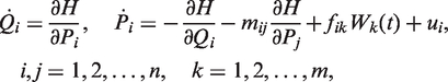
Consider the following controlled, stochastically excited and dissipated Hamiltonian system

{\overset{\cdot}{Q}}_{i} = \frac{\partial H}{\partial P_{i}}, {\overset{\cdot}{P}}_{i} = - \frac{\partial H}{\partial Q_{i}} - m_{ij} \frac{\partial H}{\partial P_{j}} + f_{ik} W_{k} (t) + u_{i}, i, j = 1, 2, \dots, n, k = 1, 2, \dots, m,

(1)

where Q_i and P_i are the generalized displacements and momenta, respectively;

Q = [Q_{1}, Q_{2}, \dots, Q_{n}] T

P = [P_{1}, P_{2}, \dots, P_{n}] T

;

H = H (Q, P)

is the Hamiltonian generally representing total system energy;

m_{ij} = m_{ij} (Q, P)

represent the coefficients of weak linear and/or nonlinear damping;

u_{i} = u_{i} (Q, P)

are the weak feedback control forces with bounds

| u_{i} | \leq b_{i}

due to actuator saturation;

u = [u_{1}, u_{2}, \dots, u_{n}] T

;

f_{ik}

denote the amplitudes of weak stochastic excitations;

W_{k} (t)

are the Gaussian white noises with correlation functions

E [W_{k} (t) \times W_{l} (t + τ)] = 2 D_{kl} δ (τ)

. There is

σ σ T = 2 fDf T

, where σ, f and D have elements

σ_{ik}

f_{ik}

and D_kl, respectively. The system (1) with m_ij = 0, f_ik = 0 and u_i = 0 is called a Hamiltonian system. The Hamiltonian system with n degrees-of-freedoms is completely integrable if there exist n independent integrals of motion in involution. The Hamiltonian system with n degrees-of-freedoms is completely non-integrable if there exists no independent integral of motion other than the Hamiltonian H. If the damping, stochastic excitations and controls are small compared with the total energy, i.e.,

m_{ij} = O (ɛ)

f_{ik} = O (ɛ 1 / 2)

and

u_{i} = O (ɛ)

, where ɛ is a small parameter, then the system (1) is called a quasi-Hamiltonian system.

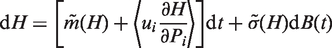
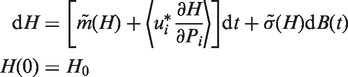
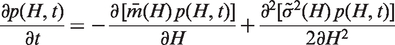
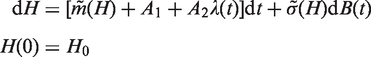
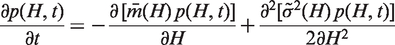
In the case of quasi-non-integrable Hamiltonian system, the Hamiltonian H is the only slowly varying process in system (1) while the other response quantities are rapidly varying processes. Since the slowly varying process is essential for describing the long-term behavior of the system, the stochastic averaging method for quasi-non-integrable Hamiltonian systems (Zhu and Yang, 1997) is used to average out the rapidly varying processes and to yield the following averaged Itô equation for the slowly varying process H (Zhu et al., 2001)

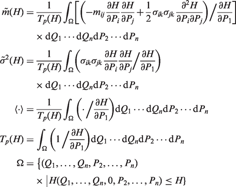
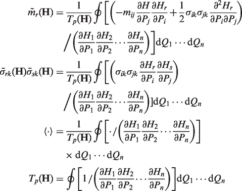
d H = [\tilde{m} (H) + á u_{i} \frac{\partial H}{\partial P_{i}} ñ] d t + \tilde{σ} (H) d B (t)

(2)

where B(t) is a unit Wiener process; the averaged drift and diffusion coefficients are

\tilde{m} (H) = \frac{1}{T_{p} (H)} \int_{Ω} [(- m_{ij} \frac{\partial H}{\partial P_{i}} \frac{\partial H}{\partial P_{j}} + \frac{1}{2} σ_{ik} σ_{jk} \frac{\partial 2 H}{\partial P_{i} \partial P_{j}}) / \frac{\partial H}{\partial P_{1}}] \times d Q_{1} \dots d Q_{n} d P_{2} \dots d P_{n} \tilde{σ} 2 (H) = \frac{1}{T_{p} (H)} \int_{Ω} (σ_{ik} σ_{jk} \frac{\partial H}{\partial P_{i}} \frac{\partial H}{\partial P_{j}} / \frac{\partial H}{\partial P_{1}}) \times d Q_{1} \dots d Q_{n} d P_{2} \dots d P_{n} 〈 \cdot 〉 = \frac{1}{T_{p} (H)} \int_{Ω} (\cdot / \frac{\partial H}{\partial P_{1}}) d Q_{1} \dots d Q_{n} d P_{2} \dots d P_{n} T_{p} (H) = \int_{Ω} (1 / \frac{\partial H}{\partial P_{1}}) d Q_{1} \dots d Q_{n} d P_{2} \dots d P_{n} Ω = {(Q_{1}, \dots, Q_{n}, P_{2}, \dots, P_{n}) \times | H (Q_{1}, \dots, Q_{n}, 0, P_{2}, \dots, P_{n}) \leq H}

(3)

Note that the dimension of the control system is reduced from 2n to 1 and the system state control is converted into the system energy control. The averaging operation of the second term on the right-hand side of equation (2) will be completed when u_i are determined.

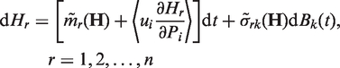
In the case of quasi-integrable Hamiltonian system (1), the stochastic averaging method for quasi-integrable Hamiltonian systems (Zhu et al., 1997) can be used to yield the averaged Itô equations. The equations for integrable and non-resonant case are

d H_{r} = [{\tilde{m}}_{r} (H) + á u_{i} \frac{\partial H_{r}}{\partial P_{i}} ñ] d t + {\tilde{σ}}_{rk} (H) d B_{k} (t), r = 1, 2, \dots, n

(4)

where

H = [H_{1}, H_{2}, \dots, H_{n}] T

; H_r are the averaged independent integrals of motion; B_k(t) are independent unit Wiener processes; the averaged drift and diffusion coefficients are

{\tilde{m}}_{r} (H) = \frac{1}{T_{p} (H)} \oint [(- m_{ij} \frac{\partial H}{\partial P_{j}} \frac{\partial H_{r}}{\partial P_{i}} + \frac{1}{2} σ_{ik} σ_{jk} \frac{\partial 2 H_{r}}{\partial P_{i} \partial P_{j}}) / (\frac{\partial H_{1}}{\partial P_{1}} \frac{\partial H_{2}}{\partial P_{2}} \dots \frac{\partial H_{n}}{\partial P_{n}})] d Q_{1} \dots d Q_{n} {\tilde{σ}}_{rk} (H) {\tilde{σ}}_{sk} (H) = \frac{1}{T_{p} (H)} \oint [(σ_{ik} σ_{jk} \frac{\partial H_{r}}{\partial P_{i}} \frac{\partial H_{s}}{\partial P_{j}}) / (\frac{\partial H_{1}}{\partial P_{1}} \frac{\partial H_{2}}{\partial P_{2}} \dots \frac{\partial H_{n}}{\partial P_{n}})] d Q_{1} \dots d Q_{n} 〈 \cdot 〉 = \frac{1}{T_{p} (H)} \oint [\cdot / (\frac{\partial H_{1}}{\partial P_{1}} \frac{\partial H_{2}}{\partial P_{2}} \dots \frac{\partial H_{n}}{\partial P_{n}})] \times d Q_{1} \dots d Q_{n} T_{p} (H) = \oint [1 / (\frac{\partial H_{1}}{\partial P_{1}} \frac{\partial H_{2}}{\partial P_{2}} \dots \frac{\partial H_{n}}{\partial P_{n}})] d Q_{1} \dots d Q_{n}

(5)

3. Bounded optimal control using stochastic maximum principle

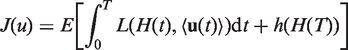
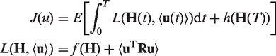
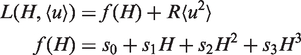
Assume that the performance index associated with control system (2) is (Zhu et al., 2001)

J (u) = E [\int_{0}^{T} L (H (t), 〈 u (t) 〉) d t + h (H (T))]

(6)

where

E [\cdot]

is the expecting operator; L(H, 〈u〉) is a cost function; h(H(T)) represents the final cost; T is the terminal time. The cost function is quadratic in control, i.e.,

L (H, 〈 u 〉) = f (H) + 〈 u T Ru 〉

(7)

where R is a positive-definite symmetric matrix assumed as diagonal and

f (H) > 0

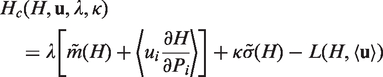
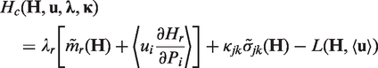
According to the stochastic maximum principle (Yong and Zhou, 1999), the stochastic optimal control of system (2) with performance index (6) is converted into a stochastic Hamiltonian system consisting of stochastic differential equations and a maximum condition for Hamiltonian. The associated Hamiltonian function H_c of the control system is

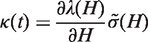
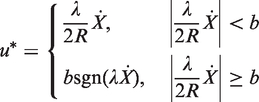
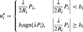
H_{c} (H, u, λ, κ) = λ [\tilde{m} (H) + á u_{i} \frac{\partial H}{\partial P_{i}} ñ] + κ \tilde{σ} (H) - L (H, 〈 u 〉)

(8)

where λ and κ are adjoint processes. For the bounded control with symmetric bound b_i > 0, the constraint domain U is

| u_{i} | \leq b_{i}

. By using the maximum condition

H_{c} (H, u *, λ, κ) = {max}_{u \in U} H_{c} (H, u, λ, κ)

(9)

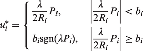
and noting that the Hamiltonian is concave with respect to u, the bounded optimal control obtained is then

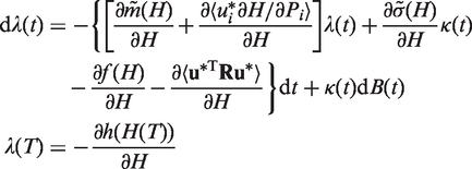
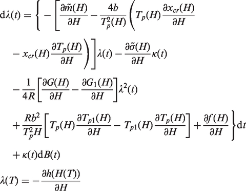
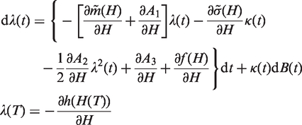
u_{i}^{*} = {\frac{λ}{2 R_{i}} P_{i}, | \frac{λ}{2 R_{i}} P_{i} | < b_{i} b_{i} sgn (λ P_{i}), | \frac{λ}{2 R_{i}} P_{i} | \geq b_{i}

(10)

The corresponding first-order adjoint equation is

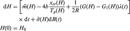
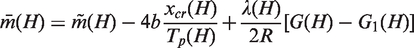
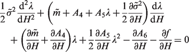
d λ (t) = - {[\frac{\partial \tilde{m} (H)}{\partial H} + \frac{\partial 〈 u_{i}^{*} \partial H / \partial P_{i} 〉}{\partial H}] λ (t) + \frac{\partial \tilde{σ} (H)}{\partial H} κ (t) - \frac{\partial f (H)}{\partial H} - \frac{\partial 〈 u * T Ru * 〉}{\partial H}} d t + κ (t) d B (t) λ (T) = - \frac{\partial h (H (T))}{\partial H}

(11)

Substituting the optimal bounded control (10) into equation (2), the following averaged Itô equation can be obtained

d H = [\tilde{m} (H) + á u_{i}^{*} \frac{\partial H}{\partial P_{i}} ñ] d t + \tilde{σ} (H) d B (t) H (0) = H_{0}

(12)

Equations (11) and (12) constitute the so-called forward-backward stochastic differential equations. They can be solved to obtain the adjoint process and the response of the controlled system. Note that equations (11) and (12) are ordinary differential equations different from the partial differential equation obtained by using the stochastic dynamical programming principle. An innovative solution procedure can be proposed for the optimal bounded control.

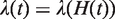
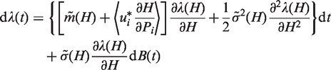
Suppose that the adjoint process λ(t) depends on time t only via system energy H(t), i.e.,

λ (t) = λ (H (t))

(13)

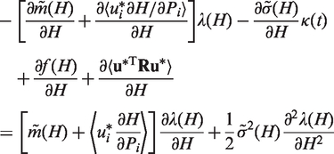
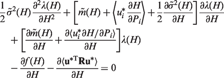
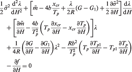
where λ(H) is a deterministic function. By differentiating equation (13) according to the Itô differential rule and using equation (12), the following expression is obtained

d λ (t) = {[\tilde{m} (H) + á u_{i}^{*} \frac{\partial H}{\partial P_{i}} ñ] \frac{\partial λ (H)}{\partial H} + \frac{1}{2} \tilde{σ} 2 (H) \frac{\partial 2 λ (H)}{\partial H 2}} d t + \tilde{σ} (H) \frac{\partial λ (H)}{\partial H} d B (t)

(14)

Comparing equation (14) with equation (11) leads to

- [\frac{\partial \tilde{m} (H)}{\partial H} + \frac{\partial 〈 u_{i}^{*} \partial H / \partial P_{i} 〉}{\partial H}] λ (H) - \frac{\partial \tilde{σ} (H)}{\partial H} κ (t) + \frac{\partial f (H)}{\partial H} + \frac{\partial 〈 u * T Ru * 〉}{\partial H} = [\tilde{m} (H) + á u_{i}^{*} \frac{\partial H}{\partial P_{i}} ñ] \frac{\partial λ (H)}{\partial H} + \frac{1}{2} \tilde{σ} 2 (H) \frac{\partial 2 λ (H)}{\partial H 2}

(15a)

κ (t) = \frac{\partial λ (H)}{\partial H} \tilde{σ} (H)

(15b)

Substituting equation (15b) into equation (15a) yields

\frac{1}{2} \tilde{σ} 2 (H) \frac{\partial 2 λ (H)}{\partial H 2} + [\tilde{m} (H) + á u_{i}^{*} \frac{\partial H}{\partial P_{i}} ñ + \frac{1}{2} \frac{\partial \tilde{σ} 2 (H)}{\partial H}] \frac{\partial λ (H)}{\partial H} + [\frac{\partial \tilde{m} (H)}{\partial H} + \frac{\partial 〈 u_{i}^{*} \partial H / \partial P_{i} 〉}{\partial H}] λ (H) - \frac{\partial f (H)}{\partial H} - \frac{\partial 〈 u * T Ru * 〉}{\partial H} = 0

(16)

Equation (16) is a deterministic ordinary differential equation. The deterministic function $λ (H)$ can be obtained by solving this equation, for example, using the finite difference algorithm for the finite time control with given terminal conditions. For the infinite time control with free terminal, the deterministic equation can be solved by using the iterative algorithm such as the Runge-Kutta algorithm with initial conditions corresponding to certain final values (Ying, et al., 2012). The deterministic function is used for calculating the bounded optimal control (10).

For the control system (4), the performance index is

J (u) = E [\int_{0}^{T} L (H (t), 〈 u (t) 〉) d t + h (H (T))] L (H, 〈 u 〉) = f (H) + 〈 u T R u 〉

(17)

where R is a positive-definite symmetric matrix assumed as diagonal and

f (H) > 0

. The Hamiltonian function of the control system with the separable Hamiltonian is

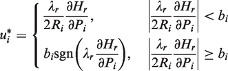
H_{c} (H, u, λ, κ) = λ_{r} [{\tilde{m}}_{r} (H) + á u_{i} \frac{\partial H_{r}}{\partial P_{i}} ñ] + κ_{jk} {\tilde{σ}}_{jk} (H) - L (H, 〈 u 〉)

(18)

where λ_r and κ_jk are adjoint process components. The bounded optimal control is obtained by using the maximum condition as

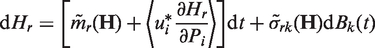
u_{i}^{*} = {\frac{λ_{r}}{2 R_{i}} \frac{\partial H_{r}}{\partial P_{i}}, | \frac{λ_{r}}{2 R_{i}} \frac{\partial H_{r}}{\partial P_{i}} | < b_{i} b_{i} sgn (λ_{r} \frac{\partial H_{r}}{\partial P_{i}}), | \frac{λ_{r}}{2 R_{i}} \frac{\partial H_{r}}{\partial P_{i}} | \geq b_{i}

(19)

The corresponding first-order adjoint equations and averaged system equations are

d λ_{r} (t) = - {[\frac{\partial {\tilde{m}}_{j} (H)}{\partial H_{r}} + \frac{\partial 〈 u_{i}^{*} \partial H_{j} / \partial P_{i} 〉}{\partial H_{r}}] λ_{j} (t) + \frac{\partial {\tilde{σ}}_{jk} (H)}{\partial H_{r}} κ_{jk} (t) - \frac{\partial f (H)}{\partial H_{r}} - \frac{\partial 〈 u * T Ru * 〉}{\partial H_{r}}} d t + κ_{rk} (t) d B_{k} (t)

(20)

d H_{r} = [{\tilde{m}}_{r} (H) + á u_{i}^{*} \frac{\partial H_{r}}{\partial P_{i}} ñ] d t + {\tilde{σ}}_{rk} (H) d B_{k} (t)

(21)

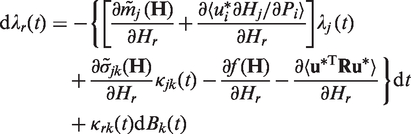
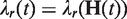
Suppose that the adjoint processes depend on time only via the integrals of motion

λ_{r} (t) = λ_{r} (H (t))

(22)

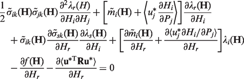
Differentiating equation (22) according to the Itô differential rule and comparing the equations with equation (20) yield the ordinary differential equations for adjoint processes

\frac{1}{2} {\tilde{σ}}_{ik} (H) {\tilde{σ}}_{jk} (H) \frac{\partial 2 λ_{r} (H)}{\partial H_{i} \partial H_{j}} + [{\tilde{m}}_{i} (H) + á u_{j}^{*} \frac{\partial H_{i}}{\partial P_{j}} ñ] \frac{\partial λ_{r} (H)}{\partial H_{i}} + {\tilde{σ}}_{ik} (H) \frac{\partial {\tilde{σ}}_{sk} (H)}{\partial H_{r}} \frac{\partial λ_{s} (H)}{\partial H_{i}} + [\frac{\partial {\tilde{m}}_{i} (H)}{\partial H_{r}} + \frac{\partial 〈 u_{j}^{*} \partial H_{i} / \partial P_{j} 〉}{\partial H_{r}}] λ_{i} (H) - \frac{\partial f (H)}{\partial H_{r}} - \frac{\partial 〈 u * T Ru * 〉}{\partial H_{r}} = 0

(23)

4. Examples

4.1. Nonlinearly single degree-of-freedom control system

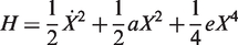
To illustrate the application and effectiveness of the proposed stochastic optimal bounded control strategy to a quasi-integrable Hamiltonian system, consider firstly the following nonlinear single degree-of-freedom control system

\overset{··}{X} + c \overset{\cdot}{X} + aX + eX 3 = W (t) + u

(24)

where X is a displacement; a and e are stiffness coefficients; c is a damping coefficient; W(t) is the Gaussian white noise with intensity 2D; u is a feedback control force. The associated Hamiltonian is

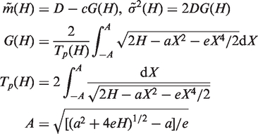
H = \frac{1}{2} \overset{\cdot}{X} 2 + \frac{1}{2} aX 2 + \frac{1}{4} eX 4

(25)

By applying the stochastic averaging method for quasi-integrable Hamiltonian systems, the averaged Itô stochastic differential equation is obtained as

d H = [\tilde{m} (H) + 〈 u \overset{\cdot}{X} 〉] d t + \tilde{σ} (H) d B (t)

(26)

where coefficients

\tilde{m} (H) = D - cG (H), \tilde{σ} 2 (H) = 2 DG (H) G (H) = \frac{2}{T_{p} (H)} \int_{- A}^{A} \sqrt{2 H - aX 2 - eX 4 / 2} d X T_{p} (H) = 2 \int_{- A}^{A} \frac{d X}{\sqrt{2 H - aX 2 - eX 4 / 2}} A = \sqrt{[(a 2 + 4 eH) 1 / 2 - a] / e}

(27)

The cost function in the performance index (17) is

L (H, 〈 u 〉) = f (H) + R 〈 u 2 〉 f (H) = s_{0} + s_{1} H + s_{2} H 2 + s_{3} H 3

(28)

According to the stochastic maximum principle, the optimal bounded control force is obtained as

u * = {\frac{λ}{2 R} \overset{\cdot}{X}, | \frac{λ}{2 R} \overset{\cdot}{X} | < b b sgn (λ \overset{\cdot}{X}), | \frac{λ}{2 R} \overset{\cdot}{X} | \geq b

(29)

where b is the control force bound. Substituting the control force (29) into equations (26) and (20) yields the following forward-backward stochastic differential equations

d H = [\tilde{m} (H) - 4 b \frac{x_{cr} (H)}{T_{p} (H)} + \frac{1}{2 R} (G (H) - G_{1} (H)) λ (t)] \times d t + \tilde{σ} (H) d B (t) H (0) = H_{0}

(30)

d λ (t) = {- [\frac{\partial \tilde{m} (H)}{\partial H} - \frac{4 b}{T_{p}^{2} (H)} (T_{p} (H) \frac{\partial x_{cr} (H)}{\partial H} - x_{cr} (H) \frac{\partial T_{p} (H)}{\partial H})] λ (t) - \frac{\partial \tilde{σ} (H)}{\partial H} κ (t) - \frac{1}{4 R} [\frac{\partial G (H)}{\partial H} - \frac{\partial G_{1} (H)}{\partial H}] λ 2 (t) + \frac{Rb 2}{T_{p}^{2} H} [T_{p} (H) \frac{\partial T_{p 1} (H)}{\partial H} - T_{p 1} (H) \frac{\partial T_{p} (H)}{\partial H}] + \frac{\partial f (H)}{\partial H}} d t + κ (t) d B (t) λ (T) = - \frac{\partial h (H (T))}{\partial H}

(31)

where

G_{1} (H) = \frac{2}{T_{p 1} (H)} \int_{- x_{cr}}^{x_{cr}} \sqrt{2 H - aX 2 - eX 4 / 2} d X T_{p 1} (H) = 2 \int_{- x_{cr}}^{x_{cr}} \frac{d X}{\sqrt{2 H - aX 2 - eX 4 / 2}} x_{cr} = \sqrt{[(a 2 + 2 eH (2 H - {\overset{\cdot}{x}}_{cr}^{2})) 1 / 2 - a] / e}

(32)

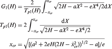
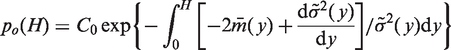
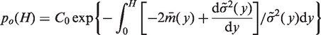
Suppose that the adjoint process $λ (t)$ depends on time t only via system energy H, then $λ (H)$ satisfies the following equation

\frac{1}{2} \tilde{σ} 2 \frac{d 2 λ}{d H 2} + [\tilde{m} - 4 b \frac{x_{cr}}{T_{p}} + \frac{λ}{2 R} (G - G_{1}) + \frac{1}{2} \frac{\partial \tilde{σ} 2}{\partial H}] \frac{d λ}{d H} + [\frac{\partial \tilde{m}}{\partial H} - \frac{4 b}{T_{p}^{2}} (T_{p} \frac{\partial x_{cr}}{\partial H} - x_{cr} \frac{\partial T_{p}}{\partial H})] λ + \frac{1}{4 R} (\frac{\partial G}{\partial H} - \frac{\partial G_{1}}{\partial H}) λ 2 - \frac{Rb 2}{T_{p}^{2}} (T_{p} \frac{\partial T_{p 1}}{\partial H} - T_{p 1} \frac{\partial T_{p}}{\partial H}) - \frac{\partial f}{\partial H} = 0

(33)

The Fokker-Planck-Kolmogorov (FPK) equation associated with the Itô equation (30) is (Zhu et al., 1997)

\frac{\partial p (H, t)}{\partial t} = - \frac{\partial [\bar{m} (H) p (H, t)]}{\partial H} + \frac{\partial 2 [\tilde{σ} 2 (H) p (H, t)]}{2 \partial H 2}

(34)

where p is the probability density of the Hamiltonian and

\bar{m} (H) = \tilde{m} (H) - 4 b \frac{x_{cr} (H)}{T_{p} (H)} + \frac{λ (H)}{2 R} [G (H) - G_{1} (H)]

(35)

A stationary solution to FPK equation (34) is

p_{o} (H) = C_{0} \exp {- \int_{0}^{H} [- 2 \bar{m} (y) + \frac{d \tilde{σ} 2 (y)}{d y}] / \tilde{σ} 2 (y) d y}

(36)

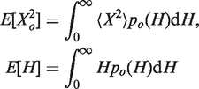
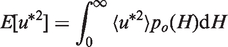
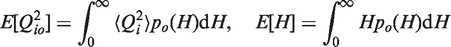
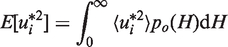
where C₀ is a normalization constant. The statistics of stochastic responses of the optimally controlled system can be calculated by using the probability density (36). For example, the mean square values of the controlled displacement and mean energy and the mean square value of the optimal control force are

E [X_{o}^{2}] = \int_{0}^{\infty} 〈 X 2 〉 p_{o} (H) d H, E [H] = \int_{0}^{\infty} {Hp}_{o} (H) d H

(37)

E [u * 2] = \int_{0}^{\infty} 〈 u * 2 〉 p_{o} (H) d H

(38)

Similarly, the statistics of stochastic responses of the uncontrolled system can be obtained in the same way by letting $u * = 0$ .

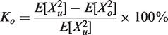
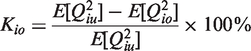
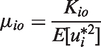
The performance of the proposed control strategy can be measured by criteria, i.e., the control effectiveness K_o and efficiency $μ_{o}$ (Zhu et al., 2001)

K_{o} = \frac{E [X_{u}^{2}] - E [X_{o}^{2}]}{E [X_{u}^{2}]} \times 100 %

(39)

μ_{o} = \frac{K_{o}}{E [u * 2]}

(40)

where

E [X_{u}^{2}]

is the mean square displacement of the uncontrolled system. K_o represents the percentage reduction in mean square displacements of the controlled system, and

μ_{o}

denotes the relative reduction per unit of the mean square control force. Obviously, higher K_o and

μ_{o}

indicate a better control strategy.

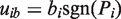
For comparison, the optimal bang–bang control strategy is also considered. The bang–bang control force for the quasi-integrable Hamiltonian system (24) is of the form (Ying and Zhu, 2006)

u_{b} = b sgn (\overset{\cdot}{X})

(41)

The statistics of stationary responses of the bang–bang controlled system can be calculated in a similar way to that for the optimally controlled system with $u *$ replaced by u_b.

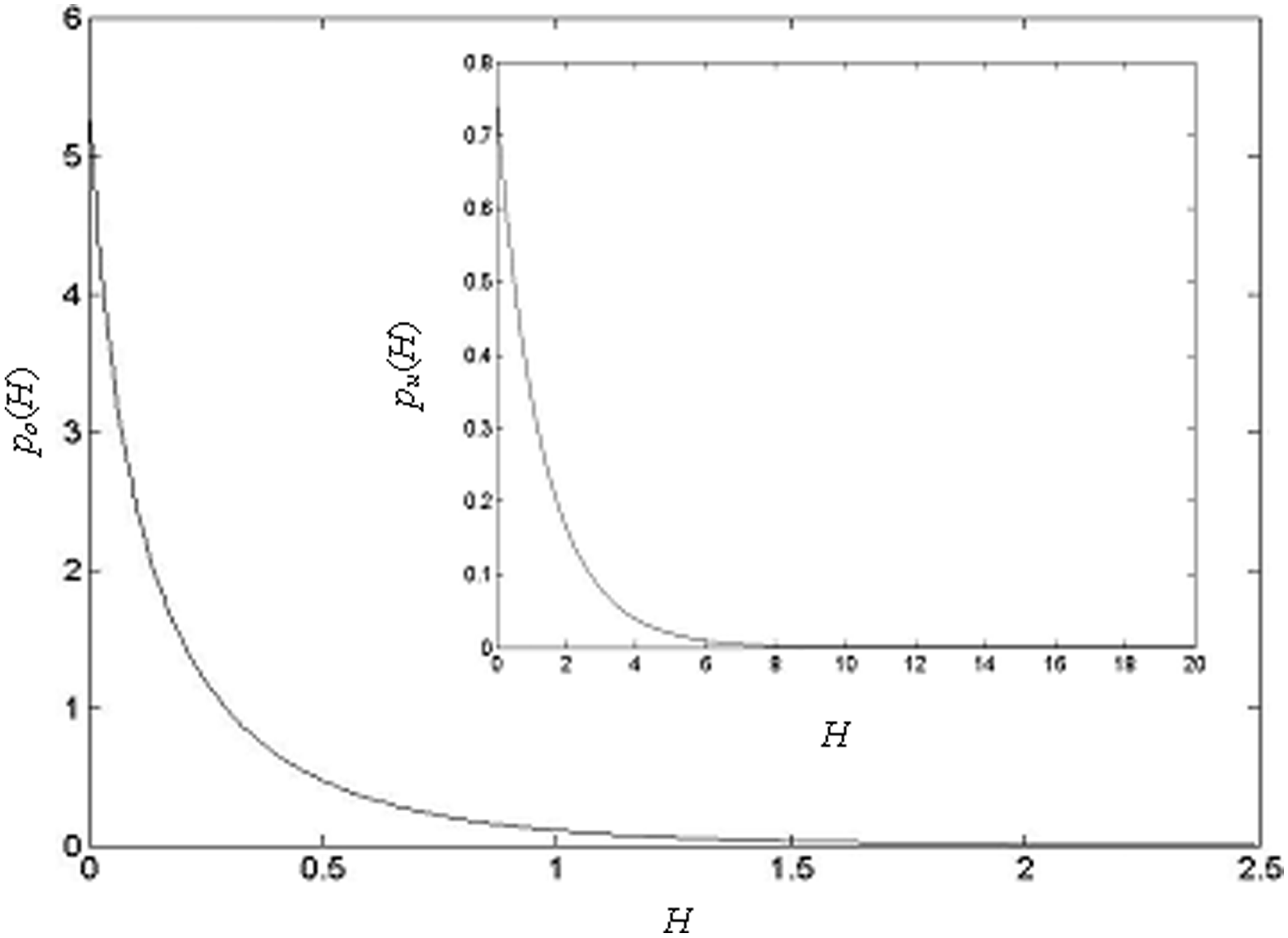
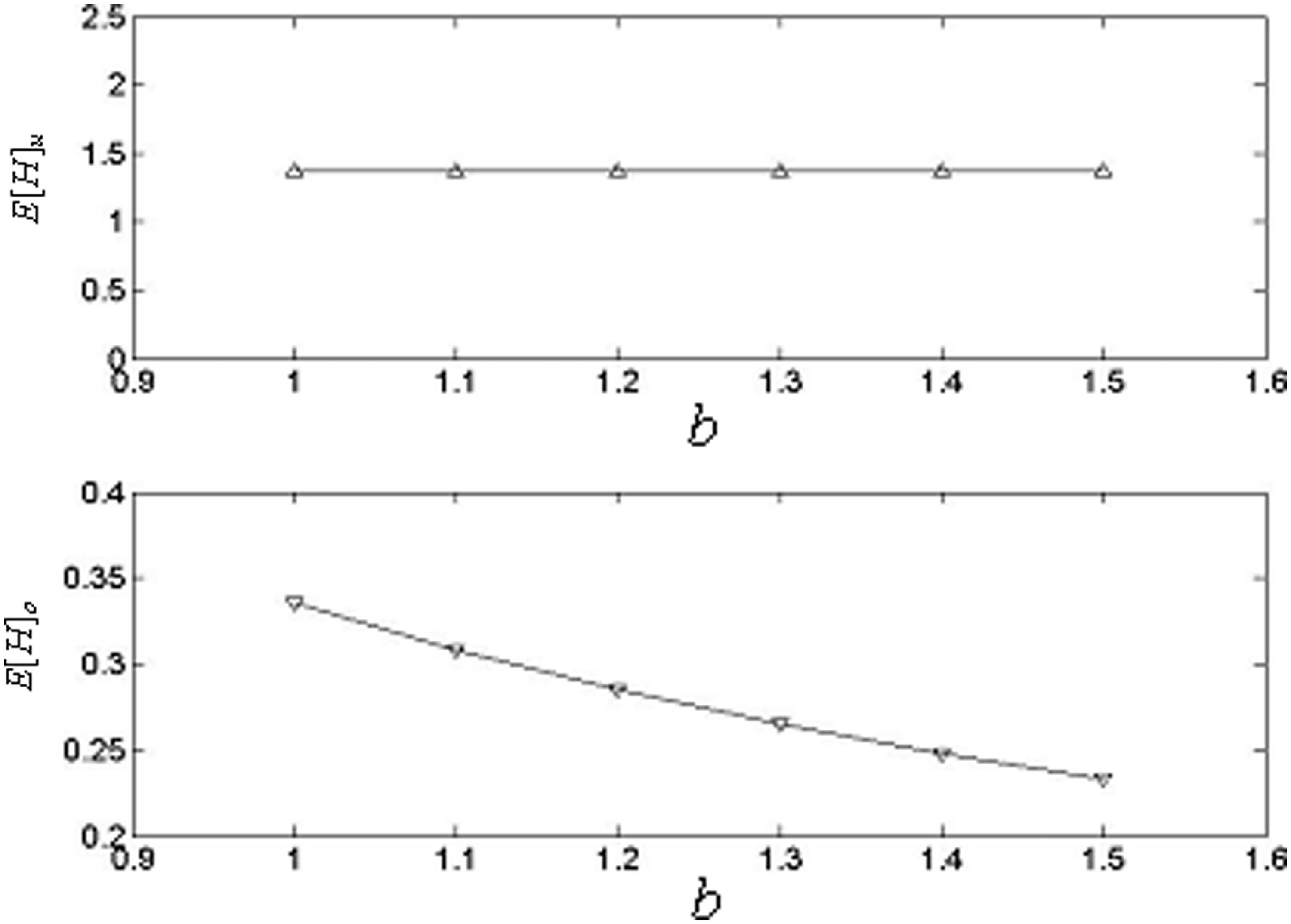
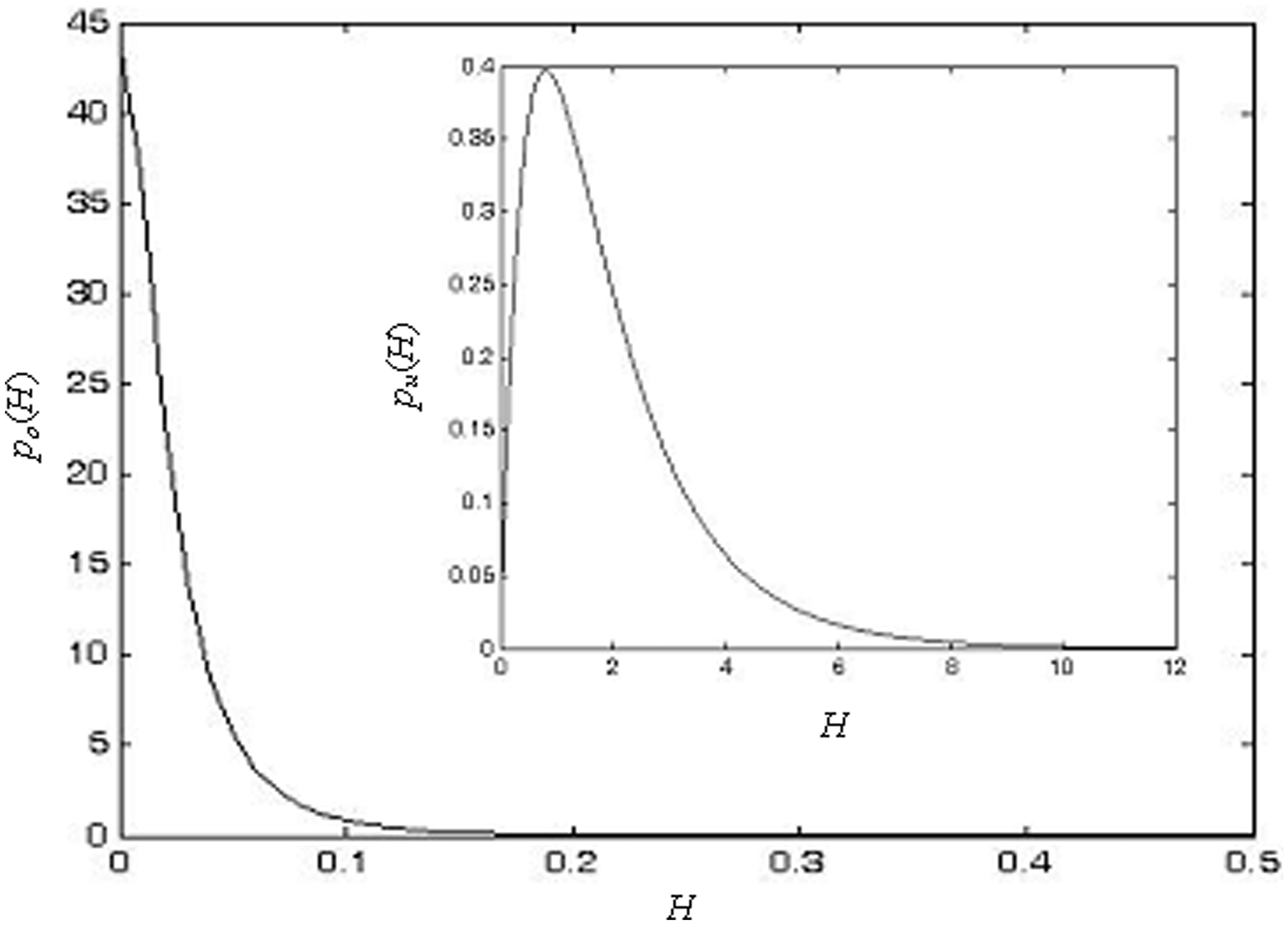
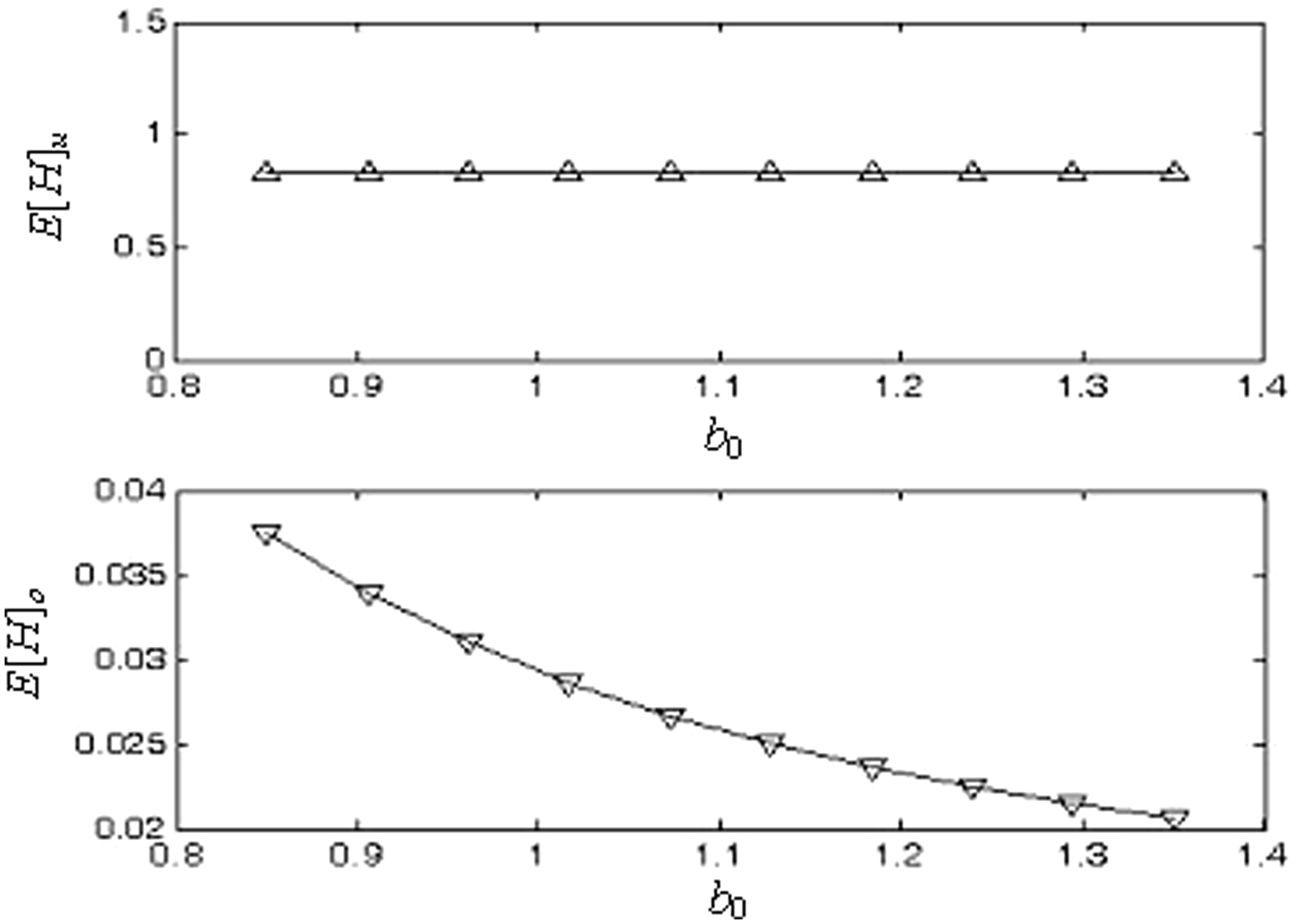
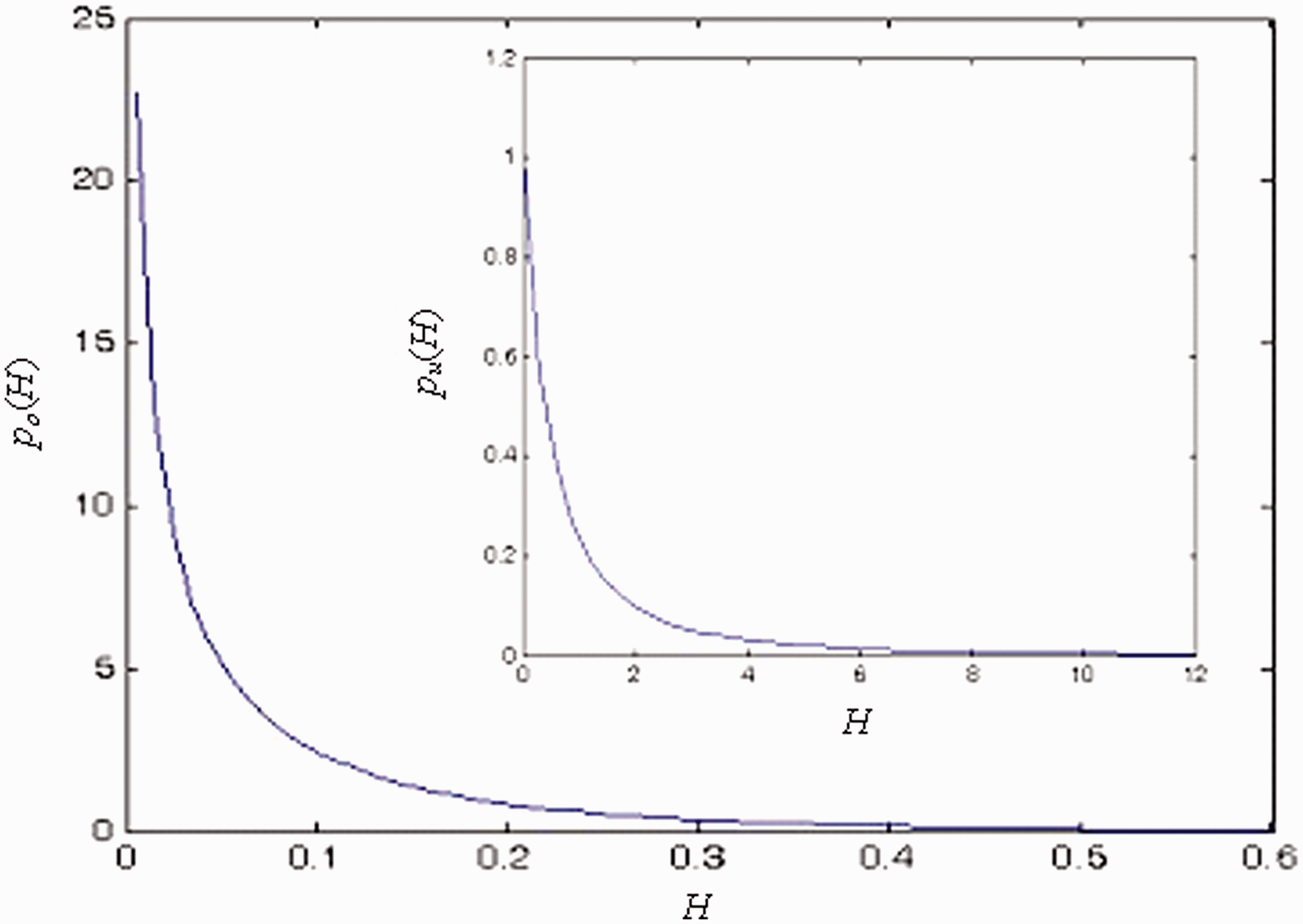
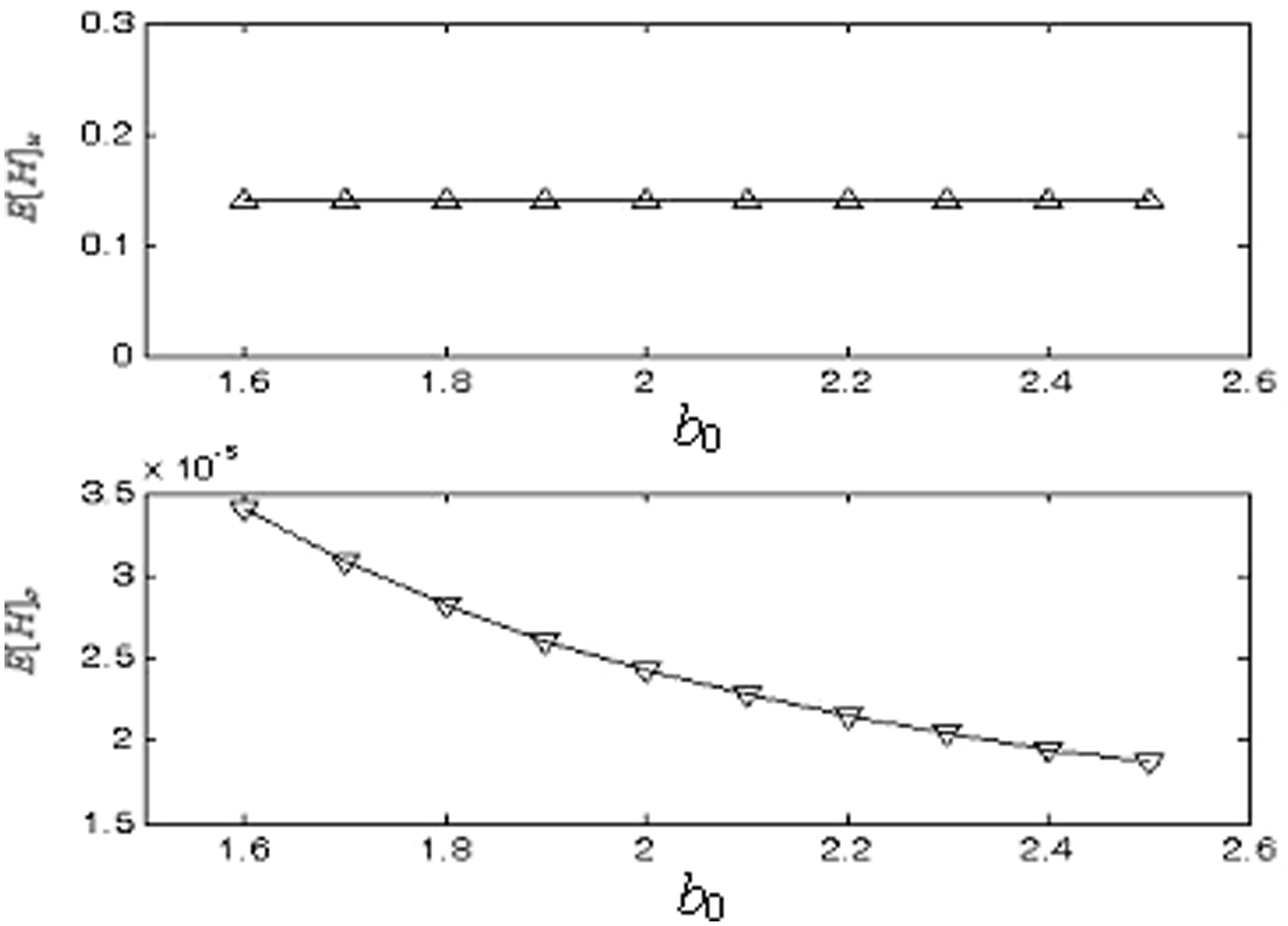
Numerical results are obtained and shown in Figures 1 –7 for the following parameter values: a = 1, e = 0.2, c = 0.2, D = 0.3, R = 0.6, s₁ = 0.0, s₂ = 1.5, s₃ = 0.0, λ(0) = −3.5, b = 1.2 unless otherwise mentioned. Figure 1 shows the stationary probability densities of energies (H) of the optimally controlled and uncontrolled systems (24). Figure 2 illustrates the remarkable reduction of mean energy of the optimally controlled system (E[H] _o ) compared with that of the uncontrolled system (E[H] _u ) for different control bounds (b).

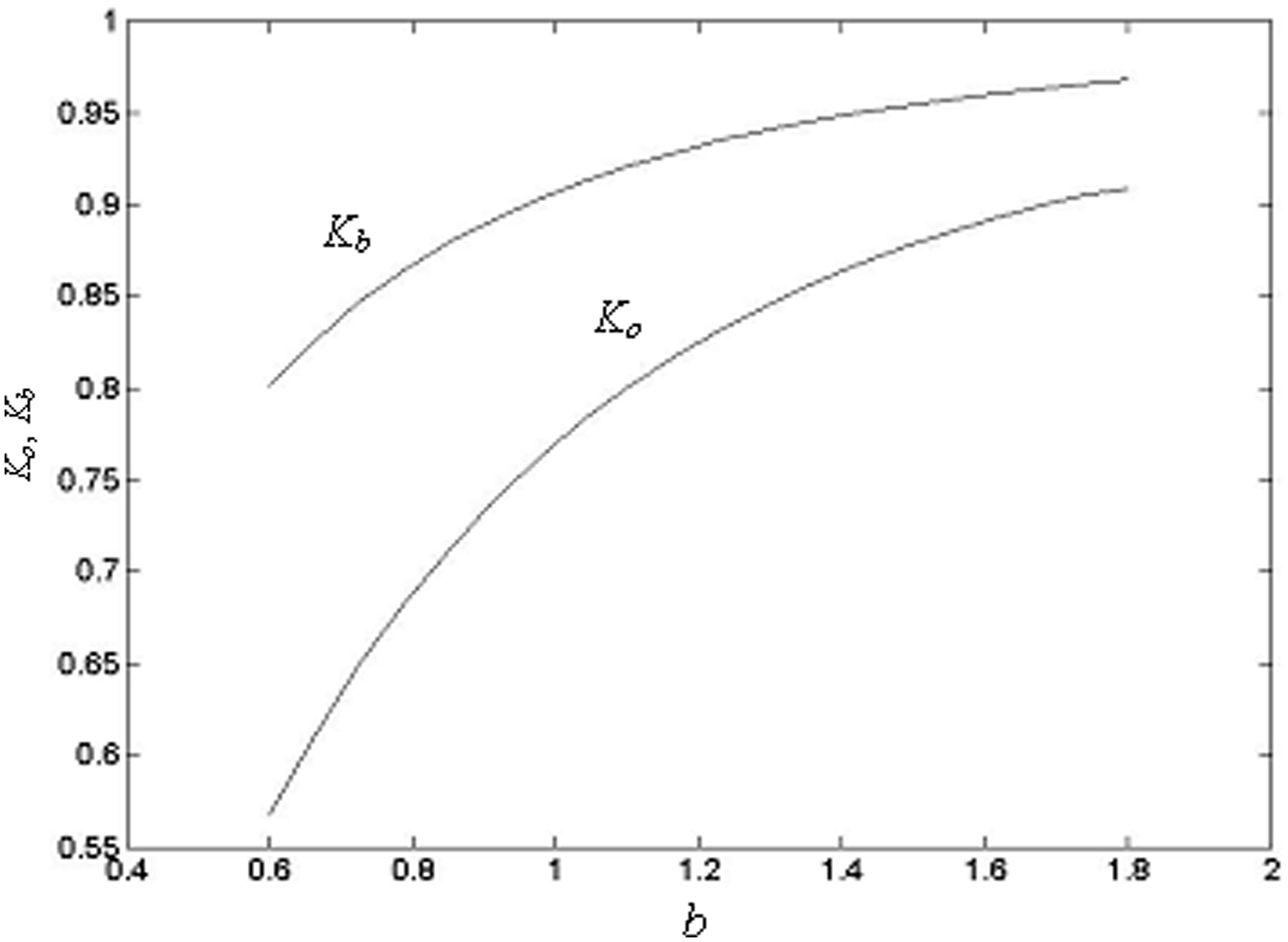
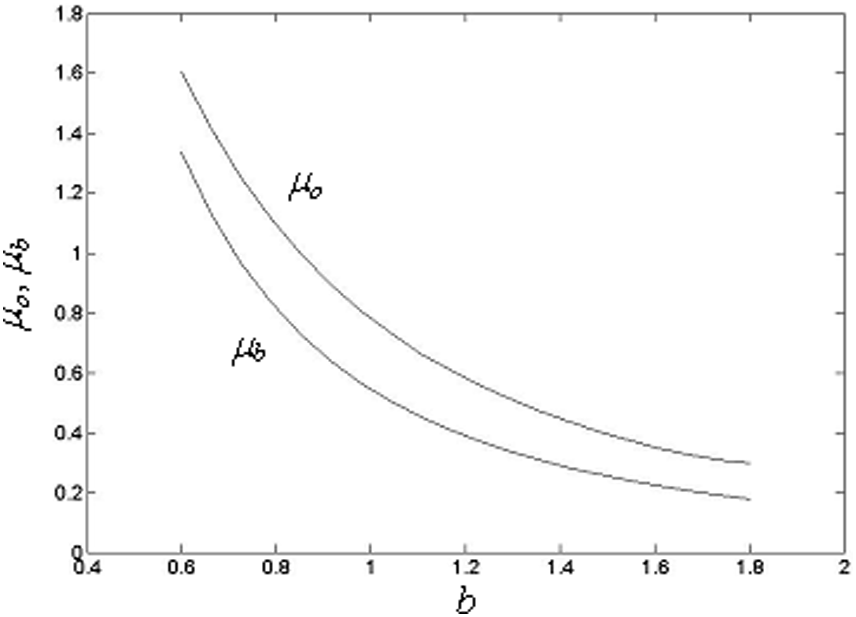
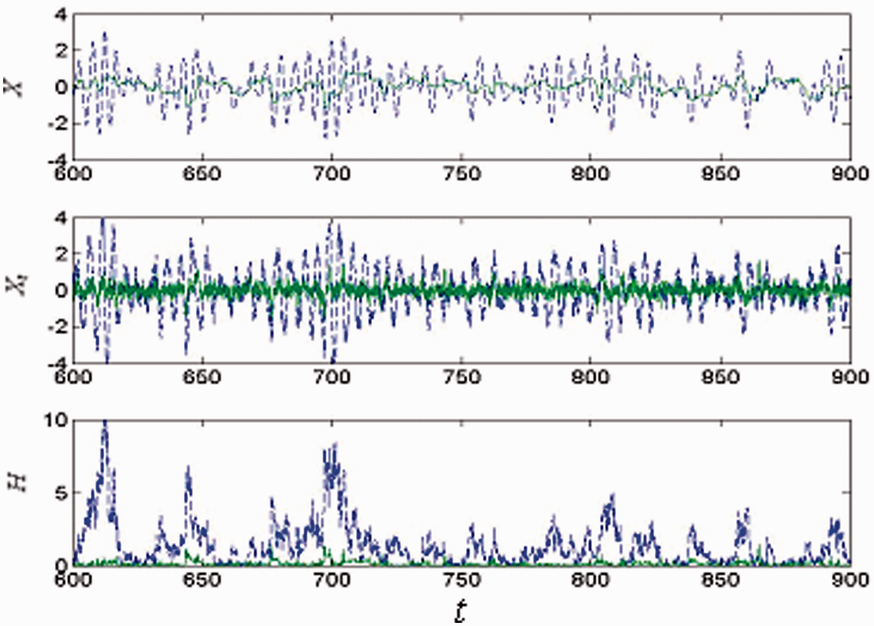
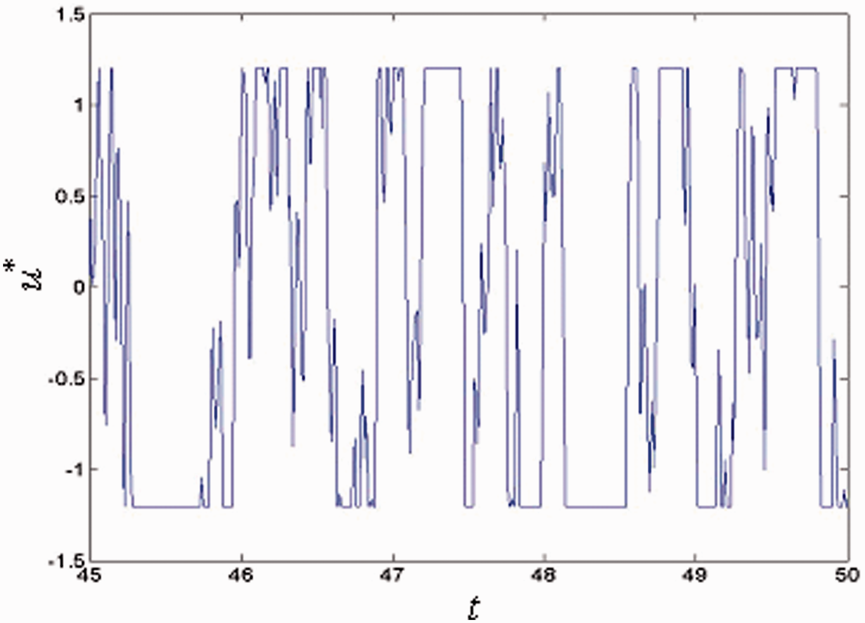
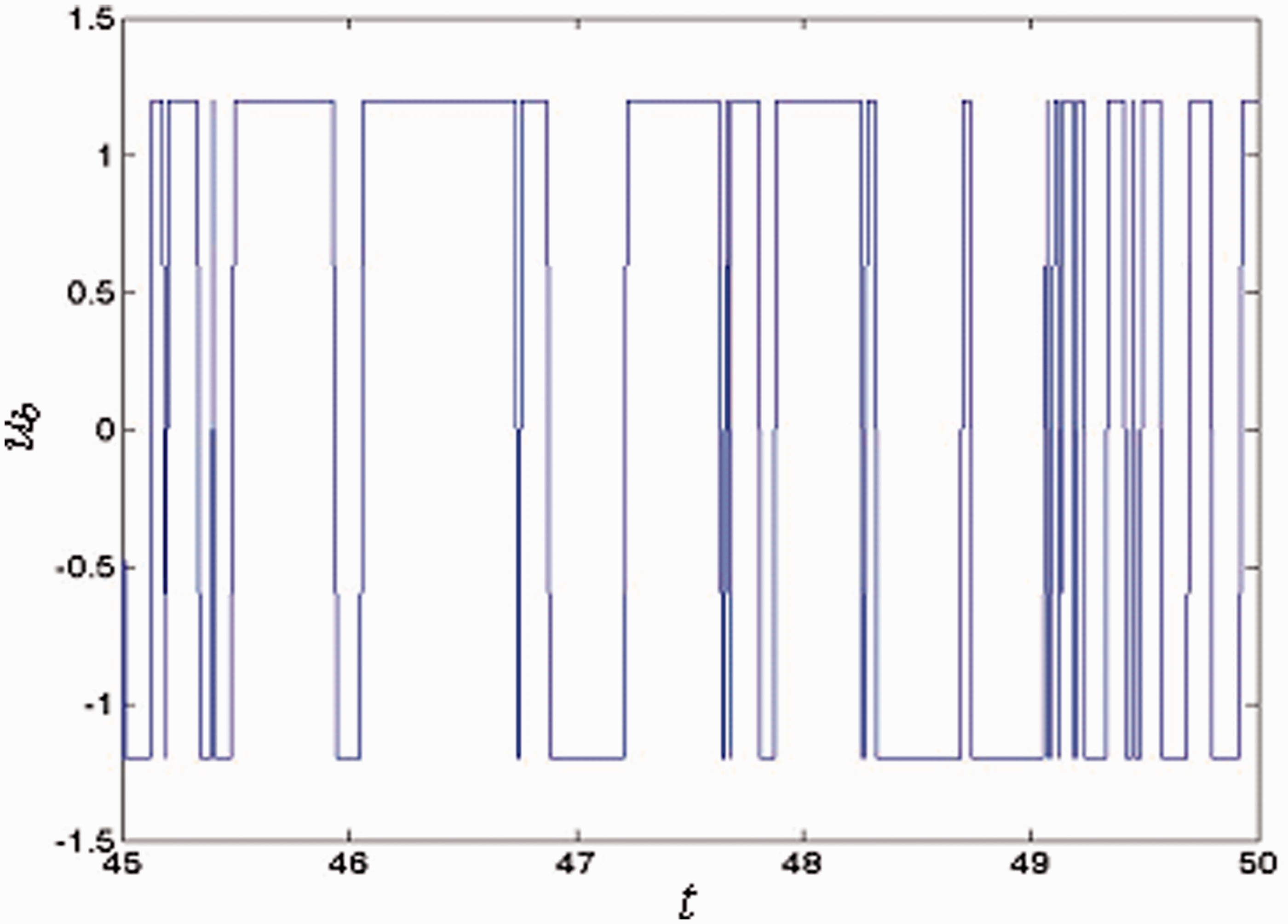
Figures 3 and 4 illustrate that the control effectiveness of the displacement response (X) increases with the control bound (b) and the control efficiency decreases correspondingly, respectively. For the bound b = 1.4, the control effectiveness of the proposed optimal bounded control K_o > 85% and the control efficiency μ_o > 0.4. Thus the proposed optimal bounded control strategy has high control effectiveness. It is seen by Figures 3 and 4 that the control effectiveness of the proposed optimal bounded control (K_o) is slightly less than that of the bang–bang control (K_b) for a large bound, and the control efficiency of the proposed optimal bounded control (μ_o) is higher than the bang-bang control (μ_b). Thus the proposed optimal bounded control strategy has high control efficiency. Figure 5 shows samples of the displacements (X), velocities (X_t) and energies (H) of the proposed controlled and uncontrolled systems (24), from which the effects of the optimal bounded control on the responses can be observed intuitively. Samples of the proposed optimal bounded control and bang–bang control are given in Figures 6 and 7, respectively. It is seen that the proposed optimal bounded control is less discontinuous than the bang–bang control. This means that the chattering is reduced in the proposed optimal bounded control strategy compared with the bang–bang control strategy.

Figure 1.

Stationary probability densities of energies (H) of the optimally controlled and uncontrolled systems (24): p_o(H) for the proposed optimal bounded control and p_u(H) for the non-control.

Figure 2.

Mean energies of system (24) as a function of the control bound (b): E[H] _o for the proposed optimal bounded control and E[H] _u for the non-control.

Figure 3.

Control effectiveness of the displacement response (X) of system (24) as a function of the control bound (b): K_o for the proposed optimal bounded control and K_b for the bang–bang control.

Figure 4.

Control efficiency of the displacement response (X) of system (24) as a function of the control bound (b): µ_o for the proposed optimal bounded control and µ_b for the bang–bang control.

Figure 5.

Samples of the displacement (X), velocity (X_t) and energy (H) of system (24): solid line for the proposed controlled system and dashed line for the uncontrolled system.

Figure 6.

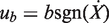
Sample of the proposed optimal bounded control force u* for the system (24).

Figure 7.

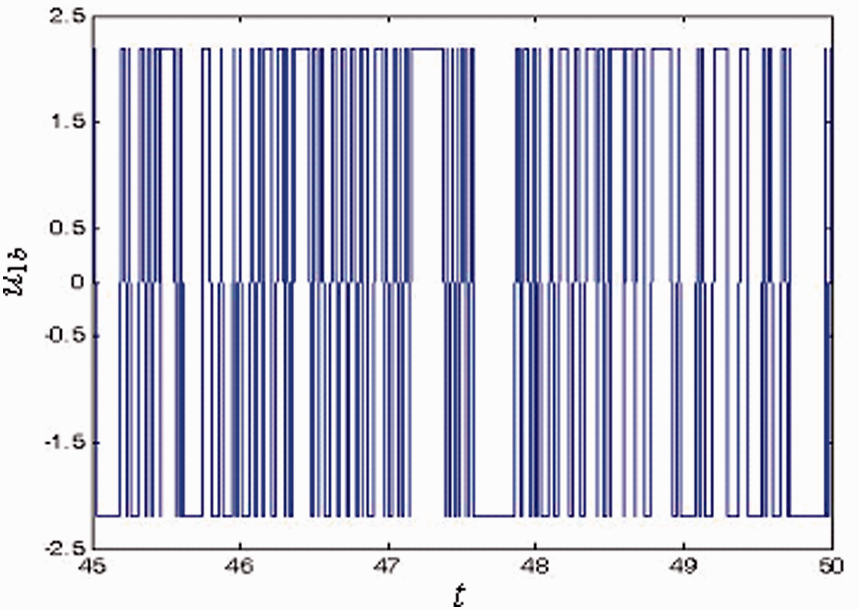
Sample of the bang–bang control force u_b for the system (24).

Figure 8.

Stationary probability densities of energies (H) of the optimally controlled and uncontrolled systems (42): p_o(H) for the proposed optimal bounded control and p_u(H) for the non-control.

Figure 9.

Mean energies of system (42) as a function of the control bound ( $b_{1} = b_{2} = b_{0}$ ): E[H] _o for the proposed optimal bounded control and E[H] _u for the non-control.

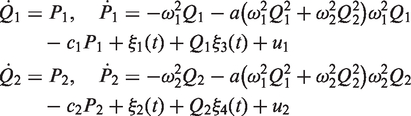
4.2. Nonlinearly coupled controlled Duffing oscillators

To illustrate the application and effectiveness of the proposed stochastic optimal bounded control strategy to a quasi-non-integrable Hamiltonian system, consider the following two controlled nonlinearly coupled Duffing oscillators

{\overset{\cdot}{Q}}_{1} = P_{1}, {\overset{\cdot}{P}}_{1} = - ω_{1}^{2} Q_{1} - a (ω_{1}^{2} Q_{1}^{2} + ω_{2}^{2} Q_{2}^{2}) ω_{1}^{2} Q_{1} - c_{1} P_{1} + ξ_{1} (t) + Q_{1} ξ_{3} (t) + u_{1} {\overset{\cdot}{Q}}_{2} = P_{2}, {\overset{\cdot}{P}}_{2} = - ω_{2}^{2} Q_{2} - a (ω_{1}^{2} Q_{1}^{2} + ω_{2}^{2} Q_{2}^{2}) ω_{2}^{2} Q_{2} - c_{2} P_{2} + ξ_{2} (t) + Q_{2} ξ_{4} (t) + u_{2}

(42)

where

ω_{1}

ω_{2}

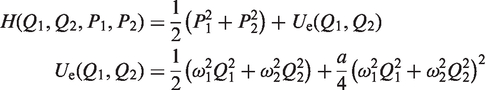
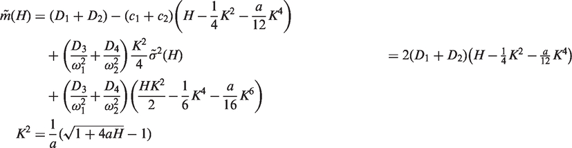
and a are positive constants; c₁ and c₂ are damping coefficients;

ξ_{k} (t)

(k = 1, 2, 3, 4) are independent Gaussian white noises with intensities

2 D_{k}

; u_i (i = 1, 2) are feedback control forces. The associated Hamiltonian is

H (Q_{1}, Q_{2}, P_{1}, P_{2}) = \frac{1}{2} (P_{1}^{2} + P_{2}^{2}) + U_{e} (Q_{1}, Q_{2}) U_{e} (Q_{1}, Q_{2}) = \frac{1}{2} (ω_{1}^{2} Q_{1}^{2} + ω_{2}^{2} Q_{2}^{2}) + \frac{a}{4} (ω_{1}^{2} Q_{1}^{2} + ω_{2}^{2} Q_{2}^{2}) 2

(43)

By applying the stochastic averaging method, the averaged Itô stochastic differential equation (2) is obtained with coefficients

\tilde{m} (H) = (D_{1} + D_{2}) - (c_{1} + c_{2}) (H - \frac{1}{4} K 2 - \frac{a}{12} K 4) + (\frac{D_{3}}{ω_{1}^{2}} + \frac{D_{4}}{ω_{2}^{2}}) \frac{K 2}{4} \tilde{σ} 2 (H) = 2 (D_{1} + D_{2}) (H - \frac{1}{4} K 2 - \frac{a}{12} K 4) + (\frac{D_{3}}{ω_{1}^{2}} + \frac{D_{4}}{ω_{2}^{2}}) (\frac{HK 2}{2} - \frac{1}{6} K 4 - \frac{a}{16} K 6) K 2 = \frac{1}{a} (\sqrt{1 + 4 aH} - 1)

(44)

The cost function is denoted by equation (7) with u = [u₁, u₂]^T, R = diag[R₁, R₂] and

f (H) = s_{0} + s_{1} H + s_{2} H 2 + s_{3} H 3

(45)

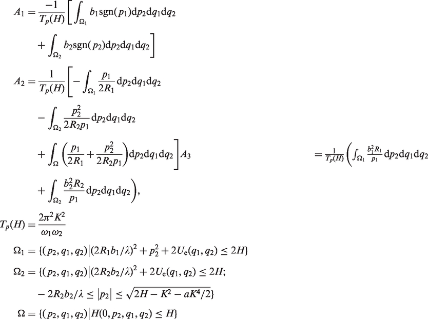
According to the stochastic maximum principle, the optimal bounded control forces are obtained as

u_{i}^{*} = {\frac{λ}{2 R_{i}} P_{i}, | \frac{λ}{2 R_{i}} P_{i} | < b_{i} b_{i} sgn (λ P_{i}), | \frac{λ}{2 R_{i}} P_{i} | \geq b_{i}

(46)

Substituting the control forces (46) into equations (11) and (12) yields the following forward-backward stochastic differential equations

d H = [\tilde{m} (H) + A_{1} + A_{2} λ (t)] d t + \tilde{σ} (H) d B (t) H (0) = H_{0}

(47)

d λ (t) = {- [\frac{\partial \tilde{m} (H)}{\partial H} + \frac{\partial A_{1}}{\partial H}] λ (t) - \frac{\partial \tilde{σ} (H)}{\partial H} κ (t) - \frac{1}{2} \frac{\partial A_{2}}{\partial H} λ 2 (t) + \frac{\partial A_{3}}{\partial H} + \frac{\partial f (H)}{\partial H}} d t + κ (t) d B (t) λ (T) = - \frac{\partial h (H (T))}{\partial H}

(48)

where

A_{1} = \frac{- 1}{T_{p} (H)} [\int_{Ω_{1}} b_{1} sgn (p_{1}) d p_{2} d q_{1} d q_{2} + \int_{Ω_{2}} b_{2} sgn (p_{2}) d p_{2} d q_{1} d q_{2}] A_{2} = \frac{1}{T_{p} (H)} [- \int_{Ω_{1}} \frac{p_{1}}{2 R_{1}} d p_{2} d q_{1} d q_{2} - \int_{Ω_{2}} \frac{p_{2}^{2}}{2 R_{2} p_{1}} d p_{2} d q_{1} d q_{2} + \int_{Ω} (\frac{p_{1}}{2 R_{1}} + \frac{p_{2}^{2}}{2 R_{2} p_{1}}) d p_{2} d q_{1} d q_{2}] A_{3} = \frac{1}{T_{p} (H)} (\int_{Ω_{1}} \frac{b_{1}^{2} R_{1}}{p_{1}} d p_{2} d q_{1} d q_{2} + \int_{Ω_{2}} \frac{b_{2}^{2} R_{2}}{p_{1}} d p_{2} d q_{1} d q_{2}), T_{p} (H) = \frac{2 π 2 K 2}{ω_{1} ω_{2}} Ω_{1} = {(p_{2}, q_{1}, q_{2}) | (2 R_{1} b_{1} / λ) 2 + p_{2}^{2} + 2 U_{e} (q_{1}, q_{2}) \leq 2 H} Ω_{2} = {(p_{2}, q_{1}, q_{2}) | (2 R_{2} b_{2} / λ) 2 + 2 U_{e} (q_{1}, q_{2}) \leq 2 H; - 2 R_{2} b_{2} / λ \leq | p_{2} | \leq \sqrt{2 H - K 2 - aK 4 / 2}} Ω = {(p_{2}, q_{1}, q_{2}) | H (0, p_{2}, q_{1}, q_{2}) \leq H}

(49)

Suppose that the adjoint process $λ (t)$ depends on time t only via system energy H, then $λ (H)$ satisfies the following equation

\frac{1}{2} \tilde{σ} 2 \frac{d 2 λ}{d H 2} + (\tilde{m} + A_{1} + A_{2} λ + \frac{1}{2} \frac{\partial \tilde{σ} 2}{\partial H}) \frac{d λ}{d H} + (\frac{\partial \tilde{m}}{\partial H} + \frac{\partial A_{1}}{\partial H}) λ + \frac{1}{2} \frac{\partial A_{2}}{\partial H} λ 2 - \frac{\partial A_{3}}{\partial H} - \frac{\partial f}{\partial H} = 0

(50)

The FPK equation associated with the Itô equation (47) is (Zhu and Yang, 1997)

\frac{\partial p (H, t)}{\partial t} = - \frac{\partial [\bar{m} (H) p (H, t)]}{\partial H} + \frac{\partial 2 [\tilde{σ} 2 (H) p (H, t)]}{2 \partial H 2}

(51)

where p is the probability density of the Hamiltonian and

\bar{m} (H) = \tilde{m} (H) + A_{1} + A_{2} λ (H)

(52)

A stationary solution to FPK equation (51) is

p_{o} (H) = C_{0} \exp {- \int_{0}^{H} [- 2 \bar{m} (y) + \frac{d \tilde{σ} 2 (y)}{d y}] / \tilde{σ} 2 (y) d y}

(53)

where C₀ is a normalization constant. The statistics of stochastic responses of the optimally controlled system can be calculated by using the probability density (53). For example, the mean square values of the controlled displacements and mean energy and the mean square values of the optimal control forces are

E [Q_{io}^{2}] = \int_{0}^{\infty} 〈 Q_{i}^{2} 〉 p_{o} (H) d H, E [H] = \int_{0}^{\infty} {Hp}_{o} (H) d H

(54)

E [u_{i}^{* 2}] = \int_{0}^{\infty} 〈 u_{i}^{* 2} 〉 p_{o} (H) d H

(55)

Similarly, the statistics of stochastic responses of the uncontrolled system can be obtained in the same way by letting $u_{i}^{*} = 0$ .

The performance of the proposed control strategy can be measured by the control effectiveness $K_{io}$ and efficiency $μ_{io}$

K_{io} = \frac{E [Q_{iu}^{2}] - E [Q_{io}^{2}]}{E [Q_{iu}^{2}]} \times 100 %

(56)

μ_{io} = \frac{K_{io}}{E [u_{i}^{* 2}]}

(57)

where

E [Q_{iu}^{2}]

are the mean square displacements of the uncontrolled system.

K_{io}

represent the percentage reductions in mean square displacements of the controlled system, and

μ_{io}

denote the relative reductions per unit of the mean square control forces.

The optimal bang–bang control strategy is also considered and the bang–bang control forces for the quasi-non-integrable Hamiltonian system (42) are of the form (Ying and Zhu, 2006)

u_{ib} = b_{i} sgn (P_{i})

(58)

The statistics of stationary responses of the bang–bang controlled system can be calculated in a similar way.

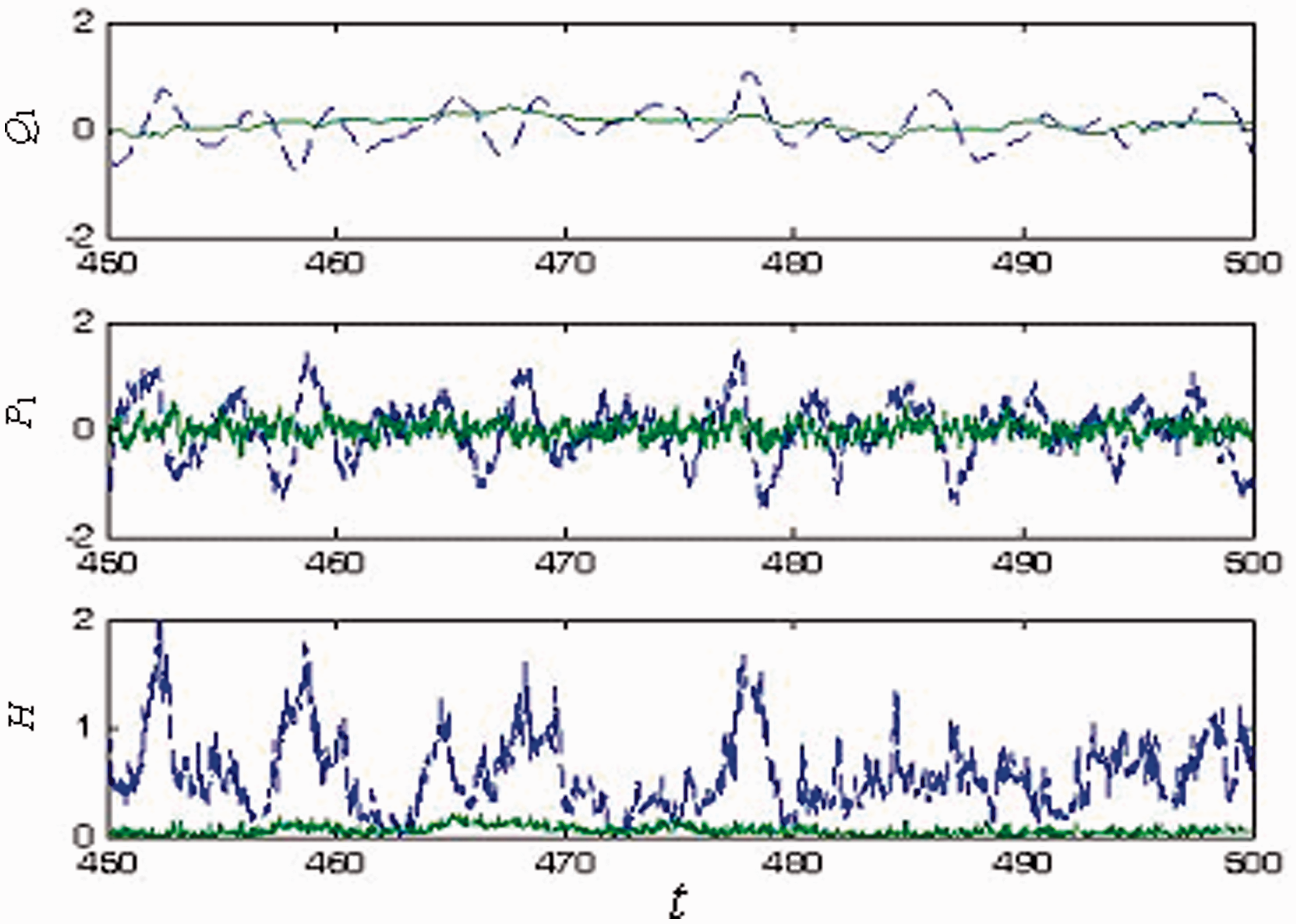
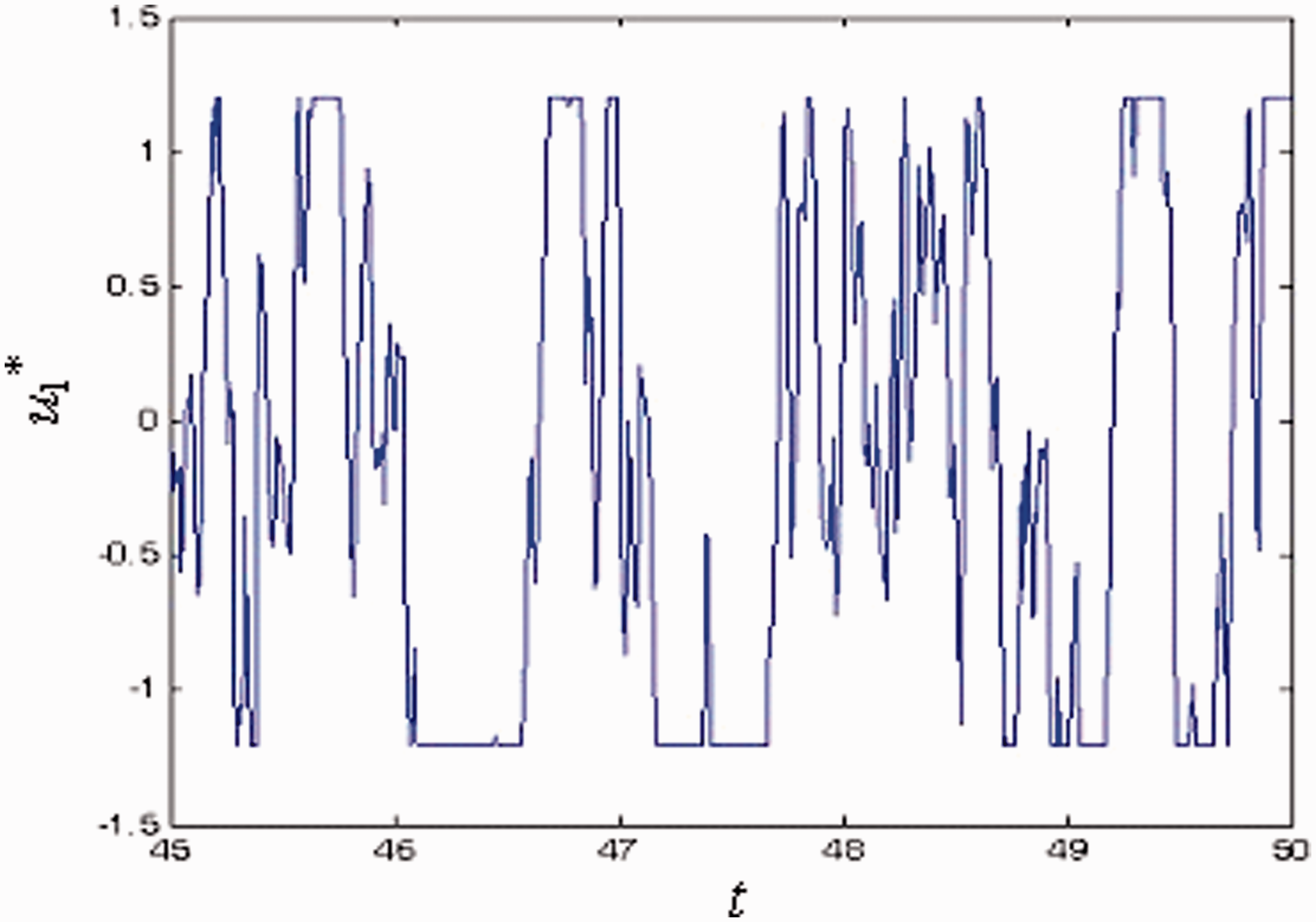
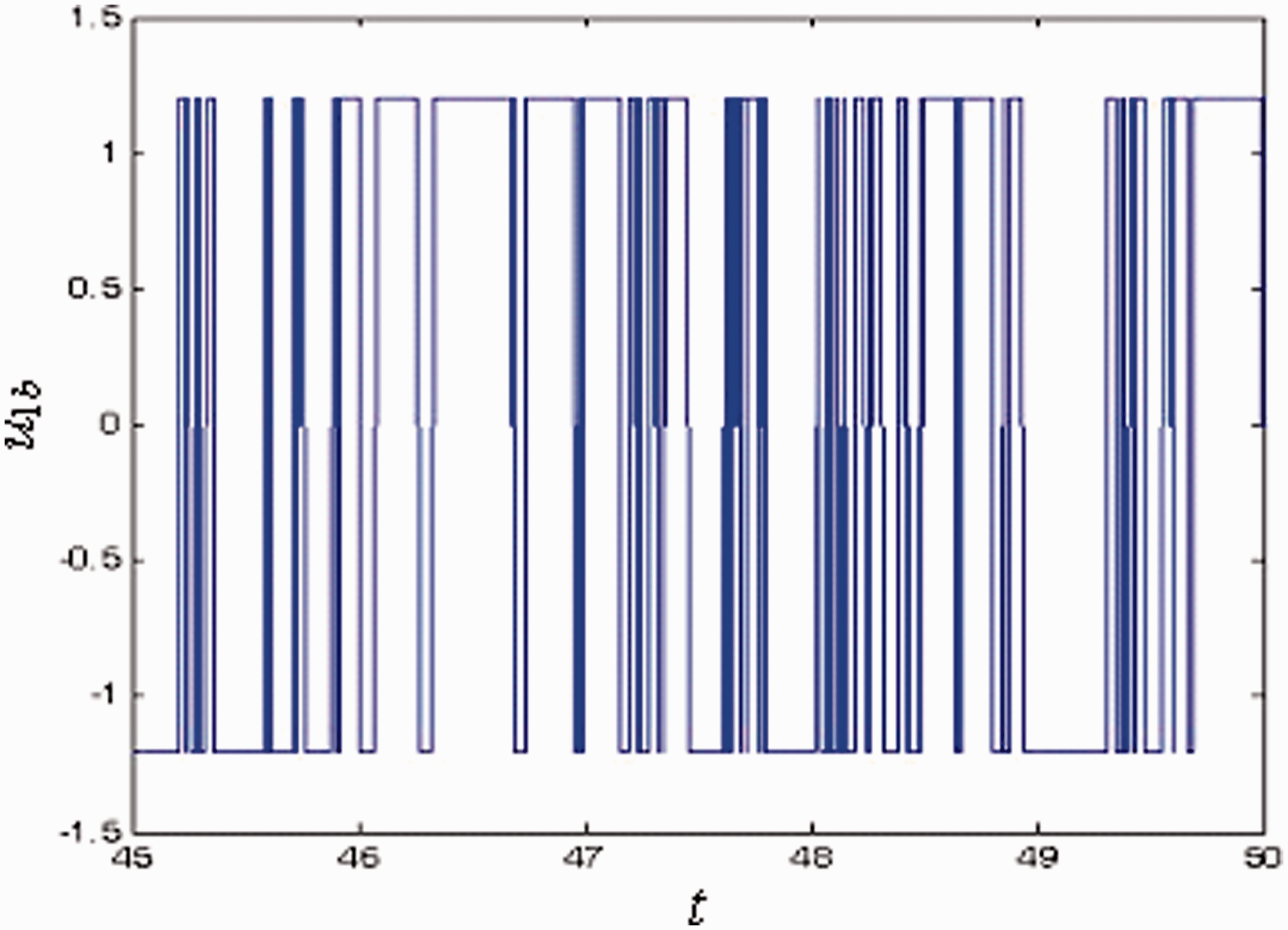
Numerical results are obtained and shown in Figures 8 –16 for the following parameter values: a = 2, ω₁ = 1.0, ω₂ = 1.414, c₁ = 0.2, c₂ = 0.3, D₁ = 0.1, D₂ = 0.08, D₃ = 0.4, D₄ = 0.36, R₁ = R₂ = 0.2, s₁ = 0.0, s₂ = 1.5, s₃ = 0.0, λ(0) = −3.4, b₁ = b₂ = 1.2 unless otherwise mentioned. Figure 8 shows the stationary probability densities of energies (H) of the optimally controlled and uncontrolled systems (42). Figure 9 illustrates the remarkable reduction of mean energy of the optimally controlled system (E[H] _o ) compared with that of the uncontrolled system (E[H] _u ) for different control bounds ( $b_{1} = b_{2} = b_{0}$ ). Figures 10 and 11 illustrate that the control effectiveness of the first displacement (Q₁) increases with the control bound ( $b_{1} = b_{2} = b_{0}$ ) and the control efficiency decreases correspondingly, respectively. For the bound b₀ = 1, the control effectiveness of the proposed optimal bounded control K_io > 94% and the control efficiency μ_io > 1.7. Thus the proposed optimal bounded control strategy has high control effectiveness. Figures 12 and 13 illustrate that the control effectiveness and control efficiency of the first displacement (Q₁) vary with the excitation intensity ( $D_{1} = D_{2} = D_{0}$ ), respectively. It is seen by Figures 10 and 12 that the control effectiveness of the proposed optimal bounded control ( $K_{1 o}$ ) is slightly less than that of the bang–bang control ( $K_{1 b}$ ). However, as shown in Figures 11 and 13, the control efficiency of the proposed optimal bounded control ( $μ_{io}$ ) is much higher than the bang-bang control ( $μ_{ib}$ ). Thus the proposed optimal bounded control strategy has high control efficiency. Figure 14 shows samples of the displacements (Q₁), velocities (P₁) and energies (H) of the proposed controlled and uncontrolled systems (42), which are used for intuitively observing the effects of the optimal bounded control on the responses. Samples of the proposed optimal bounded control and bang–bang control are given in Figures 15 and 16, respectively. It is seen that the proposed optimal bounded control is less discontinuous than the bang–bang control. Then the chattering is reduced in the proposed optimal bounded control strategy compared with the bang–bang control strategy.

Figure 10.

Control effectiveness of the first displacement (Q₁) of system (42) as a function of the control bound ( $b_{1} = b_{2} = b_{0}$ ): $K_{1 o}$ for the proposed optimal bounded control and $K_{1 b}$ for the bang–bang control.

Figure 11.

Control efficiency of the first displacement (Q₁) of system (42) as a function of the control bound ( $b_{1} = b_{2} = b_{0}$ ): $μ_{1 o}$ for the proposed optimal bounded control and $μ_{1 b}$ for the bang–bang control.

Figure 12.

Control effectiveness of the first displacement (Q₁) of system (42) as a function of the excitation intensity ( $D_{1} = D_{2} = D_{0}$ ): $K_{1 o}$ for the proposed optimal bounded control and $K_{1 b}$ for the bang–bang control.

Figure 13.

Control efficiency of the first displacement (Q₁) of system (42) as a function of the excitation intensity ( $D_{1} = D_{2} = D_{0}$ ): $μ_{1 o}$ for the proposed optimal bounded control and $μ_{1 b}$ for the bang–bang control.

Figure 14.

Samples of the displacement (Q₁), velocity (P₁) and energy (H) of system (42): solid line for the proposed controlled system and dashed line for the uncontrolled system.

Figure 15.

Sample of the proposed optimal bounded control force $u_{1}^{*}$ for the first degree-of-freedom of system (42).

Figure 16.

Sample of the bang–bang control force $u_{1 b}$ for the first degree-of-freedom of system (42).

4.3. Nonlinear controlled cable structure

To illustrate the further application of the proposed stochastic optimal bounded control strategy, consider the following controlled nonlinear cable structure. The differential equations of transverse motion of the controlled inclined stay cable can be expressed as (Ying et al., 2007)

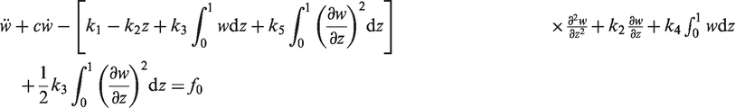
m {\overset{··}{v}}_{1} + c_{v} {\overset{\cdot}{v}}_{1} = (T_{0} + EA ɛ) \frac{\partial 2 v_{1}}{\partial s 2} + \frac{d T_{0}}{d s} \frac{\partial v_{1}}{\partial s} + EA ɛ \frac{d 2 n_{1}}{d s 2} + f_{2}

(59)

where v₁ is the transverse displacement of the cable; m is the mass per unit of cable length; c_v is the damping coefficient; T₀ is the cable tension in static equilibrium; E is the elastic modulus; A is the cross-sectional area of the cable; ɛ is the longitudinal strain; s is the curvilinear coordinate; n₁ is the unit normal vector of the cable curve; f₂ is the external and control force. The boundary conditions of the cable with two fixed ends are v₁ = 0 for s = 0, L_c, where L_c is the cable length. By using the expressions of nonlinear strain, tension and static equilibrium configuration, the differential equation for the transverse vibration of the cable can be obtained in the dimensionless form as follows

\overset{··}{w} + c \overset{\cdot}{w} - [k_{1} - k_{2} z + k_{3} \int_{0}^{1} w d z + k_{5} \int_{0}^{1} (\frac{\partial w}{\partial z}) 2 d z] \times \frac{\partial 2 w}{\partial z 2} + k_{2} \frac{\partial w}{\partial z} + k_{4} \int_{0}^{1} w d z + \frac{1}{2} k_{3} \int_{0}^{1} (\frac{\partial w}{\partial z}) 2 d z = f_{0}

(60)

where

w = \frac{v_{1}}{L_{c}}, z = \frac{s}{L_{c}}, c = \frac{c_{v}}{m}, f_{0} = \frac{f_{2}}{mL}, k_{1} = \frac{T_{x}}{{mL}_{c}^{2} \sin α} + \frac{k_{2}}{2} k_{2} = \frac{g \cos α}{L_{c} \sin 2 α}, k_{3} = \frac{EAg}{T_{x} L_{c}}, k_{4} = \frac{EA}{m} (\frac{mg}{T_{x}}) 2, k_{5} = \frac{EA}{2 {mL}_{c}^{2}}

(61)

in which T_x is the horizontal static tension; α is the inclined angle of the cable. The boundary conditions become w = 0 for z = 0,1.

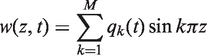
Based on the boundary conditions, the non-dimensional displacement w is expanded as

w (z, t) = \sum_{k = 1}^{M} q_{k} (t) \sin k π z

(62)

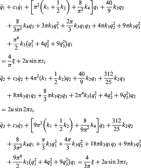
where q_k are generalized displacements. According to the Galerkin method, substituting displacement (62) into equation (60) and using the orthogonality relations of harmonic functions yield ordinary differential equations for q_i. The first three equations are

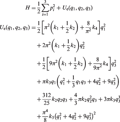
{\overset{··}{q}}_{1} + c_{1} {\overset{\cdot}{q}}_{1} + [π 2 (k_{1} + \frac{1}{2} k_{2}) + \frac{8}{π 2} k_{4}] q_{1} + \frac{40}{9} k_{2} q_{2} + \frac{8}{3 π 2} k_{4} q_{3} + 3 π k_{3} q_{1}^{2} + \frac{2 π}{3} k_{3} q_{1} q_{3} + 4 π k_{3} q_{2}^{2} + 9 π k_{3} q_{3}^{2} + \frac{π 4}{2} k_{5} (q_{1}^{2} + 4 q_{2}^{2} + 9 q_{3}^{2}) q_{1} = \frac{4}{π} ξ + 2 u \sin π z_{c} {\overset{··}{q}}_{2} + c_{2} {\overset{\cdot}{q}}_{2} + 4 π 2 (k_{1} + \frac{1}{2} k_{2}) q_{2} + \frac{40}{9} k_{2} q_{1} + \frac{312}{25} k_{2} q_{3} + 8 π k_{3} q_{1} q_{2} + \frac{8}{3} π k_{3} q_{2} q_{3} + 2 π 4 k_{5} (q_{1}^{2} + 4 q_{2}^{2} + 9 q_{3}^{2}) q_{2} = 2 u \sin 2 π z_{c} {\overset{··}{q}}_{3} + c_{3} {\overset{\cdot}{q}}_{3} + [9 π 2 (k_{1} + \frac{1}{2} k_{2}) + \frac{8}{9 π 2} k_{4}] q_{3} + \frac{312}{25} k_{2} q_{2} + \frac{8}{3 π 2} k_{4} q_{1} + \frac{π}{3} k_{3} q_{1}^{2} + \frac{4 π}{3} k_{3} q_{2}^{2} + 18 π k_{3} q_{1} q_{3} + 9 π k_{3} q_{3}^{2} + \frac{9 π 4}{2} k_{5} (q_{1}^{2} + 4 q_{2}^{2} + 9 q_{3}^{2}) q_{1} = \frac{4}{3 π} ξ + 2 u \sin 3 π z_{c}

(63)

where c_i = 2ζ_iω_i; ζ_i are damping ratios;

ω_{i} = i π \sqrt{k_{1} + k_{2} / 2}

(i = 1, 2, 3); z_c denotes the place of control force u; ξ is the Gaussian white noise excitation. The associated Hamiltonian is

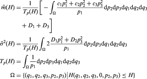
H = \frac{1}{2} \sum_{i = 1}^{3} p_{i}^{2} + U_{e} (q_{1}, q_{2}, q_{3}) U_{e} (q_{1}, q_{2}, q_{3}) = \frac{1}{2} [π 2 (k_{1} + \frac{1}{2} k_{2}) + \frac{8}{π 2} k_{4}] q_{1}^{2} + 2 π 2 (k_{1} + \frac{1}{2} k_{2}) q_{2}^{2} + \frac{1}{2} [9 π 2 (k_{1} + \frac{1}{2} k_{2}) + \frac{8}{9 π 2} k_{4}] q_{3}^{2} + π k_{3} q_{1} (q_{1}^{2} + \frac{1}{3} q_{1} q_{3} + 4 q_{2}^{2} + 9 q_{3}^{2}) + \frac{312}{25} k_{2} q_{2} q_{3} + \frac{4}{3} π k_{2} q_{2}^{2} q_{3} + 3 π k_{3} q_{3}^{3} + \frac{π 4}{8} k_{5} (q_{1}^{2} + 4 q_{2}^{2} + 9 q_{3}^{2}) 2

(64)

By applying the stochastic averaging method, the averaged Itô stochastic differential equation (2) is obtained with coefficients

\tilde{m} (H) = \frac{1}{T_{p} (H)} [- \int_{Ω} \frac{c_{1} p_{1}^{2} + c_{2} p_{2}^{2} + c_{3} p_{3}^{2}}{p_{1}} d p_{2} d p_{3} d q_{1} d q_{2} d q_{3} + D_{1} + D_{3}] \tilde{σ} 2 (H) = \frac{1}{T_{p} (H)} \int_{Ω} 2 \frac{D_{1} p_{1}^{2} + D_{2} p_{3}^{2}}{p_{1}} d p_{2} d p_{3} d q_{1} d q_{2} d q_{3} T_{p} (H) = \int_{Ω} \frac{1}{p_{1}} d p_{2} d p_{3} d q_{1} d q_{2} d q_{3} Ω = {(q_{1}, q_{2}, q_{3}, p_{2}, p_{3}) | H (q_{1}, q_{2}, q_{3}, 0, p_{2}, p_{3}) \leq H}

(65)

where D_i and u_i are the excitation intensities and controls corresponding to q_i, respectively.

The cost function is denoted by equation (7) with u = [u₁, u₂, u₃]^T, R = diag[R₁, R₂, R₃] and f(H) as given by equation (45). According to the stochastic maximum principle, the optimal bounded control forces are obtained as equation (46). Substituting the control forces into equations (11) and (12) yields the forward-backward stochastic differential equations. The adjoint process λ(H) satisfies the following equation

\frac{1}{2} \tilde{σ} 2 \frac{d 2 λ}{d H 2} + (\tilde{m} + A_{4} + A_{5} λ + \frac{1}{2} \frac{\partial \tilde{σ} 2}{\partial H}) \frac{d λ}{d H} + (\frac{\partial \tilde{m}}{\partial H} + \frac{\partial A_{4}}{\partial H}) λ + \frac{1}{2} \frac{\partial A_{5}}{\partial H} λ 2 - \frac{\partial A_{6}}{\partial H} - \frac{\partial f}{\partial H} = 0

(66)

where

A_{4} = \frac{- 1}{T_{p} (H)} [\int_{Ω_{1}} b_{1} sgn (p_{1}) d p_{2} d p_{3} d q_{1} d q_{2} d q_{3} + \int_{Ω_{2}} b_{2} sgn (p_{2}) d p_{2} d p_{3} d q_{1} d q_{2} d q_{3} + \int_{Ω_{3}} b_{3} sgn (p_{3}) d p_{2} d p_{3} d q_{1} d q_{2} d q_{3}] A_{5} = \frac{1}{T_{p} (H)} [- \int_{Ω_{1}} \frac{p_{1}}{2 R_{1}} d p_{2} d p_{3} d q_{1} d q_{2} d q_{3} - \int_{Ω_{2}} \frac{p_{2}^{2}}{2 R_{2} p_{1}} d p_{2} d p_{3} d q_{1} d q_{2} d q_{3} - \int_{Ω_{3}} \frac{p_{3}^{2}}{2 R_{3} p_{1}} d p_{2} d p_{3} d q_{1} d q_{2} d q_{3} + \int_{Ω} (\frac{p_{1}}{2 R_{1}} + \frac{p_{2}^{2}}{2 R_{2} p_{1}} + \frac{p_{3}^{2}}{2 R_{3} p_{1}}) d p_{2} d p_{3} d q_{1} d q_{2} d q_{3}] A_{6} = \frac{1}{T_{p} (H)} (\int_{Ω_{1}} \frac{b_{1}^{2} R_{1}}{p_{1}} d p_{2} d p_{3} d q_{1} d q_{2} d q_{3} + \int_{Ω_{2}} \frac{b_{2}^{2} R_{2}}{p_{1}} d p_{2} d p_{3} d q_{1} d q_{2} d q_{3} + \int_{Ω_{3}} \frac{b_{3}^{2} R_{3}}{p_{1}} d p_{2} d p_{3} d q_{1} d q_{2} d q_{3}) Ω_{1} = {(p_{2}, p_{3}, q_{1}, q_{2}, q_{3}) | (2 R_{1} b_{1} / λ) 2 + p_{2}^{2} + p_{3}^{2} + 2 U_{e} \leq 2 H} Ω_{2} = {(p_{2}, p_{3}, q_{1}, q_{2}, q_{3}) | (2 R_{2} b_{2} / λ) 2 + p_{3}^{2} + 2 U_{e} \leq 2 H; - 2 R_{2} b_{2} / λ \leq | p_{2} | \leq \sqrt{2 H - 2 U_{e}}} Ω_{3} = {(p_{2}, p_{3}, q_{1}, q_{2}, q_{3}) | (2 R_{2} b_{2} / λ) 2 + p_{2}^{2} + 2 U_{e} \leq 2 H; - 2 R_{2} b_{2} / λ \leq | p_{3} | \leq \sqrt{2 H - 2 U_{e}}}

(67)

Equation (66) for the adjoint process λ as a function of H is a deterministic ordinary differential equation. The deterministic function $λ (H)$ can be obtained by solving this equation, for example, using the Runge-Kutta algorithm for the infinite time control of free terminal with initial conditions corresponding to certain final values. Then the adjoint process is determined, and the optimal controls $u_{i}^{*}$ are determined by substituting the deterministic function $λ (H)$ into equation (46). The fully averaged Itô equation (12) is obtained by using the optimal controls and the FPK equation (51) is formed. The probability density (53) and the mean square responses of the optimally controlled system can be calculated for evaluating the control efficacy.

Numerical results are obtained and shown in Figures 17 –23 for the following parameter values: L_c = 130.0 m, A = 60.0 cm², m = 60.0 kg/m, E = 180 GPa, α = 0.984 rad, T_x = 4000sinα kN, ζ_i = 0.0005, D₁ = D₃ = 0.03, z_c = 0.9, R_i = 4.0siniπz_c, s₁ = 0.0, s₂ = 2.0, s₃ = 0.0, λ(0) = −2.8, b₁ = b₂ = b₃ = 2.2 (i = 1, 2, 3) unless otherwise mentioned. Figure 17 shows the stationary probability densities of energies (H) of the optimally controlled and uncontrolled cable structures (60). Figure 18 illustrates the great reduction of mean energy of the optimally controlled cable structure compared with that of the uncontrolled cable for different control bounds ( $b_{1} = b_{2} = b_{3} = b_{0}$ ). Figures 19 and 20 illustrate that the control effectiveness of the cable displacement (w) increases with the control bound ( $b_{1} = b_{2} = b_{3} = b_{0}$ ) and the control efficiency decreases correspondingly, respectively. For the bound b₀ = 2.2, the control effectiveness of the proposed optimal bounded control K_o > 89% and the control efficiency μ_o > 1.65. Thus the proposed optimal bounded control can achieve high control effectiveness and efficiency. Figure 21 shows samples of the displacements (w), velocities (w_t) and energies (H) of the proposed controlled and uncontrolled cable structures. Figures 22 and 23 show samples of the proposed optimal bounded control and bang–bang control, respectively. It is obtained that the proposed optimal bounded control strategy can reduce more chattering than the bang–bang control strategy.

Figure 17.

Stationary probability densities of energies (H) of the optimally controlled and uncontrolled cables: p_o(H) for the proposed optimal bounded control and p_u(H) for the non-control.

Figure 18.

Mean energies of cable structure as a function of the control bound ( $b_{1} = b_{2} = b_{3} = b_{0}$ ): E[H] _o for the proposed optimal bounded control and E[H] _u for the non-control.

Figure 19.

Control effectiveness of the cable displacement (w) as a function of the control bound ( $b_{1} = b_{2} = b_{3} = b_{0}$ ): $K_{o}$ for the proposed optimal bounded control and $K_{b}$ for the bang–bang control.

Figure 20.

Control efficiency of the cable displacement (w) as a function of the control bound ( $b_{1} = b_{2} = b_{3} = b_{0}$ ): $μ_{o}$ for the proposed optimal bounded control and $μ_{b}$ for the bang–bang control.

Figure 21.

Samples of the cable displacement (w), velocity (w_t) and energy (H): solid line for the proposed controlled structure and dashed line for the uncontrolled structure.

Figure 22.

Sample of the proposed optimal bounded control force $u_{1}^{*}$ for the first degree-of-freedom of cable.

Figure 23.

Sample of the bang–bang control force $u_{1 b}$ for the first degree-of-freedom of cable.

5. Conclusions

A nonlinear stochastic optimal bounded control strategy for quasi-Hamiltonian systems with actuator saturation has been proposed based on the stochastic averaging method and stochastic maximum principle. The proposed strategy combines the advantages of optimal unbounded control and bang–bang control, which has the high control effectiveness and efficiency, and the slight chattering effect compared with the bang-bang control strategy. By using the stochastic averaging method, the dimension of the control system is reduced and the system state control is transformed into the system energy control. The proposed control strategy is applicable to nonlinear multi degree-of-freedom structural systems under stochastic excitations and control devices with bounded forces.

Footnotes

Funding

This work was supported by the National Natural Science Foundation of China (grant numbers 10932009, 11072212, 11072215 and 11272279).

References

Bartolini

Punta

(2000) Chattering elimination with second-order sliding modes robust to coulomb friction. ASME Journal of Dynamic Systems, Measurement and Control 122: 679–686.

Bartoszewicz

(2000) Chattering attenuation in sliding mode control systems. Control and Cybernetics 29: 585–594.

Bratus

Dimentberg

Iourtchenko

(2000) Optimal bounded response control for a second-order system under a white-noise excitation. Journal of Vibration and Control 6: 741–755.

Crespo

Sun

(2002) Stochastic optimal control of nonlinear systems via short-time Gaussian approximation and cell mapping. Nonlinear Dynamics 28: 323–342.

Dimentberg

Iourtchenko

Bratus

(2000) Optimal bounded control of steady-state random vibrations. Probabilistic Engineering Mechanics 15: 381–386.

Feng

Ying

Zhu

Wang

(2012) A minimax stochastic optimal semi-active control strategy for uncertain quasi-integrable Hamiltonian systems using magneto-rheological dampers. Journal of Vibration and Control 18: 1986–1995.

Kovaleva

(1999) Optimal Control of Mechanical Oscillations, Berlin: Springer-Verlag.

Parra-Vega

Hirzinger

(2001) Chattering-free sliding mode control for a class of nonlinear mechanical systems. International Journal of Robust and Nonlinear Control 11: 1161–1178.

Sadek

Sloss

Adali

Bruch

(1996) Maximum principle for the optimal control of a hyperbolic equation in two space dimensions. Journal of Vibration and Control 2: 3–15.

10.

Sloss

Sadek

Bruch

Adali

(2005) Optimal control of structural dynamic systems in one space dimension using a maximum principle. Journal of Vibration and Control 11: 245–261.

11.

Stengel

(1986) Stochastic Optimal Control, New York: Wiley.

12.

Ying

Zhu

(2006) A stochastically averaged optimal control strategy for quasi-Hamiltonian systems with actuator saturation. Automatica 42: 1577–1582.

13.

Ying

Luo

Zhu

(2012) A semi-analytical direct optimal control solution for strongly excited and dissipative Hamiltonian systems. Communications in Nonlinear Science and Numerical Simulation 17: 1956–1964.

14.

Ying

(2007) Parametrically excited instability analysis of a semi-actively controlled cable. Engineering Structures 29: 567–575.

15.

Ying

Zhu

Soong

(2003) A stochastic optimal semi-active control strategy for ER/MR dampers. Journal of Sound and Vibration 259: 45–62.

16.

Yong

Zhou

(1999) Stochastic Controls, Hamiltonian Systems and HJB Equations, New York: Springer-Verlag.

17.

Zhu

Yang

(1997) Stochastic averaging of quasi non-integrable Hamiltonian systems. ASME Journal of Applied Mechanics 64: 157–164.

18.

Zhu

Huang

Yang

(1997) Stochastic averaging of quasi-integrable Hamiltonian systems. ASME Journal of Applied Mechanics 64: 975–984.

19.

Zhu

Ying

Soong

(2001) An optimal nonlinear feedback control strategy for randomly excited structural systems. Nonlinear Dynamics 24: 31–51.