Modeling and active vibration control of a coupling system of structure and actuators

Abstract

A model is extremely important to the controller designing and system analysis of an active vibration control system. However, the influence of actuators is always ignored by considering them as proportion links when modeling the control system. In this work, a joint model of a clamped-free shell structure and electrodynamic actuators was constructed. The shell was modeled using the finite element method while the actuators were simplified as lumped parameter models. It was found that the connections of actuators diminish the natural frequencies and smooth the resonance peaks of the structure. The optimal configuration of actuators and sensors was studied by harmonic response analysis and modal analysis. It was suggested to avoid the central line and give priority to the free end or the edges of the clamped-free shell when mounting actuators and sensors. The active control was carried out using the FXLMS algorithm, which effectively suppressed the disturbance of the vibration source. The control was conducted point by point on the transient response model of the structure and can easily be extended to a real life system.

Keywords

Active vibration control coupling model FEM FXLMS algorithm optimal configuration

1. Introduction

Active vibration control (AVC) has drawn wide attention to researchers in the field of engineering in recent years. Almost all engineering applications relating to the problem of vibration, like civil engineering, aeronautics, astronautics, vehicle and mechanical engineering, are devoted to it, since unwelcome noise or vibration urgently needs to be suppressed for the sake of safety, durability, comfort, and stealth (military machinery) (Gardonio, 2002; Song et al., 2006; Cao et al., 2008; Korkmaz, 2011). Active vibration control is a promising and challenging multi-disciplined branch combining the vibration theory, the control theory, the material science and the computer science.

An AVC system generally consists of a controller, a controlled plant, sensors and actuators, where the model of each component, whether mathematical or data-based, is indispensable for the control system. Studies of that lie in actuators/sensors modeling (Fung et al., 2005, Hosseini et al., 2013), secondary channel modeling (Jian et al., 2010; Ardekani and Abdulla, 2012) and joint actuators/sensors and controlled plant modeling (especially for piezoelectric structures). A model plays various roles in an AVC system. It is established for the system analysis and controller design (Datta and Sokolov, 2009; Bai and Chen, 2013), for the prediction of the system dynamic (Park and Lee, 2012), for the stability study of the control system (Ardekani and Abdulla, 2011; Gonzalez et al., 2013,) or as an add-in model in a special control algorithm (e.g. model reference control and internal model control) (Gu and Song, 2007). Most of the abovementioned studies are now a focus of interest.

There are many ways to model an object, among which the finite element (FE) method is an efficient way to model complex controlled plant since the analytical model of that is hard or even impossible to acquire. A large FE model will usually take minutes or even hours to calculate the dynamic response. Therefore, the FE method is usually used for off-line system analysis (Tong et al., 2007; Liu and Chen, 2009) rather than online control simulation.

However, with the development of computer technology, there are researchers who spare no effort to apply FE models into online simulation systems. Some researchers integrated the control algorithm into CAE software. Karagulle et al. (2004) integrated the AVC action into the ANSYS model of smart beam using APDL language by simulation, which was named as ICFES method. Meng et al. (2006) presented a close-loop simulation of piezoelectric smart structures using a method similar to ICFES. The difference was that the observer/Kalman filter identification (OKID) technique was applied to determine the Markov parameter from the FE model. Malgaca and Karagulle (2009) further conducted the experimental study using the ICFES method on an aluminum beam with a lead-zirconate-titanate (also called PZT) patch. Moreover, Malgaca (2010) applied the ICFES method to laminated composite structures both analytically and experimentally.

Some other researchers extracted the state space model from the FE model. Xu and Koko (2004) studied the AVC of a smart beam, where the FE model was constructed by a commercial FE code - ANSYS. The linear quadratic regulator (LQR) control algorithm was conducted in MATLAB based on state space model transferred from the FE modal analysis. Kapuria and Yasin (2010a,b) published two papers studying the AVC of a piezoelectric laminated beam with piezoelectric actuators/sensors and a multilayered plate integrated with piezoelectric fiber reinforced composites, respectively. Both control systems were designed using reduced-order state space models from FE models like Xu and Koko (2004) did. The constant gain velocity feedback (CGVF) and optimal control strategies were applied and both single-input single- output (SISO) and multiple-input and multiple-output (MIMO) configuration were conducted numerically and experimentally. More recently, by extracting the state space model from the FE model, Khot et al. (2012), Khot and Yelve (2011) studied the dynamic behavior and AVC (using PID algorithm) of a piezoelectric beam, where the numerical implementation approach was also the ANSYS-MATLAB platform.

In this work, an FE model of a clamped-free shell structure considering the coupling effect of actuators was constructed. First of all, the electrodynamic actuators were simplified as lumped parameter models and the movable parts of the actuators were assumed to fix to the excitation nodes of the FE model of the shell. Then, the optimal configuration of actuators and sensors was studied by harmonic response analysis and modal analysis. Finally, the active control was carried out using the FXLMS algorithm to suppress the disturbance of the source. The control was conducted point by point on the transient response model of the structure and can easily be extended to a real life system. The modeling and simulation process were achieved by MATLAB.

1.1. Finite element model of a shell structure

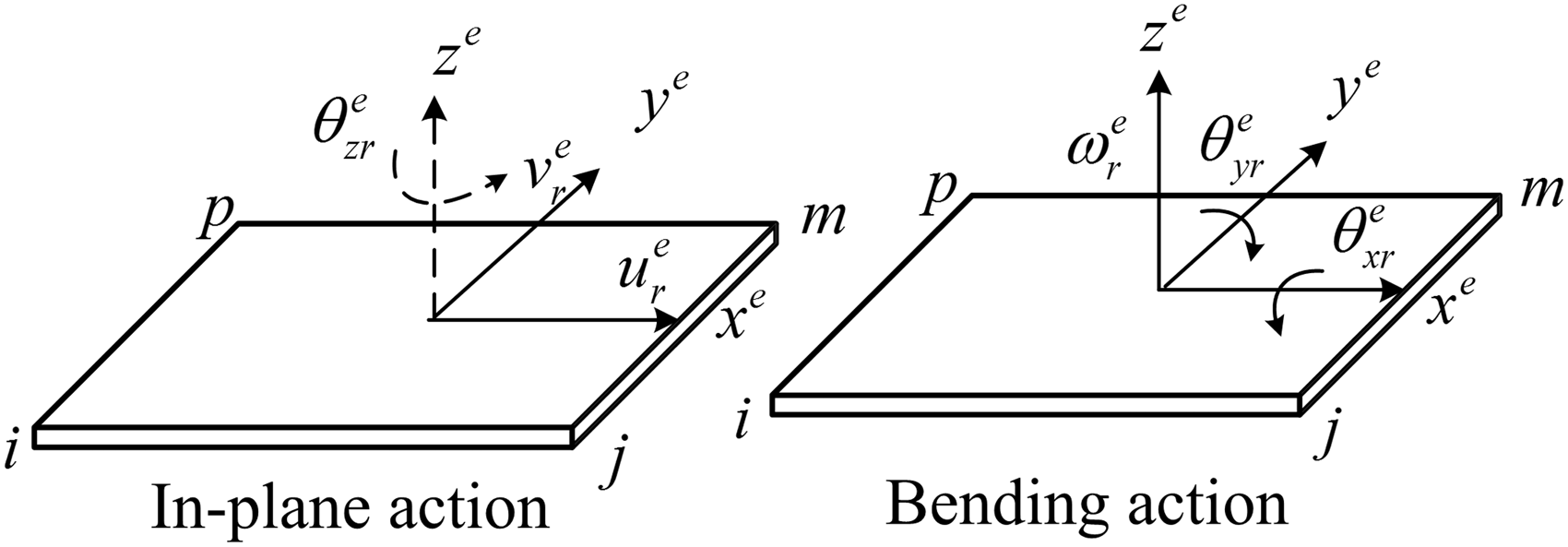
The FE method is widely applied in the analysis of complex structures since the analytical solution of that is difficult to acquire. FE methods approximately model a continuous structure by dividing it into elements. To model a shell structure, the shell can be considered as an assembly of flat shell elements (Figure 1) or as a special case of three-dimensional analysis (called degenerated shell element). The flat shell element is extremely suitable for the analysis of thin shell structures by neglecting the transverse deformation while the degenerated shell element is able to model thick structures. Since much structure in mechanical engineering can be viewed as thin structure, the flat shell element is widely applied in practice (also benefiting from its simplicity). The flat shell element assumes that the in-plane deformation and the bending deformation are independent of each other. So the deformations and stresses of the element can be viewed as a superposition of an in-plane action and bending action (shown in Figure 2).

Figure 1.

Shell represented by polygonal flat element.

Figure 2.

In-plane action and bending action of a flat plate (element e).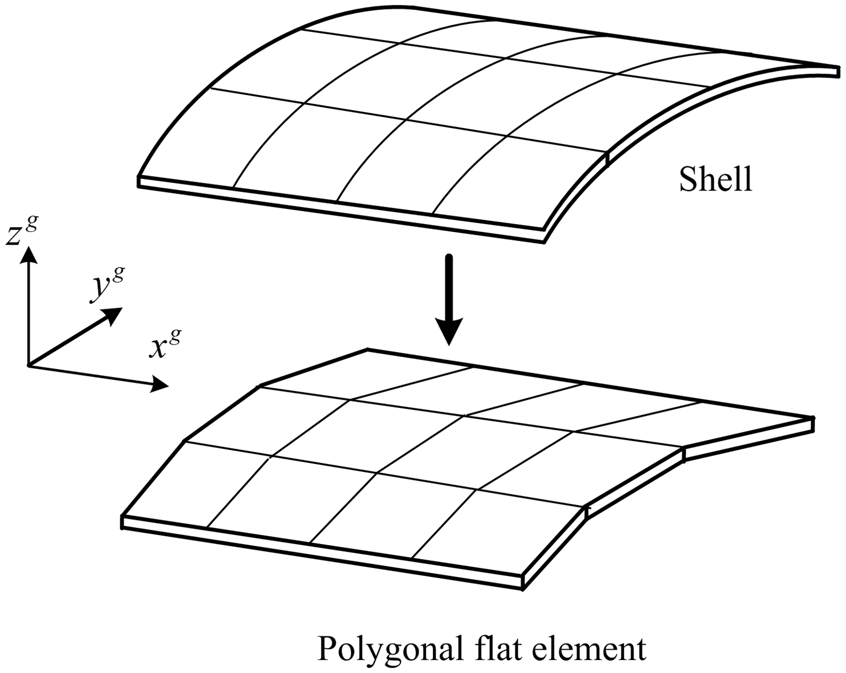

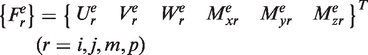
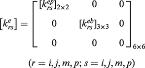
Considering a quadrature boundary shell structure, it can be modeled using a rectangle element. The global coordinates are defined as $x g y g z g$ (Figure 1) and the local coordinates of element e are defined as $x e y e z e$ (Figure 2), where g denotes global and $e = 1, 2 \dots M$ denotes the numbering of all elements. Each element has four nodes called $i, j, m, p$ and $r = 1, 2 \dots N$ denotes the numbering of all nodes. In Figure 2, there are two translations in the direction of $x e$ and $y e$ of in-plane action while there is one translation in direction of $z e$ and two rotations about $x e$ and $y e$ of bending action.

Considering the in-plane action of element e shown in Figure 2, the displacement vector and force vector of node r and their relations are

{δ r ep} = {u r e v r e} T (r = i, j, m, p)

(1)

{F r ep} = {U r e V r e} T (r = i, j, m, p)

(2)

{F r ep} = [k rs ep] {δ s ep} (r = i, j, m, p; s = i, j, m, p)

(3)

where

{δ r ep}

and

{F r ep}

denote the displacement and force vectors and the superscript p stands for in-plane;

u r e

and

U r e

are the translation and force in direction of

x e

axis while

v r e

and

V r e

are that in direction of

y e

axis;

[k rs ep]

denotes the stiffness matrix of element e of in-plane action.

Similarly, consider the bending action of element e, the displacement vector and force vector of node r and their relations are

{δ r eb} = {ω r e θ xr e θ yr e} T (r = i, j, m, p)

(4)

{F r eb} = {W r e M xr e M xr e} T (r = i, j, m, p)

(5)

{F r eb} = [k rs eb] {δ s eb} (r = i, j, m, p; s = i, j, m, p)

(6)

where

{δ r eb}

and

{F r eb}

are the displacement and force vectors and the superscript b stands for bending;

ω r e

and

W r e

are the translation and force in direction of

z e

axis,

θ xr e

and

M xr e

are the rotation and moment about

x e

axis,

θ xr e

and

M xr e

are that about

y e

axis;

[k rs eb]

denotes the stiffness matrix of element e of bending action.

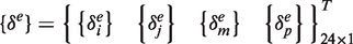
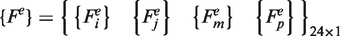
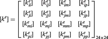
Combine the in-plane action and the bending action together:

{δ r e} = {u r e v r e ω r e θ xr e θ yr e θ zr e} T (r = i, j, m, p)

(7)

{F r e} = {U r e V r e W r e M xr e M yr e M zr e} T (r = i, j, m, p)

(8)

{F r e} = [k rs e] {δ s e} (r = i, j, m, p; s = i, j, m, p)

(9)

where

θ zr e

and

M zr e

are the rotation and moment about

z e

axis. They are useless for the element in local coordinates, but are added here to ensure the easier transformation from local to global coordinates. Connecting each node of element e to get the full displacement and force vectors:

{δ e} = {{δ i e} {δ j e} {δ m e} {δ p e}} 24 \times 1 T

(10)

{F e} = {{F i e} {F j e} {F m e} {F p e}} 24 \times 1

(11)

Since the in-plane action and bending action are independent, the combined stiffness matrix of node r of element e is

[k rs e] = [[k rs ep] 2 \times 2 000 [k rs eb] 3 \times 3 0000] 6 \times 6 (r = i, j, m, p; s = i, j, m, p)

(12)

Considering all the four nodes, the stiffness matrix of the element e is obtained:

[k e] = [[k ii e] [k ij e] [k im e] [k ip e] [k ji e] [k jj e] [k jm e] [k jp e] [k mi e] [k mj e] [k mm e] [k mp e] [k pi e] [k pj e] [k pm e] [k pp e]] 24 \times 24

(13)

The stiffness matrix

[k e]

is actually in local coordinates and the matrix element consists of the stiffness of in-plane and bending actions. Reference books can be consulted (Cook et al., 1989; Zienkiewicz and Taylor, 2005) to find details.

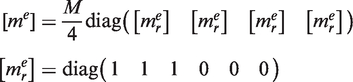
The mass matrix of the element can be obtained using lumped mass matrix theory by considering each nodes share the same mass of an element and ignoring the rotation mass. It is

[m e] = \frac{M}{4} diag ([m r e] [m r e] [m r e] [m r e]) [m r e] = diag (111000)

(14)

where M is the mass of the element e and the mass matrix

[m e]

is also in local coordinates.

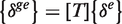
Now the element matrices in local coordinates must be transferred into global coordinates, using the coordinate transformation matrix T, which is defined as

[T] = diag ([λ] [λ] [λ] [λ]) [λ] = diag ([λ'] [λ']) [λ'] = [λ x e x g λ x e y g λ x e z g λ y e x g λ y e y g λ z e z g λ z e x g λ z e y g λ z e z g]

(15)

where

λ x e x g

is the direction cosine of

x e

axis and

x g

, others are deduced analogously (Zienkiewicz and Taylor, 2005).

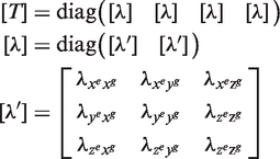
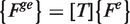
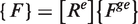
So the displacement vector, force vector, stiffness matrix and mass matrices of element e in global coordinates are

{δ ge} = [T] {δ e}

(16)

{F ge} = [T] {F e}

(17)

[k ge] = [T] T [k e] [T]

(18)

[m ge] = [T] T [m e] [T]

(19)

Assemble all the elements vectors and matrices together and there are the assembled displacement and force vectors as well as the assembled stiffness and mass matrices:

{U} = [R e] {δ ge}

(20)

{F} = [R e] {F ge}

(21)

[M] = \sum_{e = 1}^{M} [R e] T [m ge] [R e]

(22)

[K] = \sum_{e = 1}^{M} [R e] T [k ge] [R e]

(23)

where

{U}

and

{F}

are (6 N × 1) assembled displacement and force vectors; [M] and [K] are (6 N × 6 N) assembled stiffness and mass matrices;

[R e]

is a (6 N × 24) matrix stands for the node position of element e in global vectors (Cook et al., 1989).

1.2. Lumped parameter model of an electrodynamic actuator

Since the electrodynamic actuator has a wide frequency range and loading range, it is the most widely used actuator especially in the excitation of medium-large structures. Moreover, it is easy to control and can produce a better complex waveform and be extremely favored by the laboratory.

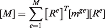
Figure 3 shows the simplified lumped parameter model of the electrodynamic actuator. k_a is the equivalent stiffness of the actuator, c_a is the equivalent damping of the actuator and m_a is the mass of the movable part of the actuator. f_e is the electromagnetic force and f_s is the reactive force of the controlled structure. f_e is decided by

f e = BIL

(24)

where I is the current of coil. B is the magnetic strength. L is the length of wire that cut the magnetic curves. For a constant current amplifier, there is

I = β V o

(25)

where β denotes the current amplification coefficient and V_o denotes the output voltage of the computer. Consider

BL

as a constant, there is

f e = α β V o

(26)

where

\binom{α Δ}{= BL}

, so the mathematical model of the actuator is

m a \overset{··}{x} a + c a \overset{\cdot}{x} a + k a x a = f e - f s = α β V o - f s

(27)

Figure 3.

Mechanical model of an electrodynamic actuator.

2. Formulation of dynamic response of the coupled model

2.1. Coupling of structure and actuators

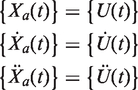
Since the shell structure is a complex distributed parameter system, it can be dispersed in the space dimension to get the following semi-discretization matrix differential equation:

[M] {\overset{··}{U} (t)} + [C] {\overset{\cdot}{U} (t)} + [K] {U (t)} = {F s (t)}

(28)

where

{U (t)}

is the global displacement vector defined by equation (20) and is now a time-dependent function in the dynamic problem;

{\overset{\cdot}{U} (t)}

and

{\overset{··}{U} (t)}

denote the global velocity and acceleration vectors. They are defined by the first and second derivative of

{U (t)}

with respect to time; [M] and [K] are the assembled mass and stiffness matrix defined by equations (22) and (23). [C] is the damping matrix and defined by a popular spectral damping scheme called Rayleigh (or proportional) damping. It is to form the damping matrix as a linear combination of the stiffness and mass matrices, that is

[C] = a [M] + b [K]

(29)

where a and b are called stiffness and mass proportional damping constants, respectively.

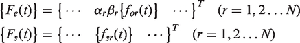
Assume that the central axis of the sell is in z direction. For an actuator connected with the structure at node r (named actuator r), the direction of the force component is along x and y axis (assume force component along z and moments about xyz are zero). So the mechanical model of such an actuator can be rewritten as

[m r] {\overset{··}{x} r (t)} + [c r] {\overset{\cdot}{x} r (t)} + [k r] {x r (t)} = α r β r {V or (t)} - {f sr (t)} (r = 1, 2 \dots N)

(30)

where the parameter matrices of actuator are

[m r] = diag (γ 1 m r γ 2 m r 0000) [c r] = diag (γ 1 c r γ 2 c r 0000) [k r] = diag (γ 1 k r γ 2 k r 0000)

(31)

and the force vectors of actuator are

{V or (t)} = {γ 1 V or γ 2 V or 0000} T {f sr (t)} = {γ 1 f sr γ 2 f sr 0000} T

(32)

In the equations (30)–(32), m_r, c_r and k_r denote the movable mass, the equivalent damping and equivalent stiffness of actuator r, respectively;

V or

denotes the output voltage from the computer for actuator r and

f sr

denotes the reactive force to actuator r;

γ 1

and

γ 2

are the distribution coefficients.

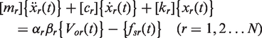
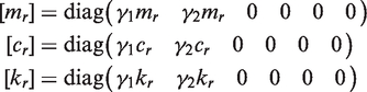
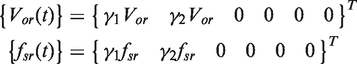
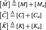
Consider multiple actuators (N actuators) are connected to the structure, the added mass, added damping and added stiffness matrices are defined as

[M a] = diag ([m 1] \dots [m r] \dots [m N]) [C a] = diag ([c 1] \dots [c r] \dots [c N]) [K a] = diag ([k 1] \dots [k r] \dots [k N])

(33)

And the force vectors of the actuators are defined as

{F e (t)} = {\dots α r β r {f or (t)} \dots} T (r = 1, 2 \dots N) {F s (t)} = {\dots {f sr (t)} \dots} T (r = 1, 2 \dots N)

(34)

where if there are no actuators connected to certain nodes, matrices of equation (31) and vectors of equation (32) can be set as zeros.

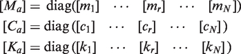
Assemble all the actuators equation together to get:

[M a] {\overset{\cdot\cdot}{X} a (t)} + [C a] {\overset{\cdot}{X} a (t)} + [K a] {X a (t)} = {F e (t)} - {F s (t)}

(35)

The displacement, velocity and acceleration of actuators are equal to that of the structure at the connection points, i.e.

{X a (t)} = {U (t)} {\overset{\cdot}{X} a (t)} = {\overset{\cdot}{U} (t)} {\overset{··}{X} a (t)} = {\overset{··}{U} (t)}

(36)

Deducing from equation (28), equation (35) and equation (36), the vibration equation of structure considering the influence of actuators is

[\bar{M}] {\overset{··}{U} (t)} + [\bar{C}] {\overset{\cdot}{U} (t)} + [\bar{K}] {U (t)} = {F e (t)}

(37)

where

[\bar{M}] \overset{Δ}{=} [M] + [M a] [\bar{C}] \overset{Δ}{=} [C] + [C a] [\bar{K}] \overset{Δ}{=} [K] + [K a]

(38)

2.2. Dynamic response of a damped second-order system

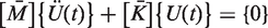
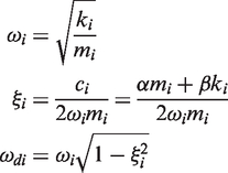
To analyze the forced vibration of the system, the free vibration of it should be solved first to get the nature frequencies and modal shapes. If no damping and forcing terms exist in the dynamic problem of equation (37), it reduces to

[\bar{M}] {\overset{··}{U} (t)} + [\bar{K}] {U (t)} = {0}

(39)

A general solution of such an equation can be written as

{Φ} \sin (ω t + φ)

. Substitute it back to equation (39), it was found that ω can be determined from

([\bar{K}] - ω 2 {\bar{M}}) {Φ} = {0}

(40)

where

[K] - ω 2 [M]

denotes the eigenmatrix, ω denotes the eigenvalue and {Φ} denotes the eigenvector. For non-zero solutions, the determinant of the eigenmatrix must be zero, i.e.

det ([\bar{K}] - ω 2 [\bar{M}]) = 0

(41)

[\bar{K}]

and

[\bar{M}]

are symmetric positive definite matrices, equation (41) will in general give n positive value of ω². Gather all the values of ω into a vector

{Ω} = {ω 1 ω 2 \dots ω n}

by ascending order, where

ω i (i = 1, 2 \dots n)

denotes the ith eigenvalue (i.e. the ith nature frequency).

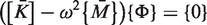
The corresponding eigenvector is ${Φ i} (i = 1, 2 \dots n)$ indicating the ith modal shape. They are also gathered and sorted in the same order as $ω i$ into a matrix $[Φ] = [{Φ 1} {Φ 2} \dots {Φ n}]$ called the modal matrix. By pre-multiplying each term of equation (37) $[Φ] T$ , the equation is decoupled, i.e.

[M p] {\overset{··}{η} (t)} + [C p] {\overset{\cdot}{η} (t)} + [K p] {η (t)} = {Q (t)}

(42)

where

{η (t)}

{\overset{\cdot}{η} (t)}

{\overset{··}{η} (t)}

and

{Q (t)}

denote the modal displacement, velocity, acceleration and force vectors, respectively.

[M p]

[C p]

and

[K p]

denote the decoupled (diagonal) mass, damping and stiffness matrix. Each terms of equation (42) are defined as follows

η (t) = [Φ] - 1 {U (t)} [M p] = [Φ] T [M] [Φ] [K p] = [Φ] T [K] [Φ] [C p] = [Φ] T [C] [Φ] = a [M p] + b [K p] {Q (t)} = [Φ] T {F e (t)}

(43)

Consider the ith equation of the decoupled matrix differential equation (equation (42)):

m i \overset{··}{η} i (t) + c i \overset{\cdot}{η} i (t) + k i η i (t) = q i (t) (i = 1, 2 \dots 6 N)

(44)

where m_i, c_i and k_i denote the diagonal elements of

[M p]

[C p]

and

[K p]

, q_i and

η i (t)

denote the elements of

{Q (t)}

and

{η (t)}

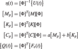
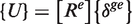
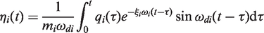
For an arbitrary input, the zero initial conditions solution of equation (44) is

η i (t) = \frac{1}{m i ω di} \int 0 t q i (τ) e - ξ i ω i (t - τ) \sin ω di (t - τ) d τ

(45)

where

ω i

denotes the ith natural frequency,

ξ i

denotes the ith modal damping and

ω di

denotes the ith damping frequency. They are decided by

ω i = \sqrt{\frac{k i}{m i}} ξ i = \frac{c i}{2 ω i m i} = \frac{α m i + β k i}{2 ω i m i} ω di = ω i \sqrt{1 - ξ i 2}

(46)

From equations (42)–(46), the modal displacement vector

{η (t)}

is obtained. So the displacement response in the physical coordinate is

{U (t)} = [Φ] {η (t)}

(47)

where

[Φ]

is the modal matrix.

3. Feature analysis of the coupled model

3.1. Numerical implementation of the clamped shell

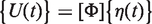
In the following, a clamped-free shell as illustrated in Figure 4(a) is considered. The global coordinate are erected in Figure 4(a) and the size and engineering data are listed in Table 1.

Figure 4.

Modeling of a clamped-free shell. (a) sketch of a clamped-free shell, (b) discretization of the shell.

Table 1.

Parameters of the active control system.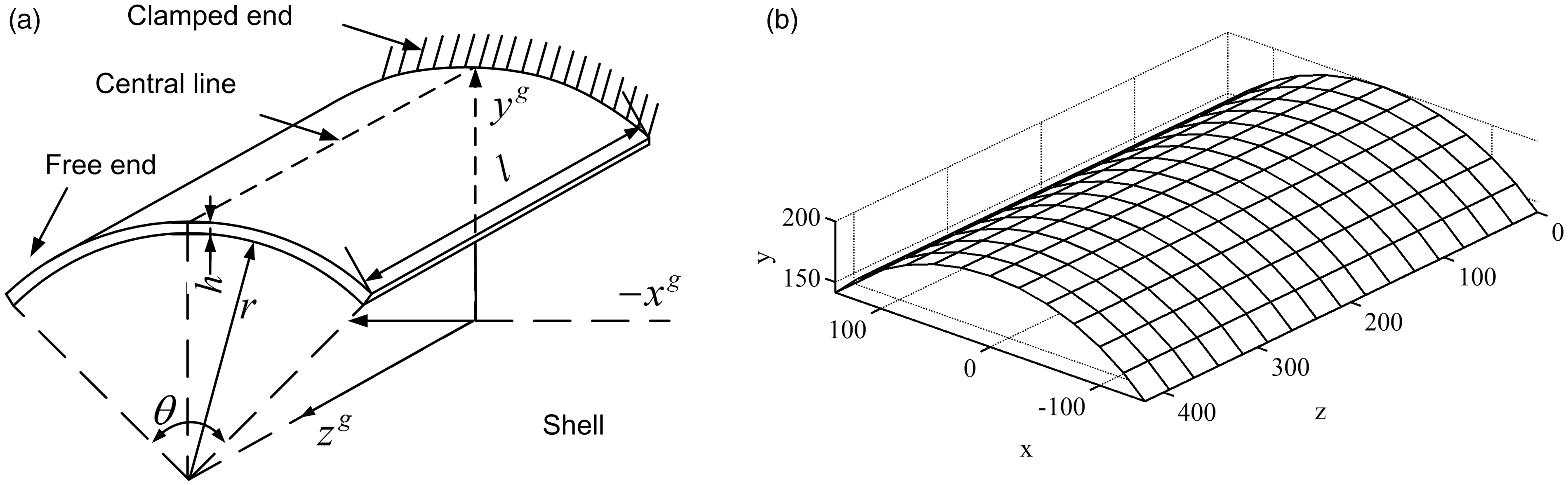

Size	Symbol	Value	Engineering data	Symbol	Value
Length (m)	l	0.42	Elastic modulus (Pa)	E	2 × 10¹¹
Radius (m)	r	0.2	Poisson’s ratio	ɛ	0.3
Thickness (m)	h	0.005	Density (kg/m³)	ρ	7.85 × 10³
Central angle	θ	90^o	Modal damping ratio	ξ	0.01

The whole shell is divided into 12 × 16 rectangle elements (Figure 4(b)). Each element has four nodes and there are 221 nodes in total and each node has six degrees-of-freedom (d.f.).

The clamped end implies that all the 13 nodes in the circumferential line where z = 0 is constrained in all d.f., so the total d.f. of the shell is 13 × 16 × 6 = 1248. Moreover, the size of mass, damping and stiffness matrix are the square of the total d.f. Since the amount of calculation of 1248 × 1248 matrices is a little bit large in the control loop, the translation d.f. as the main d.f. of the system are considered, so the calculation amount is reduced to 624 × 624. The geometry modeling process is to solve equation (1) to equation (23) to obtain the global mass, damping and stiffness matrices. The model was calculated and illustrated using MATLAB.

3.2. Optimal configuration of sensors and actuators

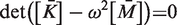
In the following part, modal analysis and harmonic response analysis are applied to discuss the vibration characteristics of the shell and finally to decide where to mount actuators and sensors. The aim of modal analysis was to recognize the modal parameters of the clamped shell structure. Solving equations (37)–(43) and ignoring the influence of the actuators (i.e. let the matrices $[M a]$ , $[C a]$ and $[K a]$ be zero), the nature frequency vector ${Ω}$ and modal matrix $[Φ]$ are obtained. Since the total d.f. of the system are 624, there are 624 nature frequencies and 624 modal shapes in theory. But a large amount of higher order nature frequencies and modal shapes have less influence on the characteristic of the structure. Moreover, the higher order characteristic is inaccurate by the FE method. Therefore, only the first few modes and nature frequencies have been studied.

Figure 5 shows the first four modes of the clamped-free shell. The displacement of each mode is added to the original coordinates (35 × magnification). Figure 5(a) shows the first mode (114.06 Hz) of the shell. The deformation direction of the left free end and right free end are opposite, which means there is a nodal line in the middle of the shell. The intersection line of the deformed surface (the colored surface) and the undeformed surface (the mesh surface) is the nodal line. Figure 5(b) shows the second mode (219.17 Hz) of the shell. The deformation directions of all the nodes are the same, just like the first mode of a clamped-free plate. Figure 5(c) shows the third mode (345.26 Hz), which has the second-order bending in the direction of z axis. Lastly, the fourth mode (482.1 Hz) shown in Figure 5(d) has the second-order bending in both in z axis and circumferential directions.

Judging from the mode shapes, the maximum displacement may happen at the free end and there may be a nodal line in the middle of the shell which must be avoided when mounting actuators and sensors. To confirm the judgment, the harmonic response analysis has been conducted. Four typical excitation positions are chosen and they are located at the right free end, the left free end, the right middle edge and on the central line as shown in Figure 6.

For all the four cases, the excitation input is 10 Hz unit sinusoidal force in a radial direction. From the linear system theory, the response of each node is 10 Hz sinusoidal wave with different amplitudes and initial phases. So the vibration deformations of each node in Figure 6 are decided by the amplitude of the sinusoidal responses and the directions of that are decided by the initial phase of the responses.

Figure 5.

First four mode shapes of the clamped-free shell. (a) Mode 1 (114.06 Hz), (b) mode 2 (219.17 Hz), (c) mode 3 (345.26 Hz), and (d) mode 4 (482.10 Hz).

Figure 6.

Harmonic responses at different excitation points. (a) Case 1: the right-free-end excitation, (b) case 2: the left free-end excitation, (c) case 3: the right-middle-edge excitation, (d) case 4: the modal line excitation.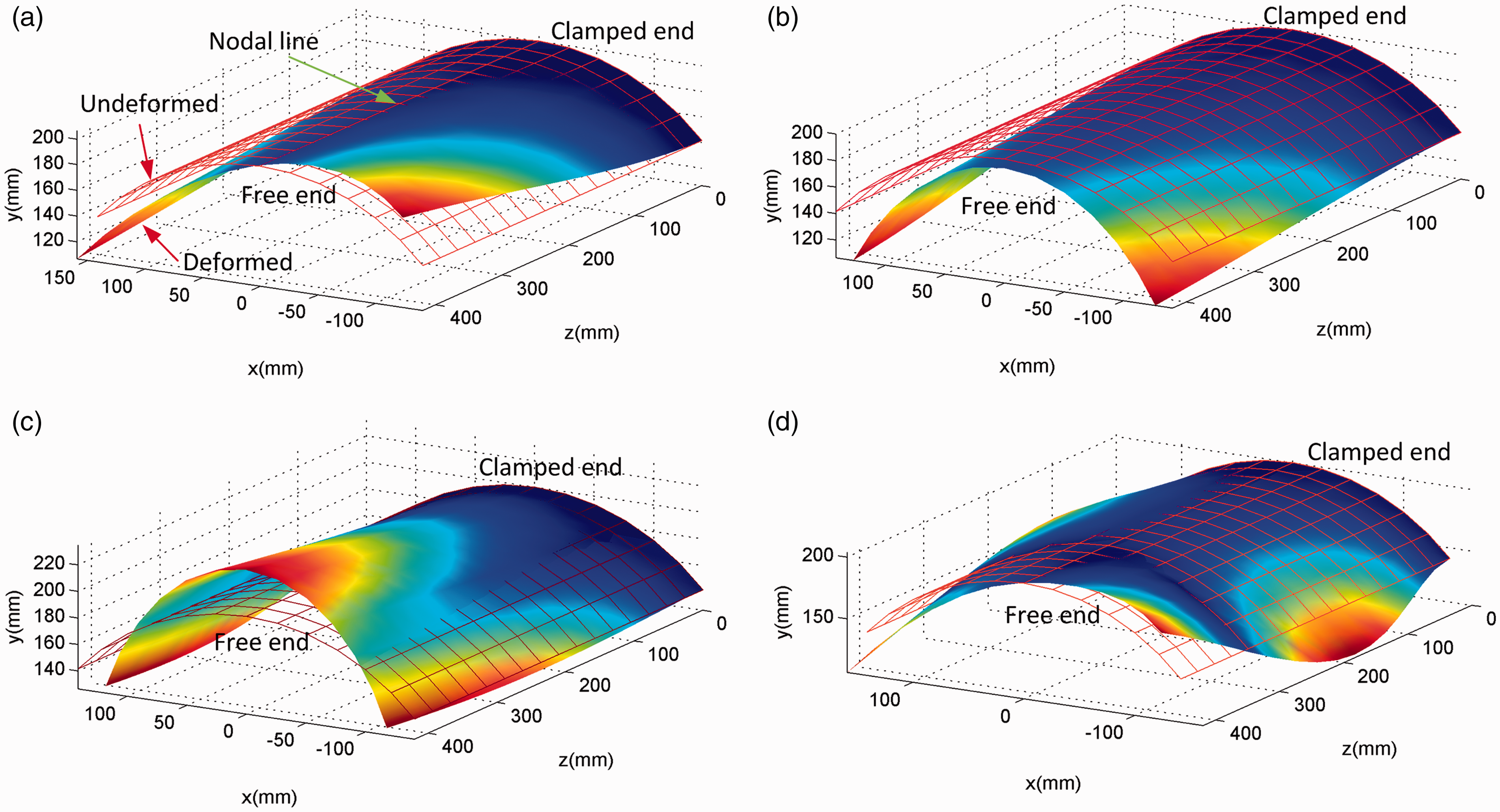

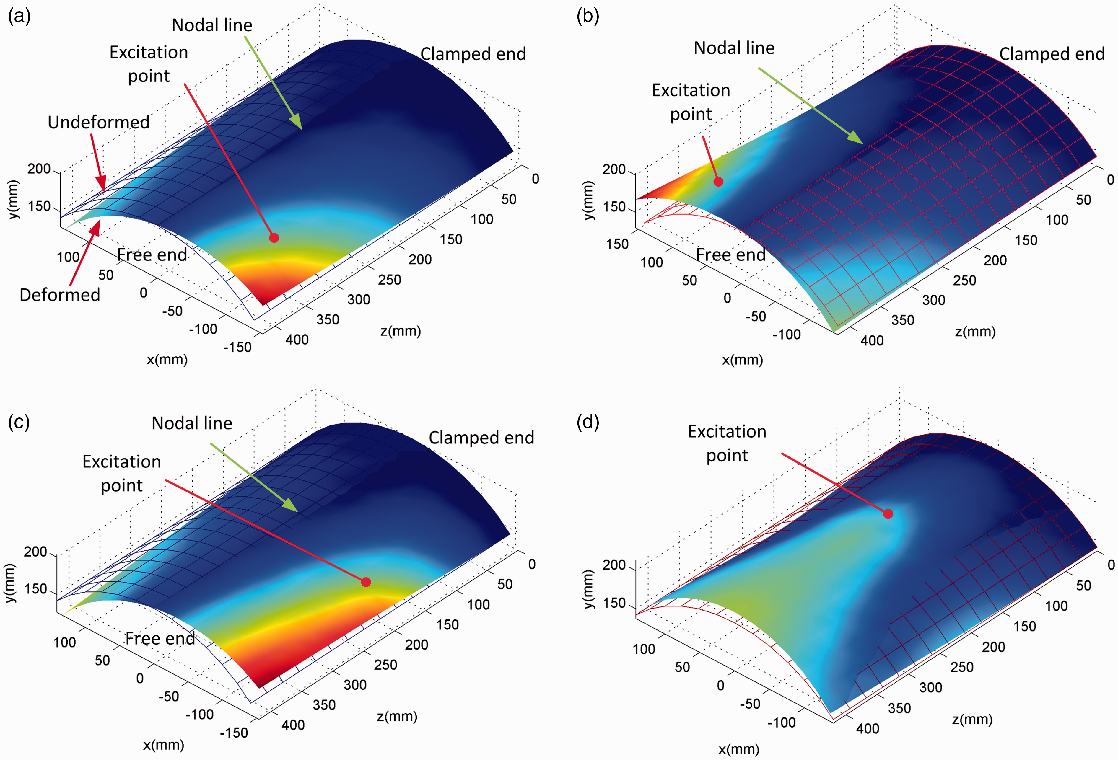
The maximum deformation of each case is 2.72 mm, 2.72 mm, 0.89 mm and 0.11 mm, respectively.

Figure 6(a) and (b) shown that the structure is symmetry and excitation on one side will lead the same direction response on the same side and the opposite direction response on the opposite side. So there is a nodal line in the middle of the shell in actual response.

Figure 6(a) and (c) show that excitations on the same side lead to same direction’s deformation. Moreover, the closer the excitation positions are to the clamped end, the smaller the responses are.

Figure 6(d) shows that the nodal line excitation leads to the same deformation direction just like mode 2 in Figure 5(b). If the excitation is located on the nodal line the first mode will not be motivated where the second mode will be dominant. But it is notable that the response case4 is much smaller than that of the other cases.

Therefore the conclusion is arrived at: it is better to avoid the nodal line (i.e. the central line on surface) and give priority to the free end or the edges when mounting the actuators and sensors.

3.3. Influence of the actuators

Following the principle summarized in 3.2, three actuators have been mounted to the shell. They are connected to the left and right free end and the right middle edge where the deformation is remarkable (Figure 7). Assume that the excitations are loaded in a radial direction, so they can be divided into x component and y component. The distribution coefficients (defined in equations (31) and (32)) of each component are shown in Table 2 and they are related to the amplitude and direction of the forces. Assuming the angle between y axis and the force is θ, the distribution coefficient of y axis is $\sin θ$ and that of z axis is $\cos θ$ .

The sensors are mounted in the same position with actuators. The movable mass, equivalent damping and equivalent stiffness of actuators affect the characteristic of the structure. The parameters of the actuators are shown in Table 3. They are referenced from a mini-electrodynamic actuator from a Chinese supplier.

“The influence of the actuators” means that the influence of the added matrices is taken into account when solving the eigenvalue problem of equation (39). From the analysis before, equations (30)–(33) decide the added matrices. The nature frequencies of the shell considering the coupling effect of actuators are shown in Table 4. It can be seen that the mount of actuators diminish the natural frequency of the structure and the influence is extremely large to the second and sixth order frequencies. The added mass pulls down the natural frequencies and the added stiffness pulls them up. Since stiffness of the steel shell is much greater than that of the leaf spring of the actuators so the pull down effect is more remarkable.

Figure 7.

Mount of actuators (radial direction).

Table 2.

Distribution coefficient of each excitation point.

Excitation position	Angle between normal direction and + x axis (degree)	Distribution coefficient of
Excitation position	Angle between normal direction and + x axis (degree)	X component $γ 1$	Y component $γ 2$	Z component
S	127.5	−0.609	0.793	0
P1	127.5	−0.609	0.793	0
P2	52.5	0.609	0.793	0

Table 3.

Parameters of actuators.

Property	Symbol	Value
Movable mass of actuator (kg)	m_a	0.03
Equivalent damping of actuator (Ns/m)	c_a	5.5
Equivalent stiffness of actuator (N/m)	k_a	1000

Table 4.

Influence on natural frequency.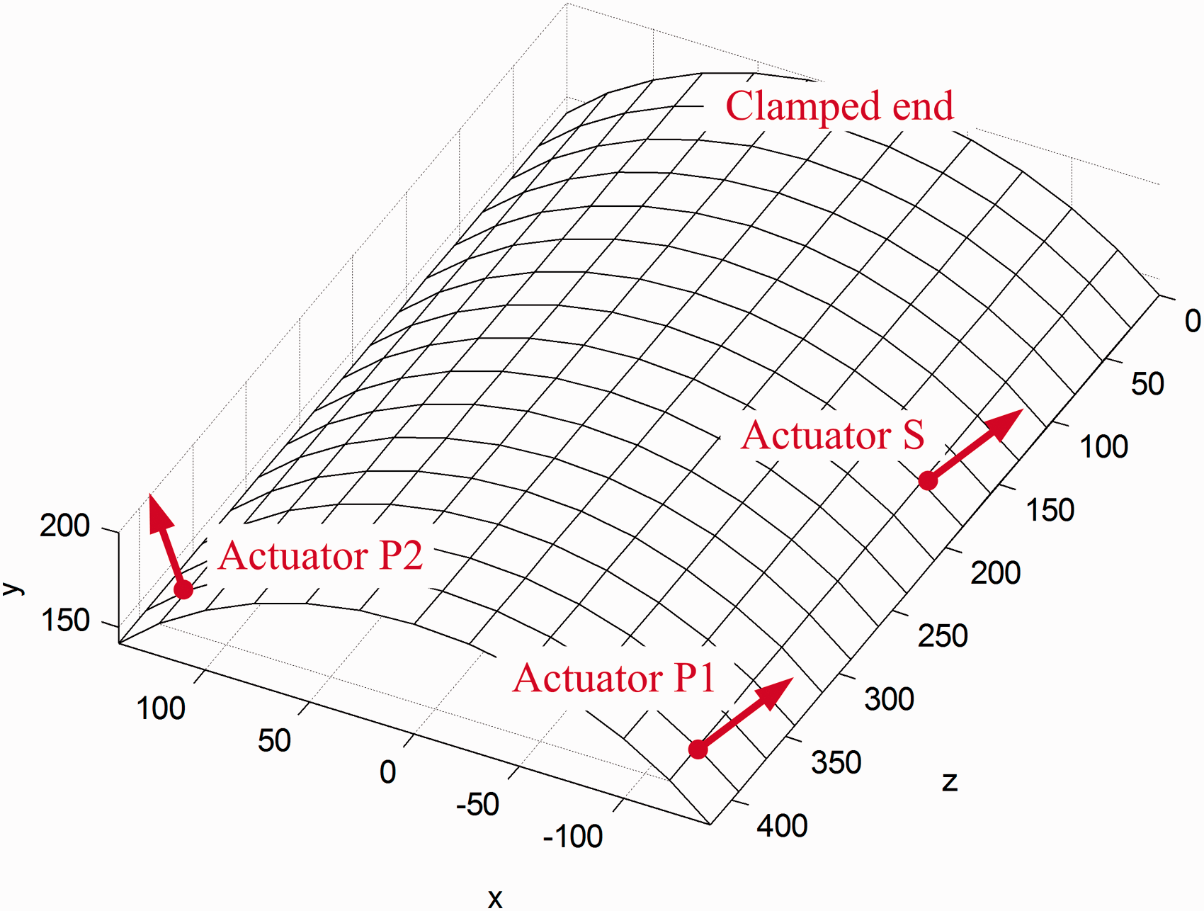

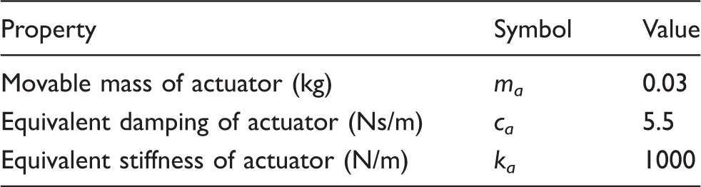
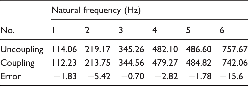
	Natural frequency (Hz)
No.	1	2	3	4	5	6
Uncoupling	114.06	219.17	345.26	482.10	486.60	757.67
Coupling	112.23	213.75	344.56	479.27	484.82	742.06
Error	−1.83	−5.42	−0.70	−2.82	−1.78	−15.6

Figure 8 shows frequency response functions (FRFs) from actuator S to actuators P1 and P2, which reveal the influence of the actuators from another angle. From the figure, it can be found that except for the decrease of natural frequencies (mainly affected by the added mass and stiffness), the resonance peak becomes smoother. This was mainly influenced by the added damping. Then, the FRFs of y direction are larger than that of x direction which means the response in y direction is more remarkable. Moreover, the phase frequency diagram gives much information. When the excitation frequency is lower than the first natural frequency, the phase lag is about zero. When the excitation frequency is greater than the first natural frequency, the phase lag is significant, but never exceeds 180 degree (Figure 8(a)). The direction of response of the opposite side of the shell is opposite to the excitation. It can be view as a 180 degree phase lag in low frequency (Figure 8(b)).

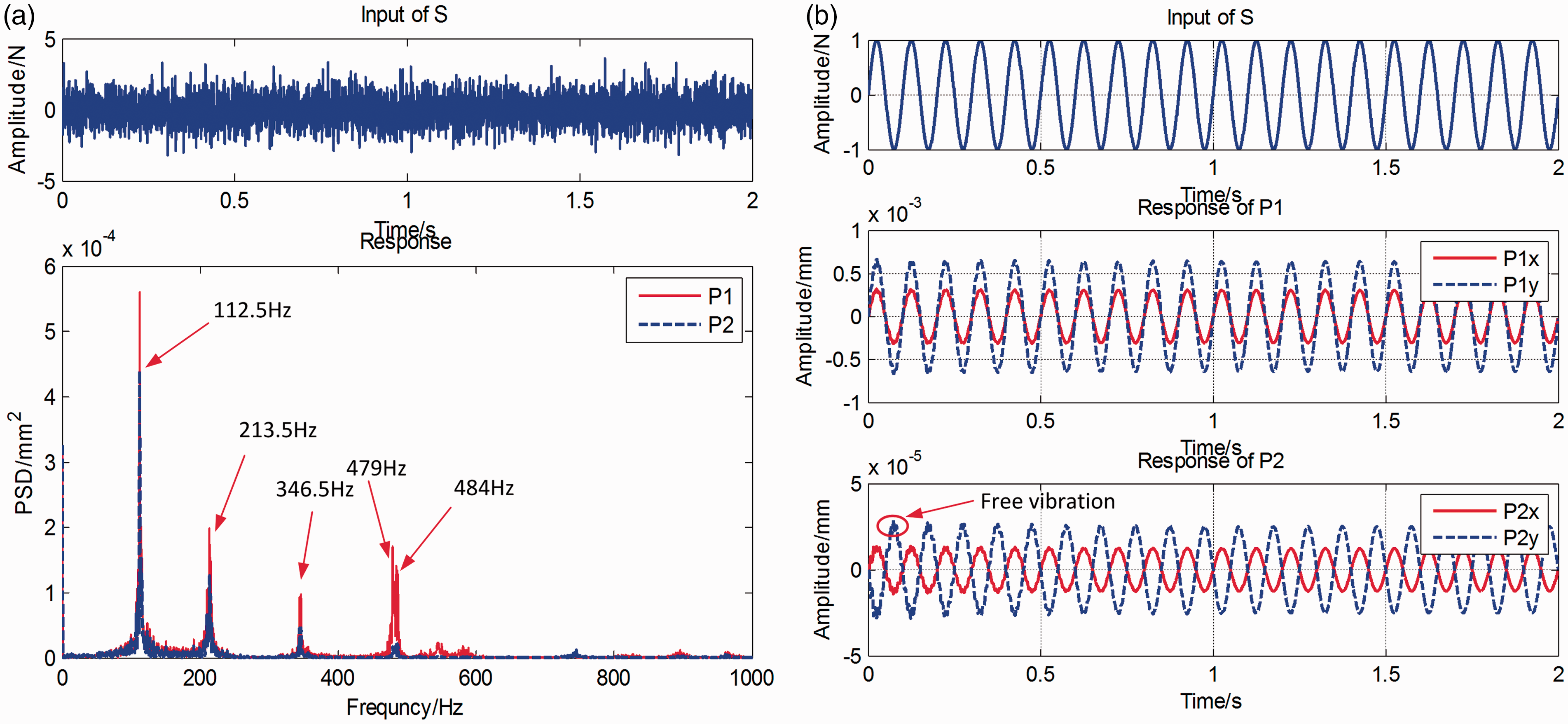
The coupled model is determined and the time series dynamic response of the system haven been investigated. Random and sinusoidal inputs are given by actuator S and the response of P1 and P2 are considered. It can be seen from Figure 9(a) that the random response accurately identifies the first five resonant frequencies of the coupled model. The frequencies have slight errors to the value in Table 1 which can be reduced by adding the number of tests and then averaging. The sinusoidal response is shown in Figure 9(b), where the small wave of the response in the first few periods is the free vibration of the structure. It accurately showed the influence of damping, the damping suppresses free vibration of the structure and the responses quickly change to forced vibration (the smooth sine wave).

Figure 8.

Frequency response functions of the disturbance source to second sources. (a) FRFs from actuator S to actuator P1, (b) FRFs from actuator S to actuator P2.

Figure 9.

Dynamic response of the coupled model. (a) Random response, (b) Sinusoidal response.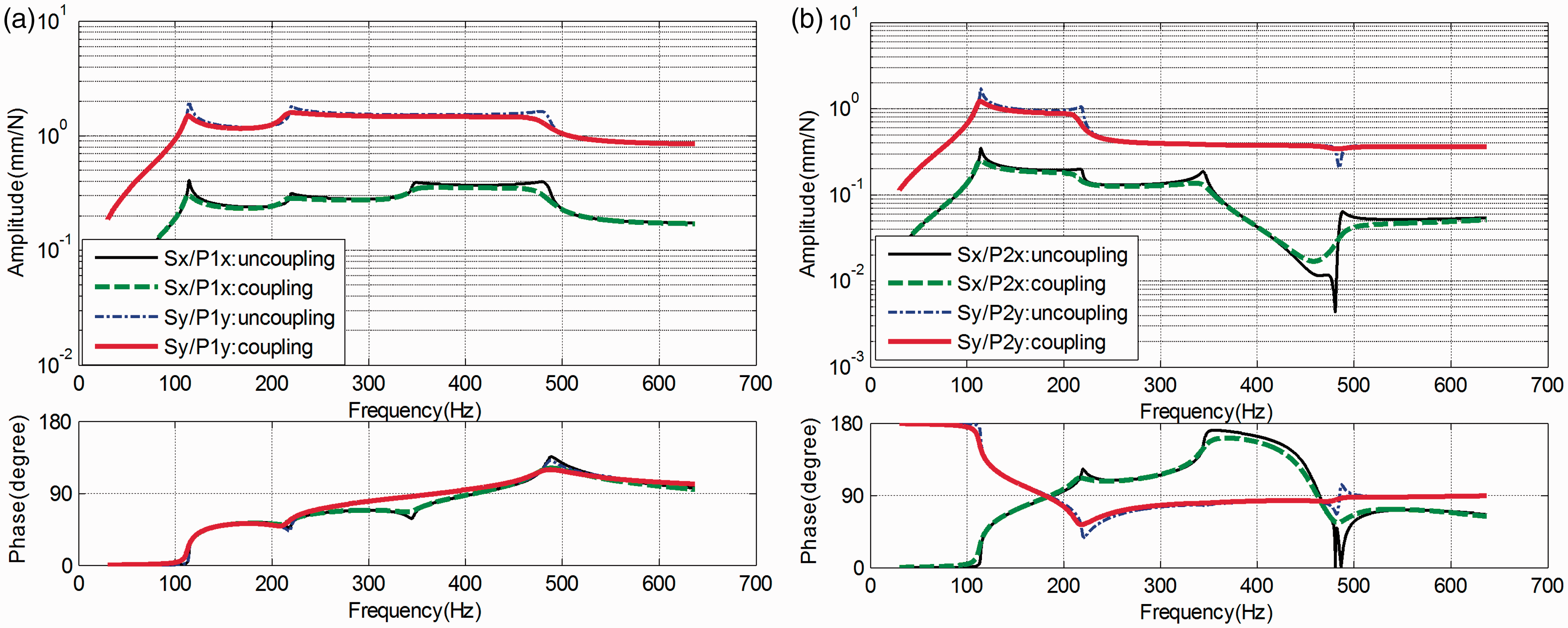

4. Active vibration control of the coupling model by filtered-reference least mean square (fxlms) algorithm

4.1. Formulation of the FXLMS algorithm

The vibration of machines is complicated, but vibration sources are usually caused by rotation machinery, which is generally a periodic signal. For this kind of disturbance the adaptive filter method is usually preferable. The filtered-reference least mean square (FXLMS) algorithm is a well-known method to solve this kind of problem. Since the reference signal is usually defined as x(t), so it is also called the FXLMS algorithm. The schematic diagram of FXLMS is shown in Figure 10. The error signal and reference signal are taken from the structure to build the algorithm and the structure receives the control excitation from actuators. H is the primary channel from source to the observation point and $S 1 + S 2$ is the secondary channel from filter to observation point.

There are two filters in the FXLMS algorithm, first one is filter S which is an identification of the secondary path of $S 1 + S 2$ and the second filter is filter W which is an adaptive filter to adjust the excitation signal $y (n)$ :

y (n) = \sum_{l = 0}^{L - 1} w l x (n - l) = {X L (n)} T {W (n)} {X L (n)} = {x (n) x (n - 1) \dots x (n - L + 1)} T {W (n)} = {w 0 w 1 \dots w L - 1} T

(48)

where L denotes the length of filter W and

x (n)

denotes the reference signal;

w i (i = 0, 1 \dots L - 1)

denotes the weight of filter W , they are changeable in the iteration.

Figure 10.

Schematic of the filtered-reference least mean square (FXLMS) algorithm.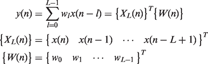

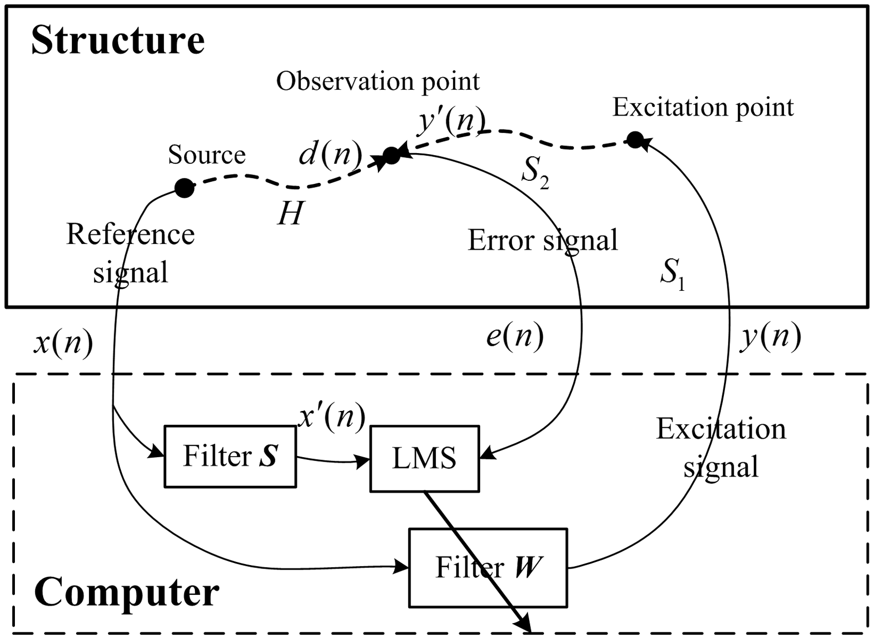
The output of filter S is used for the LMS algorithm to adjust the weight of filter W :

x' (n) = \sum_{h = 0}^{H - 1} s h x (n - h) = {X H (n)} T {S} {X H (n)} = {x (n) x (n - 1) \dots x (n - H + 1)} T {S} = {s 0 s 1 \dots s H - 1}

(49)

where H is the length of filter S and

s i (i = 0, 1 \dots H - 1)

denotes the weight of filter S . Filter S is the identification of the secondary channel and its weights are usually considered to be constant in a simple situation.

The LMS unit is to adjust the weight of filter W , it is

W (n + 1) = W (n) + 2 μ e (n) X' L (n) X' L (n) = [x' (n) x' (n - 1) \dots x' (n - L + 1)] T

(50)

where

e (n)

is the response of observation point.

Consider equation (37): the source signal and excitation signal are the inputs of the equation and the error signal is the response of the equation, so the simulation system is implemented by combining it to equations 48–50.

4.2. Control effect

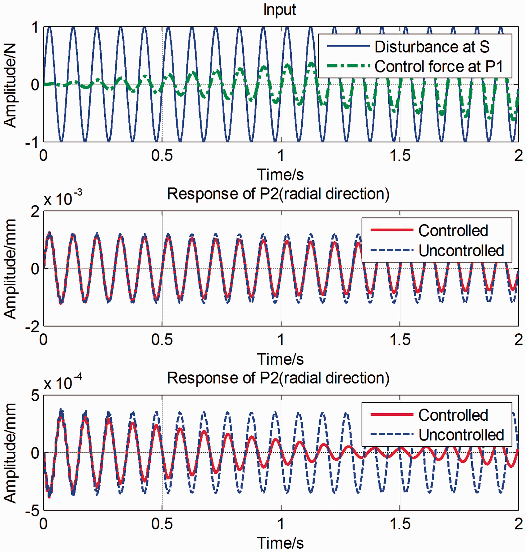
The actuator S simulates the disturbance source and the actuators P1 and P2 act as the secondary source to suppress the disturbance. Figure 11 shows the disturbance suppression by actuator P1 with the error signal taken from P1 too. The control force is inverted to the disturbance and the amplitude adjusts to a steady value. Both the response of P1 and P2 are decreased by carrying out the control. Figure 12 shows the disturbance suppression by actuator P2 with the error signal taken from P2 too. The decrease of the amplitude is slower and there is no steady point. The amplitude of P2 is reduced to minimum and then increased. Therefore it is good to apply the control at P1 where it is closer to the source.

Figure 11.

Disturbance suppression by actuator P1.

Figure 12.

Disturbance suppression by actuator P2.

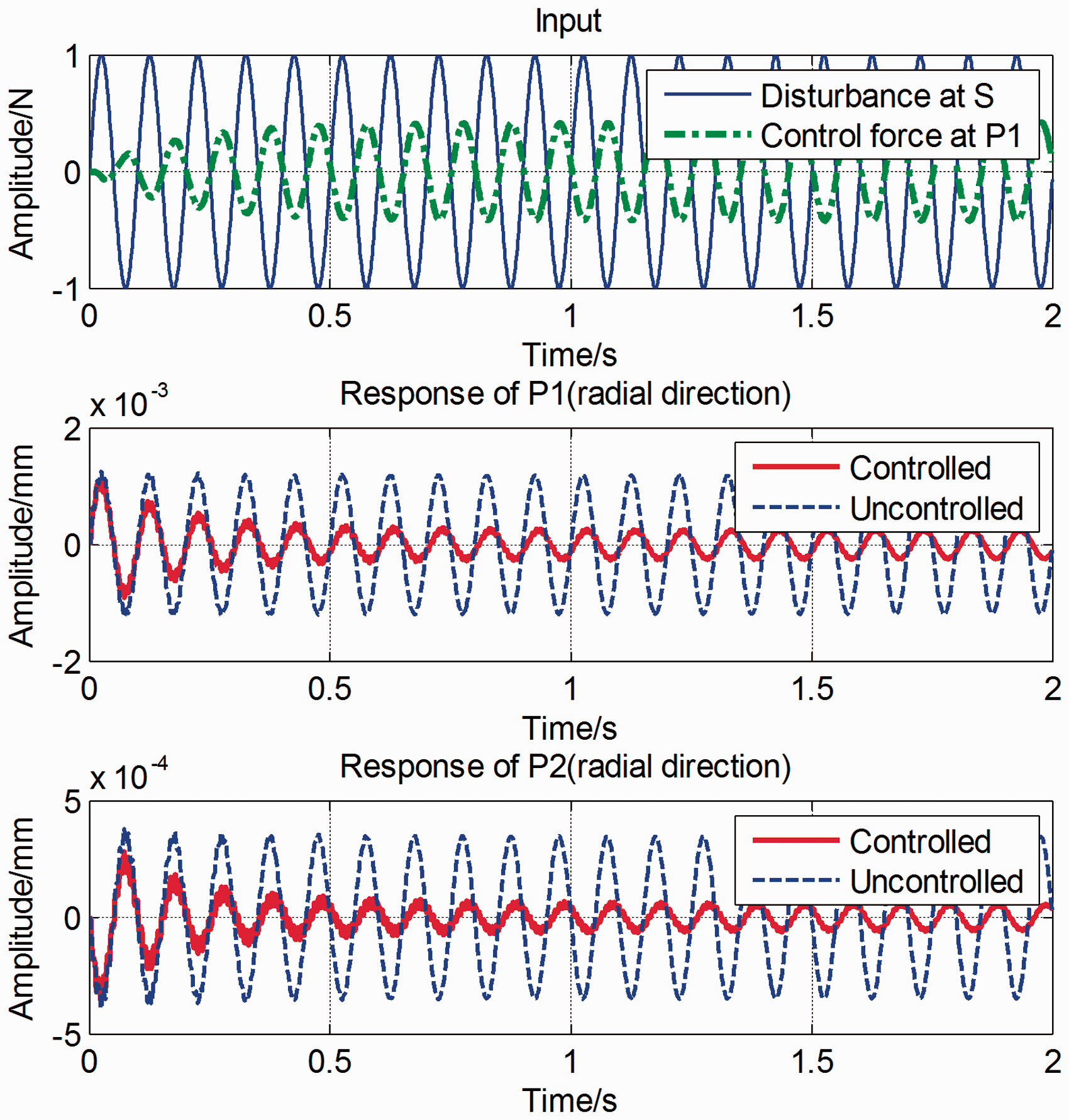
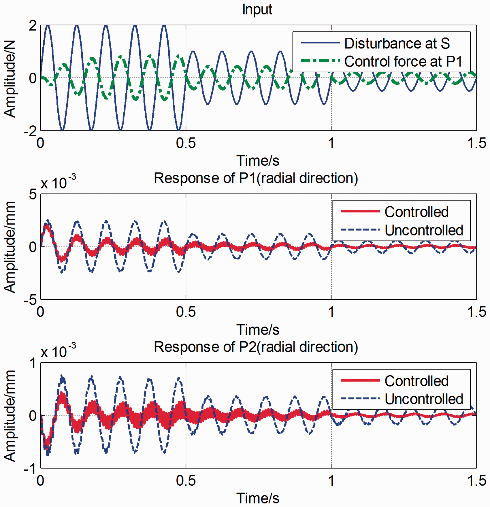
A multi-frequency disturbance has been applied and is shown in Figure 13. It can be seen that the control force is also inverse to the disturbance and the response of the P1 and P2 are suppressed. Moreover, the amplitude of the disturbance may change in a practical situation, so the varying amplitude disturbance was considered. Figure 14 applied the down jumps of the amplitude of the disturbance at 0.5 s and 1 s. The control effected shows that the algorithm can handle the amplitude-varying situation. Furthermore, it shows that the simulation system was conducted point by point in the time domain and can be easily extended to the real system.

Figure 13.

Multiple-frequency disturbance (10 Hz and 40 Hz) suppression.

Figure 14.

Amplitude-varying disturbance suppression.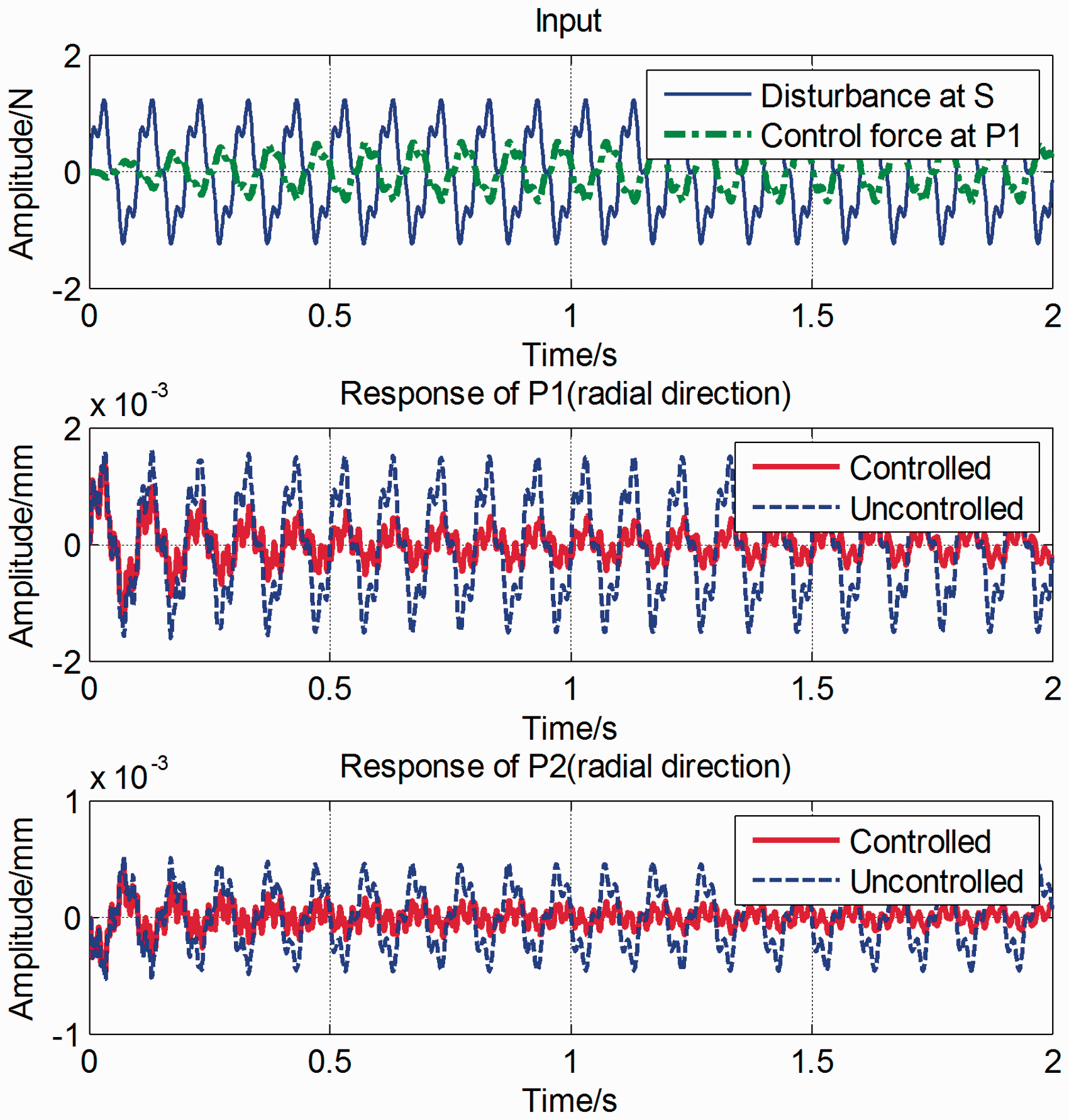

5. Conclusion

Active vibration control of a joint model of a clamped-free shell and the electrodynamic actuators was studied. The FE method was applied to model the joint model and the optimal configuration of the actuators and sensors were also studied. The simulation of AVC was carried out by using the FXLMS algorithm. It can be concluded that the connections of the actuators diminish the natural frequencies and smooth the resonance peaks of the structure. Secondly, it is better to avoid the central line (where the nodal line is) and to give priority to the free end or to the edges of the clamped-free shell when mounting actuators and sensors. Moreover, the FXLMS algorithm is able to suppress multi-frequency and amplitude-varying disturbance. Finally, it is important to mention that the simulation process was conducted point by point on the transient response model of the structure and can easily be extended to real life system.

Footnotes

Funding

This work was supported by the National Natural Science Foundation of China (grant number 51225501).

References

Ardekani

Abdulla

(2011) On the stability of adaptation process in active noise control systems. Journal of the Acoustical Society of America 129(1): 173–184.

Ardekani

Abdulla

(2012) Effects of imperfect secondary path modeling on adaptive active noise control systems. IEEE Transactions on Control Systems Technology 20(5): 1252–1262.

Bai

Chen

(2013) A symplectic eigenfunction expansion approach for free vibration solutions of rectangular Kirchhoff plates. Journal of Vibration and Control 19(8): 1208–1215.

Cao

Liu

Brown

(2008) State of the art in vehicle active suspension adaptive control systems based on intelligent methodologies. IEEE Transactions on Intelligent Transportation Systems 9(3): 392–405.

Cook

Malkus

Plesha

(1989) Concepts and Applications of Finite Element Analysis, Toronto, Canada: John Wiley & Sons, Inc.

Datta

Sokolov

(2009) Quadratic inverse eigenvalue problems, active vibration control and model updating. Applied and Computational Mathematics 8(2): 170–191.

Fung

Liu

Wang

(2005) Dynamic model of an electromagnetic actuator for vibration control of a cantilever beam with a tip mass. Journal of Sound and Vibration 288(4–5): 957–980.

Gardonio

(2002) Review of active techniques for aerospace vibro-acoustic control. Journal of Aircraft 39(2): 206–214.

Gonzalez

Rossi

Molina

Parlanti

(2013) FXLMS and MFXLMS stability constrains when used in active noise control. IEEE Latin America Transactions 11(1SI): 213–217.

10.

Song

(2007) Active vibration suppression of a flexible beam with piezoceramic patches using robust model reference control. Smart Materials and Structures 16(4): 1453–1459.

11.

Hosseini

Arzanpour

Golnaraghi

Parameswaran

(2013) Solenoid actuator design and modeling with application in engine vibration isolators. Journal of Vibration and Control 19(7): 1015–1023.

12.

Jian

Yegui

Jinwei

(2010) Analysis of online secondary-path modeling with auxiliary noise scaled by residual noise signal. IEEE Transactions on Audio, Speech, and Language Processing 18(8): 1978–1993.

13.

Kapuria

Yasin

(2010a) Active vibration control of piezoelectric laminated beams with electroded actuators and sensors using an efficient finite element involving an electric node. Smart Materials and Structures 19(4): 045019(15pp).

14.

Kapuria

Yasin

(2010b) Active vibration suppression of multilayered plates integrated with piezoelectric fiber reinforced composites using an efficient finite element model. Journal of Sound and Vibration 329(16): 3247–3265.

15.

Karagulle

Malgaca

Oktem

(2004) Analysis of active vibration control in smart structures by ANSYS. Smart Materials and Structures 13(4): 661–667.

16.

Khot

Yelve

(2011) Modeling and response analysis of dynamic systems by using ANSYS (c) and MATLAB (c). Journal of Vibration and Control 17(6): 953–958.

17.

Khot

Yelve

Tomar

Desai

Vittal

(2012) Active vibration control of cantilever beam by using PID based output feedback controller. Journal of Vibration and Control 18(3): 366–372.

18.

Korkmaz

(2011) A review of active structural control: challenges for engineering informatics. Computers and Structures 89(23–24): 2113–2132.

19.

Liu

Chen

(2009) Numerical analysis of immersed finite cylindrical shells using a coupled BEM/FEM and spatial spectrum approach. Applied Acoustics 70(2): 256–266.

20.

Malgaca

(2010) Integration of active vibration control methods with finite element models of smart laminated composite structures. Composite Structures 92(7): 1651–1663.

21.

Malgaca

Karagulle

(2009) Numerical and experimental study on integration of control actions into the finite element solutions in smart structures. Shock and Vibration 16(4): 401–415.

22.

Meng

Dong

Wei

(2006) Closed loop finite element modeling of piezoelectric smart structures. Shock and Vibration 13(1): 1–12.

23.

Park

Lee

(2012) Dynamic analysis of smart composite beams by using the frequency-domain spectral element method. Journal of Mechanical Science and Technology 26(8): 2511–2521.

24.

Song

Sethi

(2006) Vibration control of civil structures using piezoceramic smart materials: A review. Engineering Structures 28(11): 1513–1524.

25.

Tong

Zhang

Hua

(2007) Dynamic behavior and sound transmission analysis of a fluid-structure coupled system using the direct-BEM/FEM. Journal of Sound and Vibration 299(3): 645–655.

26.

Koko

(2004) Finite element analysis and design of actively controlled piezoelectric smart structures. Finite Elements in Analysis and Design 40(3): 241–262.

27.

Zienkiewicz

Taylor

(2005) The Finite Element Method for Solid and Structural Mechanics, 6th edn. Burlington, MA: Butterworth-Heinemann.