
Abstract
This paper proposes a multiclass nonlinear relevance vector machine (MNRVM) model for health monitoring of smart structures equipped with magnetorheological (MR) dampers. The proposed model will be used to classify the damage statuses of the integrated structure-control systems subjected to ambient excitations. A numerical model of a three-story building equipped with an MR damper is studied to demonstrate the effectiveness of the proposed health monitoring schemes. Dynamic responses of the smart structures subjected to random excitations are measured. Discrete wavelet transform is applied to the obtained data to compress and filter noises of the measured data. As a next step, the compressed and de-noised signals are used for developing autoregressive (AR) models. Then the MNRVM is applied to the AR-coefficient data to classify them with respect to the damage statuses. As a baseline, the support vector machine (SVM) algorithm is considered. It is demonstrated that the proposed MNRVM framework is effective in classifying various damage statuses of the nonlinear smart structures subjected to ambient excitations. Simulation results also show that the MNRVM performs similar to the SVM with faster computation time.
Keywords
1. Introduction
Structural health monitoring (SHM) systems have received much attention in the civil engineering field (Worden and Lane, 2001; Mita and Hagiwara, 2003; Bulut et al., 2005, Huang et al., 2011; Kim et al., 2013). In particular, SHM assists engineers to detect structural damage proactively with non-destructive testing by providing real-time monitoring systems (Farrar and Worden, 2007). For example, when the structure is excited by a natural or man-made hazard, the properties of a structural system such as stiffness and damping may change. The measured changes that are observed by sensors may alert the SHM system. Then, the SHM provides real-time information to identify the location and severity of the damage which can work as a proactive warning mechanism (Figueiredo et al., 2012). However, it would be challenging for such damage detection approaches to be applied to smart structures due to the highly complicated nonlinear behavior of integrated structure smart control systems.
One of the promising methods to classify and evaluate the highly nonlinear structural responses obtained from integrated structure-control systems would be to use the support vector machine (SVM) framework (Kim et al., 2013). In general, the SVM uses the statistical learning theory to transform the data to a higher dimensional feature space and find the optimal hyperplane in the space that maximizes the margin between classes (Burges, 1998; Hou et al., 2011; Mohammadnejad et al., 2011). The SVM has recently been applied to the civil engineering field. Worden and Lane (2001) applied the SVM in the investigation of the vibration-based damage of truss structures. Another application was performed by Mita and Hagiwara (2003) in the damage detection of shear type building structures. In the study, the changes in the model frequency of the structure were observed and an SVM was adopted to determine the local damage. Shimada and Mita (2005) applied an SVM framework to a damage assessment system of bending structures. They verified the performance of the SVM using analytical models and experiments. It was demonstrated that the SVM is effective in detecting damage in bending structures. Oh and Sohn (2009) evaluated the effectiveness of an SVM in structural damage detection in the presence of an unmeasured operational variation. It has also been demonstrated from previous studies that the SVM can be effective in classifying the damage on bridge structures (Bulut et al., 2005, Park et al., 2006, Vines-Cavanaugh et al., 2010). Bulut et al. (2005) focused on the damage detection of the Humboldt Bay Middle Channel Bridge by using an SVM classifier. Another study was performed on detection of abnormality on a cable-stayed bridge structure (Vines-Cavanaugh et al. 2010). Damage statuses of the expension joints were classified by an SVM. Park et al. (2006) proposed a nonlinear SVM-based binary classification for damage detection of small-scale steel bridge components. The maximum peak values at a specific frequency were compared to show the efficiency of the SVM.
However, the main focus of all of the aforementioned studies was on the linear behavior of uncontrolled linear dynamic systems, not highly nonlinear behavior of complex structure smart control systems. Although the SVM is one of the most effective classification processes, Tipping (2001) stated that the accuracy of the SVM classification can decrease significantly when it is trained using small datasets. Furthermore, since the SVM considers optimal selection for penalty term and kernel parameters (Foody, 2008), finding optimal parameters is computationally expensive (Tipping, 2001).
On the other hand, the relevance vector machine (RVM), which is a Bayesian extension of the SVM, can be considered as an alternative method. There are previous studies that used the RVM as an alternative to the SVM. The study of Xiang-min et al. (2007) in the bioengineering field was mainly focused on the comparison of SVM and RVM models. They demonstrated that the performance of RVM in terms of generalization and decision speed was better, while the training efficiency and classification accuracy of the RVM was similar to that of the SVM. Foody (2008) used the RVM in the multi-class classification of an agricultural test site. However, there is only one study about the RVM in the civil engineering field (Huang et al., 2011). The study was focused on a Bayesian formalism, which was based on the RVM, to compress the data obtained from SHM systems. They proposed diagnostic tools to investigate whether the compressed representation of the signal was optimal. However, the main purpose of the study was to decrease the data transfer cost by compressing the signals obtained from SHM systems, not the damage classification of highly nonlinear smart structure systems. As of yet, there is no research on the RVM that has proposed to classify the damage of smart structures. With this in mind, an RVM-based structural health monitoring framework for damage detection of structures equipped with time-varying hysteretic control devices is proposed so that the nonlinear behavior of integrated structure smart control systems is effectively classified in this paper.
This paper is organized as follows: Section 2 discusses the SVM and RVM in detail. Discrete wavelet transforms (DWT), autoregressive (AR) model and damage sensitive features are also discussed in Section 2. In Section 3, the case study and its procedures are described. The binary and multi-class classification results, including comparison of the SVM and RVM, are given in Section 4. Concluding remarks are given in Section 5.
2. Multiclass nonlinear relevance vector machine (MNRVM)
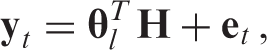
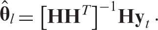
The data generation, regression and classification process is depicted in Figure 1. For the classification process, the multiclass nonlinear relevance vector machine (MNRVM) is considered in this paper. In order to obtain data for training and validating the RVM, a scaled three-story smart building equipped with an MR damper is studied. The properties of the three-story building structure are adopted from a scaled building model (Dyke et al., 1996) of a prototype building structure that was developed by Chung et al. (1989). The structural system is subjected to random excitation and random current values on the MR damper. Acceleration, velocity and displacement of the smart structure are obtained. First, DWT is applied to selected datasets in order to compress and denoise them. As a second step, the AR model estimates the filtered response and constructs wavelet-based AR (WAR). As a third step, MNRVM classifies the WAR data into either healthy or damaged status. In the MNRVM classification, one part of the WAR data is used to train the data, while the other part is applied to the validation process.
Architecture of the proposed relevance vector machine scheme for smart structures.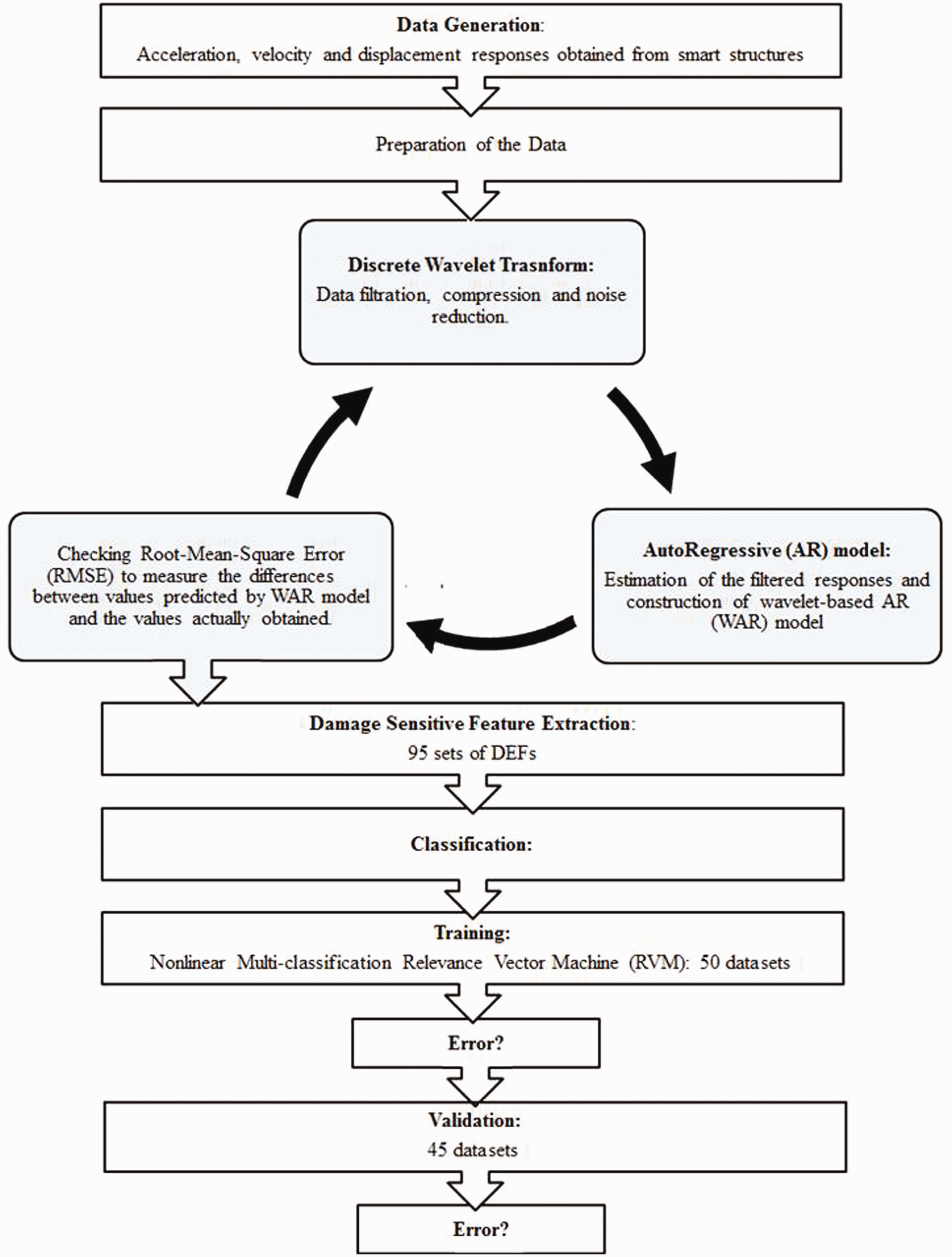
The SVM that will be used as a benchmark is described first in the following section, and then the proposed RVM is presented.
2.1. Support vector machine (SVM)
In general, the SVM classifier finds the support vectors which maximize the margin (or the distance) by using training data. The linear SVM can be categorized into soft margin SVM and hard margin SVM. The soft margin SVM is for the datasets which are mixed and cannot be separated into classes. On the other hand, hard margin SVM is usually applied to the situation where the data points are separable. The hard margin SVM uses the following equation to find the support vectors.

In the soft margin SVM algorithm, slack variables are introduced to minimize the error and maximize the margin. To determine the decision boundary of the soft margin SVM, the following equations are used


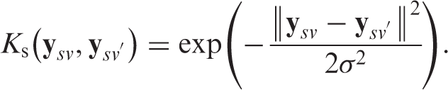
To facilitate the operation in nonlinear SVM, a kernel function Ks, which is a dot-product in the transformed feature space as follows, is used

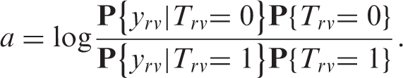
Using an appropriate kernel function that satisfies the Mercer’s condition and non-probabilistic estimations are drawbacks of the SVM. Furthermore, the usage of error/margin tradeoff parameters (δ sv and Cs) during the cross-validation process results in data loss and increased computation time. Thus, in order to decrease the computation time and prevent data loss, an RVM approach is adopted that decreases the computation time while maintaining accuracy.
2.2. Relevance vector machine (RVM)
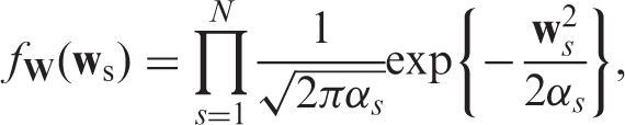
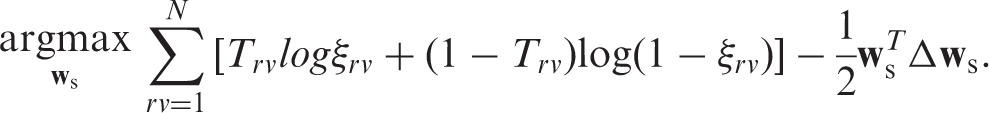
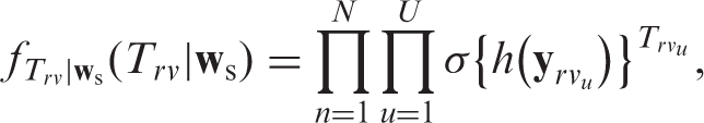
The RVM estimates the class of given input by calculating the probability of membership for pre-defined classes. Hence, it is straightforward to incorporate uncertainties into classification procedure using RVM. It is noted that it is difficult to express the uncertainties in the SVM because the outputs of SVM are deterministic values. Thus, many uncertain variables need to be iteratively updated using all possible C. Moreover, the kernel function of the SVM needs to be the semi-positive definite condition. On the other hand, since the RVM does not require the parameter C to be defined, it reduces sensitivity to the hyperparameter settings. It has a probabilistic output (Mahesh, 2009). Thus a new RVM approach, which is much sparser and faster when compared to that of the SVM, is proposed to classify the damage on smart structures in this paper. The linear form of an RVM classifier is considered as

The process starts by training the RVM classifier. The RVM is trained with an input dataset to obtain the optimum parameters for the RVM classifier. In this case, the RVM classifier separates the input data into the healthy and damaged (5%, 10%, 15%, 30% and 50%) signals.
Similar to the SVM, the training dataset consists of the training input data and its target variables, which are defined as

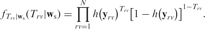
The likelihood function of training data for two class classification can be written as
Since
The RVM is trained and validated with the WAR coefficients, which is the integration of DWT and AR. Both DWT and AR model is described in detail in the following sections.
2.3. Discrete wavelet transforms (DWT)
The DWT decomposes the given signal into several levels of subcomponents and then reconstructs them into the original signal to compress the data and reduce the noise (Thuillard, 2001). A continuous WT can be represented as
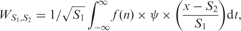
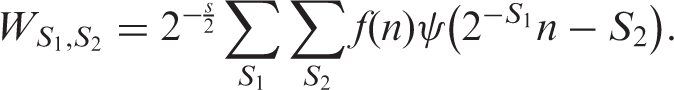
As a time frequency analysis method, DWT isolates the high frequency components from the original signal. In order to investigate both high and low frequency signals, DWT can be utilized for multi-resolution analysis (MRA). The MRA decomposes the time-series signals obtained from the smart structure into both low and high frequency components at different resolutions (Kim et al., 2013). The scaling function φ and the corresponding wavelet ψ are defined as follows
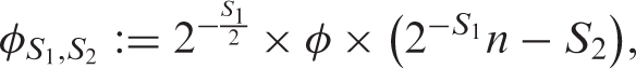
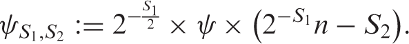
The scaling function acts as a low pass filter for filtering the data from high frequencies, while the corresponding wavelet filters the lower frequencies. As a useful tool to filter the data and decompose the time series in terms of time and frequency, DWT is applied to the AR model in order to increase the modeling efficiency.
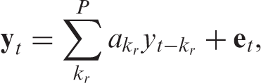
2.4. Autoregressive (AR) model
The objective of the AR model is to estimate the behavior of the structural dynamic system by using the obtained responses from the smart structure. In particular, the AR model is given by
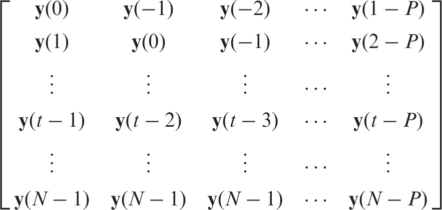
Minimization of the criterion function with respect to
From the obtained coefficients,
2.5. Wavelet-based AR model (WAR)
In the classification process of the RVM, WAR models are used. As discussed in previous sections, the DWT is an effective tool to decompose time series into subseries in terms of time and frequency. Thus, it increases the efficiency of the time-series modeling, by integrating DWT with the AR model. The WAR can be derived by modifying equation (20) as
The WAR model uses level 2 wavelet filtered signals. The WAR coefficients are transformed into a set of poles to perform structural damage detection of smart structures.
2.6. Pole location identification
Using Z-transform, the WAR coefficients can be transformed into a set of poles (Nair et al., 2006).
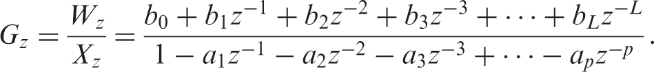
The denominator of the transfer function Gz is a characteristic equation of order P. By solving the root of the denominator, the system poles can be obtained as

When a structure has changes on the properties of structural systems, they can be quantitatively measured by the migration patterns of the transfer function poles (Nair et al., 2006). To this end, a damage sensitive feature (DSF) is proposed to capture the changes of the AR coefficients obtained from undamaged to damaged structural systems.
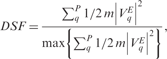
2.7. Damage-sensitive feature extraction
In the discrimination between healthy and damaged structures, a new DSF is used. In particular, the DSF is extracted by normalizing the WAR coefficients. In this study the DSF is obtained by normalizing the WAR coefficients using a pseudo energy expression with velocity responses. Thus, the proposed DSF is determined as follows
3. Case study: smart structures
3.1. Magnetorheological (MR) damper
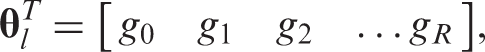
In recent years, MR dampers have received great attention with the increase of smart structure applications in many engineering fields as shown in Figure 2. Magnetorheological dampers combine the best features of both passive and active control systems (Spencer et al., 1997; Kim et al., 2009). In particular, MR dampers work as a semi-active system with the application of a magnetic field to the MR fluid. The magnetic field affects the rheological and flow properties of the MR fluid to absorb and dissipate energy effectively. On the other hand, without any current on the system, MR dampers turn to a passive damper. The integration of the MR damper technology with the structure is described in the following section.
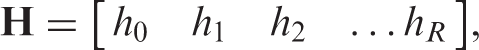
Schematic of magnetorheological damper.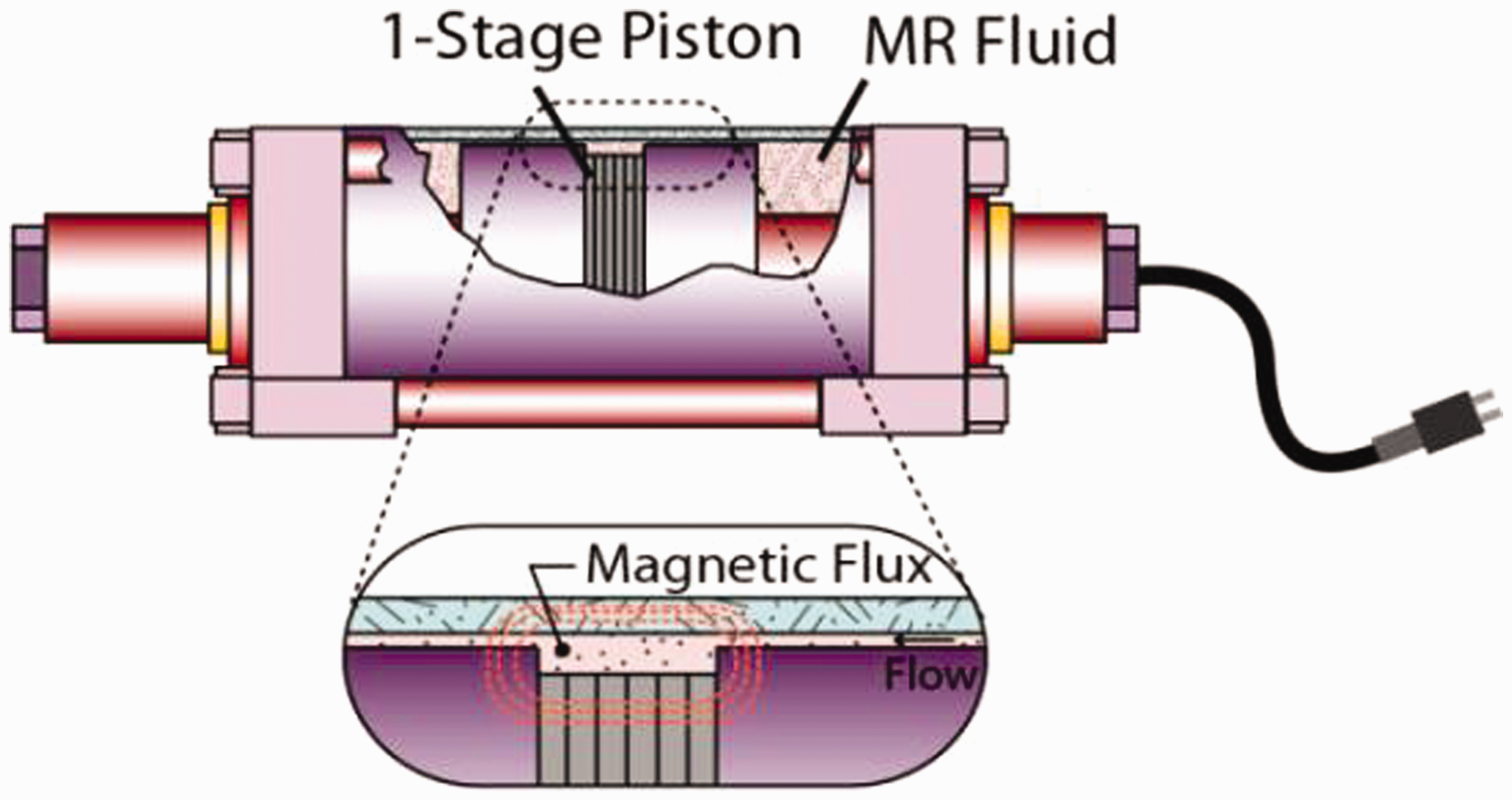
3.2. A building equipped with a magnetorheological (MR) damper
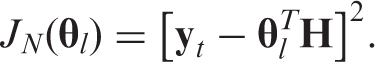
A typical example of an integrated structure-MR damper is shown in Figure 3.
Smart building equipped with an magnetorheological damper.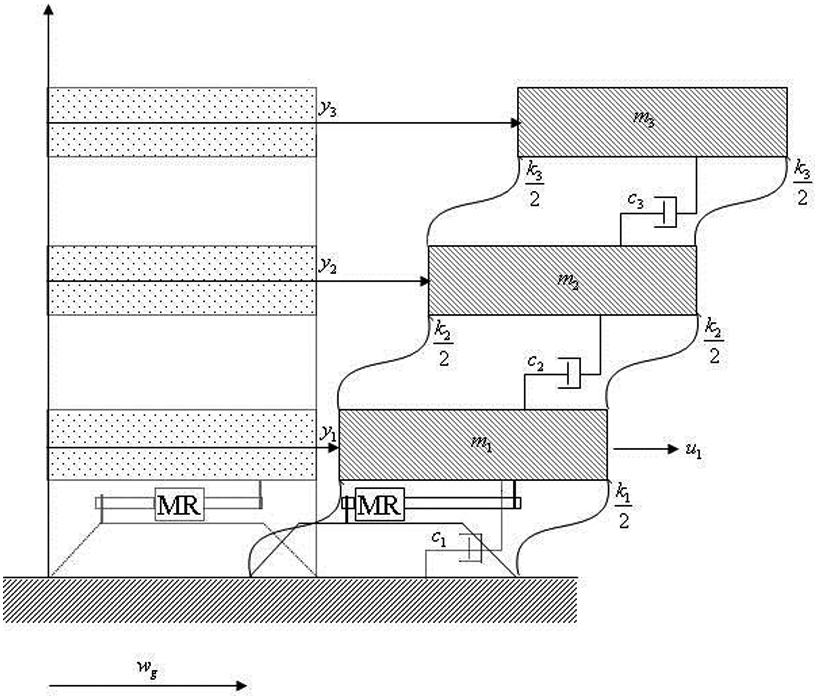
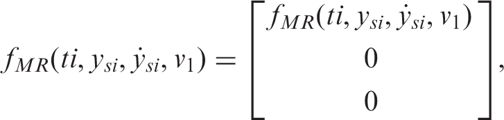
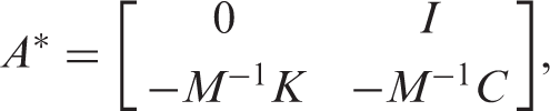
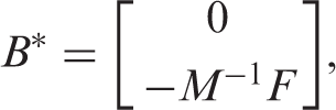
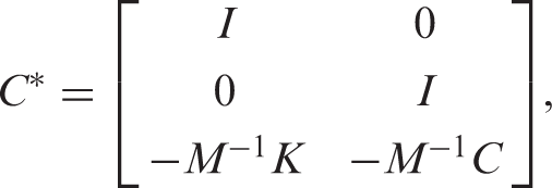
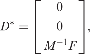
The equation of motion of the integrated smart structure is
Integrated structure-magnetorheological damper system.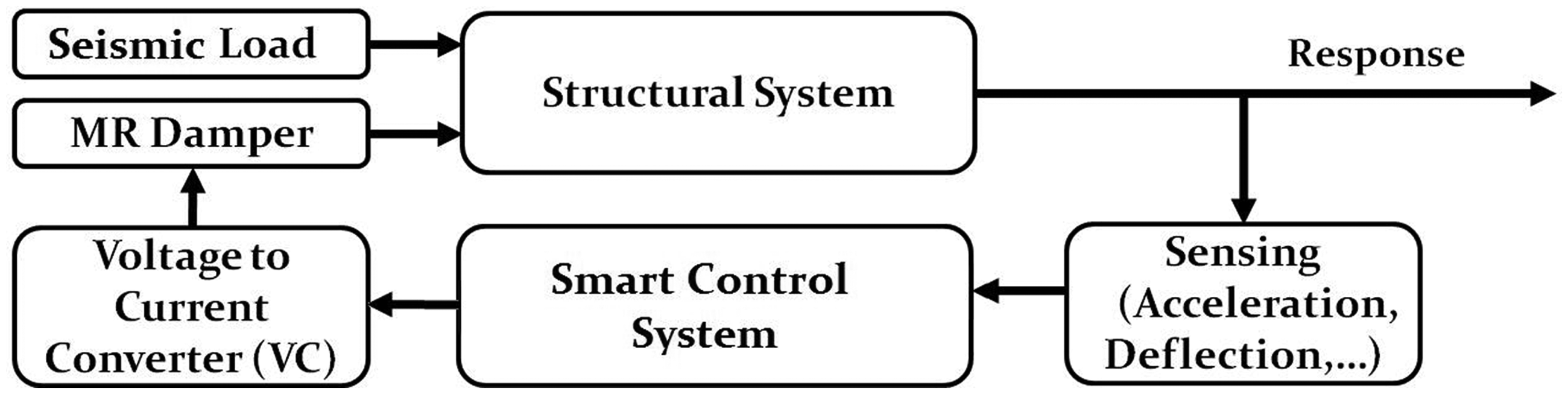

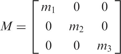
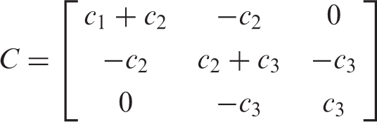
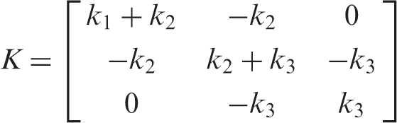


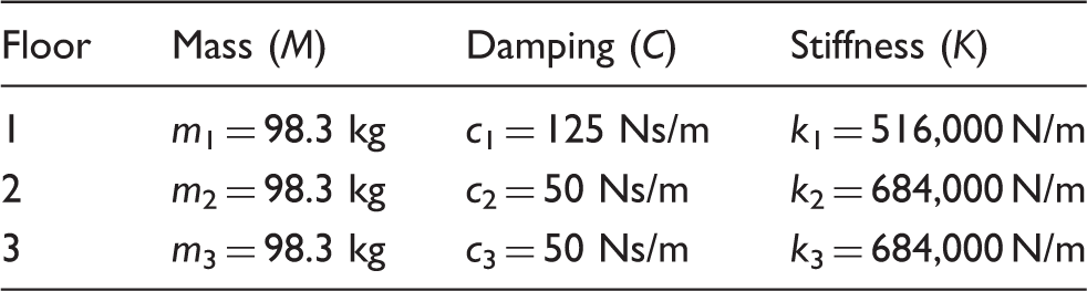
The structural properties of a three-story building structure.
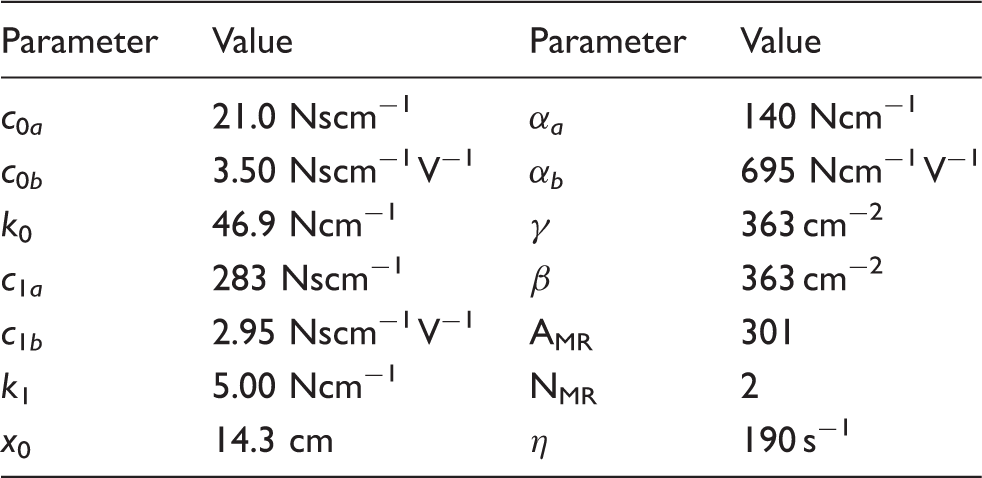
Parameters for SD-1000 magnetorheological damper model.
In order to develop the WAR model, a set of dynamic responses are collected from the smart structure model. The damage scenarios are discussed in the following section.
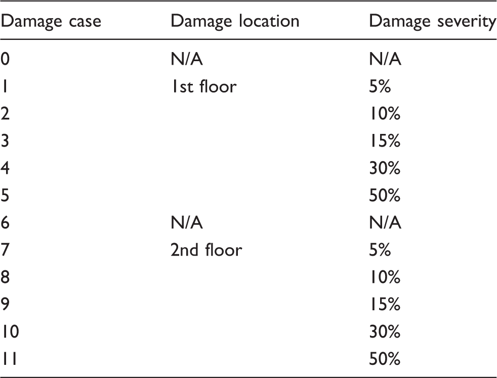
3.3. Damage scenario
Damage scenarios.
3.4. Classification results
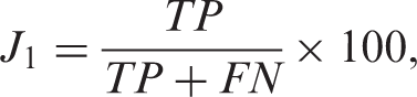
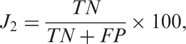
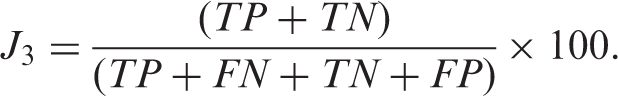
To demonstrate the effectiveness of the proposed RVM approach, binary and multi-class classifications are considered in the paper. To quantify the performance, several evaluation indices are used. As a first evaluation index, sensitivity is calculated as
Numbers of the used support and relevance vectors are defined as the fourth evaluation index.

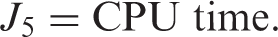
The last evaluation index J5 is assigned as the CPU time to evaluate the duration of the training time.
Following sections evaluates the performances of binary and multi-class classification of the SVM and RVM. It is seen that the RVM classifies the status of the structure accurately with a significantly reduced load of computation compared to the SVM model.
3.5. Two-class classification
In binary classification, the measured data is classified into either healthy or damaged status.
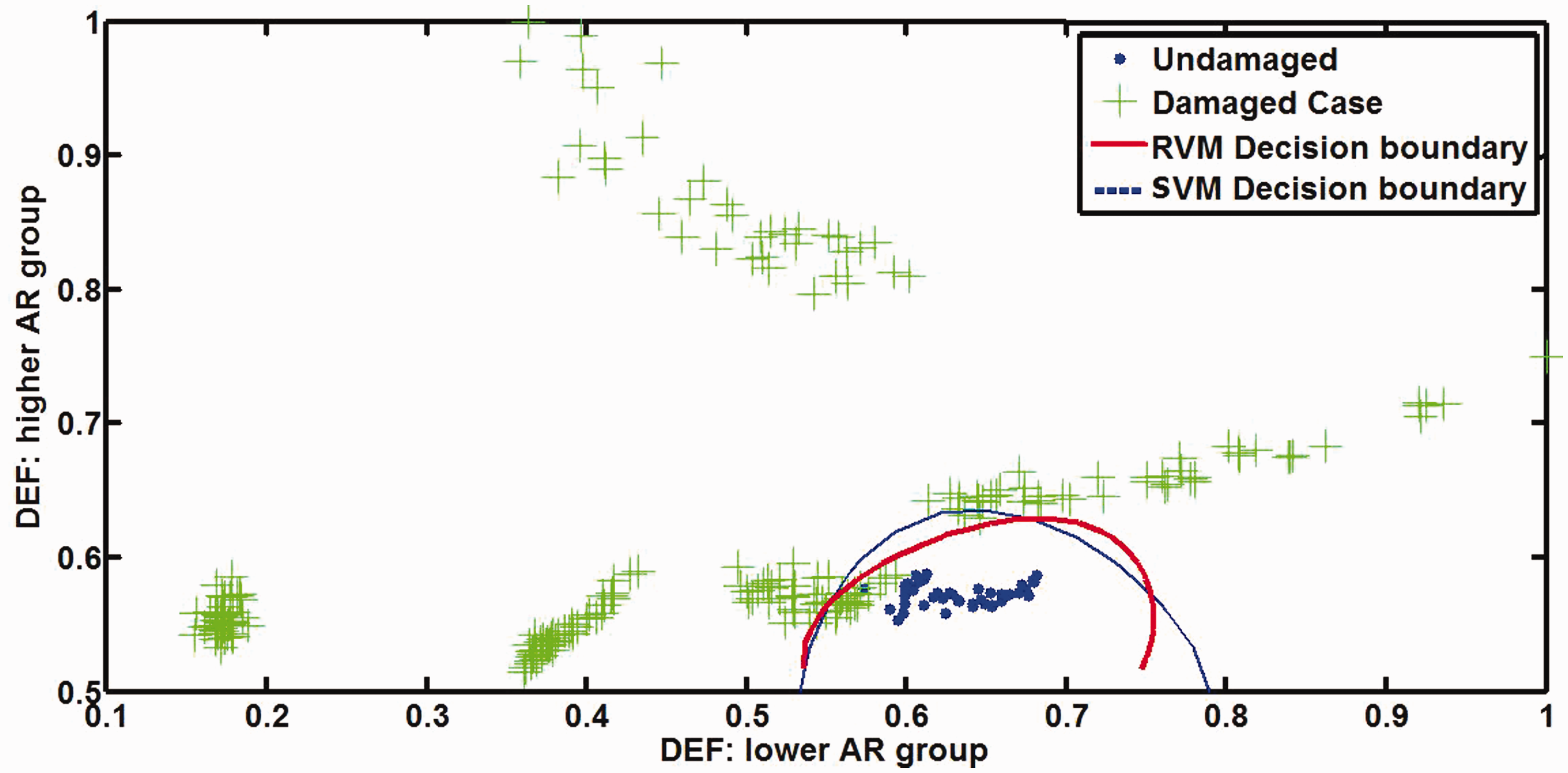
In order to obtain input data for training and validating the SVM and RVM models, 95 DSF are collected for each healthy and each damaged case. To train the models, 100 data points are used. First 50 data of the healthy case and first 10 data from each 5%, 10%, 15%, 30% and 50% damaged statuses are used for training. Then, the models are validated by using 270 data points, which are different from the training data. The models are evaluated by using the last 45 data of the healthy case and the last 45 data of the 5%, 10%, 15%, 30% and 50% damaged statuses. In other words, models are trained with 100 data points (50 for healthy case, 50 for damaged case) and then validated with 270 data (45 for healthy case, 225 for damaged case). Figures 5 and 6 represent the training results while Figures 7 and 8 show the validation of binary SVM and RVM classifications for different floor levels.
Training-binary relevance vector machine and support vector machine: case 0 through case 5. Training-binary relevance vector machine and support vector machine: case 6 through case 10. Validation-binary relevance vector machine and support vector machine: case 0 through case 5. Validation- relevance vector machine and support vector machine: case 6 through case 10.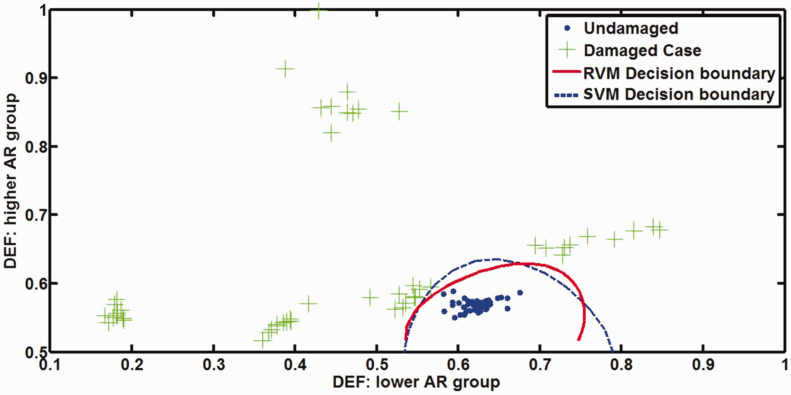
Evaluation indexes of SVM and RVM binary classification.
RVM: relevance vector machine; SVM: support vector machine.
It is observed that both SVM and RVM are effective in the classification of the data into healthy and damaged statuses. However, when the two frameworks are compared in terms of the number of required vectors, the number of required vectors of the RVM is much less than that of the SVM.
3.6. Multi-class classification
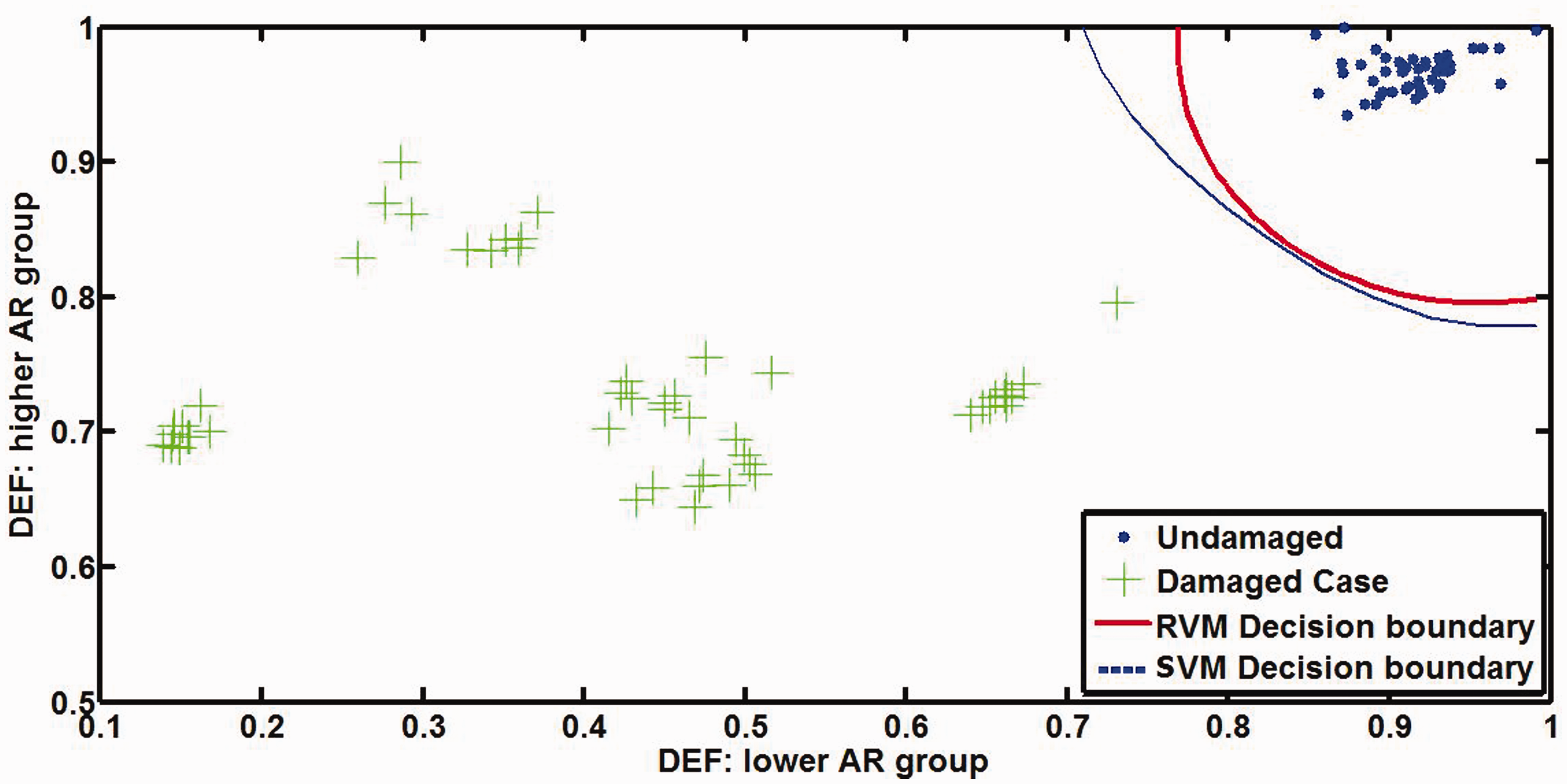
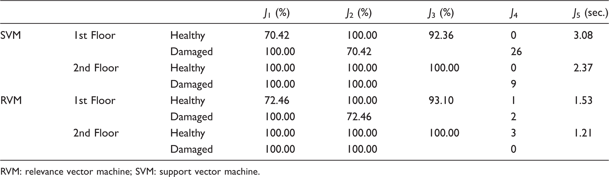
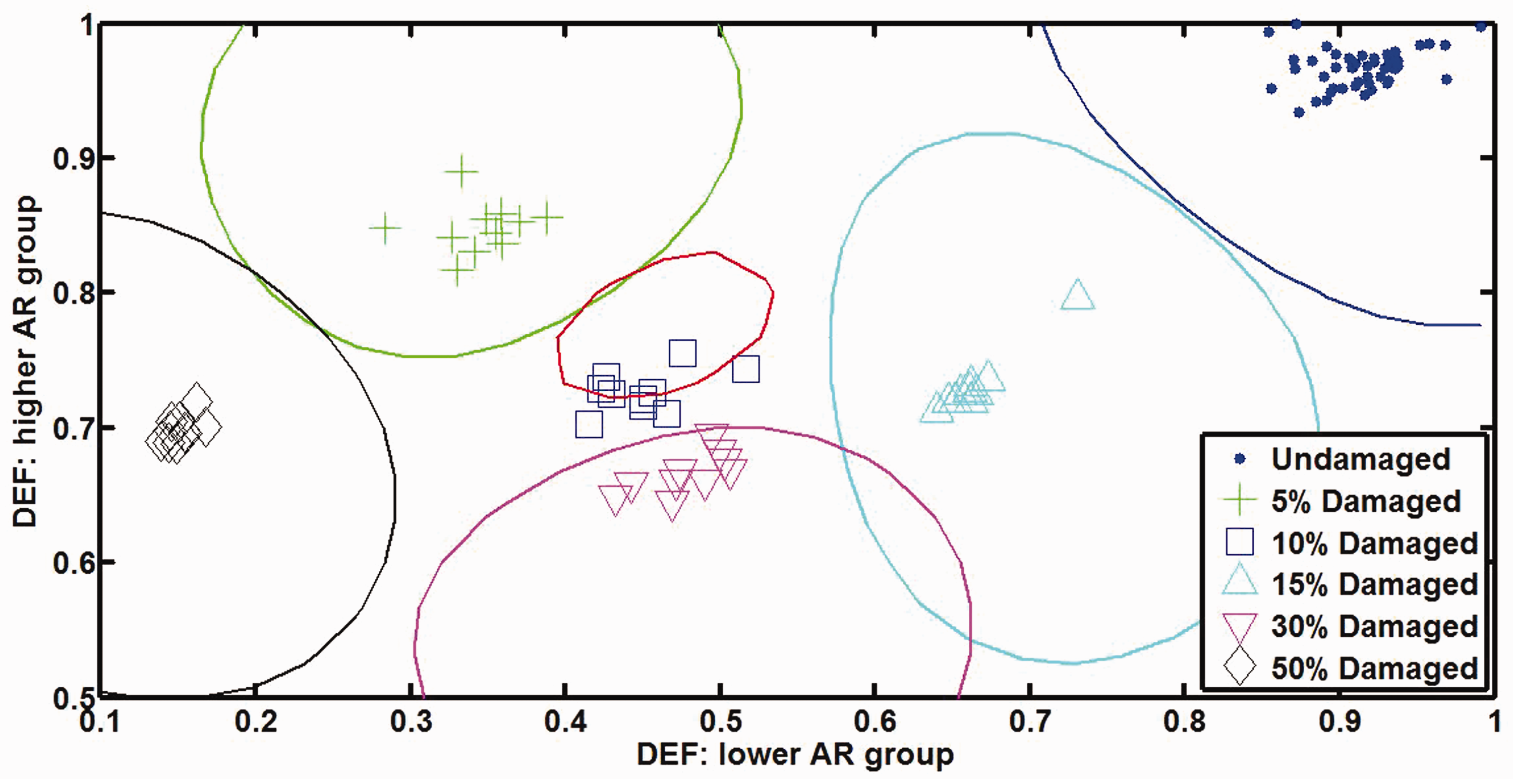
In the training of the multi-class classification, the same training set, which is used in the binary classifications, is used. The measured data is classified into the healthy and damaged (5%, 10%, 15%, 30% and 50%). Models are evaluated by 270 data points (45 for healthy and 45 for each 5%, 10%, 15%, 30% and 50% damaged cases). Figures 9 to 12 represent the training and validation results of the SVM.
Training-multiclass support vector machine: case 0 through case 5. Training-multiclass support vector machine: case 6 through case 10. Validation-multiclass support vector machine: case 0 through case 5. Validation-multiclass support vector machine: case 6 through case 10.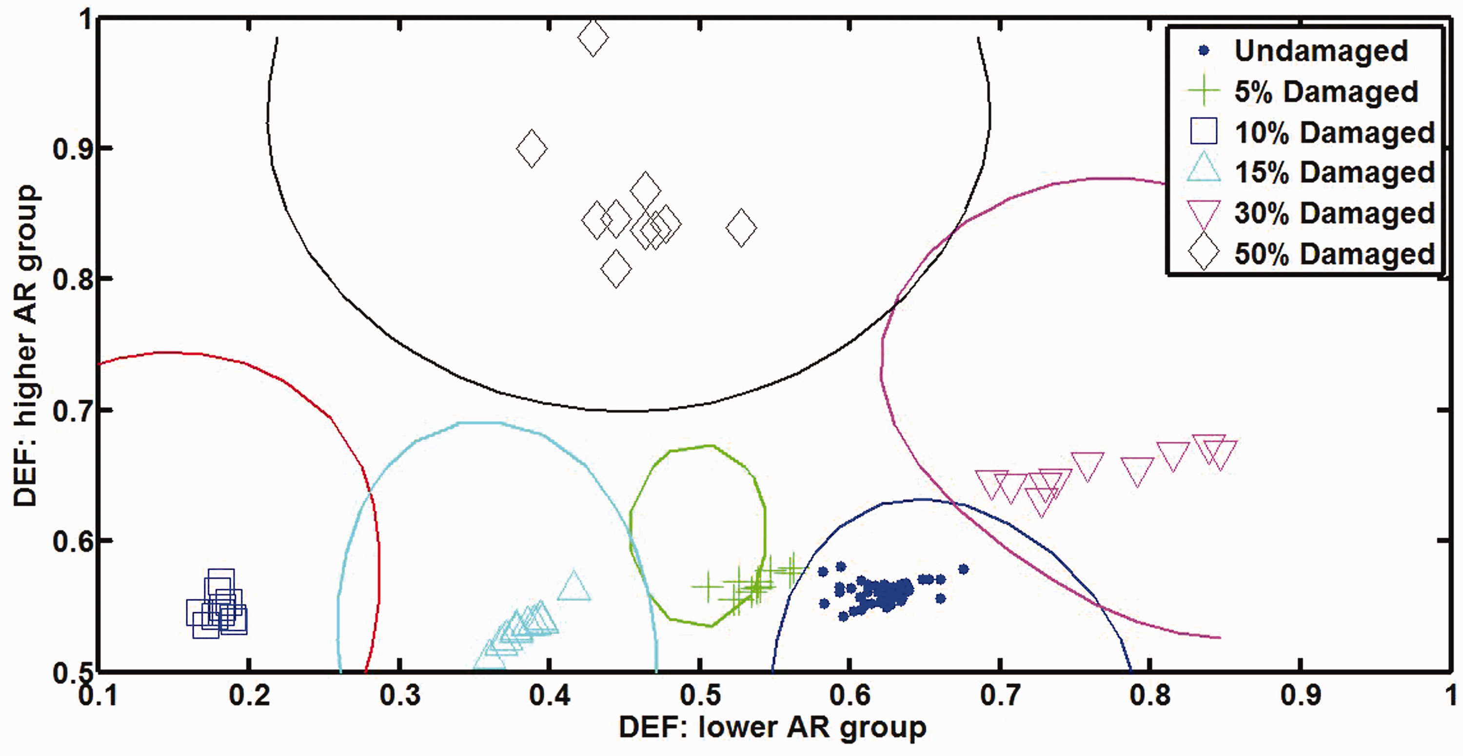
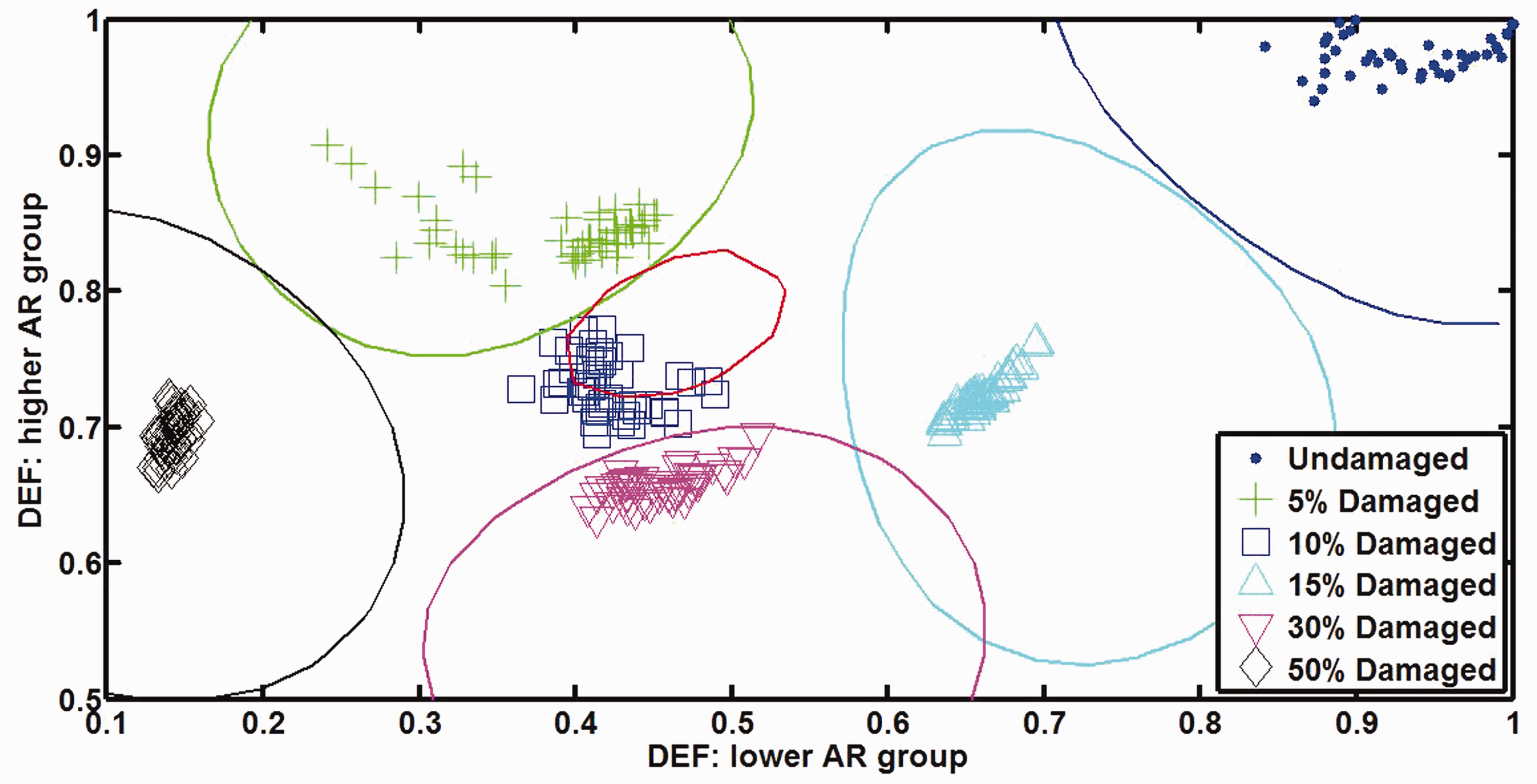
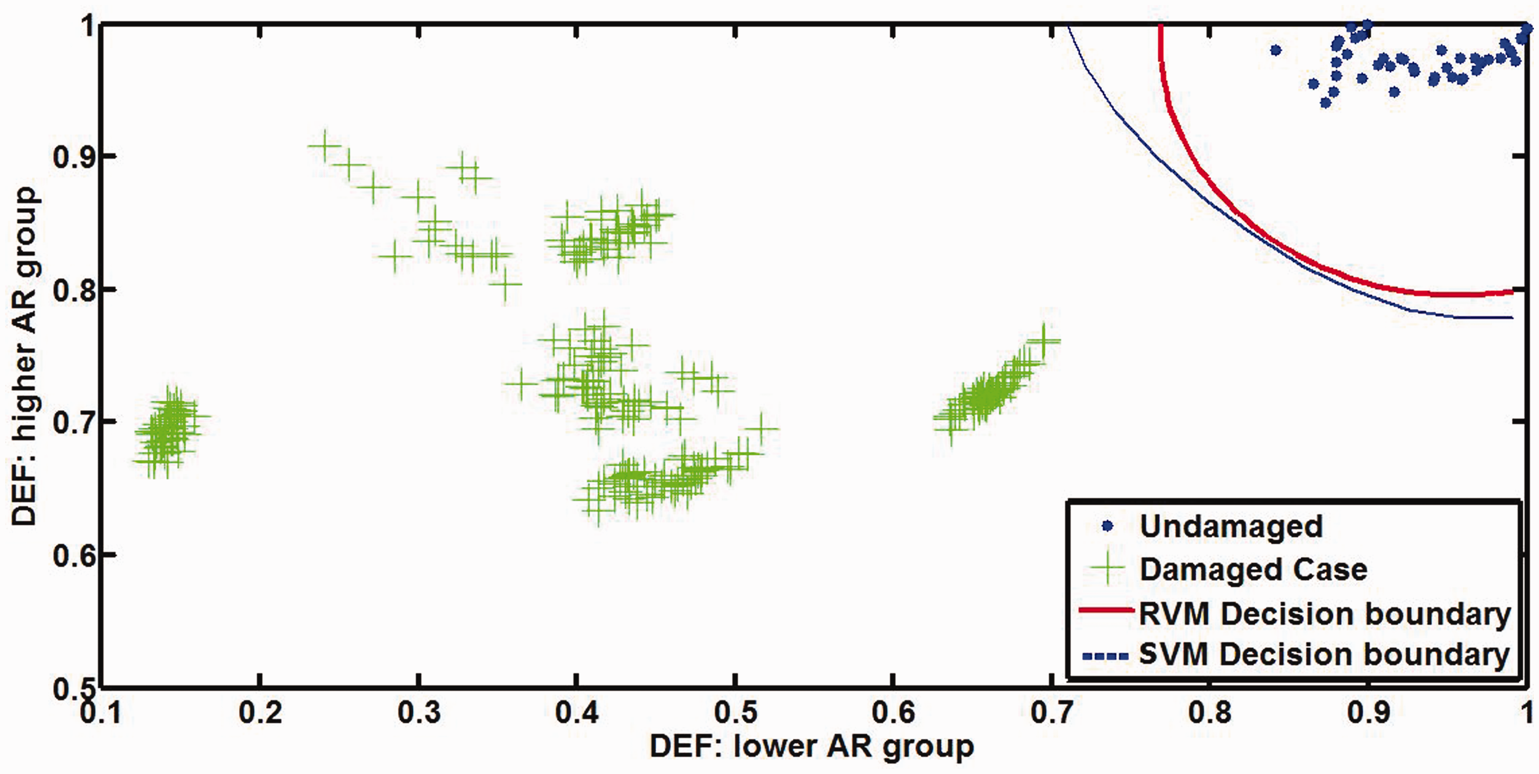
Figures 13 to 16 show the results of the RVM classification.
Training-multiclass relevance vector machine: case 0 through case 5. Training-multiclass relevance vector machine: case 6 through case 10. Validation-multiclass relevance vector machine: case 0 through case 5. Validation-multiclass relevance vector machine: case 6 through case 10.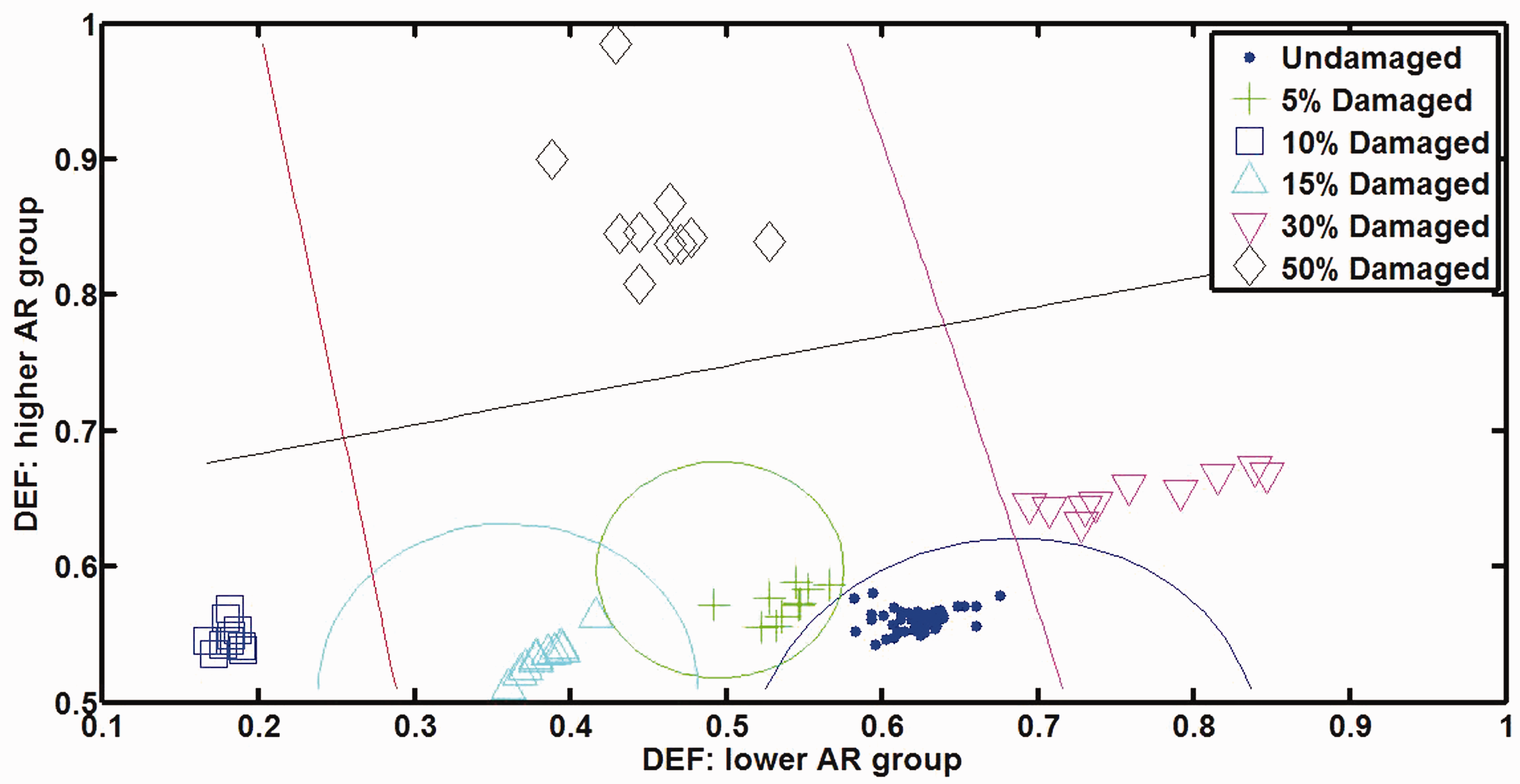

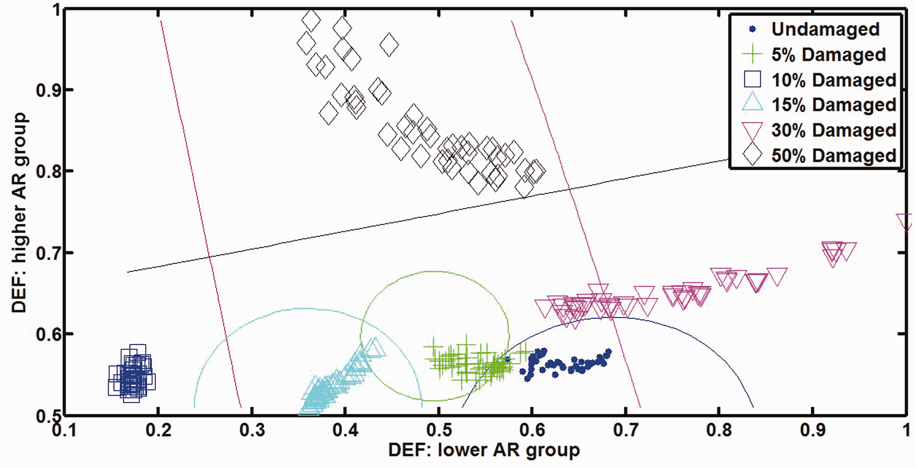
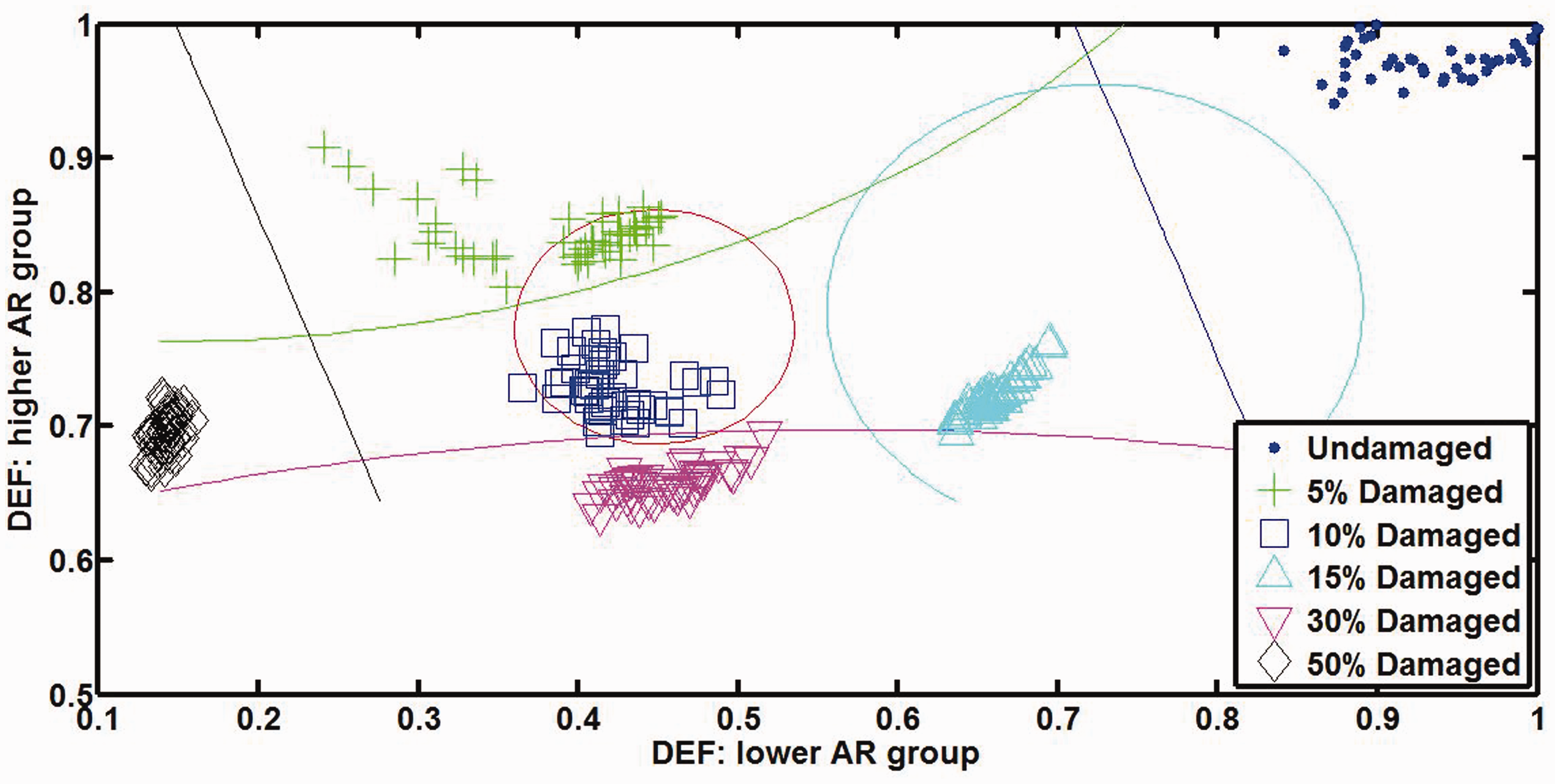
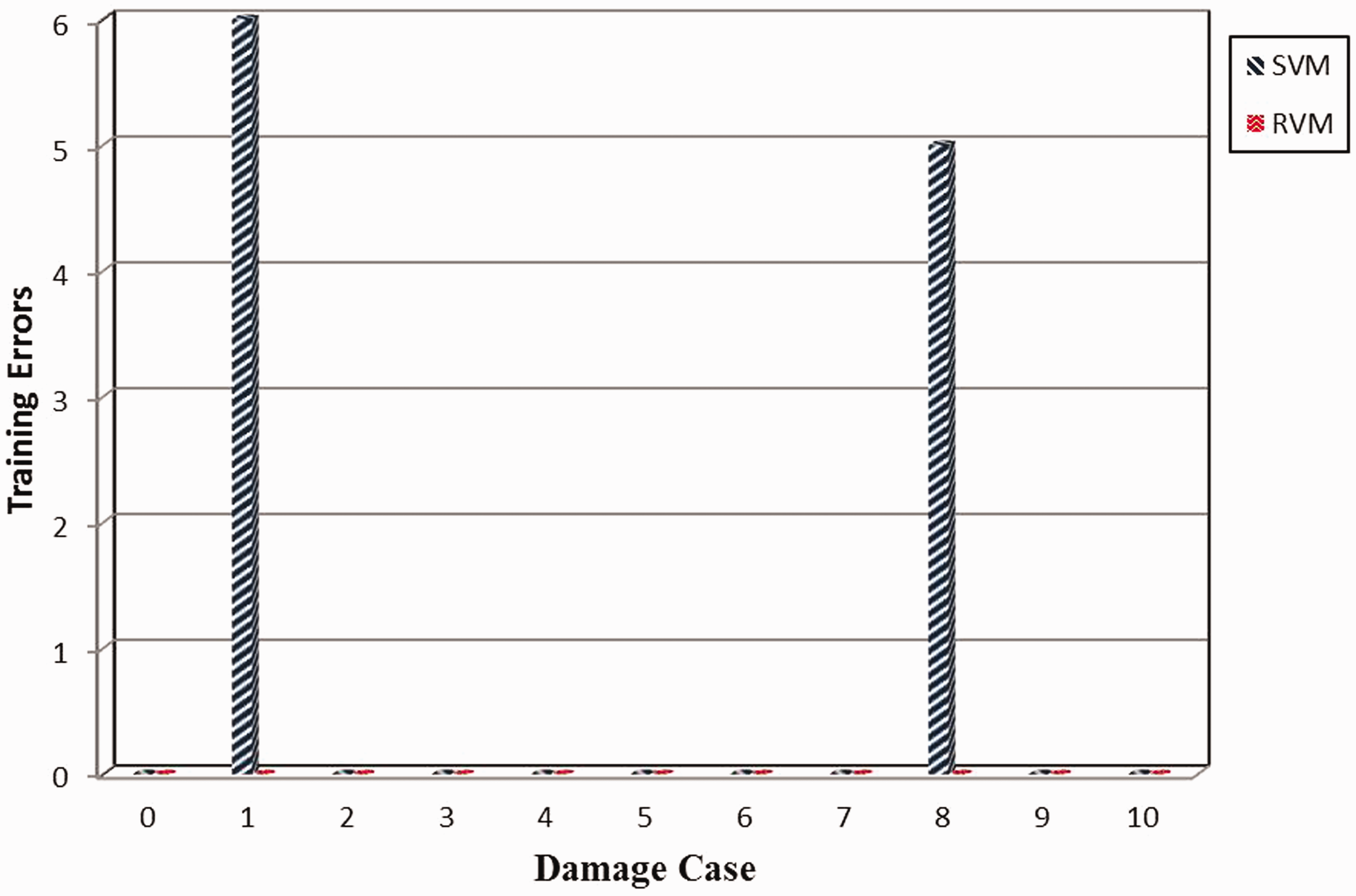
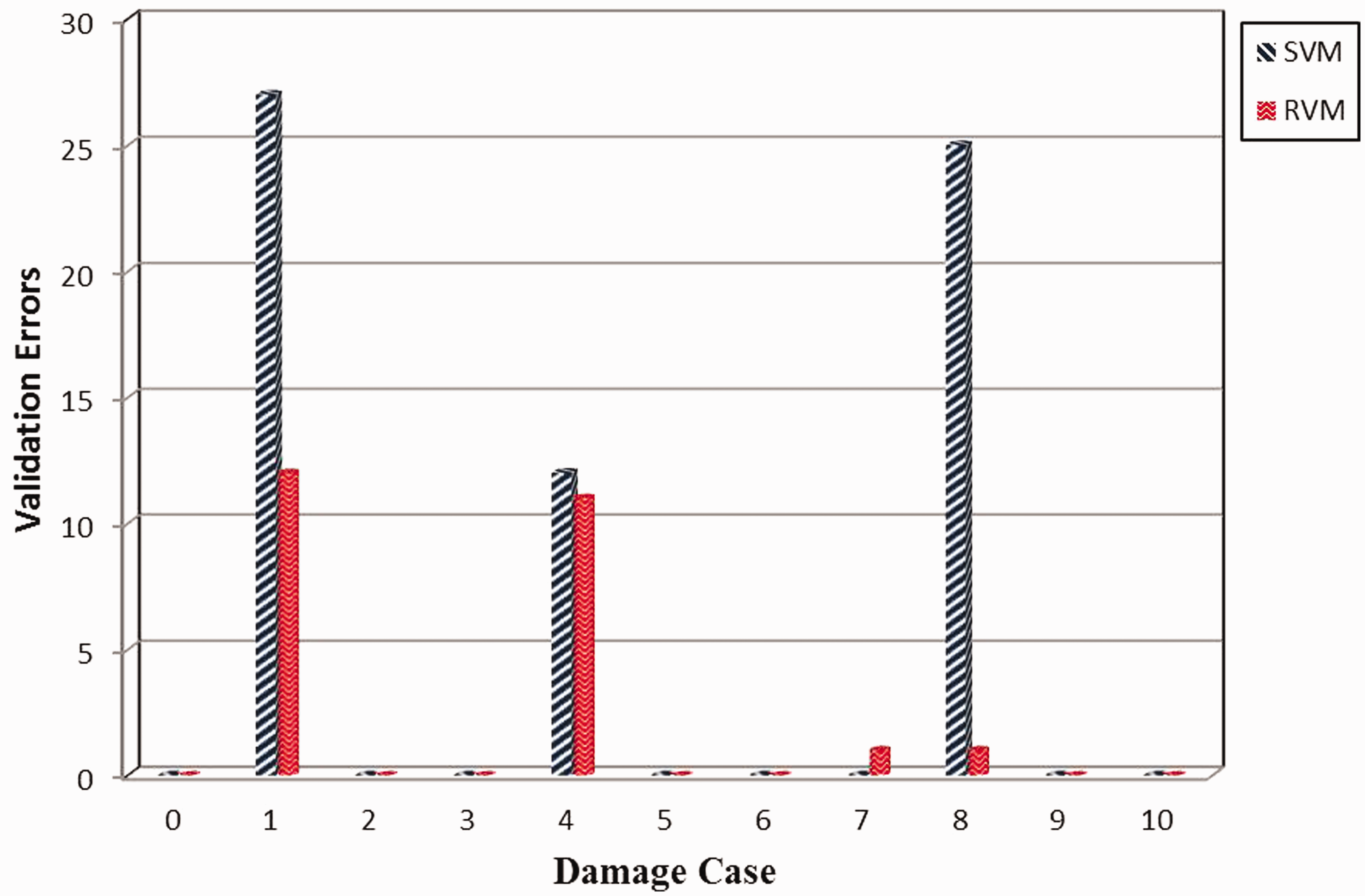
Figure 17 depicts the comparison of the SVM and RVM in terms of number of vectors used in training, while Figure 18 compares the training errors of both approaches. Figure 19 shows the number of validation errors for each damaged status.
Comparison-number of support and relevance vectors for each damage status. Comparison-training errors vectors for each damage status. Comparison-validation errors vectors for each damage status.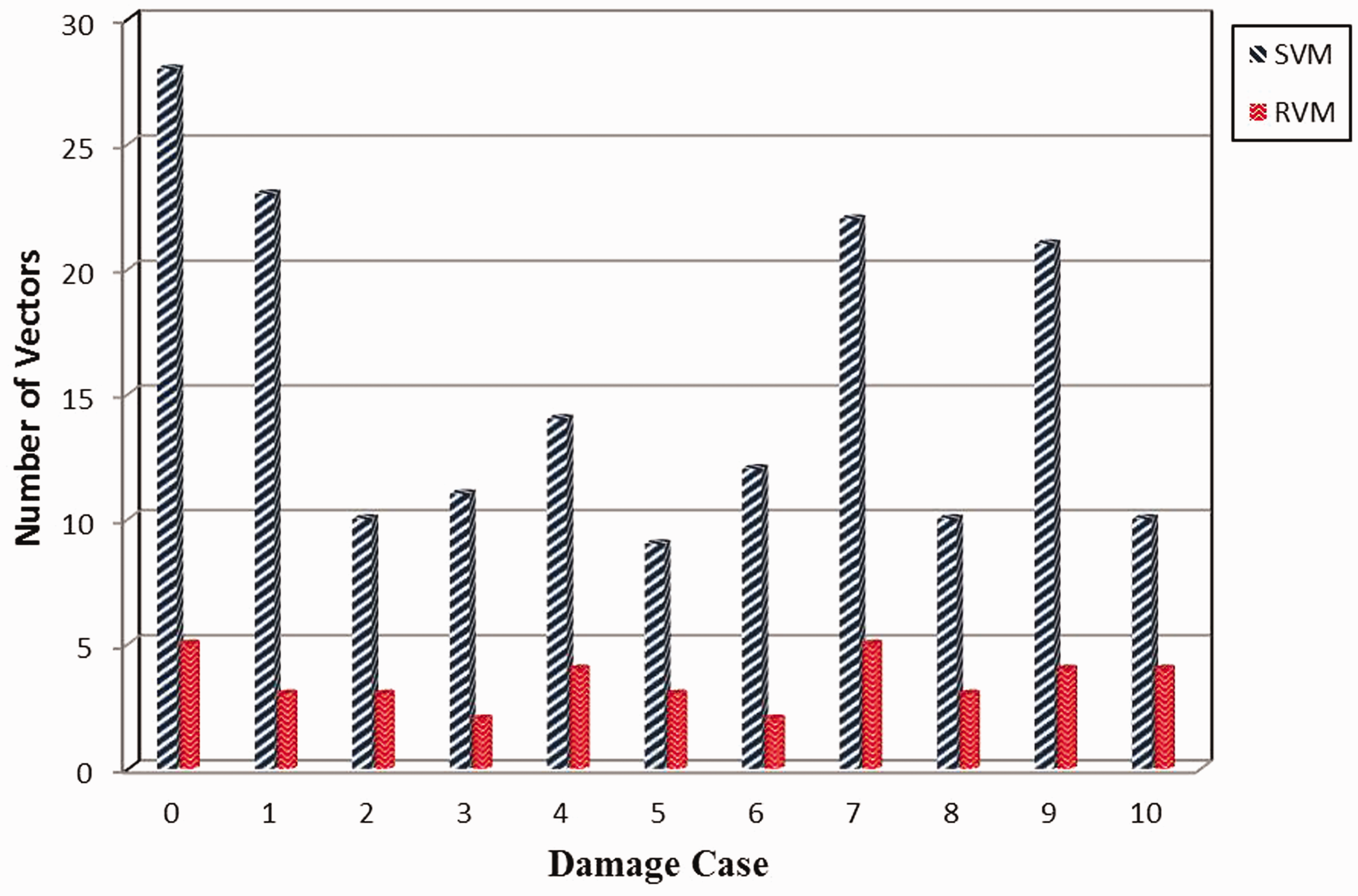
Evaluation of SVM and RVM multi-class classification.
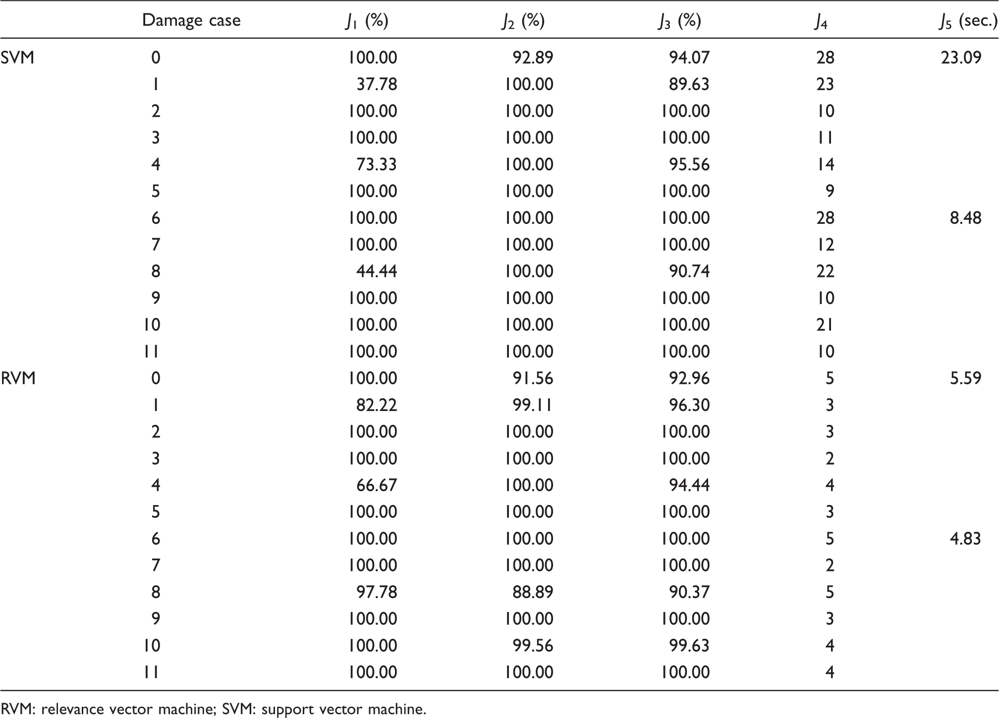
RVM: relevance vector machine; SVM: support vector machine.
It is observed from the simulations that both the RVM and SVM models effectively classify most damage cases, except 5% damage scenario (SVM case 1), 30% damage scenario (SVM case 4, RVM case 4) in the first floor level and 10% damage (SVM case 8) in the second floor level. As previously discussed, five indices are used to evaluate the simulation results. To calculate J1, J2 and J3, four statistical parameters TP, TN, FP, FN are used. TP, TN, FP and FN define the correctly identified, incorrectly identified, correctly rejected and incorrectly rejected data, respectively. As an example, in case 1 (5% damage) of the first floor level, the SVM system correctly classified 17 of 45 data points as the 5% damaged case (i.e. TP = 17), which gives sensitivity of 37.78%. The remaining 28 data are classified as “not 5% damaged” (i.e. FN = 28). None of the “not 5% damaged” dataset (i.e. healthy, 10%, 15%, 30% and 50% damaged data) is classfied as the 5% damaged case (i.e. FP = 0). In other words, all the data on the “not 5% damaged” are correctly classified (i.e. TN = 225), which gives specificity of 100%.
The first evalaution index, sensitiviy (J1), demonstrates the performance on damage detection of the monitoring scheme. The small value in J1 represents poor damage detection. For both the SVM and RVM models, the J1 is 100 for almost all damage cases, which means both models are very effective in damage classification of smart structures under ambient excitations. In particular, the RVM model has higher values of J1 than the SVM for the 5% damage case in the first floor level (case 1) and 10% damage in the second floor level (case 8).
Specifity (J2) index shows the ability of the monitoring schemes to identify the TN. For instance, for case 8 (second floor - 10% damage), 44 data are correctly classified as the 10% damaged class (TP = 44, FN = 1), while 200 data are truly classified as “not 10% damaged case” (TN = 200, FP = 25) using the RVM, and thus J2 value becomes 88.89%. On the other hand, the main dataset (10% damaged) is correctly classified by 97.78%.
When both sensitivity and specificity are simultanously considered (i.e., J3), the accuracy of both the SVM and RVM models is over 90%. Note that although the J1 has a small value, the J3 can be high values for some damage cases. This can be explained by the number of data points of TN. In the calculation of J3, the TN value becomes dominant due to its large number of data points.
It is observed that the proposed RVM scheme outperforms over the SVM approach using less decision vectors (i.e. reduced computation). For example, in the validation of the multi-class RVM model, the total required vector (J4) that creates the decision boundaries for the first floor is 20, which is 16% of the SVM model. It is also noted that the computation performance of the RVM is better than the SVM. With this in mind, the RVM approach can be considered as the better model for classifying damages of the smart structures under ambient excitations in this paper due to the similar J2, J3 but better J1, J4 and J5 values.
4. Conclusion
This paper presents the application of the RVM framework to the damage classification of smart buildings equipped with MR dampers. Responses of the smart structure under ambient excitations are measured and used as input datasets. Using DWT, the input data are filtered and then estimated by AR models. Finally, the RVM is applied to the AR coefficient data to classify them with respect to the damage statuses. It is aimed to classify the data into undamaged structure and damaged structure with 5%, 10%, 15%, 30%, and 50%.
In the study, the SVM is selected as a baseline. Both binary and multi-class classification performance of the SVM frameworks are compared with the one of the proposed RVM. Sensitivity, specificity, accuracy, and number of vectors used for training and computation time of the framework are used as the evaluation indexes. It is demonstrated that RVM is very effective in classifying various levels of damage status. It is also shown that the training process of RVM is shorter than SVM. In near future, the authors intend to test the performance of the proposed health monitoring scheme using a more complicated numerical example.
Footnotes
Funding
This work was partly supported by the RIC program of the Ministry of Knowledge Economy of Korea, a Manpower Development Program for Marine Energy by the Ministry of Land, Transport and Maritime Affairs (MLTM), and Regional Technology Innovation Program funded by Ministry of Land, Transport and Maritime Affairs of Korean government (grant number 12-RTIPB01).