Strange patterns in one ring of Chen oscillators coupled to a ‘buffer’ cell

Abstract

We study curious dynamical patterns appearing in networks of one ring of cells coupled to a ‘buffer’ cell. Depending on how the cells in the ring are coupled to the ‘buffer’ cell, the full network may have a nontrivial group of symmetries or a nontrivial group of ‘interior’ symmetries. This group is Z₃ in the unidirectional case and D₃ in the bidirectional case. We simulate the coupled cell systems associated with the networks and obtain steady states, rotating waves, quasiperiodic behavior, and chaos. The different patterns seem to arise through a sequence of Hopf, period-doubling, and period-halving bifurcations. The behavior of the systems with exact symmetry are similar to the ones with ‘interior’ symmetry. The network architecture appears to explain some features, whereas the properties of the Chen oscillator, used to model cells’ internal dynamics, may explain others. We use XPPAUT and MATLAB to numerically compute the relevant states.

Keywords

Chaos quasiperiodic states coupled cell network Hopf bifurcation period-doubling bifurcation period-halving bifurcation

1. Introduction

Golubitsky, Stewart, and co-authors have developed, in recent years, a theory for networks of coupled cells (Golubitsky et al., 2004a, 2005; Golubitsky and Stewart, 2006). These networks are schematically identified with directed graphs, where the nodes (cells) represent dynamical systems, and the arrows indicate the couplings between them.

Networks have applications in many areas of science, from biology, economy, ecology, neuroscience and computation, to physics (Boccaletti et al., 2006; Pinto and Golubitsky, 2006; Antoneli et al., 2010; Michiels, 2010; Mahmoud and Ahmed, 2011; Pinto, 2012; Mahmoud et al., 2013; Zhu et al., 2013; Gong et al., 2014). Particular attention has been given to patterns of synchrony (Pikovsky et al., 2001; Aguiar et al., 2011), phase-locking modes, resonance, and quasiperiodicity (Antoneli et al., 2008, 2010; Pinto, 2012).

In this paper, we study strange patterns produced by the networks in Figure 1. We were motivated by the work of Antoneli et al. (2007). There, the authors give the full analogue of the equivariant Hopf theorem for networks with ‘interior’ symmetries, extending previous results by Golubitsky et al. (2004b). They obtain states whose linearizations, on certain subsets of cells, near bifurcation, are superpositions of synchronous states with states having spatiotemporal symmetries. The equivariant Hopf theorem by Golubitsky et al. (1988) proves the existence of certain branches of spatiotemporal symmetry-breaking time-periodic states in systems with exact symmetry groups. In addition, Antoneli et al. (2007) simulate the dynamical patterns produced by the coupled cell network in Figure 1(b), using two-dimensional internal cell dynamics for the cells in the ring. Here, we use more complex internal dynamics for each cell, namely, the Chen oscillator. We simulate the networks in Figure 1 and obtain the solutions with spatiotemporal symmetries, as in the case of Antoneli et al. (2007), and more complex features, such as quasiperiodicity and chaos. The role of the ‘buffer’ cell can be viewed in the sense of dynamical systems where a master–slave relation is observed and where phenomena like synchronization and chaotic features are studied (Lin et al., 2005; Matias et al., 2011; Boulkroune and Msaad, 2012, and references therein).

Figure 1.

Networks of one ring of cells coupled to a ‘buffer’ cell. Each node represents a cell or a dynamical system. The arrows indicate the couplings between them.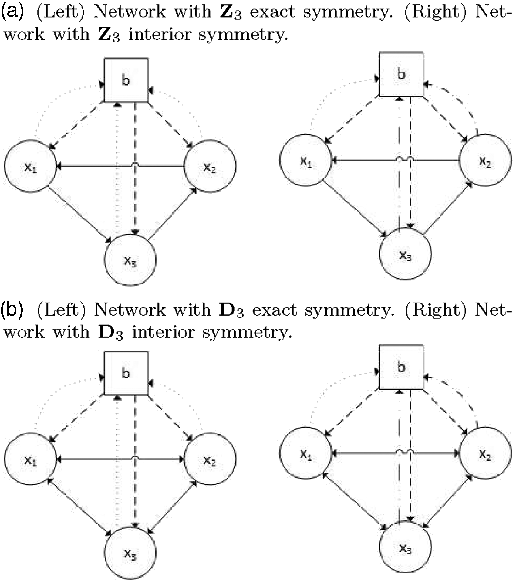

In Section 2, we briefly review the theory of coupled cell networks and bifurcation theory for symmetric dynamical systems. In Section 3, we simulate the coupled cell systems associated with the networks in Figure 1. In Section 4, we conclude this work and unveil future research directions.

2. Coupled cells and symmetry

A network of cells may be drawn as a directed graph, whose nodes represent the cells and whose edges distinguish couplings between them. Cells and arrows may be classified according to certain types (Stewart et al., 2003; Golubitsky et al., 2005). Cells of the same type have the same internal dynamics, and arrows with the same label identify equal couplings. Each cell is a dynamical system. The input set of a cell is the set of edges directed to that cell. Input isomorphisms are label-preserving bijections between input sets of cells. These isomorphisms obey the local symmetries of the network. These local symmetries have the structure of a groupoid. The latter means that they have the properties of a group, even though some products of elements may not always be defined. Figure 1 depicts four examples of coupled cell networks, where the nodes are drawn as circles (cells in the rings) and squares (‘buffer’ cell). In Figure 1 (left) there are three different types of couplings in the two networks, whereas in Figure 1 (right) there are five different types of couplings in the two networks.

Coupled cell systems are dynamical systems consistent with the architecture or topology of the graph representing the network. Each cell c_j of the network has an internal phase space P_j: here we always assume that P_j is a Euclidean space R ^k . The total phase space of the network is the direct product of internal phases spaces of each cell, $P = Π_{i = 1}^{n} 1 mu P_{i} .$ Coordinates on P_j are denoted by x_j and coordinates on P are denoted by $(x_{1}, \dots, x_{n})$ . The state of the system at time t is $(x_{1} (t), \dots, x_{n} (t))$ , where x_j(t) ∈ P_j is the state of cell c_j at time t.

A vector field f on P is called admissible, for a given network, if it satisfies the two following conditions (Golubitsky and Stewart, 2006):

Domain condition: each component f_j corresponding to a cell c_j is a function only of the variables associated with the cells c_k that have edges directed to c_j;

Pull-back condition: two components f_j and f_k corresponding to cells c_j and c_k with isomorphic input sets are identical up to a suitable permutation of the relevant variables.

In this work, we consider an important class of networks, namely, networks that possess a group of symmetries, either exact or ‘interior’ symmetry. A symmetry of a coupled cell system is the group of permutations of the cells (and arrows) that preserves the network structure (including cell labels and arrow labels) and its action on P is by permutation of cell coordinates. It is thus a transformation of the phase space that sends solutions to solutions. The networks in Figure 1(a) are examples of networks with Z₃ symmetry. Moreover, the networks in Figure 1(b) are examples of networks with D₃ symmetry.

The notion of ‘interior’ symmetry was introduced by Golubitsky et al. (2004b), and it generalizes the usual definition of symmetry. The network in Figure 1(a), right, is a network with interior Z₃ symmetry group. Moreover, note that if we delete the arrows directed from the rings to the ‘buffer’ cell, then we obtain the schematic diagram on the left of Figure 1(a), which is an example of a network with Z₃ exact symmetry. In this case, there is a group of permutations that acts in a subset of cells (but not on the entire set of cells) and partially preserves the network structure (cell labels and edge labels). The same reasoning applies for the networks in Figure 1(b). On the left, the network has D₃ exact symmetry group. On the right, the network has D₃ ‘interior’ symmetry group.

2.1. Bifurcations in coupled cell systems

A bifurcation of a coupled cell system is associated with a change in the qualitative behavior of that system, when a parameter is varied. Generically, there are two local bifurcations from a synchronous equilibrium: the synchrony-breaking bifurcation and the synchrony-preserving bifurcations. The first bifurcation is characterized by a loss of symmetry of the solution when the bifurcation occurs. These bifurcations may be viewed as generalizations of symmetry-breaking bifurcations in symmetric coupled cell systems. The equivariant branching lemma proves the existence of certain branches of symmetry-breaking steady states (Golubitsky et al., 1988). The equivariant Hopf theorem guarantees the existence of families of small-amplitude periodic solutions bifurcating from the origin (Golubitsky et al., 1988). Generalizations of the equivariant branching lemma and the equivariant Hopf theorem for coupled cell systems with interior symmetries are given by Golubitsky et al. (2004b) and Antoneli et al. (2007).

We can produce a list of all spatio-temporal patterns satisfying the conditions of the above results and that are expected to occur when one of the coupled cell systems associated with the networks of Figure 1 undergoes an (interior) symmetry-breaking Hopf bifurcation.

Returning to the example with Z₃ (interior) symmetry, we conclude there is only one (interior) solution with symmetry type ${\tilde{Z}}_{3}$ . These solutions are also called rotating waves in the case of exact symmetry and approximate rotating waves in the case of interior symmetry (Golubitsky et al., 1988; Antoneli et al., 2010).

Considering the networks in Figure 1(a), when the symmetry is exact the periodic solution of type ${\tilde{Z}}_{3}$ is such that its components corresponding to the cells in the 3-ring are periodic and have the same waveform but they are 1/3 out of phase. When the symmetry is only interior it is almost the same as in the case when it is exact, with the exception that the ‘buffer’ cell that stayed in equilibrium is now oscillating as well.

In the second case (Figure 1(b)), there are three solutions corresponding to symmetry types ${\tilde{Z}}_{3}$ , Z₂ and ${\tilde{Z}}_{2}$ (Golubitsky et al., 1988). The periodic solution corresponding to the first type is called a discrete rotating wave and has spatio-temporal symmetry generated by a rotation. The periodic solution corresponding to the second type has purely spatial symmetry generated by a reflection. The periodic solution corresponding to the third type has spatio-temporal symmetry generated by a reflection. In this work, we only observe (approximate) rotating waves, which have the same form as in the case of unidirectional rings, for the networks with D₃ (interior) symmetry in Figure 1(b).

3. Numerical simulations

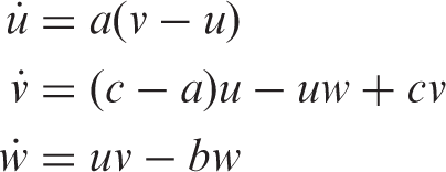
The coupled cell systems associated with the networks depicted in Figure 1 are simulated. We use XPPAUT (Ermentrout, 2006) and MATLAB (http://www.mathworks.com) to numerically compute the relevant states. We consider the Chen oscillator as the internal dynamics of each cell in the 3-ring and a unidimensional phase space for the ‘buffer’ cell. The total phase space is thus ten-dimensional. The dynamics of a singular ring cell are given by (Chen and Ueta, 1999; Lu et al., 2002)

\overset{\cdot}{u} = a (v - u) \overset{\cdot}{v} = (c - a) u - uw + cv \overset{\cdot}{w} = uv - bw

(1)

where a = 35, b = 3 and c are real parameters. The unidimensional dynamics of the ‘buffer’ cell are given by (Antoneli et al., 2008; Golubitsky et al., 2004a)

f (u) = - μ u - \frac{1}{10} u^{2} - u^{3}

(2)

where μ = −1.0 is a real parameter.

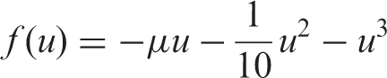
The coupled cell system of equations associated with the networks in Figure 1 is given by

{\overset{\cdot}{x}}_{j} = g (x_{j}) + c_{1} (x_{j} - x_{j + 1}) + c_{2} (x_{j} - x_{j + 2}) + db, j = 1, \dots, 3 \overset{\cdot}{b} = f (b) + λ (e_{1} x_{1} + e_{2} x_{2} + e_{3} x_{3})

(3)

where g(u) represents the dynamics of each Chen oscillator, c₁ = −5, d = 0.2, e₁ = 0.1, e₂ = 0.2, e₃ = 0.3 and the indexing assumes

x_{4} \equiv x_{1}

. We assume that the coupling between all cells is linear and is done only in the first variable of each Chen oscillator. This choice of the coupling is related to previous work (Antoneli et al., 2007, 2008, 2010; Pinto, 2012).

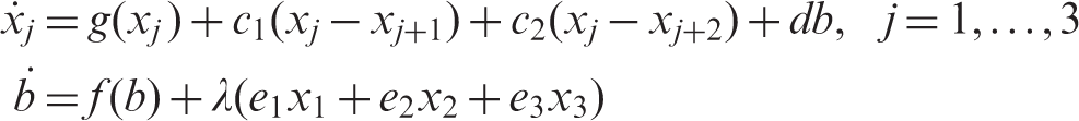
The system has exact symmetry for λ = 0 (networks in Figure 1 (right)) and ‘interior’ symmetry for λ ≠ 0 (networks in Figure 1 (left)). If c₂ = 0 then the coupled cell system is admissible for the networks in Figure 1(a) with Z₃ symmetry. If c₂ ≠ 0, then the system is admissible for the networks in Figure 1(b) with D₃ symmetry group.

3.1. Unidirectional networks: dynamics

We vary parameter c ∈ [15, 27], going from lower to higher values, and start from a steady state of the whole system.

We consider c₂ = 0: this means that we will simulate the coupled cell systems associated with the unidirectional rings (Figure 1(a)), for λ = 0 and λ ≠ 0.

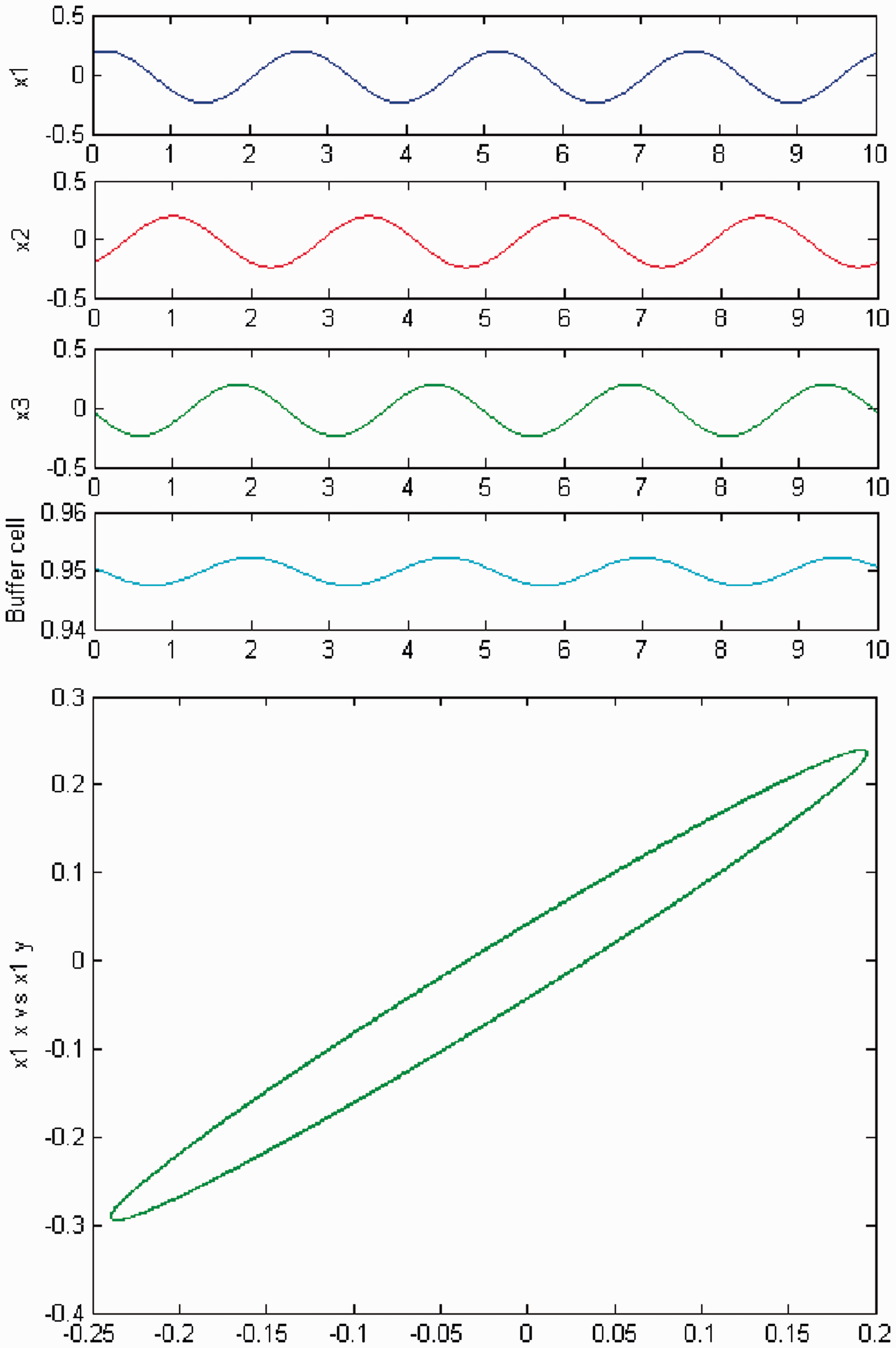
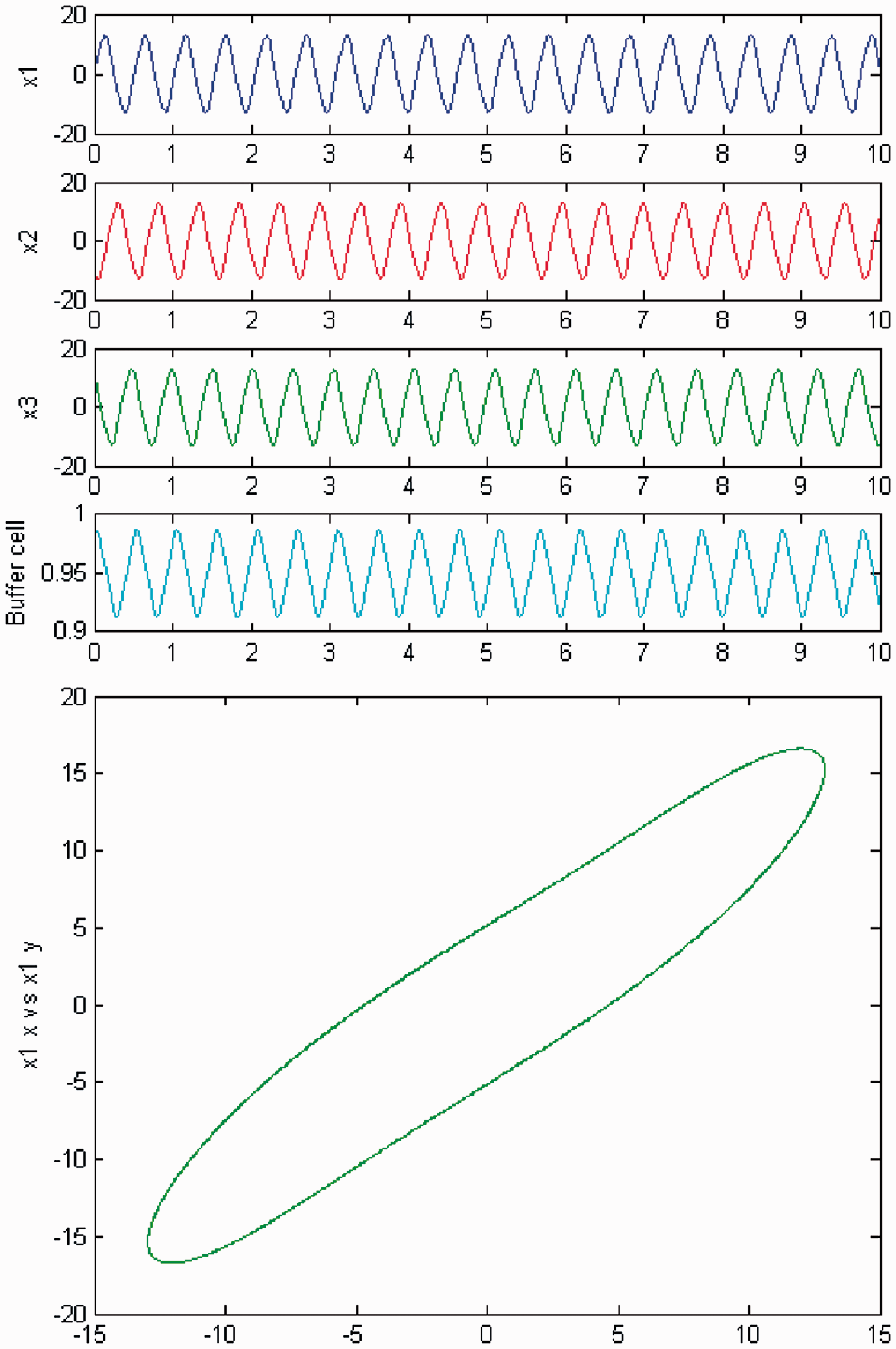
We increase c and a primary Hopf bifurcation occurs (HB1). In Figures 2 and 3, we plot (top) the time series of the solution of the coupled cell system (3), and (bottom) the phase space of the oscillator x₁ of the ring. The solution is a Z₃ rotating wave in the 3-ring for the case of exact symmetry (λ = 0), and an approximate rotating wave state in the case of interior symmetry (λ ≠ 0). The ‘buffer’ cell is in equilibrium in the case of exact symmetry and depicts a periodic state in the case of interior symmetry. The full solution is periodic in both cases.

Figure 2.

Simulation of the coupled system (3) for λ = 0 and c₂ = 0. (Top) Time series of the cells in the 3-ring and of the ‘buffer’ cell, for c = 15.59, after the first Hopf bifurcation point (HB1). The cells in the ring exhibit a Z₃ rotating wave. The ‘buffer’ cell is in equilibrium. (Bottom) Phase space of the oscillator x₁.

Figure 3.

Simulation of the coupled system (3), for λ ≠ 0 and c₂ = 0. (Top) Time series of the cells in the 3-ring and of the ‘buffer’ cell, for c = 15.59, after the first Hopf bifurcation point (HB1). The cells in the ring depict a 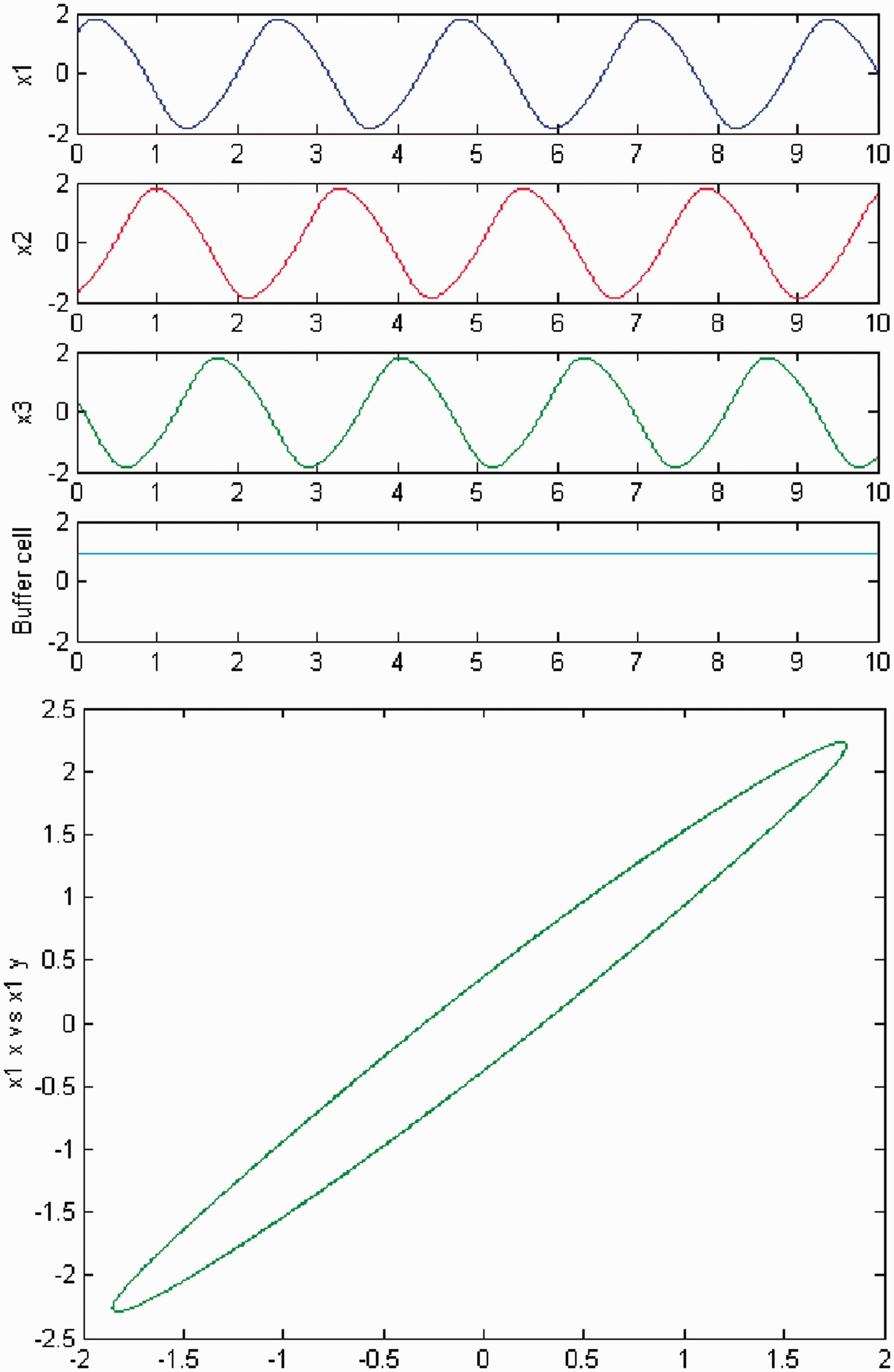Z₃ rotating wave and the ‘buffer’ cell is periodic. (Bottom) Phase space of the oscillator x₁.

We increase c again, and a second Hopf bifurcation occurs (HB2). In Figures 4 and 5, we plot (top) the time series of the solution of the coupled cell system (3), and (bottom) the phase space of the oscillator x₁ of the 3-ring. The solution is a Z₃ rotating wave in the 3-ring in the case of exact symmetry and an approximate rotating wave in the case of interior symmetry. We observe that the wave amplitude increases and the period decreases. The full solution is periodic. Note that these solutions reveal characteristics of relaxation oscillations (Krupa and Szmolyan, 2001) (more on this in Section 3.3).

Figure 4.

Simulation of the coupled system (3) for λ = 0 and c₂ = 0. (Top) Time series of the cells in the 3-ring and of the ‘buffer’ cell, for c = 19.54, after the second Hopf bifurcation point (HB2). The cells in the 3-ring exhibit a Z₃ rotating wave. The ‘buffer’ cell is in equilibrium. (Bottom) Phase space of the oscillator x₁.

Figure 5.

Simulation of the coupled system (3) for λ ≠ 0 and c₂ = 0. (Top) Time series of the cells in the 3-ring and of the ‘buffer’ cell, for c = 19.54, after the second Hopf bifurcation point (HB2). The cells in the 3-ring show a 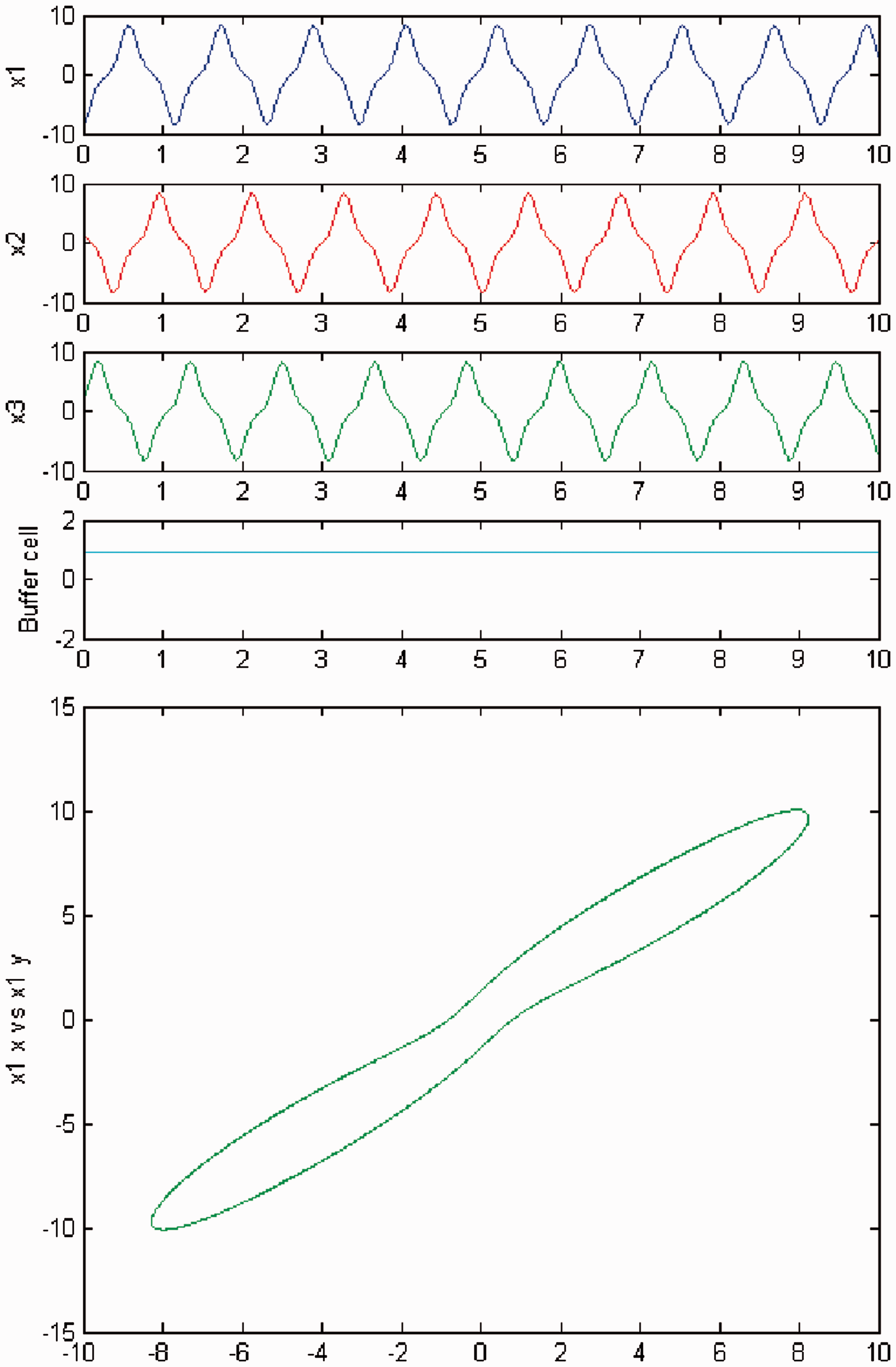Z₃ rotating wave and the ‘buffer’ cell depicts periodic motion. (Bottom) Phase space of the oscillator x₁.

We increase parameter c again and a third Hopf bifurcation occurs (HB3). In Figures 6 and 7, we plot (top) the time series of the solution of the coupled cell system (3), and (bottom) the phase space of the oscillator x₁ of the 3-ring. The solution is a Z₃ rotating wave in the ring. The ‘buffer’ cell is in a steady state in the case of exact symmetry, and in a periodic state in the case of ‘interior’ symmetry. The full solution is periodic. The period of the solutions decreases slightly.

Figure 6.

Simulation of the coupled system (3) for λ = 0 and c₂ = 0. (Top) Time series of the cells in the 3-ring and of the ‘buffer’ cell, for c = 20.09, after the third Hopf bifurcation point (HB3). The cells in the 3-ring exhibit a Z₃ rotating wave. The ‘buffer’ cell is in equilibrium. (Bottom) Phase space of the oscillator x₁.

Figure 7.

Simulation of the coupled system (3) for λ ≠ 0 and c₂ = 0. (Top) Time series of the cells in the 3-ring and of the ‘buffer’ cell, for c = 20.09, after the third Hopf bifurcation point (HB3). The cells in the 3-ring exhibit a Z₃ rotating wave. The ‘buffer’ cell is in a periodic state. (Bottom) Phase space of the oscillator x₁.

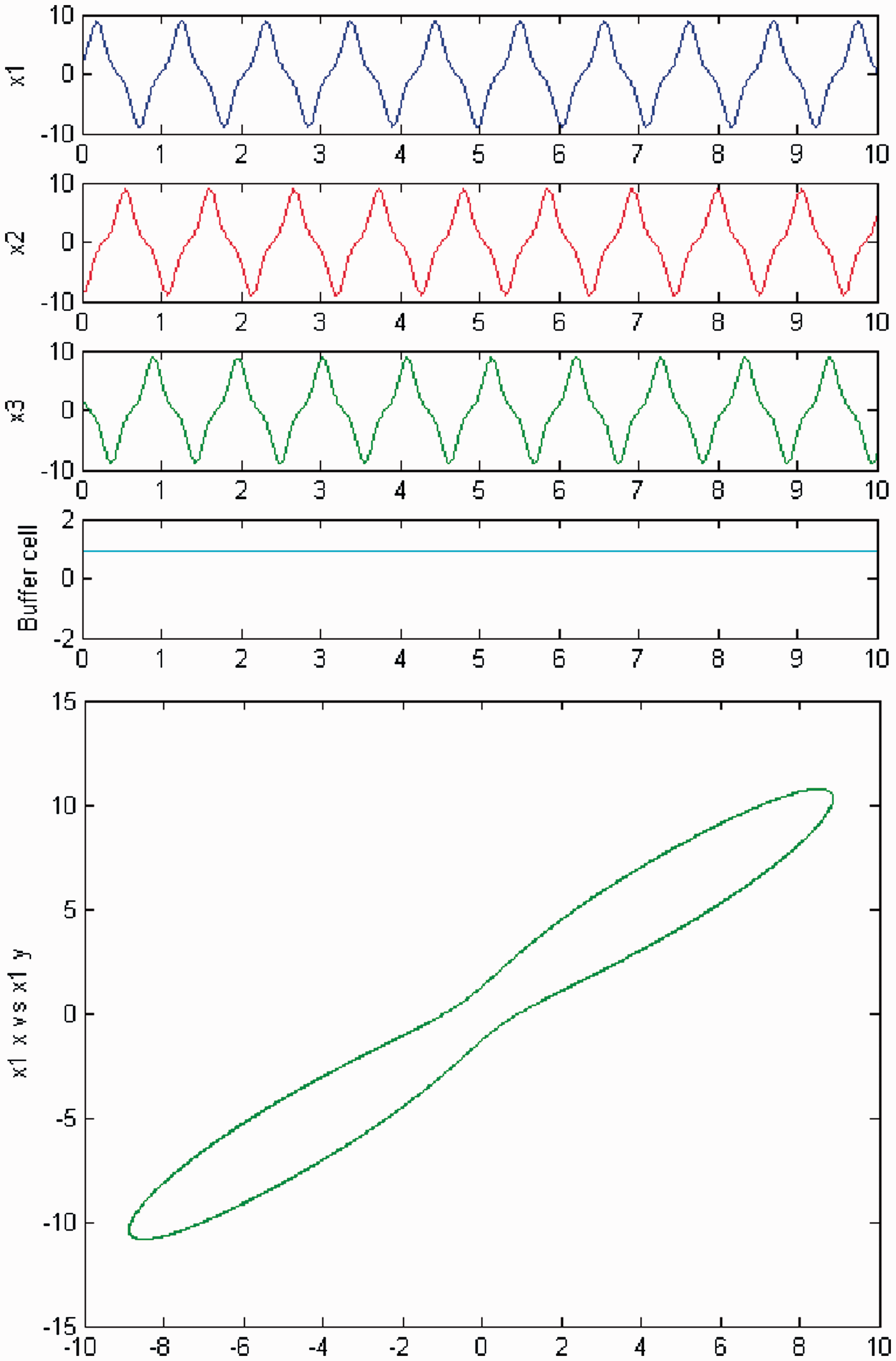
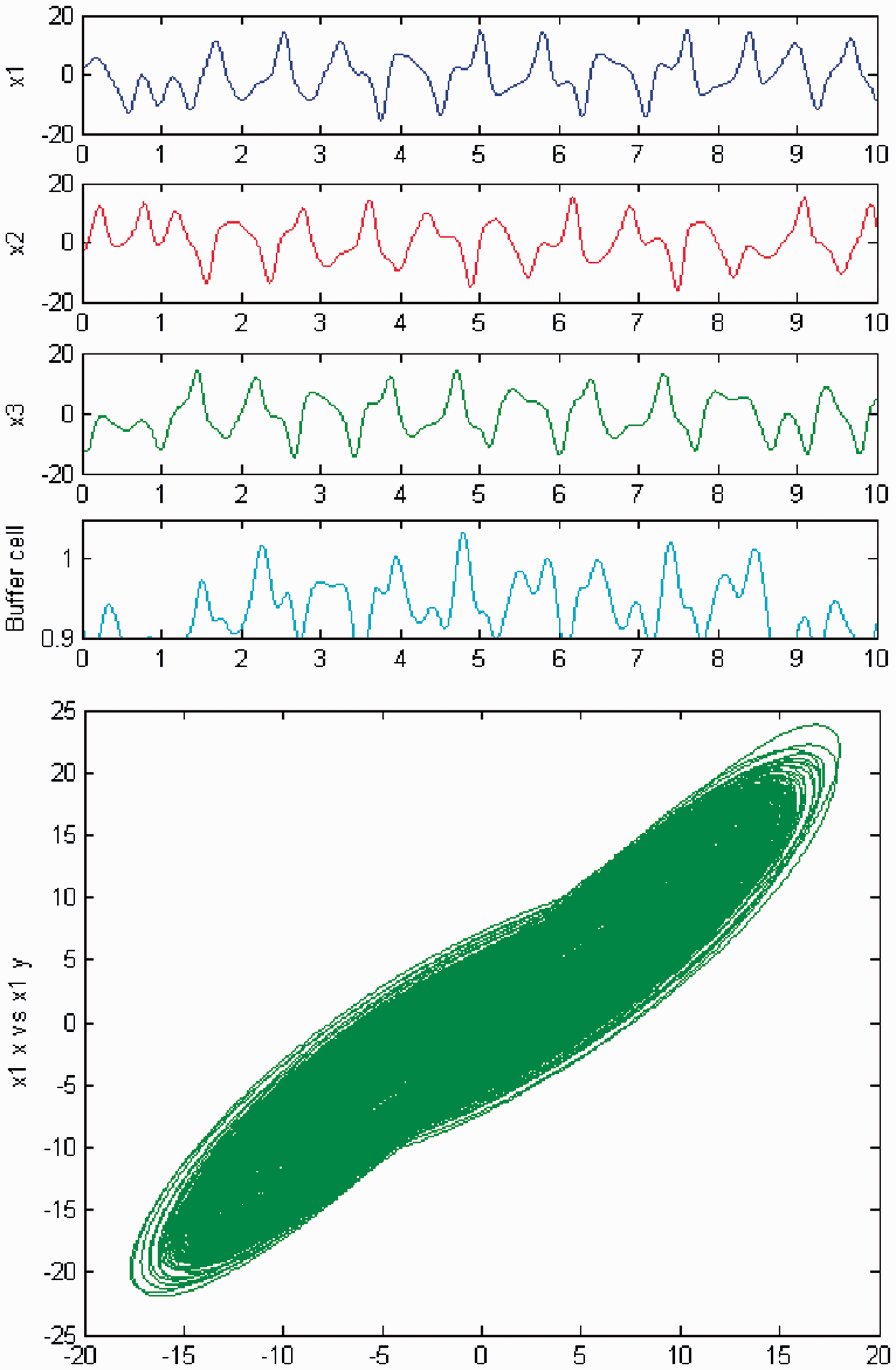
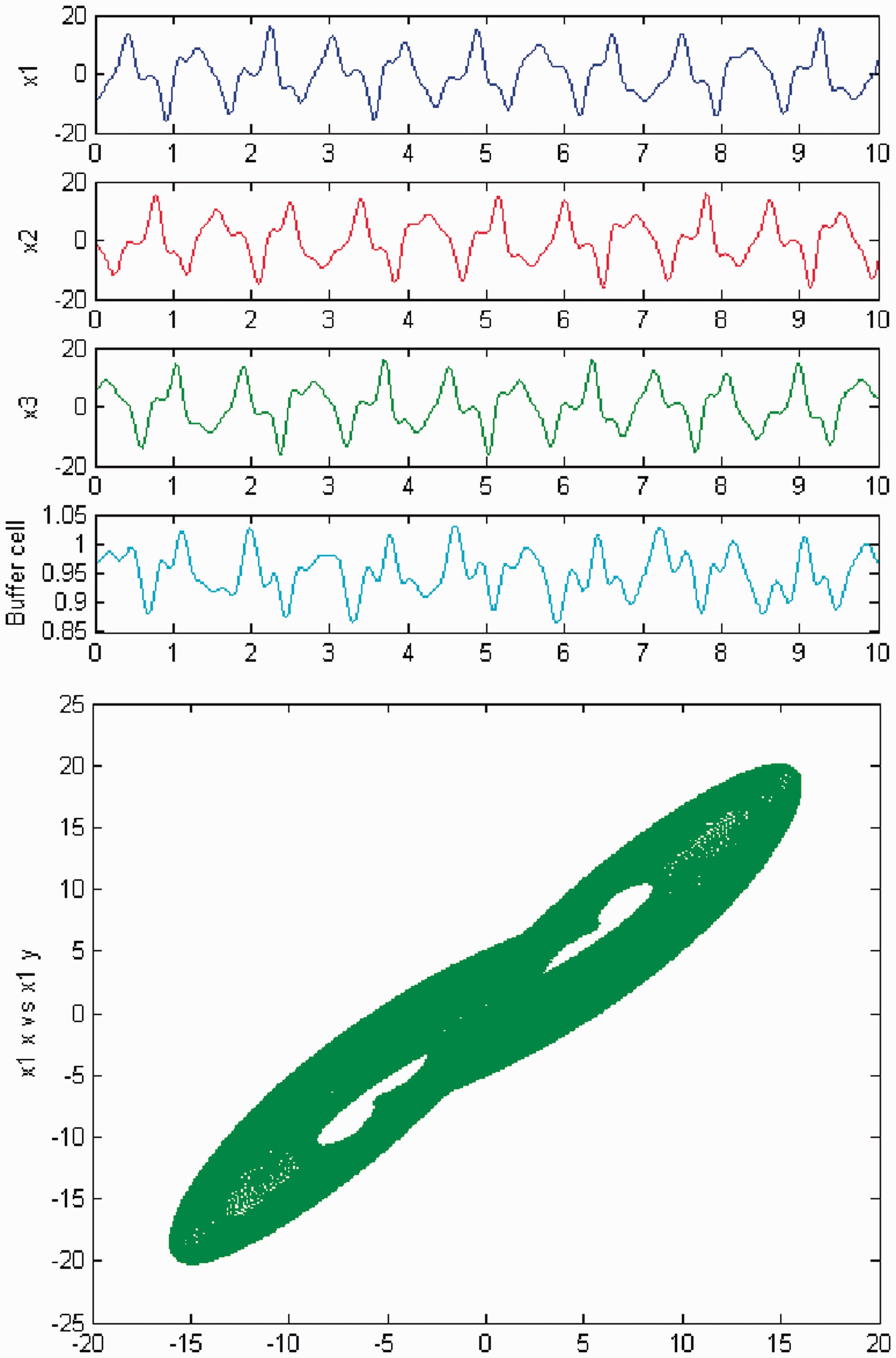
Increasing parameter c further away from the third Hopf point, a change in the qualitative behavior of the system (3) is observed, for the cases of exact (Figure 8) and ‘interior’ (Figure 9) symmetry. Namely, the cells in the 3-ring appear to show quasiperiodic motion. The ‘buffer’ cell is in equilibrium in the case of exact symmetry and appears to be quasiperiodic in the case of ‘interior’ symmetry. The full solution is quasiperiodic.

Figure 8.

Simulation of the coupled system (3) for λ = 0 and c₂ = 0. (Top) Time series of the cells in the 3-ring and of the ‘buffer’ cell, for c = 22.6, further away from the third Hopf bifurcation point (HB3). The cells in the 3-ring depict quasiperiodic motion and the ‘buffer’ cell is in a steady state. (Bottom) Phase space of the oscillator x₁.

Figure 9.

Simulation of the coupled system (3) for λ ≠ 0 and c₂ = 0. (Top) Time series of the cells in the 3-ring and of the ‘buffer’ cell, for c = 22.6, further away from the third Hopf bifurcation point (HB3). All cells depict quasiperiodic motion. (Bottom) Phase space of the oscillator x₁.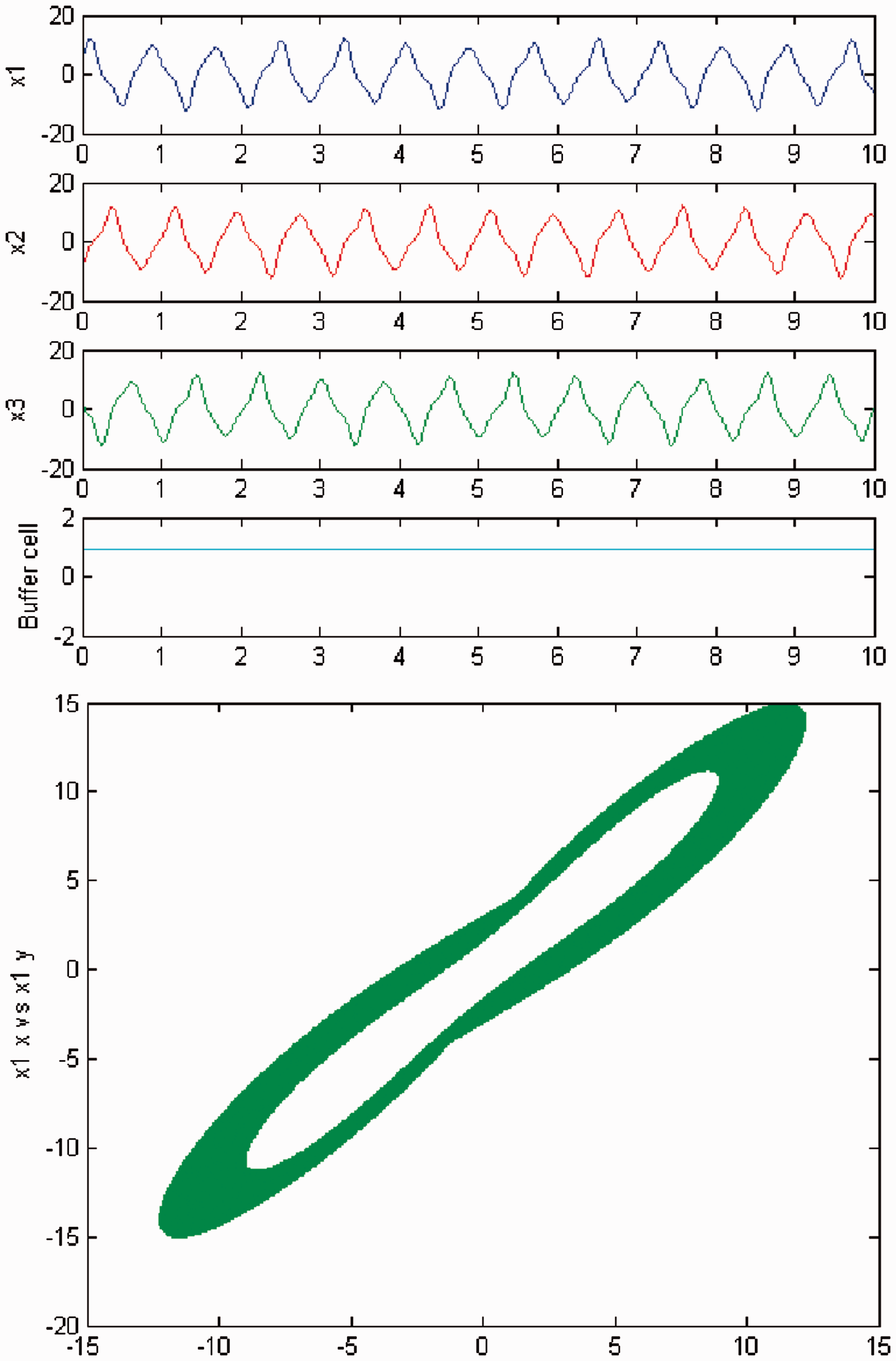

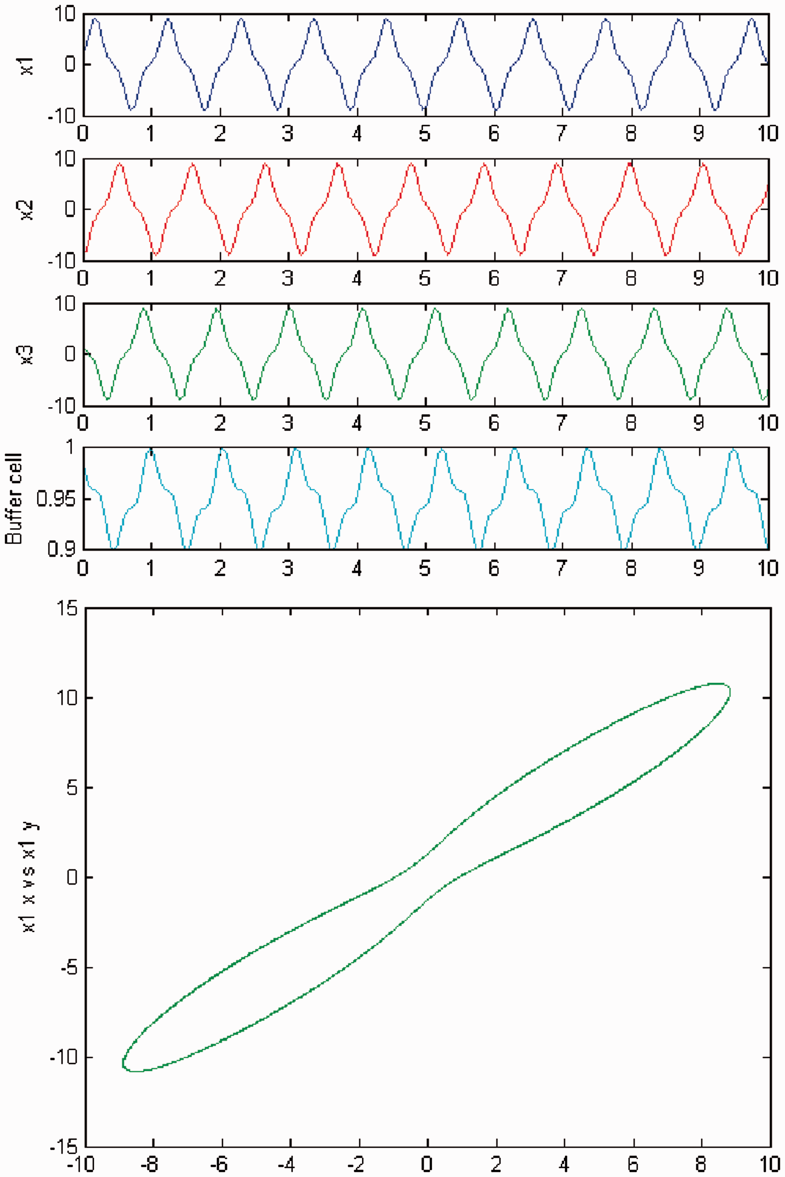
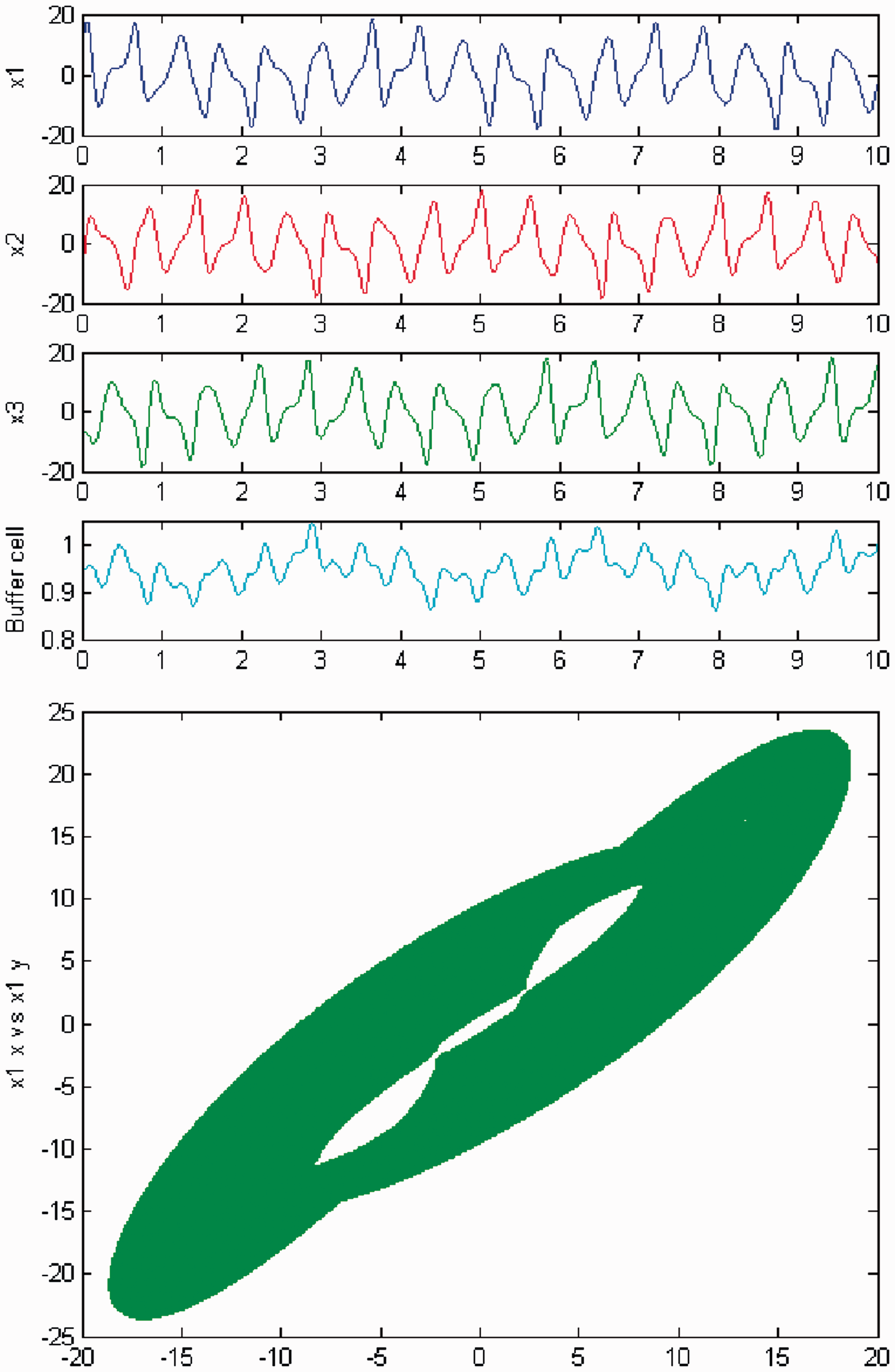
We continue to increase c. The cells in the 3-ring depict a quasiperiodic state (Figures 10 and 11), looking more ‘complex’ than the one in Figures 8 and 9. The ‘buffer’ cell is in a steady state for λ = 0 and shows quasiperiodic motion for λ ≠ 0. The full solution is quasiperiodic.

Figure 10.

Simulation of the coupled system (3) for λ = 0 and c₂ = 0. (Top) Time series of the cells in the 3-ring and of the ‘buffer’ cell, for c = 23. The cells in the ring exhibit quasiperiodic motion. The ‘buffer’ cell is in equilibrium. (Bottom) Phase space of the oscillator x₁.

Figure 11.

Simulation of the coupled system (3) for λ ≠ 0 and c₂ = 0. (Top) Time series of the cells in the 3-ring and of the ‘buffer’ cell, for c = 23. All cells show quasiperiodic motion. (Bottom) Phase space of the oscillator x₁.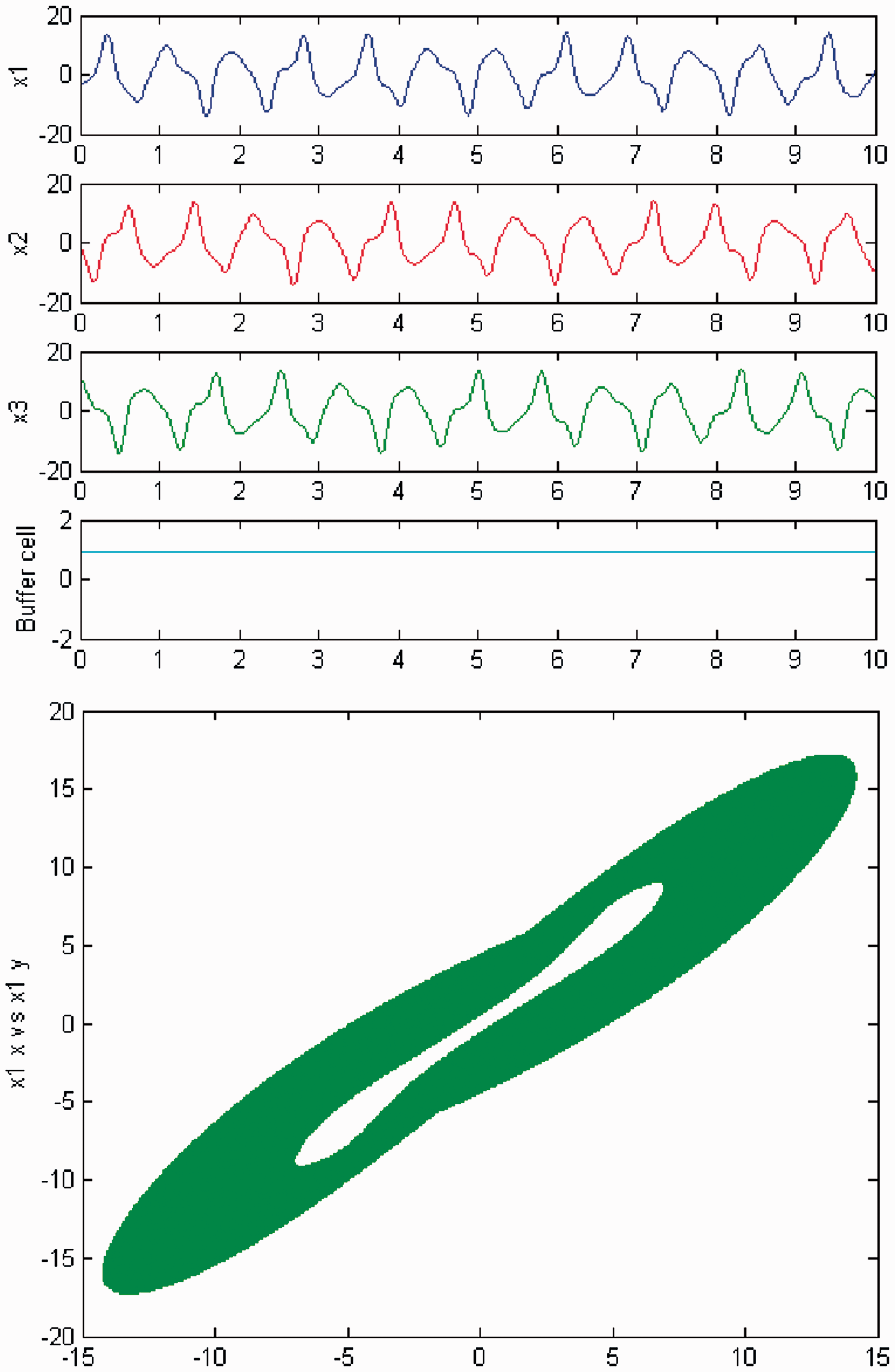

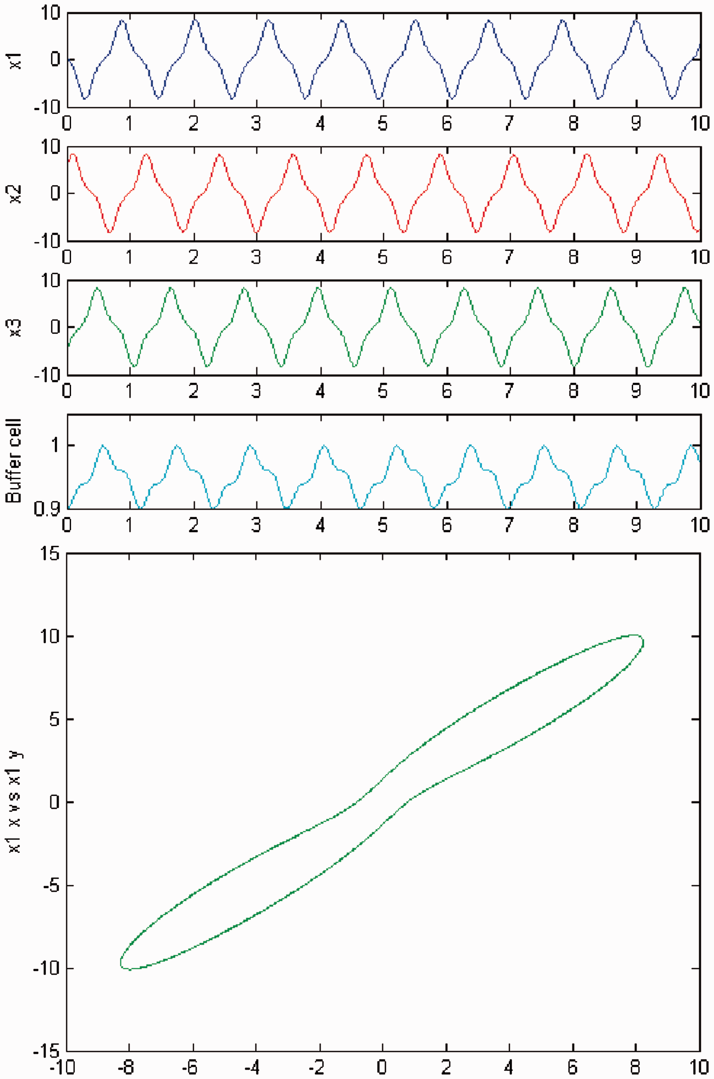
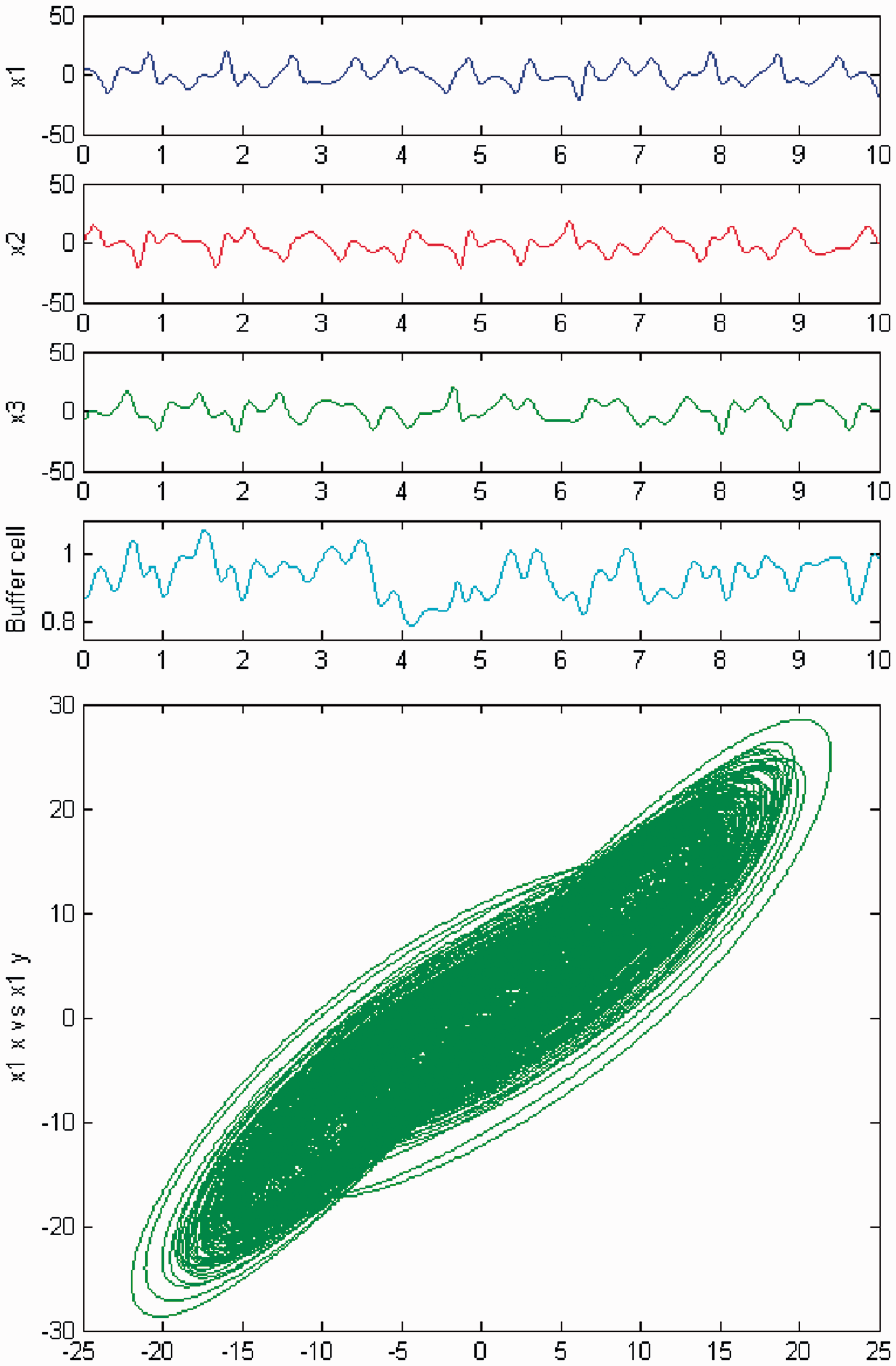
We persist in increasing the parameter c, and a new qualitative change in the behavior of the coupled cell system (3) is visible. Cells in the 3-ring show chaotic motion (see Figures 12 and 13). The ‘buffer’ cell is in a steady state in the case of exact symmetry and in a chaotic state for the case of ‘interior’ symmetry.

Figure 12.

Simulation of the coupled system (3) for λ = 0 and c₂ = 0. (Top) Time series of the cells in the 3-ring and of the ‘buffer’ cell, for c = 23.4. The cells in the 3-ring exhibit chaotic motion. The ‘buffer’ cell is in a steady state. (Bottom) Phase space of the oscillator x₁.

Figure 13.

Simulation of the coupled system (3) for λ ≠ 0 and c₂ = 0. (Top) Time series of the cells in the 3-ring and of the ‘buffer’ cell, for c = 23.4. All cells in the network depict chaotic motion. (Bottom) Phase space of the oscillator x₁.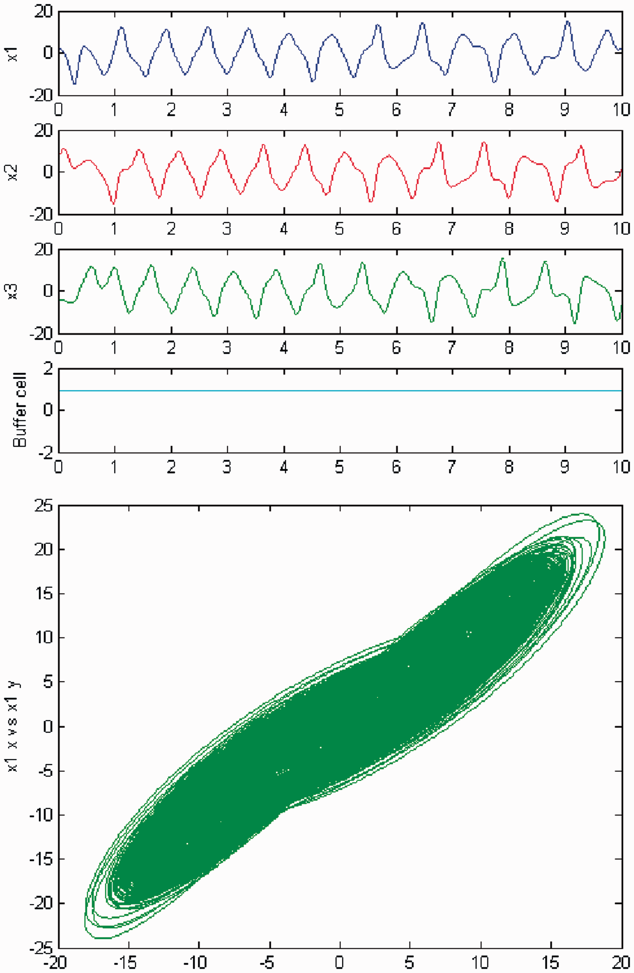

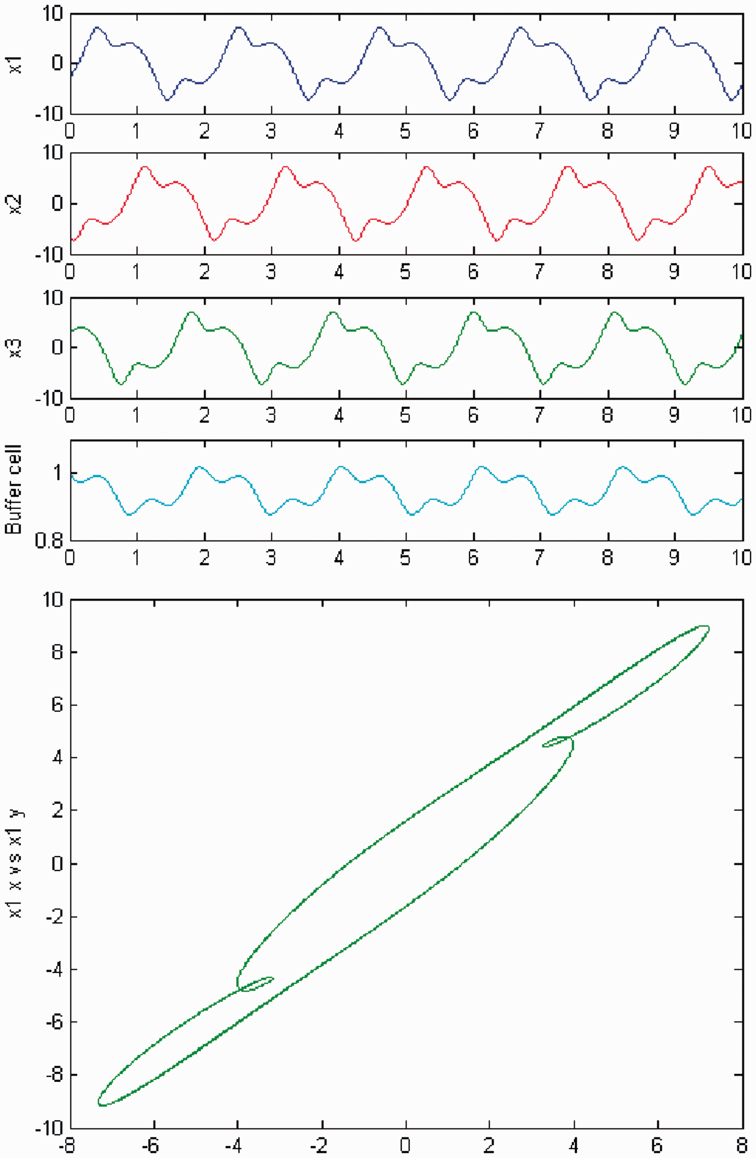
Incrementing c again, another change occurs in the dynamical behavior of the cells of the networks in Figure 1(a). The cells in the 3-ring now depict quasiperiodic motion again (Figures 14 and 15). The ‘buffer’ cell is in equilibrium for λ = 0 and in a quasiperiodic state for λ ≠ 0. The full solution is quasiperiodic.

Figure 14.

Simulation of the coupled system (3) for λ = 0 and c₂ = 0. (Top) Time series of the cells in the 3-ring and of the ‘buffer’ cell, for c = 25.6. The cells in the 3-ring show quasiperiodic motion. The ‘buffer’ cell is in equilibrium. (Bottom) Phase space of the oscillator x₁.

Figure 15.

Simulation of the coupled system (3) for λ ≠ 0 and c₂ = 0. (Top) Time series of the cells in the 3-ring and of the ‘buffer’ cell, for c = 25.6. All cells in the network show quasiperiodic motion. (Bottom) Phase space of the oscillator x₁.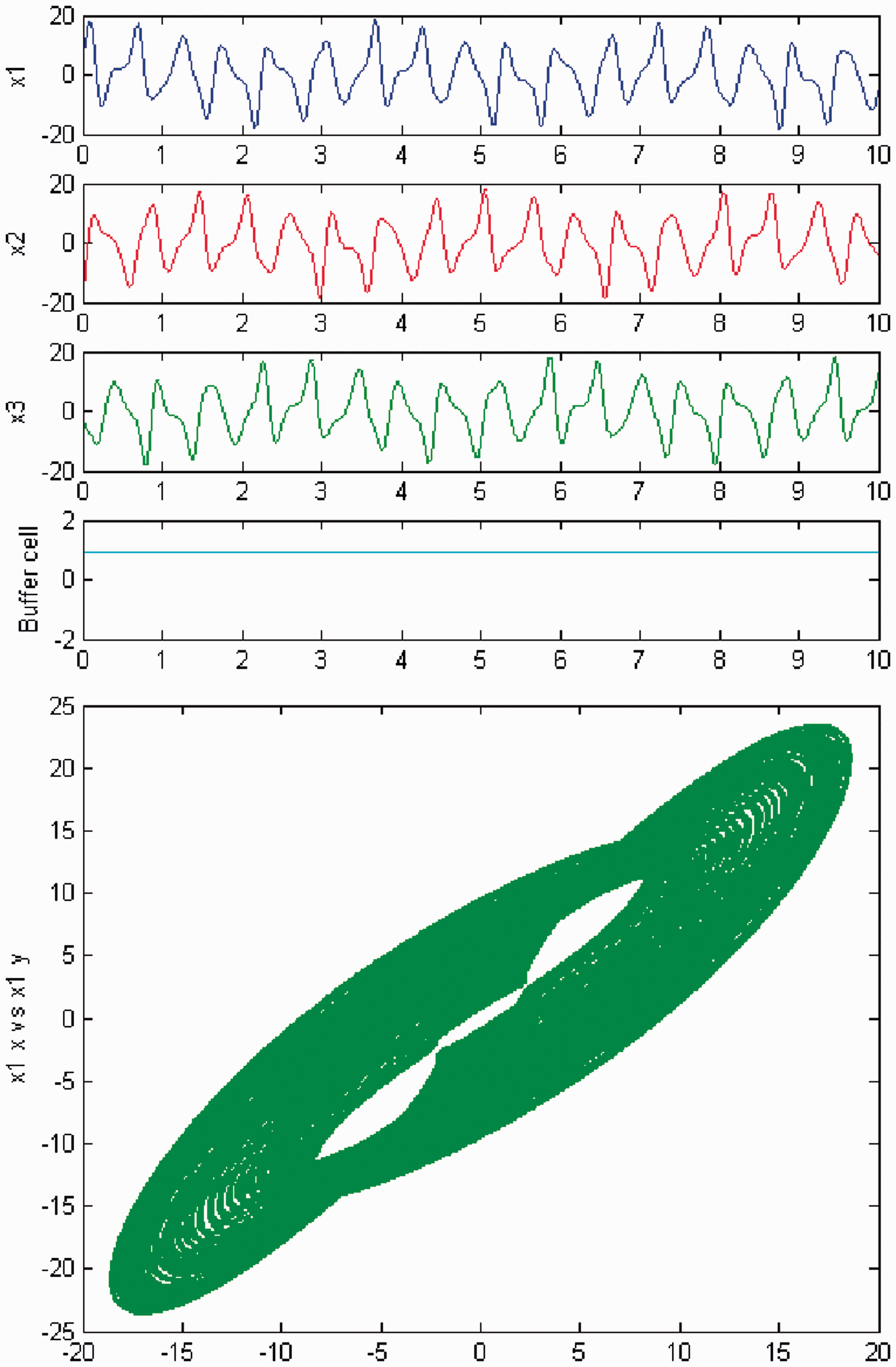

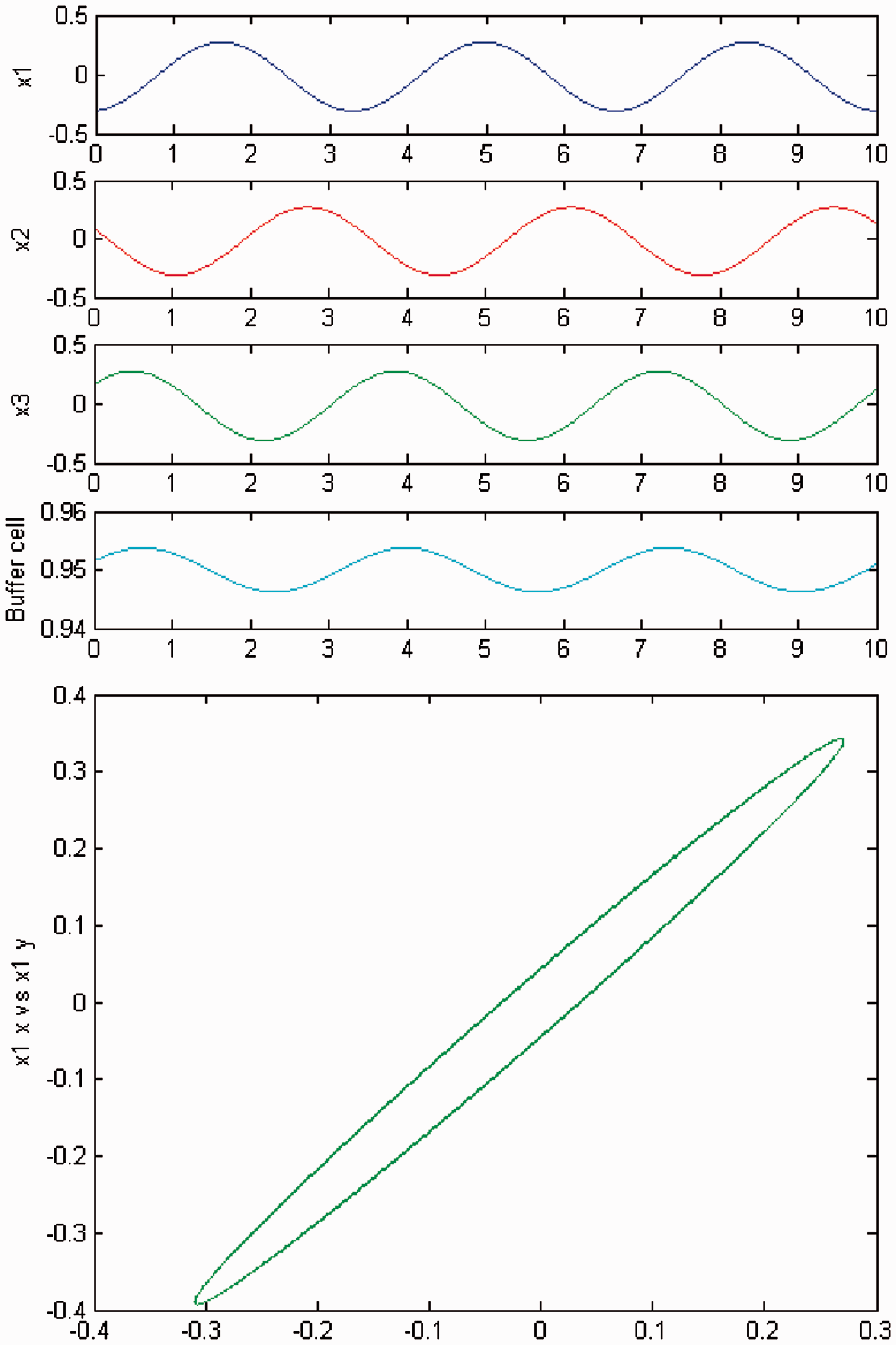
The quasiperiodic behavior disappears as c is increased once again. The coupled cell system returns to a periodic state, where the cells in the 3-ring depict a Z₃ rotating wave state (Figures 16 and 17). The ‘buffer’ cell is in equilibrium for λ = 0 and is periodic for λ ≠ 0. The full solution is periodic.

Figure 16.

Simulation of the coupled system (3) for λ = 0 and c₂ = 0. (Top) Time series of the cells in the 3-ring and of the ‘buffer’ cell, for c = 27. The cells in the ring depict a Z₃ rotating wave. The ‘buffer’ cell is in equilibrium. (Bottom) Phase space of the oscillator x₁.

Figure 17.

Simulation of the coupled system (3) for λ ≠ 0 and c₂ = 0. (Top) Time series of the cells in the 3-ring and of the ‘buffer’ cell, for c = 27. The cells in the ring exhibit a 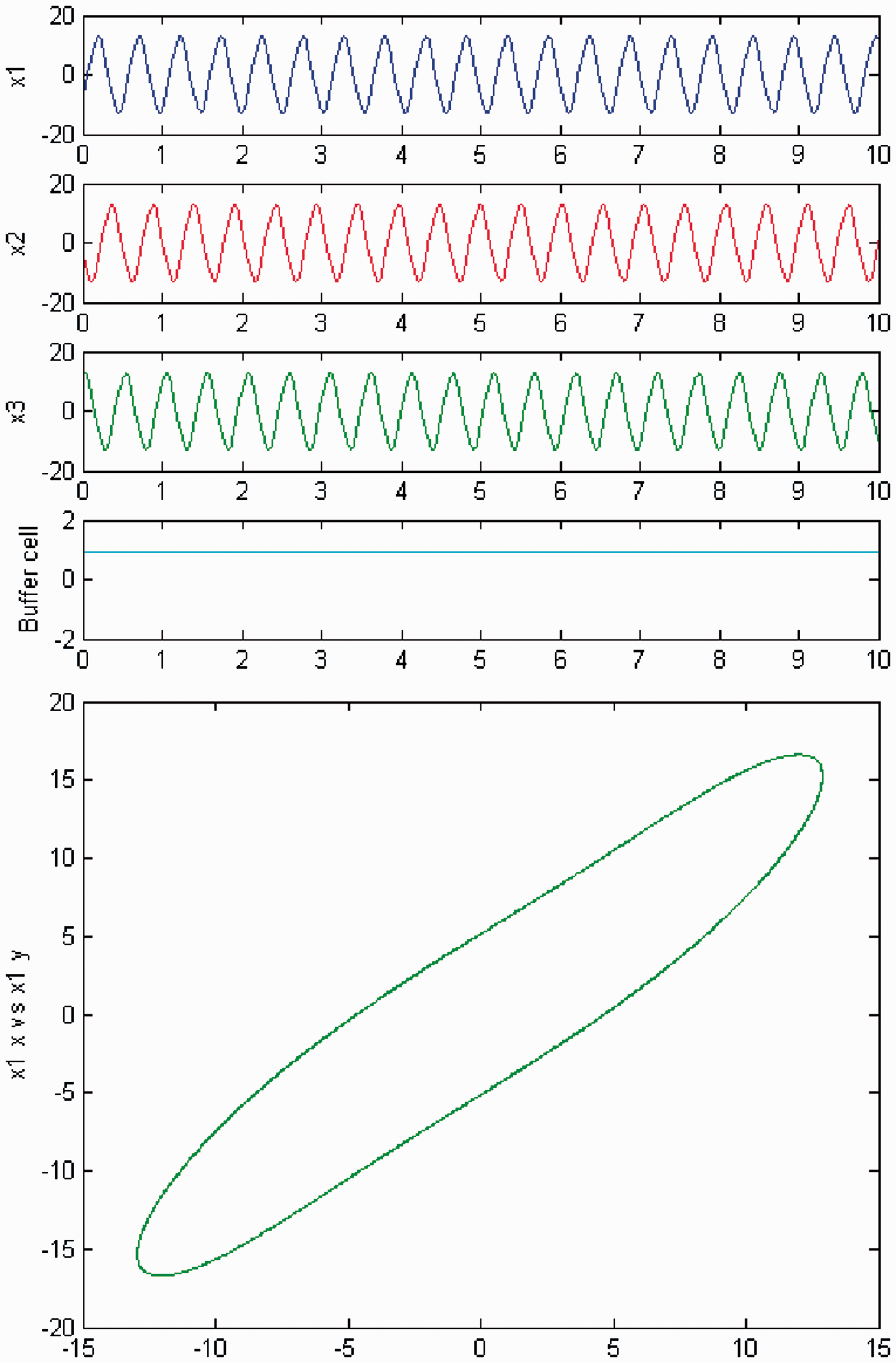Z₃ rotating wave. The ‘buffer’ cell is periodic. (Bottom) Phase space of the oscillator x₁.

3.2. Bidirectional networks: dynamics

We now simulate the networks in Figure 1(b). We vary parameter c ∈ [15, 29], going from lower to higher values, and start from a steady state of the whole system. We now set c₂ = −1, and consider the cases λ = 0 and λ ≠ 0.

We increase the parameter c, starting at c = 15, and a first Hopf bifurcation (HB1) occurs at c = 15.39, from the full equilibrium of the system. The cells in the 3-ring depict a Z₃ rotating wave. The ‘buffer’ cell is in equilibrium for the case of exact symmetry (Figure 18) and in a periodic state in the case of ‘interior’ symmetry (Figure 19).

Figure 18.

Simulation of the coupled system (3) for λ = 0 and c₂ ≠ 0. (Top) Time series of the cells in the 3-ring and of the ‘buffer’ cell, for c = 15.39, after the first Hopf bifurcation point (HB1). The cells in the ring exhibit a Z₃ rotating wave. The ‘buffer’ cell is in equilibrium. (Bottom) Phase space of the oscillator x₁.

Figure 19.

Simulation of the coupled system (3), for λ ≠ 0 and c₂ ≠ 0. (Top) Time series of the cells in the 3-ring and of the ‘buffer’ cell, for c = 15.39, after the first Hopf bifurcation point (HB1). The cells in the ring exhibit a Z₃ rotating wave and the ‘buffer’ cell is periodic. (Bottom) Phase space of the oscillator x₁.

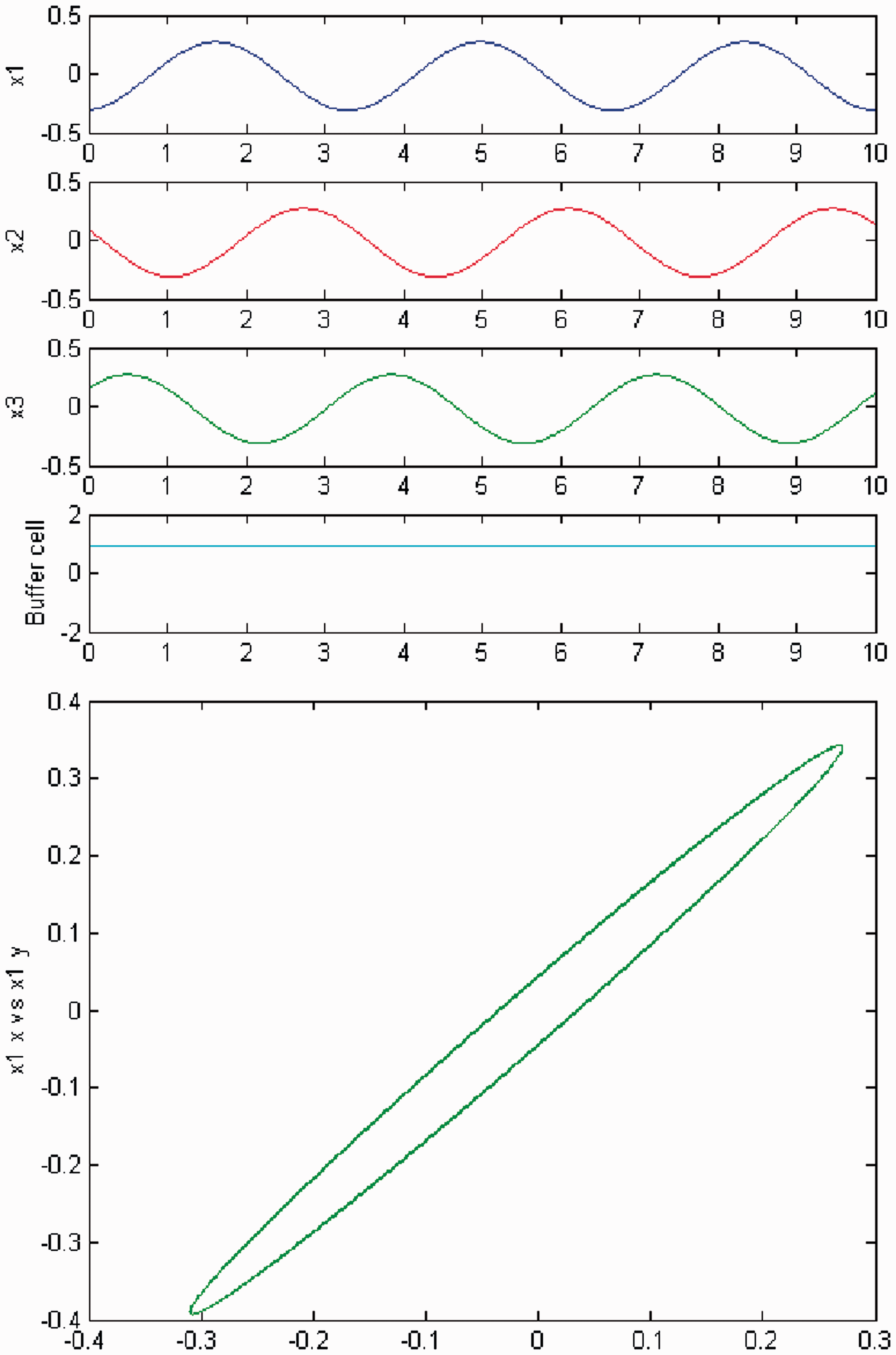
We increase c again, and a second Hopf bifurcation occurs (HB2). In Figures 20 and 21, we plot (top) the time series of the solution of the coupled cell system (3), and (bottom) the phase space of the oscillator x₁ of the 3-ring. The solution is a Z₃ rotating wave in the 3-ring in the case of exact symmetry and an approximate rotating wave in the case of ‘interior’ symmetry. We observe that the wave amplitude increases and the period decreases. The full solution is periodic. We note the appearance of relaxation oscillations (Krupa and Szmolyan, 2001) (more on this in Section 3.3).

Figure 20.

Simulation of the coupled system (3) for λ = 0 and c₂ ≠ 0. (Top) Time series of the cells in the 3-ring and of the ‘buffer’ cell, for c = 19.03, after the second Hopf bifurcation point (HB2). The cells in the 3-ring exhibit a Z₃ rotating wave. The ‘buffer’ cell is in equilibrium. (Bottom) Phase space of the oscillator x₁.

Figure 21.

Simulation of the coupled system (3) for λ ≠ 0 and c₂ ≠ 0. (Top) Time series of the cells in the 3-ring and of the ‘buffer’ cell, for c = 19.03, after the second Hopf bifurcation point (HB2). The cells in the 3-ring exhibit a Z₃ rotating wave and the ‘buffer’ cell depicts a periodic motion. (Bottom) Phase space of the oscillator x₁.

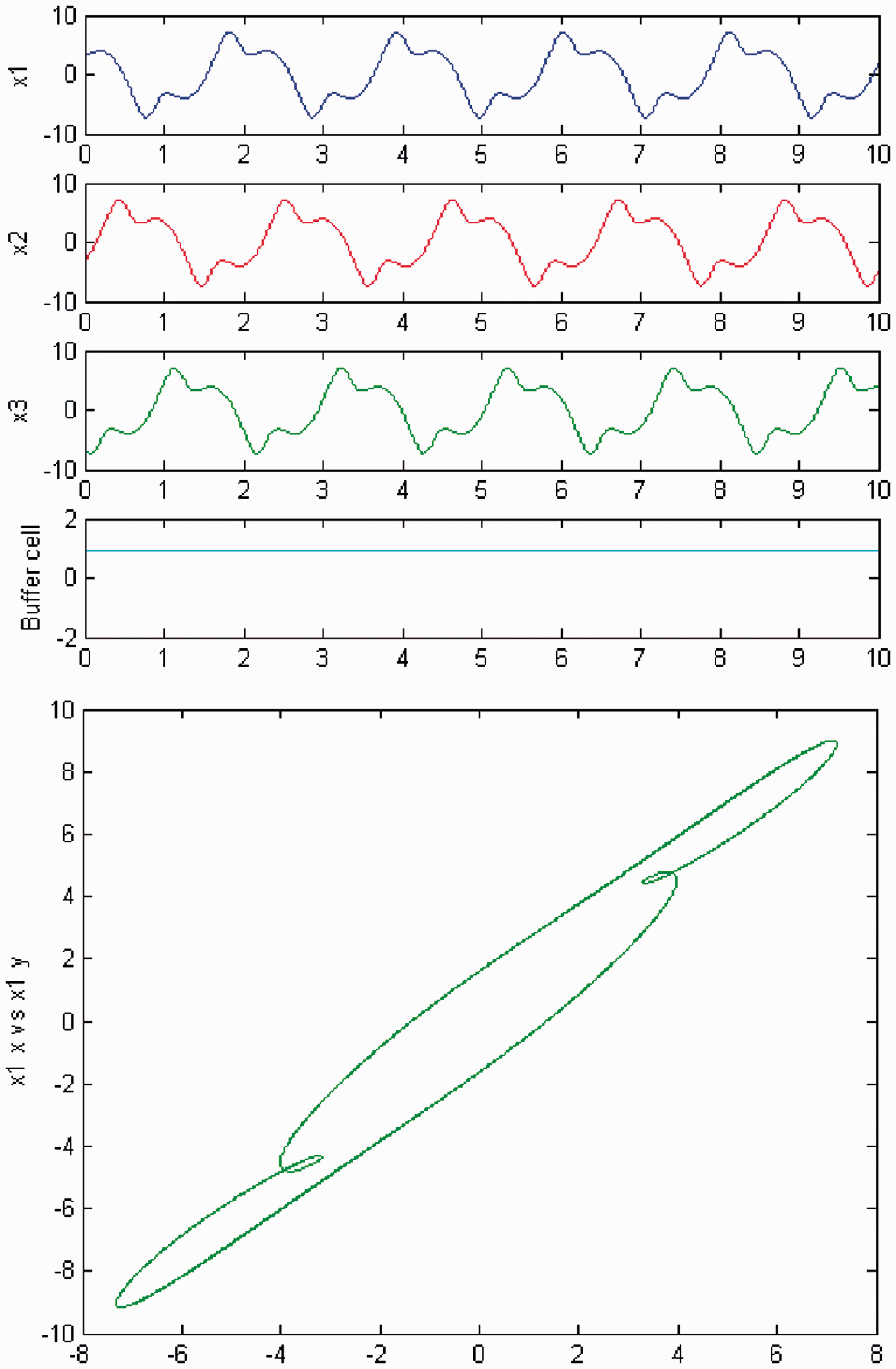
We increase parameter c again and a third Hopf bifurcation occurs (HB3). In Figures 22 and 23, we plot (top) the time series of the solution of the coupled cell system (3), and (bottom) the phase space of the oscillator x₁ of the 3-ring. The solution is a Z₃ rotating wave in the ring. The full solution is periodic.

Figure 22.

Simulation of the coupled system (3) for λ = 0 and c₂ ≠ 0. (Top) Time series of the cells in the 3-ring and of the ‘buffer’ cell, for c = 20.09, after the third Hopf bifurcation point (HB3). The cells in the 3-ring exhibit a Z₃ rotating wave. The ‘buffer’ cell is in equilibrium. (Bottom) Phase space of the oscillator x₁.

Figure 23.

Simulation of the coupled system (3) for λ ≠ 0 and c₂ ≠ 0. (Top) Time series of the cells in the 3-ring and of the ‘buffer’ cell, for c = 20.09, after the third Hopf bifurcation point (HB3). The cells in the 3-ring exhibit a Z₃ rotating wave. The ‘buffer’ cell is in a periodic state. (Bottom) Phase space of the oscillator x₁.

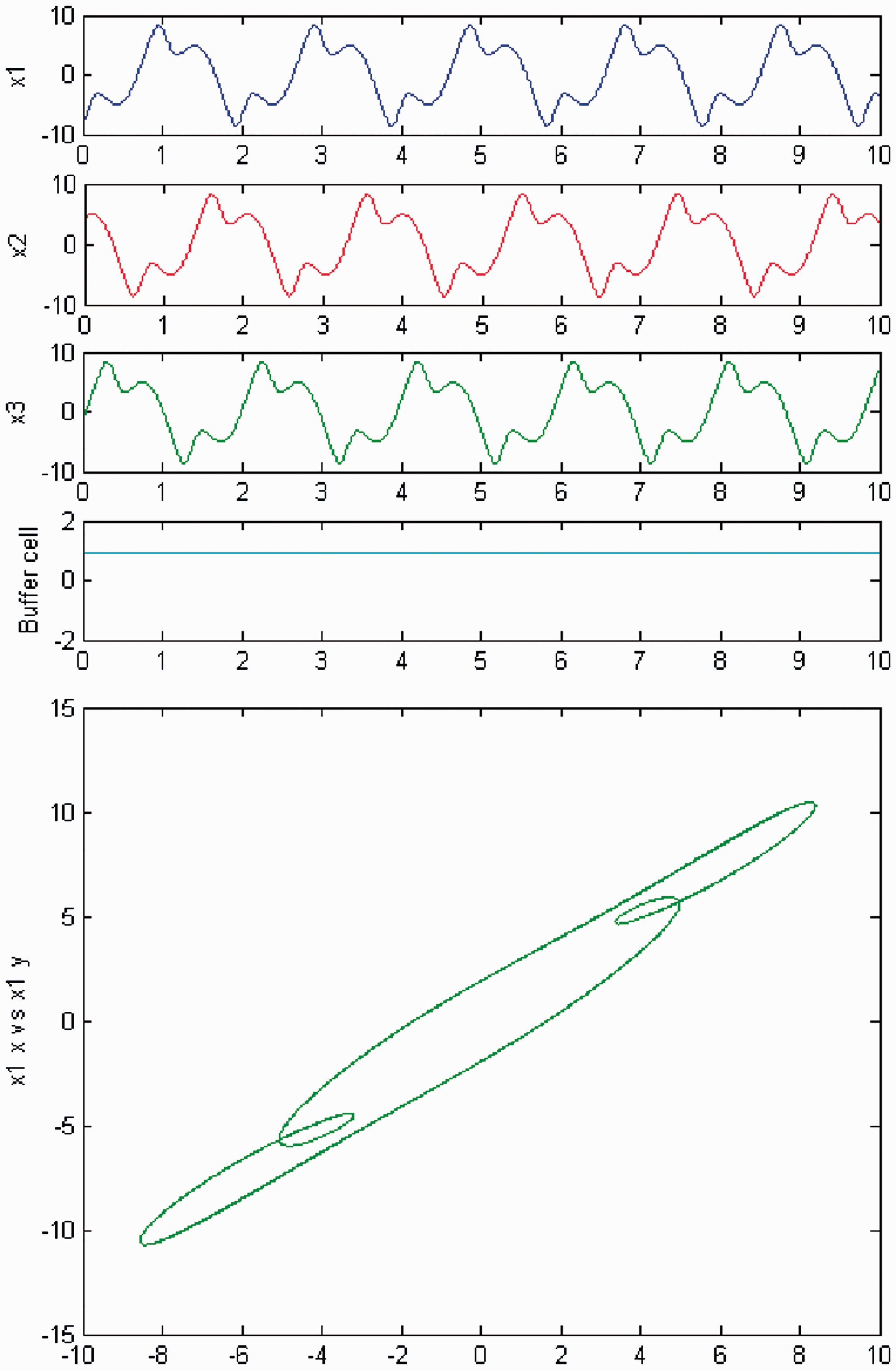
Increasing parameter c further away from the third Hopf point, a change in the qualitative behavior of the system (3) is observed, for the cases of exact and ‘interior’ symmetry. Namely, the cells in the 3-ring appear to show quasiperiodic motion. The ‘buffer’ cell is in equilibrium in the case of exact symmetry (Figure 24) and appears to be quasiperiodic in the case of ‘interior’ symmetry (Figure 25). The full solution is quasiperiodic.

Figure 24.

Simulation of the coupled system (3) for λ = 0 and c₂ ≠ 0. (Top) Time series of the cells in the 3-ring and of the ‘buffer’ cell, for c = 23.6, further away from the third Hopf bifurcation point (HB3). The cells in the 3-ring depict quasiperiodic motion and the ‘buffer’ cell is in a steady state. (Bottom) Phase space of the oscillator x₁.

Figure 25.

Simulation of the coupled system (3) for λ ≠ 0 and c₂ ≠ 0. (Top) Time series of the cells in the 3-ring and of the ‘buffer’ cell, for c = 23.6, further away from the third Hopf bifurcation point (HB3). All cells depict quasiperiodic motion. (Bottom) Phase space of the oscillator x₁.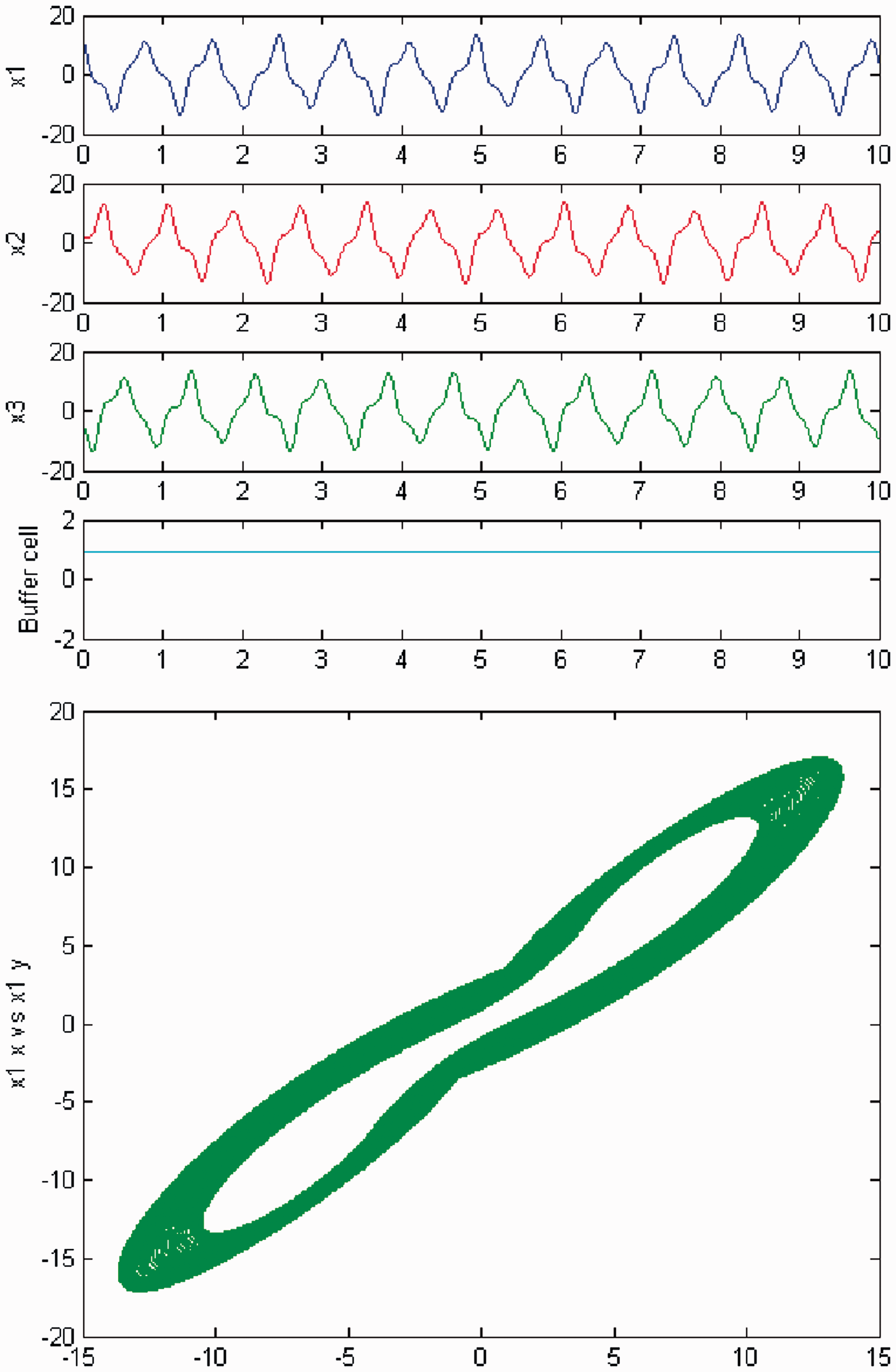

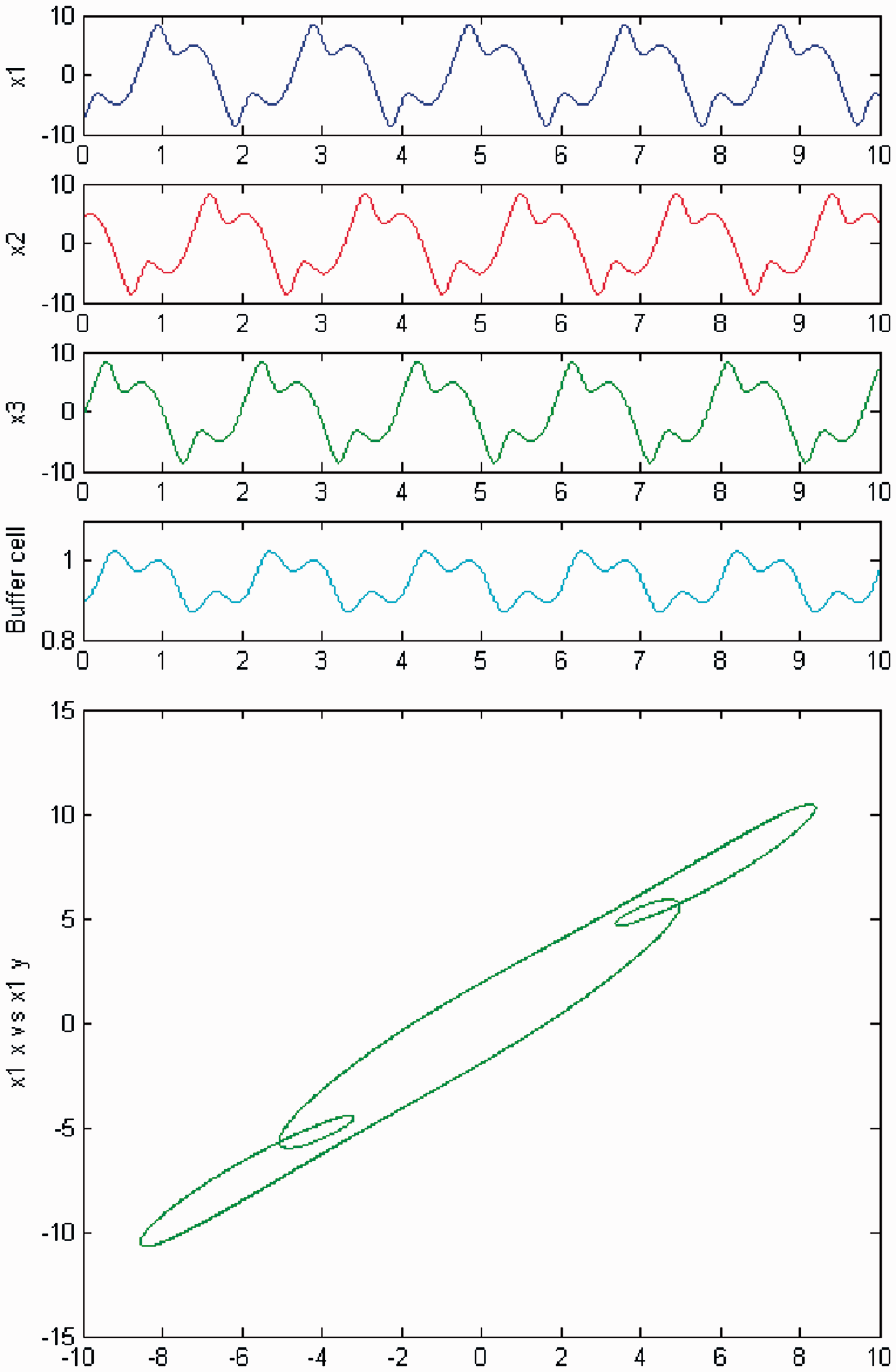
We persist in the increase of parameter c, and a new qualitative change in the behavior of the coupled cell system (3) is observed. Cells in the 3-ring show chaotic motion (see Figures 26 and 27). The ‘buffer’ cell is in a steady state for λ = 0 and in a chaotic state for λ ≠ 0.

Figure 26.

Simulation of the coupled system (3) for λ = 0 and c₂ ≠ 0. (Top) Time series of the cells in the 3-ring and of the ‘buffer’ cell, for c = 29. The cells in the 3-ring exhibit chaotic motion. The ‘buffer’ cell is in a steady state. (Bottom) Phase space of the oscillator x₁.

Figure 27.

Simulation of the coupled system (3) for λ ≠ 0 and c₂ ≠ 0. (Top) Time series of the cells in the 3-ring and of the ‘buffer’ cell, for c = 29. All cells in the network depict chaotic motion. (Bottom) Phase space of the oscillator x₁.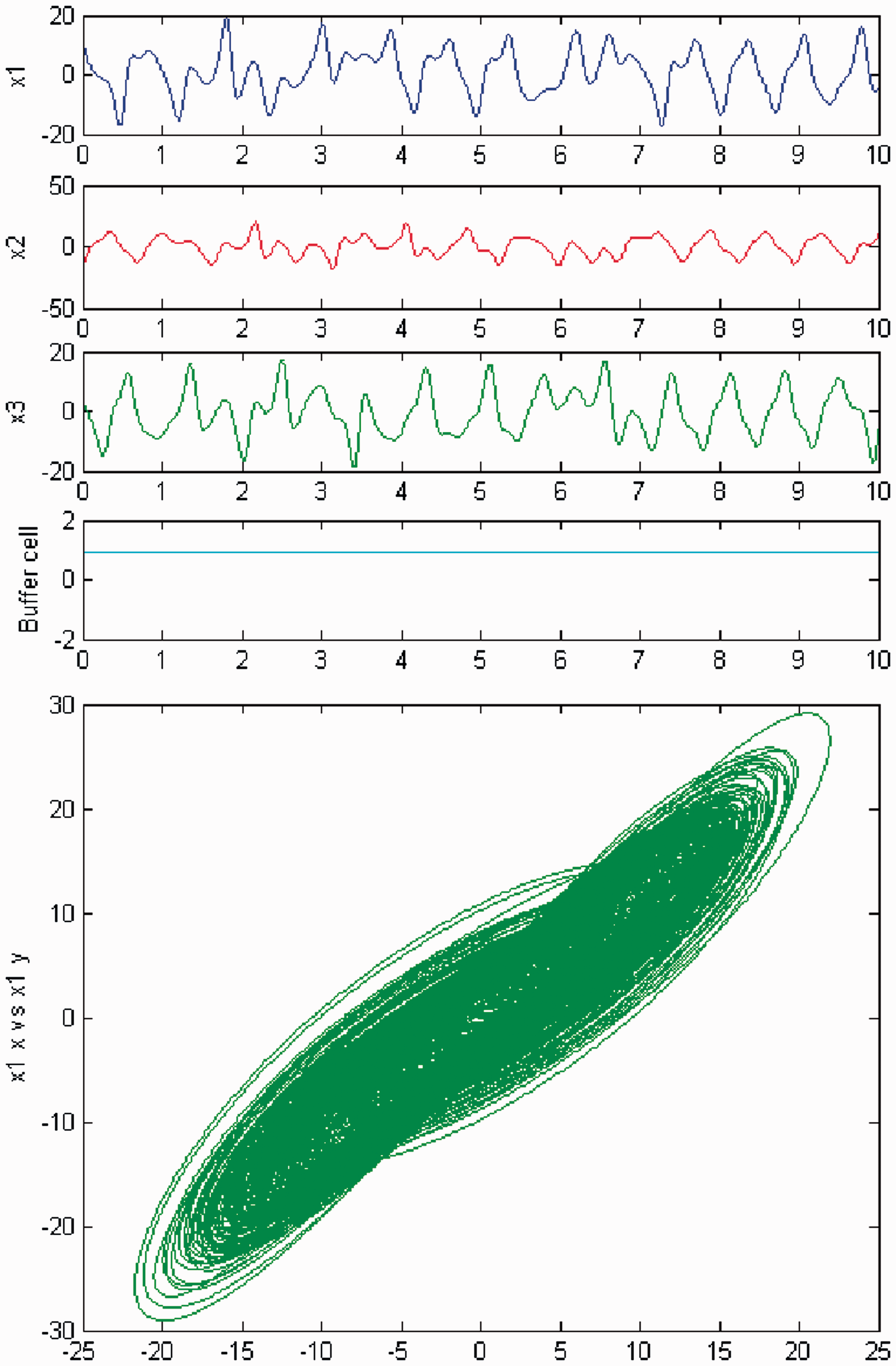

3.3. Discussion

The schematic bifurcation diagram of the coupled system (3) is reproduced in Figure 28. This is a schematic bifurcation diagram of a sequence of three Hopf bifurcations, followed by a cascade of period-doubling bifurcations, and period-halving bifurcations. The first Hopf bifurcating branch emanates from a trivial branch of steady states. Note that, for the parameter region considered here, we do not observe, in the networks in Figure 1(b), the period-halving bifurcations. We have stopped in the chaotic state, after the period-doubling bifurcations.

Figure 28.

Schematic (partial) bifurcation diagram for the coupled cell system (3), near the equilibrium point. Solid lines represent stable solutions. HBi, i = 1,2,3, are Hopf bifurcation points, PD are period-doubling bifurcations, PH are period-halving bifurcations, PO are periodic solutions, and QP are quasiperiodic states.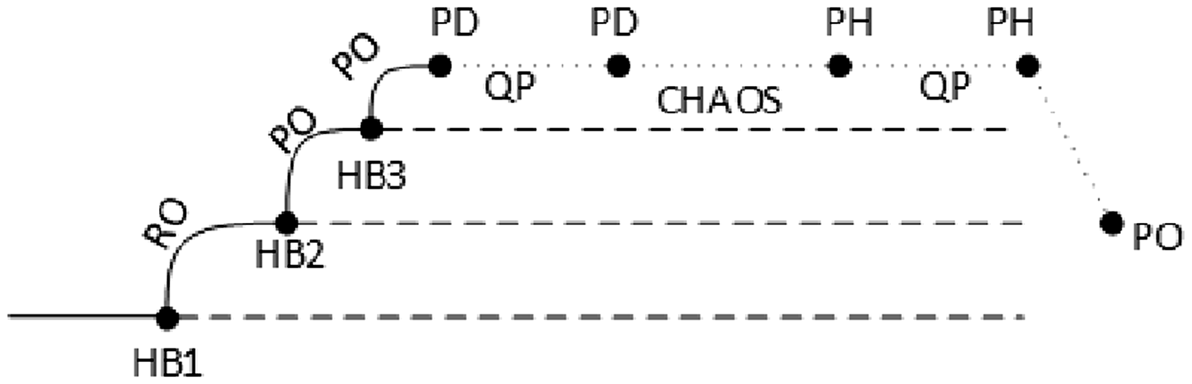

The solutions arising after the primary Hopf bifurcation point are explained by the equivariant Hopf theorem for coupled cell systems in the symmetric case, and the interior symmetry-breaking Hopf theorem for coupled cell systems with ‘interior’ symmetry.

The secondary branch represented in Figure 28 appears through a secondary Hopf bifurcation, along the primary branch at the second Hopf bifurcation point (HB2). The tertiary branch occurs along the secondary branch at the third Hopf bifurcation point (HB3). In this parameter region the solution is periodic, with the same symmetry type as in the primary and secondary branches. Further away along this branch, the coupled cell system (3) evolves to complex dynamical behavior. First, quasiperiodic solutions start to be visible; these solutions are then followed, as the parameter c is increased, by chaotic patterns. This suggests the occurrence of several period-doubling bifurcations in the system.

For the networks in Figure 1(a), proceeding with the increment of the value of c, we note that the system is pulled back from chaos, and quasiperiodic motion reappears. The bifurcations associated with the latter changes in the qualitative behavior of a system are period-halving bifurcations. Incrementing c for the last time, the quasiperiodic solutions disappear, and the coupled cell system (3) again produces a stable Z₃ rotating wave.

Relaxation oscillations are observed for the four networks in Figure 1, after the first Hopf bifurcation point. Relaxation oscillations are solutions characterized by long periods of quasi-static behavior interspersed with short periods of rapid transition, commonly seen in fast–slow systems (Krupa and Szmolyan, 2001). In previous work (Antoneli et al., 2008, 2010; Pinto, 2012), relaxation oscillations were found after the cascade of three Hopf bifurcations points. There, the authors have considered networks of two coupled rings of cells coupled to a ‘buffer’ cell (Antoneli et al., 2008, 2010) or coupled to each other (Pinto, 2012). One of the rings possessed Z₃ or D₃ symmetry, and the other had Z₅ or D₅ symmetry. The authors found relaxation oscillation phenomena further away from the third Hopf bifurcation point. The full solution of the rings was quasiperiodic in that parameter regime. In addition, quasiperiodic solutions and chaos were never seen in the cells of the two coupled rings for the region of parameters considered in the studies Antoneli et al. (2008, 2010) and Pinto (2012). We must note that the internal dynamics of the cells in the rings used there were much simpler than the ones considered in the present research.

Thus, the small networks of one ring of cells coupled to a ‘buffer’ cell in Figure 1 reveal extraordinary dynamical features. Some of these features are certainly explained by the network architecture; nevertheless, the others, such as the route to chaos and returning from chaos, are most certainly attributed to the internal dynamics of the cells, in this case, the Chen oscillator. The Chen oscillator possesses a rich variety of dynamical features for certain parameter regions (Ueta and Chen, 2000; Lu et al., 2002; Li et al., 2004).

4. Conclusions

Four networks of one ring of three cells coupled to a ‘buffer’ cell with exact and ‘interior’ Z₃ and D₃ symmetry groups were considered here. The internal dynamics of each cell were modeled by the Chen oscillator. Peculiar dynamical patterns arise as the parameter c of the Chen oscillator is varied. The symmetry of the networks restricts the behavior of the associated coupled cell systems. Nevertheless, features like quasiperiodicity and chaos seem to appear due to the internal dynamics, the Chen oscillator. Thus, the symmetry is a strong property of the system but its restrictions may be overdue by the properties of the internal dynamics of the cells. Future work will focus on addressing this last issue, namely network architecture versus cells’ internal dynamics: which one defines the dynamics? Moreover, we will address the role of the basin of attraction of the Chen chaotic attractor, in the cases where the networks are ‘pulled back’ from chaos. It was proved that, for a single Chen oscillator, this basin of attraction has the riddled property, based on Milnor’s definition, and any neighborhood of the Chen ‘strange’ attractor contains repelled sets with positive Lebesgue measures (Liu et al., 2007).

Footnotes

Acknowledgement

We thank the anonymous reviewers for their valuable comments and helpful suggestions.

Funding

The authors wish to thank Fundação Gulbenkian, through Prémio Gulbenkian de Apoio à Investigação 2003, and the Polytechnic of Porto, through the PAPRE Programa de Apoio à Publicação em Revistas Científicas de Elevada Qualidade, for financial support. The authors were partially funded by the European Regional Development Fund through the program COMPETE and by the Portuguese Government through the FCT – Fundação para a Ciência e a Tecnologia (project PEst-C/MAT/UI0144/2013). The research of Ana Carvalho was partially supported by the FCT (grant SFRH/BD/96816/2013).

References

Aguiar

Ashwin

Dias

(2011) Dynamics of coupled cell networks: Synchrony, heteroclinic cycles and inflation. Journal of Nonlinear Science 21(2): 271–323.

Antoneli

Dias

Paiva

(2007) Hopf bifurcation in coupled cell networks with interior symmetries. SIAM Journal on Applied Dynamical Systems 7: 220–248.

Antoneli F, Dias A and Pinto C (2008) Rich phenomena in a network of two ring couple through a ‘buffer’ cell. In: Proceedings of the 2nd conference on nonlinear science and complexity NSC.

Antoneli

Dias

Pinto

(2010) Quasi-periodic states in coupled rings of cells. Communications in Nonlinear Science and Numerical Simulation 15(4): 1048–1062.

Boccaletti S, Latora V, Moreno Y, et al. (2006) Complex networks: Structure and dynamics. Physics Reports 424(4–5): 175–308.

Boulkroune

Msaad

(2012) Fuzzy adaptive observer-based projective synchronization for nonlinear systems with input nonlinearity. Journal of Vibration and Control 18(3): 437–450.

Chen

Ueta

(1999) Yet another chaotic attractor. International Journal of Bifurcation and Chaos 9(7): 1465–1466.

Ermentrout B (2006) XPPAUT® – The differential equations tools, version 5.98. Available at: http://www.math.pitt.edu/∼bard/xpp/xpp.html (accessed September 2014).

Golubitsky

Stewart

(2006) Nonlinear dynamics of networks: The groupoid formalism. Bulletin of the American Mathematical Society 43: 305–364.

10.

Golubitsky

Nicol

Stewart

(2004a) Some curious phenomena in coupled cell networks. Journal of Nonlinear Science 14: 119–236.

11.

Golubitsky

Pivato

Stewart

(2004b) Interior symmetry and local bifurcation in coupled cell networks. Dynamical Systems 19(4): 389–407.

12.

Golubitsky

Stewart

Schaeffer

(1988) Singularities and Groups in Bifurcation Theory (Applied Mathematical Sciences 69, vol. II), New York, NY: Springer-Verlag.

13.

Golubitsky

Stewart

Torok

(2005) Patterns of synchrony in coupled cell networks with multiple arrows. SIAM Journal of Applied Dynamical Systems 4(1): 78–100.

14.

Gong

Liu

Wang

(2014) Chaotic system synchronization with tridiagonal structure and its initial investigation in complex power systems. Journal of Vibration and Control 3(20): 447–457.

15.

Krupa

Szmolyan

(2001) Relaxation oscillation and canard explosion. Journal of Differential Equations 174(2): 312–368.

16.

Lin

Liao

Yan

(2005) Synchronization of unidirectional coupled chaotic systems with unknown channel time-delay: Adaptive robust observer-based approach. Chaos, Solitons and Fractals 26: 971–978.

17.

Chen

Tang

(2004) On stability and bifurcation of Chen’s system. Chaos, Solitons and Fractals 19(5): 1269–1282.

18.

Liu

Chen

(2007) The basin of attraction of the Chen attractor. Chaos, Solitons and Fractals 34(5): 1696–1703.

19.

Zhou

Chen

(2002) Local bifurcation of the Chen system. International Journal of Bifurcation and Chaos 12: 2257–2270.

20.

Mahmoud

Ahmed

(2011) Modified projective synchronization and control of complex Chen and Lü systems. Journal of Vibration and Control 8(17): 1184–1194.

21.

Mahmoud

Arafa

(2013) Passive control of n-dimensional chaotic complex nonlinear systems. Journal of Vibration and Control 7(19): 1061–1071.

22.

Matias

Gollo

Carelli

(2011) Anticipated synchronization in a biologically plausible model of neuronal motifs. Physical Review E 84: 021922.

23.

Michiels

(2010) Stability analysis of oscillatory systems subject to large delays: A synchronization point of view. Journal of Vibration and Control 7–8(16): 1087–1110.

24.

Pikovsky

Rosenblum

Kurths

(2001) Synchronization, A Universal Concept in Nonlinear Sciences, Cambridge: Cambridge University Press.

25.

Pinto

(2012) Exotic dynamics in networks of coupled rings of cells. International Journal of Bifurcation and Chaos 22(3): 1250064 13 pp.

26.

Pinto

Golubitsky

(2006) Central pattern generators for bipedal locomotion. Journal of Mathematical Biology 53: 474–489.

27.

Stewart

Golubitsky

Pivato

(2003) Symmetry groupoids and patterns of synchrony in coupled cell networks. SIAM Journal of Applied Dynamical Systems 4(2): 609–646.

28.

Ueta

Chen

(2000) Bifurcation analysis of Chen’s attractor. International Journal of Bifurcation and Chaos 10: 1917–1931.

29.

Zhu

(2013) Flocking of multi-agent non-holonomic systems with proximity graphs. IEEE Transactions on Circuits and Systems 60(1): 199–210.