State space analysis of forest fires

Abstract

This paper studies forest fires from the perspective of dynamical systems. Burnt area, precipitation and atmospheric temperatures are interpreted as state variables of a complex system and the correlations between them are investigated by means of different mathematical tools. First, we use mutual information to reveal potential relationships in the data. Second, we adopt the state space portrait to characterize the system’s behavior. Third, we compare the annual state space curves and we apply clustering and visualization tools to unveil long-range patterns. We use forest fire data for Portugal, covering the years 1980–2003. The territory is divided into two regions (North and South), characterized by different climates and vegetation. The adopted methodology represents a new viewpoint in the context of forest fires, shedding light on a complex phenomenon that needs to be better understood in order to mitigate its devastating consequences, at both economical and environmental levels.

Keywords

Dynamical systems state space mutual information multidimensional scaling hierarchical clustering forest fires

1. Introduction

Forest fires (FFs) have a great impact on the environment and the economy (Logan et al., 2003; Rittmaster et al., 2006). Burnt areas correspond directly to flora and fauna losses, ecosystem damage and soil degradation (Smith et al., 2000; Certini, 2005). Long-term consequences are the modification of the water cycle, replacement of autochthonous vegetation by invasive species (Brooks et al., 2004), increase in carbon dioxide emissions (Page et al., 2002) and climate change (Flannigan et al., 2000) (e.g. global warming and extreme weather events). In fact, wildfires can be regarded as positive feedback loops acting on the climate complex system (CS), simultaneously potentiating and being potentiated by climate changes (Dale et al., 2001; Kirilenko and Sedjo, 2007).

FF propagation depends on many factors, such as weather conditions, terrain orography and type of vegetation. Moreover, the effectiveness of detection and suppression measures is fundamental in order to mitigate fire impact (Chandler et al., 1983). Fire size patterns and spatiotemporal distributions provide valuable information for deciding about preventive measures, helping in identifying possible hazards, and in planning strategies for prevention, detection and suppression (Tenreiro Machado and Lopes, 2014).

Standard statistical methods have proved to be inadequate for analyzing extreme fire events (Holmes et al., 2008) as they are not capable of capturing all characteristics underneath fire dynamics (Alvarado et al., 1998). FFs exhibit complex spatiotemporal correlations, characterized by long-range memory and absence of a characteristic length-scale (Malamud et al., 1998; Ricotta et al., 1999; Reed and McKelvey, 2002; Telesca et al., 2005; Song et al., 2006). Those features are explained by the self-organized critical (SOC) (Bak, 1990) and highly optimized tolerance (HOT) models, proposed to explain fire behavior (Grassberger and Kantz, 1991; Drossel and Schwabl, 1992; Carlson and Doyle, 1999; Moritz et al., 2005).

Ricotta et al. (1999) analyzed FF data for the region of Liguria (Italy), covering the years 1986–1993. They concluded that there is a power-law (PL) relationship between the frequency of occurrence of the event and the burnt area (size). Malamud et al. (1998) analyzed FFs in the USA and Australia and showed that FFs exhibit a PL dependence frequency versus size, over many orders of magnitude. A simple fire model was proposed and it was concluded that actual FFs can be directly associated with the model. Deviations from PL behavior, observed in certain cases, were explained by Song et al. (2006). They examined the SOC and fractal characteristics of FFs in China and hinted at actual FF protection. Reed and McKelvey (2002) proposed empirical frequency–size distributions, derived from real data in six regions in North America, concluding that a simple PL distribution of sizes may be too simple to describe the distributions over their full range. They developed a stochastic model for the spread and extinguishment of FFs to examine the necessary conditions for PL behavior. FF time-scaling was addressed by Telesca et al. (2005), who characterized the temporal distribution of fires occurring in Gargano (Italy), known for its high density of fires. They concluded that the point process of fire events is a fractal process with a high degree of time-clusterization. Time-scales are of the order of a few days and the fire process tends to be less time-clustered with an increase in the burnt area. The time-scaling properties of yearly FF sequences occurring in the Reggio Calabria (Italy) region were studied by Lasaponara et al. (2005). Their results show that FFs exhibit a strong degree of time-clusterization.

The HOT conceptual framework, as an alternate to SOC, was used to explain the formation of scale-invariant patterns in CSs (Carlson and Doyle, 1999). It emphasizes that PL behavior results from optimization of tradeoffs between system yield and tolerance to risk, which drives the system to a specific spatial configuration. Moritz et al. (2005) studied historical fire catalogs and proposed a detailed fire simulation model. They concluded that both are in agreement with the HOT concept. Boer et al. (2008) showed that FF size distributions are closely related to distributions of weather events. Zheng et al. (2008) investigated the PL scaling behavior of FFs and weather parameters by means of a detrended fluctuation analysis method. They verified that temperature, relative humidity and precipitation data reveal characteristics similar to FFs. Their reported findings were shown to be useful for quantifying the underlying dynamics of FF and weather parameters, and for understanding the relationship between them.

In this paper we study FFs from the perspective of dynamical systems. Burnt area and weather variables, such as precipitation and atmospheric temperatures, are interpreted as state variables of a CS and the correlations between them are investigated on an annual basis using different mathematical tools. First, we propose the mutual information concept to unveil potential relationships in the data. Second, we adopt the state space portrait to characterize the system behavior. Third, we compare the state space curves and use clustering and visualization tools, namely hierarchical clustering and multidimensional scaling. Several long-range patterns emerge in FF time-lines. Our study focuses on data for Portugal (excluding Azores and Madeira), covering the time period from 1980–2003. We divide the Portuguese territory into two regions (North and South), as they present different climates and vegetation. The adopted methodology and tools represent a new viewpoint in the context of FF analysis, shedding light on a complex phenomenon that needs to be better understood in order to mitigate its severe consequences. The paper reveals the difficulties in forecasting future events based on a limited set of variables. However, it is clear that the emergence of clusters corresponds to complex dynamical effects. In fact, the emerging patterns resemble those of chaotic systems, leading to poor predictability. On the other hand, the study demonstrates that the results point towards measuring a richer set of environmental variables and the recording of longer time-series in order to establish a solid basis for computer data analysis systems.

Bearing these ideas in mind, this paper is organized as follows. Section 2 introduces some fundamental mathematical concepts. Section 3 describes the experimental dataset and characterizes the data using simple statistics. Section 4 analyzes the data by means of state space portrait and compares the state space curves using clustering and visualization tools. Finally, Section 5 presents the main conclusions.

2. Mathematical background

This section presents the mathematical tools used to process the data, namely mutual information (MI), state space portrait (SSP), hierarchical clustering (HC) and multidimensional scaling (MDS).

2.1. Mutual information

The MI statistical concept originated from the area of information theory. MI measures the statistical dependence between two random variables and can be interpreted as the amount of information that one variable ‘contains’ about the other (Shannon, 2001). Recently, MI has been used as an approach to analyze different CSs (Fraser and Swinney, 1986; Matsuda, 2000; Tenreiro Machado and Lopes, 2013). Mathematically, for two discrete random variables (X,Y), the MI, I(X,Y) is given by

I (X, Y) = \sum_{y \in Y} \sum_{x \in X} p (x, y) \cdot \log (\frac{p (x, y)}{p (x) \cdot p (y)})

(1)

where, p(x) and p(y) represent the marginal probability distribution functions of X and Y, respectively, and p(x,y), is the joint probability distribution function. MI is always symmetric and nonnegative, that is, I(X,Y) = I(Y, X) ≥ 0.

2.2. State space portrait

A n-dimensional dynamical system can be represented by a set of first-order differential equations governing n state variables, $x_{1} (t), x_{2} (t), \dots, x_{n} (t)$ , where t represents time. Such equations are obtained from the system input–output functional relationship (i.e. the system model), for a given set of state variables. Knowing the state variables at time t = t₀ and the system inputs for t ≥ t₀, we can determine the system behavior for t ≥ t₀. The state space consists of the set of all possible states, each one corresponding to a unique point. As t evolves, we get sequences of points describing trajectories in the state space. The set of trajectories is the SSP. For first-, second- and third-order systems, the SSP can be depicted on a map and the system behavior can be inferred from the corresponding graphical representation (Polderman and Willems, 1998).

2.3. Hierarchical clustering

Clustering analysis organizes data into groups (clusters) such that there is a high/low intra/inter-cluster similarity between objects. Clustering exposes the internal structures of the data, underlying rules and patterns. It has been adopted in data mining, machine learning, pattern recognition, image analysis and bioinformatics, among others (Hartigan, 1975).

There are two types of clustering: partitional and hierarchical. In partitional clustering, different partitions are created and then evaluated by means of some criterion (e.g. k-means (Jain, 2010)). In HC a hierarchy of object clusters is built. This is typically done by means of heuristic algorithms. In agglomerative clustering the algorithm starts with each object in its own cluster and, at each step, it finds the best (most similar) pair of clusters to merge into a new cluster. It iterates until all clusters are merged together. In divisive clustering the algorithm starts with all items in a single cluster, at each step, it chooses the best way to split the cluster into two and, recursively, operates on both new-formed clusters. The iterations stop when each object is in its own cluster.

Both in agglomerative and divisive clustering, the clusters are generated by evaluating the inter-cluster dissimilarity. A metric (i.e. a measure of the distance between pairs of objects) and a linkage criterion (i.e. the definition of the dissimilarity between clusters as a function of the pairwise distances between objects) are adopted to quantify the inter-cluster dissimilarity. Mathematically, for two clusters, U and V, a metric is used to measure the distance between objects, $d (x_{U}, x_{V}), x_{U} \in V$ and $x_{V} \in V$ . Based on that metric, the maximum, minimum, or average, linkage criterion is adopted, that is, respectively

d_{max} (U, V) = {max}_{x_{U} \in U, x_{V} \in V} d (x_{U}, x_{V})

(2)

d_{min} (U, V) = {min}_{x_{U} \in U, x_{V} \in V} d (x_{U}, x_{V})

(3)

d_{ave} (U, V) = \frac{1}{∥ U ∥ ∥ V ∥} \sum_{x_{U} \in U, x_{V} \in V} d (x_{U}, x_{V})

(4)

The results of HC are usually presented in a dendrogram, where the similarity between two objects is represented by the height of their lowest common internal node.

2.4. Multidimensional scaling

MDS is a set of techniques for visualizing similarities/dissimilarities between objects in a dataset (Cox and Cox, 2000). MDS generates maps describing the objects’ locus in the perspective that, if they are perceived to be similar/dissimilar to each other, then they are placed on the map close/distant to/from each other. MDS provides an intuitive and useful visual representation of complex relationships present among objects. In metric MDS the input is an n × n symmetric matrix, M, of object pairwise similarities/dissimilarities, where n denotes the number of objects in the dataset. The measure for quantifying similarities/dissimilarities depends of the researcher’s choice and can be selected based on multiple criteria. MDS assigns a point to each object, rearranging the object’s coordinates in a m-dimensional space. Using an optimization algorithm, it evaluates different configurations and outputs a coordinate matrix representing the configuration that best reproduces the observed similarities/dissimilarities. For m = 2 and m = 3 the results are easily represented in a graph, where the orientation of the axes is arbitrary. The distances between points are always the same, independently of any rotation or translation of the MDS map, and can be chosen in order to get a clearer visualization. Stress and Shepard plots are usually adopted for accessing MDS results. The stress is a function of the number of dimensions m. The corresponding diagram is a monotonic decreasing chart, which is useful to decide the ‘best’ dimension m, as a compromise between stress reduction and number of dimensions. The Shepard plot, maps the reproduced versus the observed similarities/dissimilarities. A narrow scatter around a 45° line indicates a good fit.

3. Brief description of the dataset

This section describes the dataset used in this study (i.e. FFs, precipitation and temperature) and complements the presentation with simple statistics.

We consider the Portuguese continental territory divided into the North (N) and South (S) regions as shown in Figure 1. These regions correspond to different climate, vegetation and orography conditions, which influence fire behavior. The time period of analysis is limited to years 1980–2003, which is imposed by the data available.

Figure 1.

Location of the two Portuguese regions studied.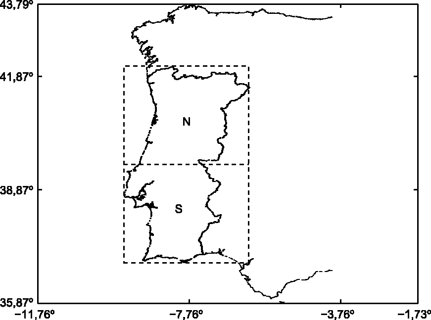

A catalog of FFs is compiled by the Portuguese Instituto da Conservação da Natureza e das Florestas (INCF), and is available online at http://www.icnf.pt/portal/florestas/dfci/inc/estatisticas. Each data record contains information about the date of the event, time (with one-minute resolution), geographic location (expressed in latitude and longitude coordinates) and size (quantified by the burnt area, expressed in hectares). All occurrences are included, independently of their cause, namely natural factors, human negligence and human intent.

The data is pre-processed by calculating the daily burnt area in each region. Figure 2 shows the burnt area for regions N and S. We adopt a circular time-scale to represent the time evolution of fire within the period 1980–2003. The circular time evolves along an Archimedean spiral with its origin at the center of the circumferences defined by

θ = 2 π [\frac{t}{T} + (i - 1980)], r = p + q θ

(5)

where (r,θ) denotes the radius and angle coordinates, respectively,

p = q = 1, i = 1980, \dots, 2003

and t and T represent time and one year. The daily burnt area, B, expressed in logarithmic units, is related to the color of the marks. As can be seen, most events are depicted on the graph in the area corresponding to summer. Moreover, region N is more prone to fire than region S, which is justified by the availability of denser areas of forest and vegetation.

Figure 2.

Time evolution of the daily burnt area, during the period 1980–2003: (a) region N; (b) region S.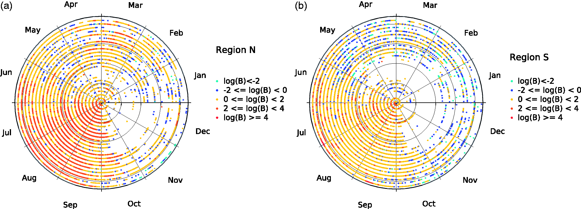

Data on precipitation was collected at the Instituto Português do Mar e da Atmosfera (IPMA) https://www.ipma.pt/en/. The database contains information of daily precipitation for Portugal, in a regular grid with 0.2° × 0.2° resolution, for the period 1950–2003. The gridded data was obtained based on records from 806 meteorological stations, interpolating the original data using the Kriging method (Belo-Pereira et al., 2011).

We pre-processed the gridded database, calculating the total daily precipitation for regions N and S in the period 1980–2003.

The source of temperature data was the National Aeronautics and Space Administration (NASA) website (http://data.giss.nasa.gov/gistemp/station_data/). Each data series consists of the average temperatures per month, expressed in Celsius degrees, of several worldwide meteorological stations. We use temperature time-series of Porto and Lisbon to represent the N and S regions of Portugal, respectively. This option is justifiable by the existence of accurate data for both cities and because Portugal is a small country, making the inclusion of other centers unnecessary. Thus, using data from one place to characterize each region is a good approximation. We pre-processed the data, filling occasional gaps of one month (represented on the original dataset by the value 999.9) by temperature values calculated using linear interpolation between the two adjacent points. The distinct number of days of each month and the leap years were taken into account. The data was then interpolated linearly in order to get daily mean temperatures (Tenreiro Machado and Lopes, 2012; Lopes and Tenreiro Machado, 2014).

In Figure 3 we represent the evolution of the annual total burnt area, mean temperature and precipitation, for regions N and S, over the time period 1980–2003. It can be seen that there is a correlation between burnt area and both mean temperature and precipitation.

Figure 3.

Evolution of the annual burnt area, mean temperature and precipitation, over the time period 1980–2003: (a) region N; (b) region S.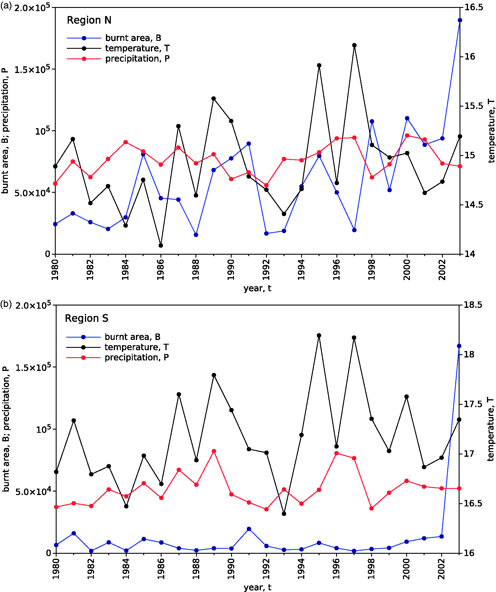

We verify that the previous simple statistics do not capture all the hidden relationships in the data. Therefore, in the next section, several complementary mathematical tools are adopted.

4. Data analysis and results

In this section, data comprising burnt area, precipitation and atmospheric temperatures are interpreted as state variables of a CS and correlations between the variables are investigated on an annual basis. In subsection 4.1, we use MI to analyze the relationships in the data. In Section 4.2, we adopt the SSP to characterize the system’s behavior. Finally, in Section 4.3 we compare the state space curves by means of HC and MDS.

4.1. Mutual information analysis

To calculate the MI, we first generate the annual time-series of daily values

x_{i}^{W} (t) = \sum_{k = 1}^{T} W_{i, k} δ (t - t_{i, k})

(6)

leading to 24 time-series for each variable, where,

W = {B, P, T}

denotes burnt area (B), precipitation (P) and mean temperature (T), respectively. The variable

W_{i, k}

represents daily values,

t_{i, k}

are time-instants (i.e. days), T is the total number of days in one year, and

δ (\cdot)

corresponds to the Dirac delta function.

The annual MI between burnt area and precipitation, I(B,P) and between burnt area and mean atmospheric temperature I(B,T) were calculated, estimating the probabilities by means of the histograms of relative frequencies. For constructing the histograms, we adopt N = 200 bins.

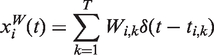
Figures 4 and 5 represent the evolution of the annual MI between burnt area and precipitation, I(B,P), and between burnt area and mean atmospheric temperature I(B,T), for regions N and S, respectively. We can see that, for the two regions, I(B,P) is lower than I(B,T). For region N, I(B,P) is somewhat ‘noisy’, but it stays almost constant over the period 1980–2003, with exception of the years {1990, 2003} and {1997}, where minimum and maximum values of MI are registered, respectively. With respect to I(B,T), in the early years it is almost constant. In year {1988} it reaches a maximum value and, for more recent years, its trend is for decreasing. For region S, I(B,P) is also ‘noisy’, but its trend reflects some increasing over time, except for years {1980, 2003}. The evolution of I(B,T) shows a trend to increase during the first half and to decrease for the second half of the period of analysis.

Figure 4.

Evolution of the annual MI between burnt area and precipitation, I(B,P), and between burnt area and mean atmospheric temperature I(B,T), for region N, during the time period 1980–2003.

Figure 5.

Evolution of the annual MI between burnt area and precipitation, I(B,P), and between burnt area and mean atmospheric temperature I(B,T), for region S, during the time period 1980–2003.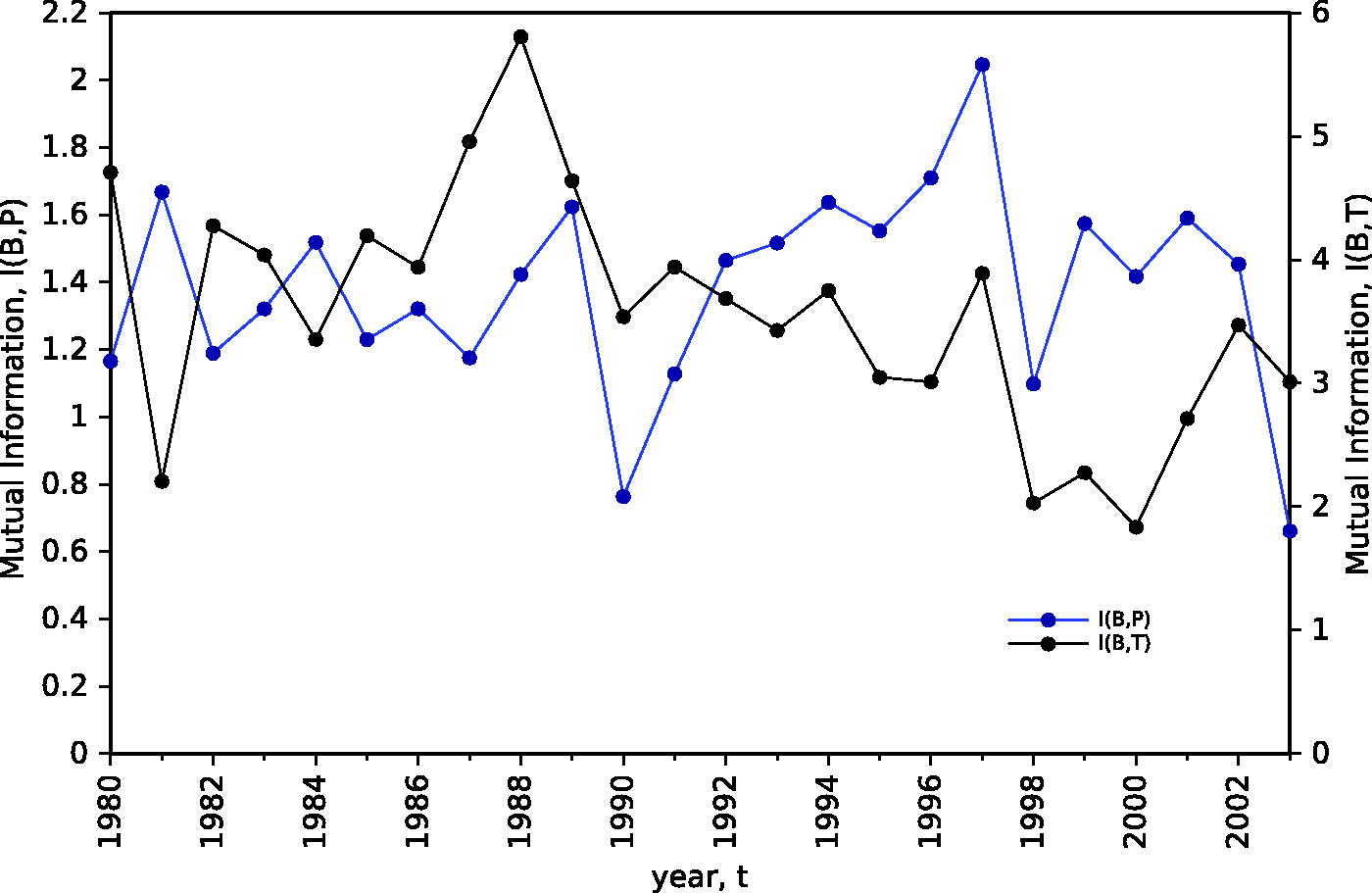

4.2. State space analysis

To generate the SSP we first compute the annual time-series of accumulated burnt area, ${\tilde{X}}_{i}^{B} (t)$ , and accumulated precipitation, ${\tilde{X}}_{i}^{P} (t)$ , which are given by

{\tilde{X}}_{i}^{Z} (t) = \int_{0}^{t} x_{i}^{Z} (u) 1 mu d u, Z = {B, P}

(7)

where, 0 ≤ t ≤ T and t = 0 corresponds to the first day of each year

i = 1980, \dots, 2003

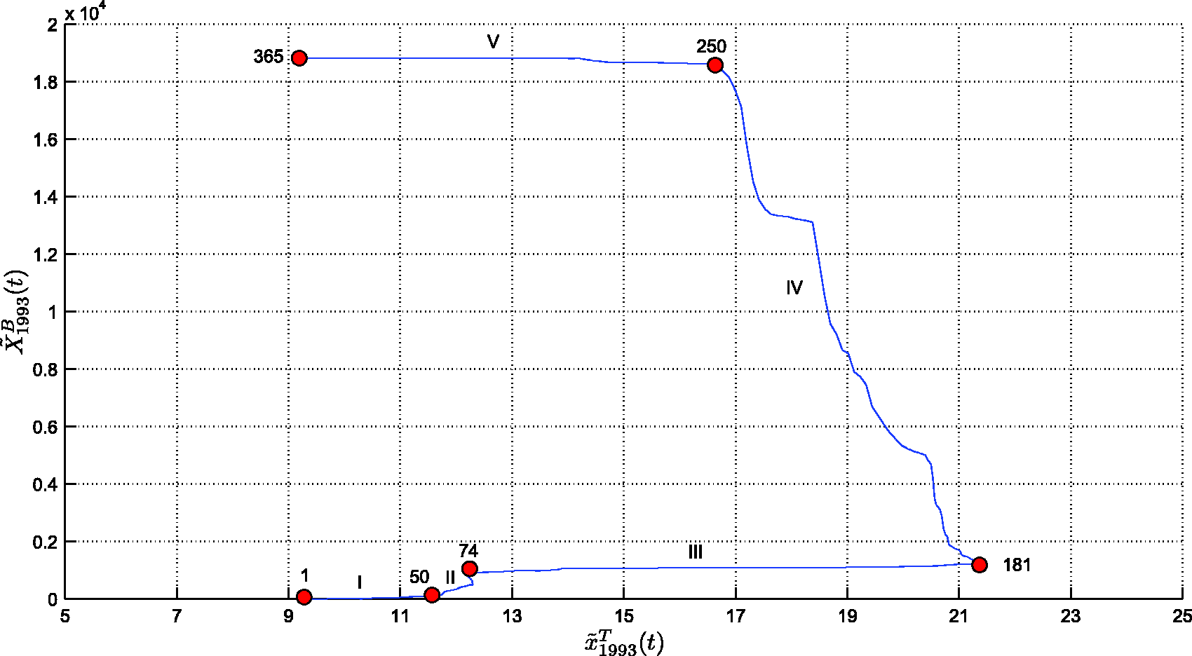
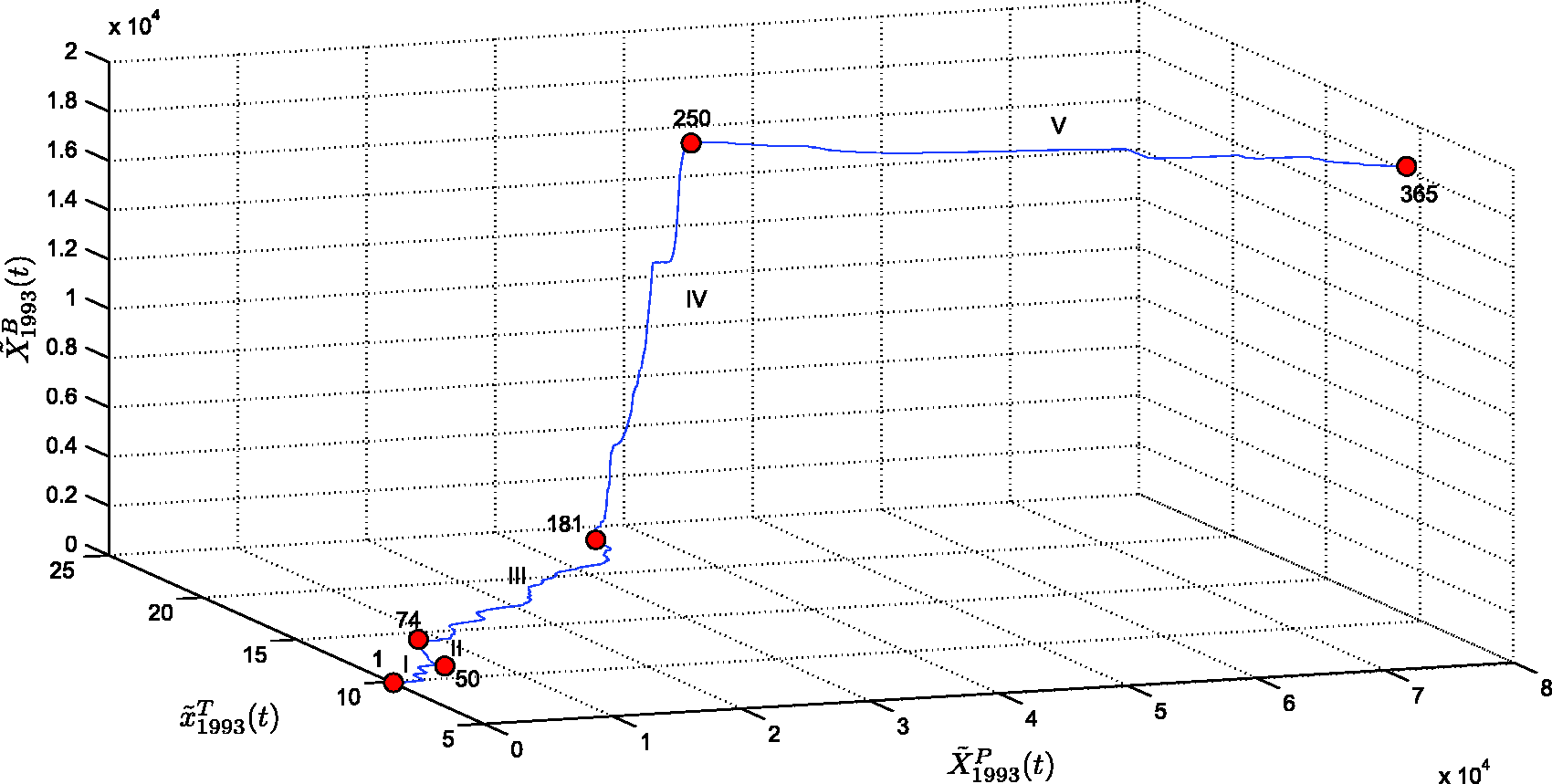
Second, we analyze the annual SSP generated by the three ‘state’ variables: accumulated burnt area, ${\tilde{X}}_{i}^{B} (t)$ , accumulated precipitation, ${\tilde{X}}_{i}^{P} (t)$ and mean atmospheric temperature, $x_{i}^{T} (t)$ , leading to 24 three-dimensional curves.

In this second analysis, to illustrate the methodology, we present the results for year 1993, in region N. Figure 6 depicts the time evolution of the variables, where we can see that the accumulated burnt area, ${\tilde{X}}_{i}^{B} (t)$ , reveals five distinct regimes. Period I corresponds to 1 ≤ t ≤ 50 days (i.e. from January up to mid-February), with negligible fire activity, low temperatures (below 11.7℃) and intermittent periods with precipitation. Period II corresponds to 50 ≤ t ≤ 74 days (i.e. from mid-February up to mid-March). Fire activity increases moderately, temperatures are in the interval [11.7℃,12.3℃] and precipitation is almost absent. In period III, 74 ≤ t ≤ 181 days, (i.e. from mid-March up to end of June), fire activity is low, and temperatures increase up to the interval [12.3℃, 21.3℃] while precipitation is quite intense. Period IV, 181 ≤ t ≤ 250 days, corresponds to the end of June up to the end of August. Fire activity goes up by a large increment. Temperatures stay above 16.5℃ and precipitation is negligible. Finally, in period V, 250 ≤ t ≤ 365 days (from the end of August up to the end of the year), fire activity is again negligible, temperatures decrease continuously and precipitation remains present.

Figure 6.

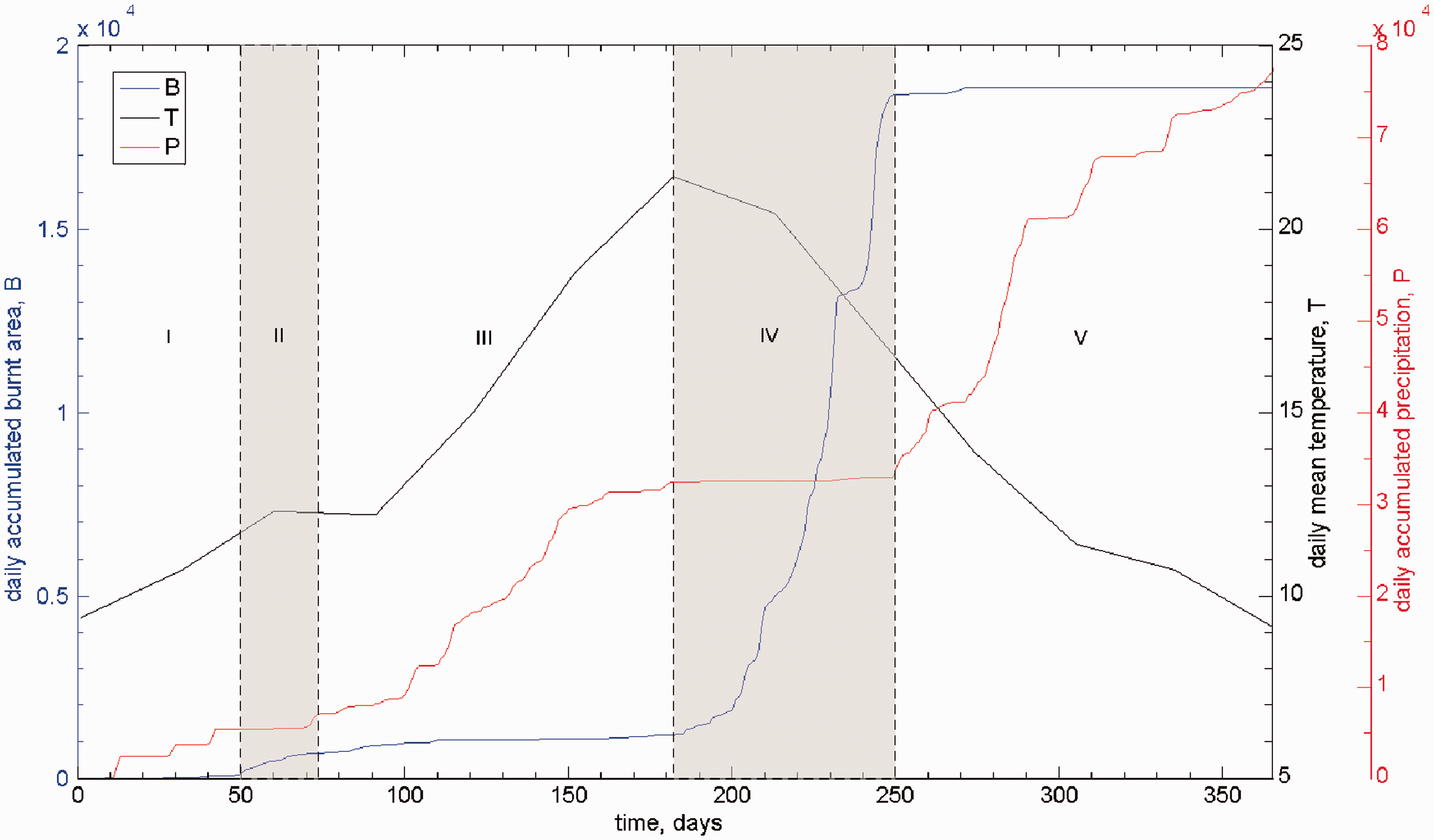
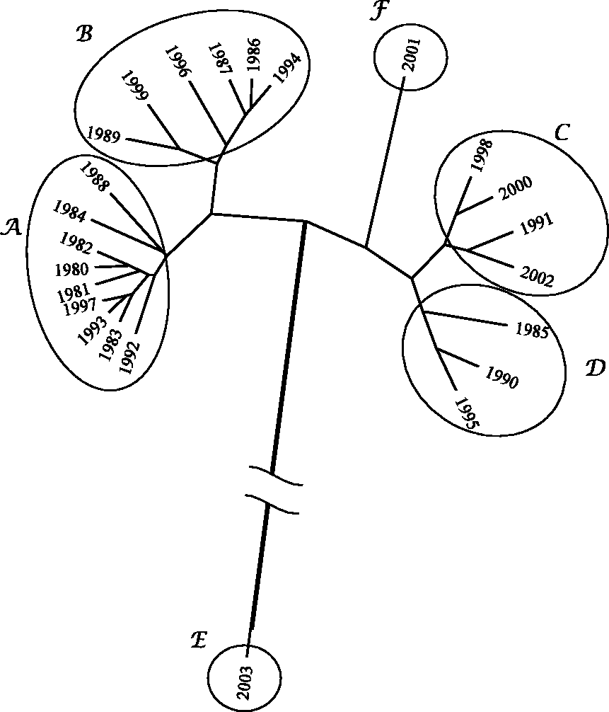
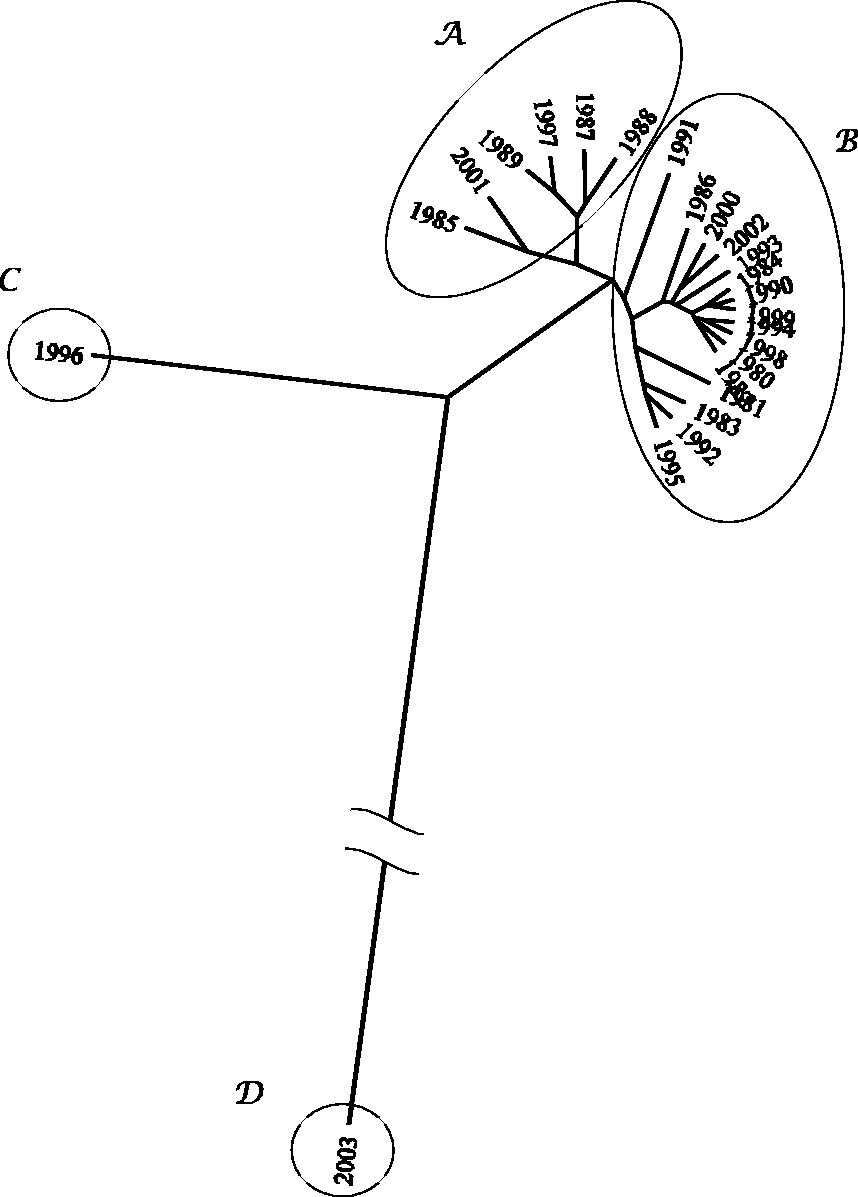
Time evolution of the variables ${\tilde{X}}_{i}^{B} (t), {\tilde{X}}_{i}^{P} (t)$ and $x_{i}^{T} (t)$ , for year i = 1993 and region N.

The relationships between ${\tilde{X}}_{i}^{B} (t)$ , ${\tilde{X}}_{i}^{P} (t)$ and $x_{i}^{T} (t)$ (i = 1993) are presented in Figures 7, 8 and 9, corresponding to the SSP ${\tilde{X}}_{i}^{B} (t)$ vs. ${\tilde{X}}_{i}^{P} (t)$ , ${\tilde{X}}_{i}^{B} (t)$ vs. $x_{i}^{T} (t)$ and ${\tilde{X}}_{i}^{B} (t)$ vs. ${\tilde{X}}_{i}^{P} (t)$ vs. $x_{i}^{T} (t)$ , respectively.

Figure 7.

The SSP ${\tilde{X}}_{i}^{B} (t)$ vs. ${\tilde{X}}_{i}^{P} (t)$ , for year i = 1993 and region N.

Figure 8.

The SSP ${\tilde{X}}_{i}^{B} (t)$ vs. $x_{i}^{T} (t)$ , for year i = 1993 and region N.

Figure 9.

The SSP ${\tilde{X}}_{i}^{B} (t)$ vs. ${\tilde{X}}_{i}^{P} (t)$ vs. $x_{i}^{T} (t)$ , for year i = 1993 and region N.

Figure 10.

Visualization tree generated by the HC algorithm, representing similarities between SSP annual curves, for region N.

Figure 11.

Visualization tree generated by the HC algorithm, representing similarities between SSP annual curves, for region S.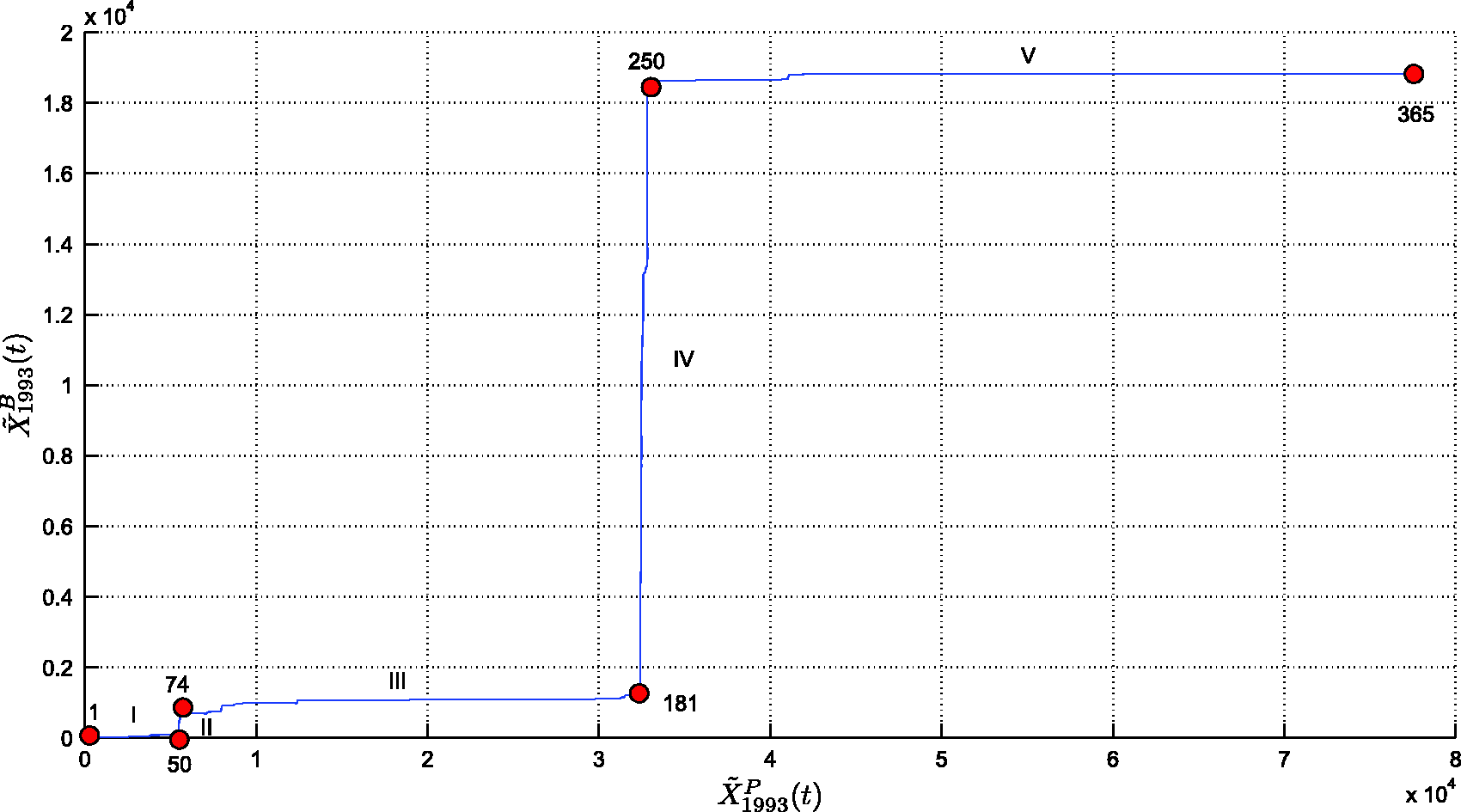

4.3. Clustering analysis and visualization

In this subsection clustering and visualization algorithm are adopted to compare the annual SSP curves and to unveil relationships in the data.

To compare all SSPs we calculate a 24 × 24 dissimilarity matrix $M = [e_{ij}]$ , based on the Euclidean distance $e_{ij} (i, j = 1980, \dots, 2003)$ , between the SSP curves

e_{ij} = \sqrt{(x_{i} - x_{j}) 2 + (y_{i} - y_{j}) 2 + (z_{i} - z_{j}) 2}

(8)

where, (x_i,y_i,z_i) and (x_j,y_j,z_j) represent the coordinates of the SSP curve pairs (i,j), respectively.

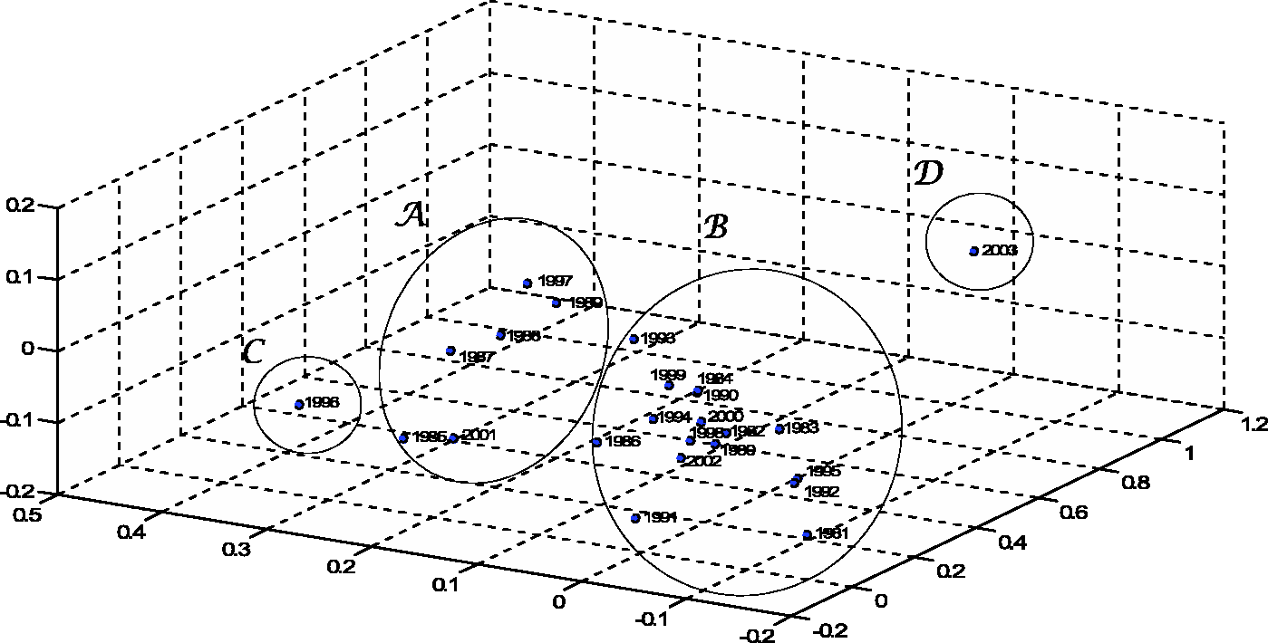
Two visualization trees are generated using HC, corresponding to regions N and S (Figures 10 and 11, respectively). The successive (agglomerative) clustering and average-linkage methods are adopted. The software PHYLIP is used for generating the graphs (http://evolution.genetics.washington.edu/phylip.html). For region N, we can note the emergence of six clusters: $A$ = {1980, 1981, 1982, 1983, 1984, 1988, 1992, 1993, 1997}, $B$ = {1986, 1987, 1989, 1994, 1996, 1999}, C = {1991, 1998, 2000, 2002}, $D$ = {1985, 1990, 1995}, $E$ = {2003} and $F$ = {2001}. For region S, we identify four clusters: $A$ ={1985, 1987, 1988, 1989, 1997, 2001}, $B$ = {1980, 1981, 1982, 1983, 1984, 1986, 1990, 1991, 1992, 1993, 1994, 1995, 1998, 1999, 2000, 2002}, C = {1996} and $D$ = {2003}.

As an alternative to HC and visualization trees we adopt MDS, feeding the algorithm with matrix M. The MDS maps for m = 3 are depicted in Figures 12 and 13, corresponding to regions N and S, respectively. As said previously, a shorter (larger) distance between two points on a map means that the corresponding objects are more similar (distinct). The clusters identified previously are also depicted. We can say that both visualization trees and MDS maps allow good interpretation of the results. However, MDS maps have an advantage when dealing with a large number of objects, being more intuitive.

Figure 12.

The MDS map for k = 3, representing similarities between SSP annual curves, for region N.

Figure 13.

The MDS map for k = 3, representing similarities between SSP annual curves, for region S.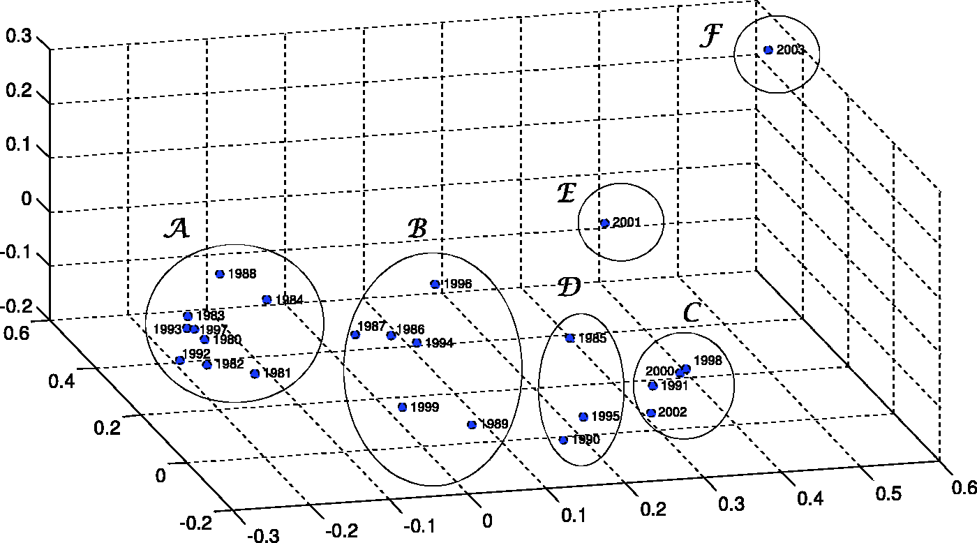

5. Conclusions

In this paper we proposed analyzing FFs from the perspective of dynamical systems. We used daily data for Portugal (excluding the Atlantic islands Azores and Madeira), covering the time period from 1980–2003. In the adopted methodology, burnt area, precipitation and atmospheric temperatures were interpreted as state variables of a CS and the correlations between them were investigated. First, we used the MI concept to unveil potential relationships in the data. Second, we considered the SSP to characterize the system’s behavior. Third, we compared the annual state space curves and adopted HC and MDS techniques to unveil existing patterns. Both tools identified the same clusters and exposed similarities between groups of consecutive years. The proposed analysis and findings can further contribute to better understand FF behavior and reveal hidden features not captured by standard tools.

Footnotes

Acknowledgments

The authors acknowledge the Instituto da Conservação da Natureza e das Florestas (INCF), the Instituto Português do Mar e da Atmosfera (IPMA) and the National Aeronautics and Space Administration (NASA) for the data.

Funding

The author(s) received no financial support for the research, authorship, and/or publication of this article.

References

Alvarado E, Sandberg DV and Pickford SG (1998) Modeling large forest fires as extreme events. Northwest Science 72: 66–75.

Bak

(1990) Self-organized criticality. Physica A: Statistical Mechanics and its Applications 163(1): 403–409.

Belo-Pereira

Dutra

Viterbo

(2011) Evaluation of global precipitation data sets over the Iberian Peninsula. Journal of Geophysical Research: Atmospheres 116: D20101.

Boer

Sadler

Bradstock

Gill

Grierson

(2008) Spatial scale invariance of southern Australian forest fires mirrors the scaling behaviour of fire-driving weather events. Landscape Ecology 23(8): 899–913.

Brooks

D'Antonio

Richardson

(2004) Effects of invasive alien plants on fire regimes. BioScience 54(7): 677–688.

Carlson

Doyle

(1999) Highly optimized tolerance: A mechanism for power laws in designed systems. Physical Review E 60(2): 1412.

Certini

(2005) Effects of fire on properties of forest soils: a review. Oecologia 143(1): 1–10.

Chandler

Cheney

Thomas

(1983) Fire in Forestry, New York: John Wiley & Sons.

Cox

(2000) Multidimensional Scaling, Boca Raton: CRC Press.

10.

Dale

(2001) Climate change and forest disturbances: Climate change can affect forests by altering the frequency, intensity, duration, and timing of fire, drought, introduced species, insect and pathogen outbreaks, hurricanes, windstorms, ice storms, or landslides. BioScience 51(9): 723–734.

11.

Drossel

Schwabl

(1992) Self-organized critical forest-fire model. Physical Review Letters 69(11): 1629.

12.

Flannigan

Stocks

Wotton

(2000) Climate change and forest fires. Science of the Total Environment 262(3): 221–229.

13.

Fraser

Swinney

(1986) Independent coordinates for strange attractors from mutual information. Physical Review A 33(2): 1134.

14.

Grassberger

Kantz

(1991) On a forest fire model with supposed self-organized criticality. Journal of Statistical Physics 63(3–4): 685–700.

15.

Hartigan

(1975) Clustering Algorithms, New York: John Wiley & Sons.

16.

Holmes

Huggett

Westerling

(2008) Statistical analysis of large wildfires. In: The Economics of Forest Disturbances, Netherlands: Springer, pp. 59–77.

17.

Jain

(2010) Data clustering: 50 years beyond K-means. Pattern Recognition Letters 31(8): 651–666.

18.

Kirilenko

Sedjo

(2007) Climate change impacts on forestry. Proceedings of the National Academy of Sciences of the United States of America 104(50): 19697–19702.

19.

Lasaponara

Santulli

Telesca

(2005) Time-clustering analysis of forest-fire sequences in southern Italy. Chaos, Solitons & Fractals 24(1): 139–149.

20.

Logan

Regniere

Powell

(2003) Assessing the impacts of global warming on forest pest dynamics. Frontiers in Ecology and the Environment 1(3): 130–137.

21.

Lopes

Tenreiro Machado

(2014) Analysis of temperature time-series: Embedding dynamics into the MDS method. Communications in Nonlinear Science and Numerical Simulation 19(4): 851–871.

22.

Malamud

Morein

Turcotte

(1998) Forest fires: An example of self-organized critical behavior. Science 281(5384): 1840–1842.

23.

Matsuda

(2000) Physical nature of higher-order mutual information: Intrinsic correlations and frustration. Physical Review E 62(3): 3096.

24.

Moritz

(2005) Wildfires, complexity, and highly optimized tolerance. Proceedings of the National Academy of Sciences of the United States of America 102(50): 17912–17917.

25.

Page

(2002) The amount of carbon released from peat and forest fires in Indonesia during 1997. Nature 420(6911): 61–65.

26.

Polderman

Willems

(1998) Introduction to Mathematical Systems Theory: A Behavioral Approach, New York: Springer.

27.

Reed

McKelvey

(2002) Power-law behaviour and parametric models for the size-distribution of forest fires. Ecological Modelling 150(3): 239–254.

28.

Ricotta

Avena

Marchetti

(1999) The flaming sandpile: self-organized criticality and wildfires. Ecological Modelling 119(1): 73–77.

29.

Rittmaster

(2006) Economic analysis of health effects from forest fires. Canadian Journal of Forest Research 36(4): 868–877.

30.

Shannon

(2001) A mathematical theory of communication. Mobile Computing and Communications Review 5(1): 3–55.

31.

Smith JK, Lyon LJ, Huff M, et al. (2000) Wildland fire in ecosystems. Effects of fire on fauna. Report no. RMRS-GTR-42. Rocky Mountain Research Station: USDA Forest Service.

32.

Song

(2006) Three types of power-law distribution of forest fires in Japan. Ecological Modelling 196(3): 527–532.

33.

Telesca

(2005) Time-scaling properties in forest-fire sequences observed in Gargano area (southern Italy). Ecological Modelling 185(2): 531–544.

34.

Tenreiro Machado

Lopes

(2012) Dynamical analysis of the global warming. Mathematical Problems in Engineering 2012: 971641.

35.

Tenreiro Machado

Lopes

(2013) Analysis and visualization of seismic data using mutual information. Entropy 15(9): 3892–3909.

36.

Tenreiro Machado

Lopes

(2014) Analysis of forest fires by means of pseudo phase plane and multidimensional scaling methods. Mathematical Problems in Engineering 2014: 575872.

37.

Zheng

(2008) Detrended fluctuation analysis of forest fires and related weather parameters. Physica A: Statistical Mechanics and its Applications 387(8): 2091–2099.