Traditional diffusion tensor imaging (DTI) maps brain structure by fitting a diffusion model to the magnitude of the electrical signal acquired in magnetic resonance imaging (MRI). Fractional DTI employs anomalous diffusion models to obtain a better fit to real MRI data, which can exhibit anomalous diffusion in both time and space. In this paper, we describe the challenge of developing and employing anisotropic fractional diffusion models for DTI. Since anisotropy is clearly present in the three-dimensional MRI signal response, such models hold great promise for improving brain imaging. We then propose some candidate models, based on stochastic theory.
The structural complexity of the human brain is manifest at each level of functional organization: synapses, axons, neurons, cortical layers, fiber tracts, and cerebral convolutions (gyri and sulci) (Schaltenbrand and Wahren, 1998). Magnetic resonance imaging (MRI) in general, and diffusion tensor imaging (DTI) in particular, exhibit contrast that reflects tissue heterogeneity and anisotropy in both the white and the gray matter (Mori, 2006). The overall goal of these imaging modalities is to provide spatial maps of structural features that correspond to the specific neural networks that provide the basis for sensory awareness, memory, cognition and coordinated movement (Le Bihan, 1995). Disruption of these neural pathways is a hallmark of trauma, stroke, tumors and degenerative disease. Although MRI and DTI are useful clinical tools for diagnosis and treatment monitoring, their typical voxel resolution (1 mm3) is orders of magnitude above that of a single cell (10 µm3) (Johansen-Berg and Behrens, 2009). Therefore there is a need to probe sub-voxel structure to improve both the sensitivity and the specificity of diagnosis. Since water movement within the voxel leads to MR signal attenuation that reflects collisions with molecules, membranes, and axonal fibers (Haacke et al., 1999) we anticipate that stochastic models of diffusion (isotropic, anisotropic, restricted, hindered, Gaussian, nonGaussian) can be used to encode sub-millimeter structure.
2. Fractional DTI
The connection between diffusion and magnetic resonance for water protons is described by the Bloch–Torrey equation (Torrey, 1956; Haacke et al., 1999; Callaghan, 2011). Solving the Bloch–Torrey equation for an anisotropic material, such as brain white matter (WM), provides the basis for DTI (Le Bihan, 1995). In standard DTI, a pair of trapezoidal gradient pulses is added to the MR imaging sequence (Mori, 2006). The acquired diffusion-weighted (DW) signal S decays in a manner dependent upon the diffusion gradient strength, G, gradient duration, δ, and the time interval, Δ, between gradient pulses. The resultant decay can be modeled (Haacke et al., 1999) by the equation
where S0 is the initial signal intensity, γ is the gyromagnetic ratio (42.57 MHz/T for water protons), D is a symmetric positive-definite matrix that defines the diffusion tensor, G = Gg where g is a unit vector that points in the direction of the applied magnetic field gradient G. The eigenvector corresponding to the largest eigenvalue of the matrix D points in the direction of WM fibers, since the water is maximally dispersed in this direction. A single parameter b describes the overall diffusion sensitivity of a sequence, and for a pair of identical rectangular gradient pulses (height G and width δ) we find b = (γGδ)2(Δ − δ/3) (Haacke et al., 1999). Then (2.1) reduces to
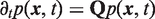
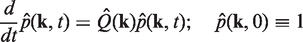
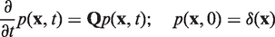
If the gradient pulses are of short duration (Callaghan, 2011), one can view (2.2) as the Fourier transform of the solution to a traditional diffusion equation, and this observation provides the essential link between MRI and diffusion: let p(x, t) be the probability density of a diffusing particle, which solves the diffusion equation
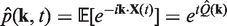
with a point source initial condition p(x, 0) = δ(x). Given a suitable function f(x), define its Fourier transform , and recall that is the Fourier transform of ∇f(x) (Meerschaert and Sikorskii, 2012, p. 150). Take Fourier transforms in (2.3) to get the ordinary differential equation with initial condition (k, 0) ≡ 1. Obviously the solution to this simple differential equation is p^(k, t) = exp(−tk · Dk), which is the same form as (2.2) with b = t‖k‖2 and g = k/‖k‖.
Since D is symmetric and positive definite, there is an orthonormal basis of eigenvectors v1, … , vd with corresponding eigenvalues ai such that Dvi = aivi for 1 ≤ i ≤ d. For any k ∈ ℝd we can write k = where kj = k · vj. Then vi · Dvj = 0 if j ≠ i and vi · Dvi = ai. It follows easily that
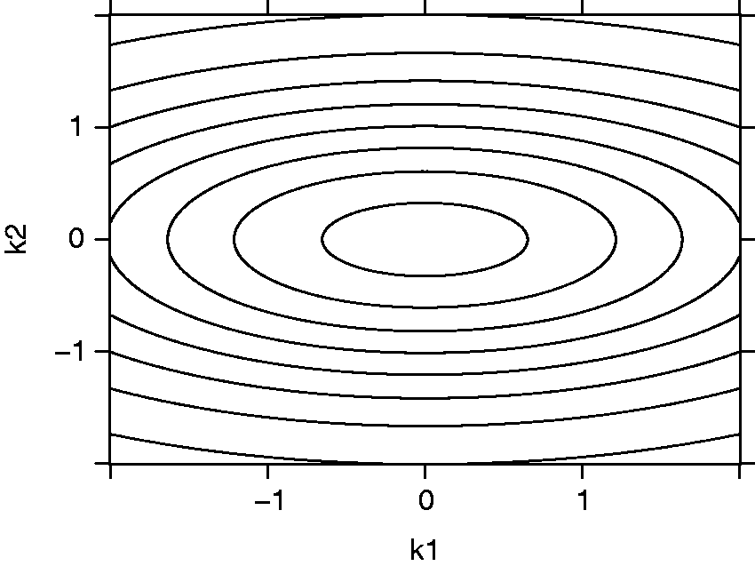
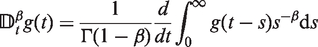
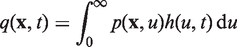
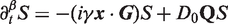
The level sets of the function are ellipsoids whose principal axes are the eigenvectors v1, … , vd. The level sets are widest in the direction of the eigenvector with the smallest eigenvalue. Figure 1 shows the level sets of this function at time t = 1 in the case where
in d = 2 dimensions. In this case, the eigenvectors of D are the coordinate axes, which give the major and minor axes of the elliptical level sets. As t increases, the level sets spread out at the rate t1/2, which is the hallmark of traditional diffusion. This spreading rate can easily be verified by noting that (k, t) = (t1/2k, 1). This solution exhibits mild isotropy, in which the solution spreading rate is radially symmetric, but the level sets are not. For complete details, see Meerschaert and Sikorskii (2012, Section 6.1).
Level sets of the Fourier solution (2.4) to the traditional diffusion equation in d = 2 dimensions with diffusion tensor (2.5) at b = 1.
In many applications (Metzler and Klafter, 2000, 2004; Mainardi, 2010; Meerschaert and Sikorskii, 2012), a diffusing front spreads at a different rate than the t1/2 predicted by the traditional diffusion equation. This can be captured by introducing fractional derivatives into the diffusion model. For simplicity, let us focus on the isotropic diffusion model where D = DI for some positive constant D, and where I is the d × d identity matrix. Then the diffusion equation (2.3) reduces to ∂tp(x, t) = DΔp(x, t), and its point source solution has Fourier transform (k, t) = exp(−Dt‖k‖2) where ‖k‖2 = k · k. The level sets of the solution p(x, t) are circles in two dimensions, or spheres in three dimensions.
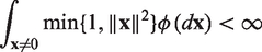
The fractional Laplacian is an isotropic space-fractional derivative, defined so that Δα/2f(x) has Fourier transform −‖k‖α(k) with 0 < α < 2. This reduces to the traditional Laplacian when α = 2. The isotropic space-fractional diffusion equation
has Fourier transform ∂tp^(k, t) = −D‖k‖α(k, t), whose point source solution is p^(k, t) = exp(−Dt‖k‖α). Since (k, t) = p^(t1/αk, 1), solutions spread like t1/α in this model, a phenomenon called superdiffusion. This model is also isotropic, which follows from the fact that p^(k, t) only depends on ‖k‖.
3. Fractional Bloch–Torrey equation
The traditional Bloch–Torrey equation
describes magnetization S(x, t) in a time-varying gradient G(t). Assume a solution S = S0Ae−ix·L where S0 > 0 is a constant, and A, L are functions of t with
Substitute the solution into (3.1) to see that
Compute ∇ · D∇S = L · DLS: then it follows that the solution with A(0) = 1 satisfies
for any t > 0. For a specified signal, it is then straightforward to compute the solution to the Bloch–Torrey equation (3.1). The Stejskal–Tanner pulse sequence consists of two rectangular functions of length δ separated by time Δ, with amplitude G and direction g. Then one can easily compute the solution (2.1), which reduces to (2.2) with b = (γGδ)2(Δ − δ/3).
The simplest space-fractional Bloch–Torrey equation
can be solved by a similar method. Assume the solution S = S0Ae−ix·L as before, and compute
Next compute the fractional Laplacian of the solution using Fourier transforms. It follows from the Fourier inversion formula f(x) = (2π)−d∫eik·x(k)dk that the function f(x) = e−ia·x has the Fourier transform f^(k) = (2π)dδ(k + a) using the Dirac delta function. Then D0Δα/2S is the inverse Fourier transform of −D0‖k‖αŜ(k, t), which is evidently −D0‖L‖αS. Hence we have
in this case. For a Stejskal–Tanner pulse sequence, the solution reduces to
where δ > 0 is a constant; see Magin et al. (2008) for more details. If we take D = D0Δ − D0(α − 1)δ/(α + 1) and b = γGδ, this reduces to the stretched exponential form
where 0 < α < 2.
4. The need for anisotropic fractional DTI models
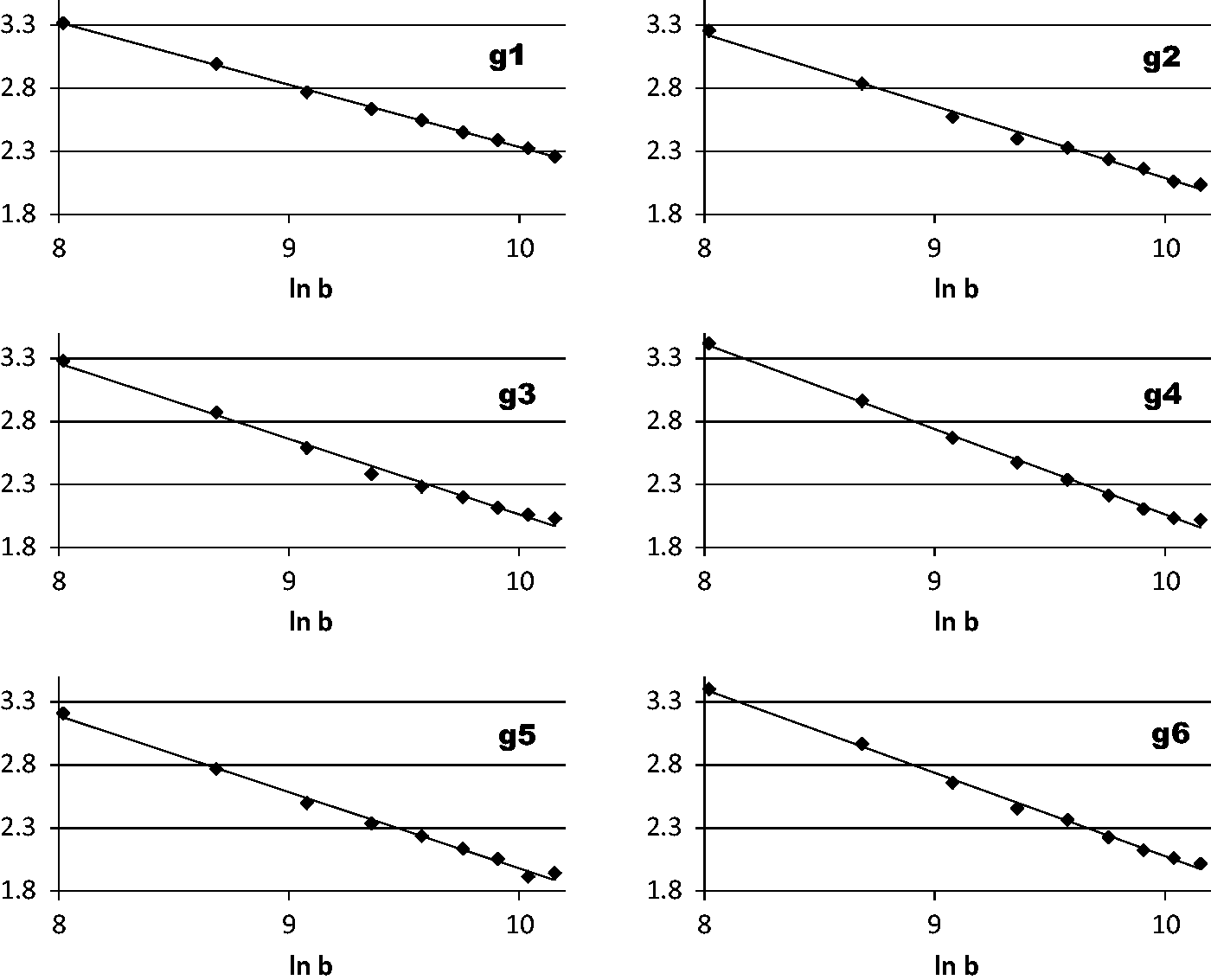
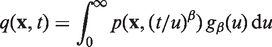
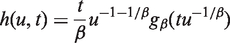
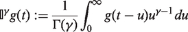
In MRI experiments, it is often observed (Bennett et al., 2003; Hall and Barrick, 2008; Ingo et al., 2014) that the acquired DW signal S follows the stretched exponential model (3.4) for high b values. In applications to brain imaging, it is also found that the parameter α varies with direction: an indication of anisotropy (Hall and Barrick, 2012). For example, in one experiment (Ingo et al., 2014), formalin-fixed brains from normal, adult rats were soaked in Fluorinert to reduce magnetic susceptibility and imaged ex vivo in a Bruker 750 MHz spectrometer (17.6 T, 89 mm bore). A pulsed gradient stimulated echo diffusion sequence was used with pulse repetition time of 2 s, echo time of 28 ms, in-plane resolution of 190 µm and slice thickness of 1 mm. The signal S was acquired in six different vector directions g1 = (0, 0, 1)T, g2 = (0.89, 0, 0.45)T, g3 = (0.28, 0.09, 0.45)T, g4 = (−0.72, −0.53, 0.45)T, g5 = (0.28, −0.85, 0.45)T, and g6 = (−0.72, −0.53, 0.45)T with 10 different b values ranging up to a maximum value of 26,190 s/mm2. In this experiment, Δ (17.5 ms) and δ (3.5 ms) were kept constant and G was scaled to increase with the b value. Under these conditions, the short-pulse condition δ ≪Δ holds.
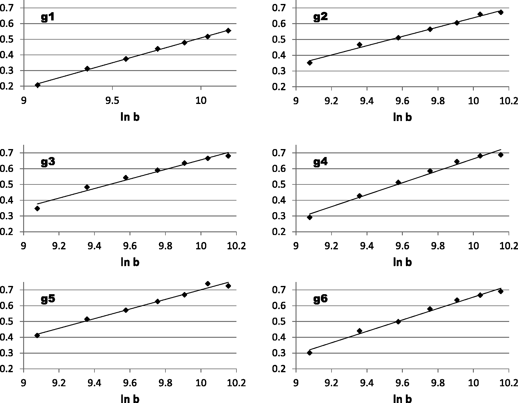
Next, we validate the stretched exponential model (3.4) using linear regression. Taking logs in the model yields ln(S/S0) = −Dbα, and taking logs again produces
Hence, a plot of s versus ln b should produce a straight line with slope α. Figure 2 shows this plot for each of the directions g1,… , g6 along with the best-fitting straight line model, found using simple linear regression. It is apparent from these graphs that the relation between the acquired signals S and b follows the stretched exponential model (3.4).
Plot of s versus ln b in six different directions, to validate the stretched exponential model (4.1).
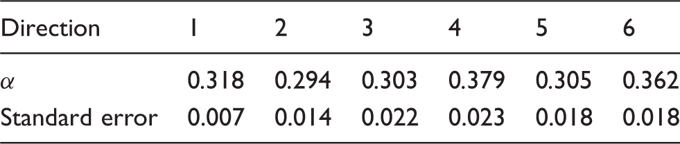
To illustrate the anisotropic nature of DTI, we compare the slopes α from the straight line fit of s versus ln b for each direction j = 1, 2, … , 6. The results are summarized in Table 1. It is clear that the power law slope depends on direction. For example, the slope for direction 4 (corresponding to direction vector g4) is α = 0.379 ±0.023 which is significantly different from the α = 0.294 value in direction 2. To obtain a formal confidence interval for these α values, one can use the standard t-interval from linear regression theory. Since the sample size is n = 7, the 95% confidence interval is α ± 2.571 SE where α is the estimate in the first row of Table 1, SE is the standard error in the second row of Table 1, and 2.571 is the 97.5th percentile of the standard t distribution with n − 2 = 5 degrees of freedom. For example, we are 95% confident that the correct α value for direction 1 lies in the interval (0.300, 0.336).
Best-fit α values via linear regression on the data in Figure 2 for six different directions, demonstrating anisotropy.
Direction
1
2
3
4
5
6
α
0.318
0.294
0.303
0.379
0.305
0.362
Standard error
0.007
0.014
0.022
0.023
0.018
0.018
Previous work has shown α to be a biomarker that reflects tissue heterogeneity (Bennett et al., 2003; Ozarslan and Mareci, 2003; Hall and Barrick, 2008; Magin et al., 2008; Zhou et al., 2010; Palombo et al., 2011; Ingo et al., 2014; Magin et al., 2014). In particular, the stretched exponential parameter α exhibits a lower value in more tortuous porous materials, and more heterogeneous tissue. Since the heterogeneity parameter α also varies with direction, it would be advantageous to include anisotropy in the fractional DTI model, to capture this effect.
5. Anisotropic fractional diffusion models for DTI
In the previous section, we demonstrated that the anisotropy parameter α in a DTI model can vary with direction. An open challenge in MRI theory is to develop a suitable anisotropic model for fractional diffusion that captures this anisotropy, and can be fit to data acquired within the constraints of a clinical MR scan. The scan generates multidimensional data that must be quickly and accurately presented to the radiologist for analysis. Fractional order models are attractive because they capture tissue complexity in a small set of parameters. Within the continuous time random walk (CTRW) paradigm, for example, the random motion of water is hindered or restricted by tissue heterogeneity that alters the waiting times and jump increments in a manner simply expressed by power laws (Metzler and Klafter, 2000, 2004; Meerschaert and Sikorskii, 2012). In the remainder of this paper, we survey existing anisotropic models for fractional DTI, and also discuss some potential new models.
5.1. Anisotropic fractional diffusion
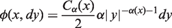
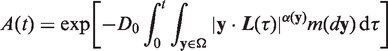
A recent paper of Hanyga and Magin (2014) proposed a new space-fractional diffusion model that seems well-suited for applications to DTI. The model is
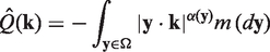
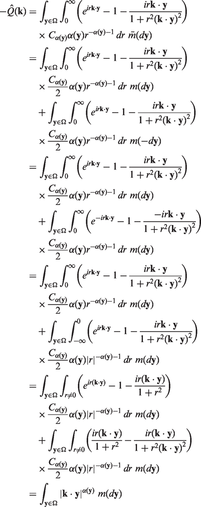
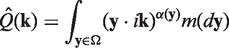
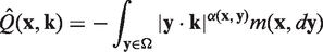
where the anisotropic fractional derivative operator Q is defined in terms of Fourier transforms. Define
where Ω = {y ∈ ℝd : ‖y‖ = 1} is the unit sphere in d-dimensional Euclidean space, m(dy) is a finite Borel measure on the sphere, and α(y) is a symmetric function α(y) = α(−y) on the sphere that takes values in the interval (0, 2). Then one defines Qf(x) to be the function with Fourier transform (k)f^(k). Hanyga and Magin (2014) continue to prove that solutions to (5.1) remain nonnegative for a nonnegative initial condition p(x, 0) = f(x) ≥ 0. Next we provide an alternative proof of this fact, by showing that the solutions to (5.1) are the probability densities of a Lévy process (Sato, 1999; Meerschaert and Sikorskii, 2012, Section 4.3).
Proposition 5.1
There exists a Lévy process X(t) that satisfies
for all k ∈ ℝd and all t ≥ 0, for any symmetric index function α: Ω → (0, 2) and any finite Borel measure m(dy) on the unit sphere.
Proof
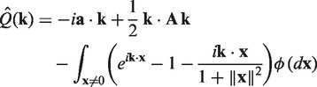
Any Lévy process {X(t) : t ≥ 0} is determined by the distribution of X: = X(1), which can be specified using the Lévy representation (Meerschaert and Scheffler, 2001, Theorem 3.1.11): a random vector X on ℝd is infinitely divisible if and only if we can write E[e−ik·X] = exp((k)), where
for a ∈ ℝd, A a nonnegative definite d × d matrix, and φ a σ-finite Borel measure on ℝd\{0} such that
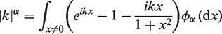
The triple [a, A, φ] is unique. Next we note that, in the one-dimensional case d = 1, there exists an infinitely divisible random variable X such that E[e−ikX] = exp(−|k|α) for any 0 < α < 2, and in this case, it follows from Meerschaert and Scheffler (2001, Lemma 7.3.10) (for 0 < α < 1), Meerschaert and Scheffler (2001, Lemma 7.3.11) (for 1 < α < 2), and Meerschaert and Scheffler (2001, Lemma 7.3.12) (for α = 1) that this random variable has Lévy representation [0, 0, φα] where
with
and C1 = 2/π. Then we have
for each 0 < α < 2. Next, define an infinitely divisible random vector X on ℝd (e.g. let d = 3) by specifying its Lévy representation [0, 0, φ] where x = ry in polar coordinates r > 0 and ‖y‖ = 1, and
where m(dy) = [m(dy) + m(−dy)]/2 is the symmetrized version of the measure m(dy). Then the random vector X has Lévy representation E[e−ik·X] = exp((k)), where
in view of (5.8), since the integral in the next to last line equals zero by symmetry. This shows that (5.3) holds. Since Cα is a bounded continuous function on the interval 0 < α < 2, it follows easily that (5.5) holds, so (5.9) is a Lévy measure.□
We say that a random vector X is full if it is not supported on a lower-dimensional hyperplane, that is, if there is no unit vector y ∈ Ω such that X · y = 0 with probability one.
Proposition 5.2
If ∫y∈Ω|y · w|α(y)m(dy) > 0 for every w ∈ Ω, and α(y) ≥ α0 > 0 for all y ∈ Ω, then the infinitely divisible random variable X(t) in Proposition 5.1 is full, and has a density p(x, t) with respect to Lebesgue measure for any t > 0.
Proof
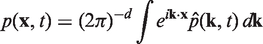
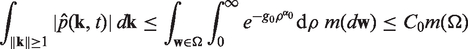
Define for all k ∈ ℝd and all t ≥ 0. The Fourier inversion theorem (Meerschaert and Scheffler, 2001, Theorem 1.3.7) implies that
is the function with Fourier transform (k, t), so long as the integral ∫|(k, t)|dk < ∞. Since (k) ≤ 0 for any k ∈ ℝd, it follows that 0 ≤ (k, t) ≤ 1 for all k ∈ ℝd and all t ≥ 0. Hence it suffices to check that ∫‖k‖ ≥ 1|(k, t)|dk < ∞. Adopt the polar coordinates k = ρw where ρ > 0 and ‖w‖ = 1. Since α(y) ≥ α0 > 0 for all y ∈ Ω, we have
for all ‖k‖ ≥ 1. It follows from the Dominated Convergence Theorem (Rudin, 1976, Theorem 11.32) that g(w) := ∫ y∈Ω|y · w|α(y)m(dy) is a continuous function on the compact set Ω, and since g(w) > 0 by assumption, it follows that g(w) ≥ g0 > 0 for all w ∈ Ω. Then − for all ‖k‖ ≥ 1. Then we have
where . This shows that (5.11) holds. If X(t) were not full, then we would have X(t) · w = 0 for some unit vector w, and then we would have E(e−iw·X(t)) = et(w) = 1, hence (w) = 0. But this contradicts −(k) ≥ g0ρα0, and so X(t) is full for every t > 0.□
Remark 5.3
Since p(x, t) is a probability density for any t > 0, it follows that p(x, t) ≥ 0 for all x ∈ ℝd and all t > 0. With some additional work, it should be possible to show that p(x, t) > 0 for all x ∈ ℝd and all t > 0.
Remark 5.4
It should not be hard to extend these arguments to the asymmetric case
which reduces to the case (5.2) if the measure m(dy) is symmetric, that is, m(dy) = m(−dy). One just has to be a bit careful about the centering constants.
Remark 5.5
A variety of stable-like processes have been considered in the literature, but the process constructed in Proposition 5.1 seems new. Bass (1988) considers a stable-like process in one dimension with jump intensity
which behaves locally like an α-stable process whose index varies in space. Bass and Tang (2009) consider a d-dimensional stable-like process with jump intensity φ(x, dy) = A(x,y)‖y‖−α−ddy where A(x,y) > 0 is bounded away from zero and infinity. That model exhibits mild anisotropy, as opposed to the strong anisotropy in the Hanyga model. It would certainly be interesting to explore the mathematical properties of the Lévy process in Proposition 5.1 in more detail.
5.2. Anisotropic fractional Bloch–Torrey equation
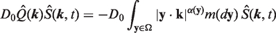
Here we propose a new anisotropic fractional Bloch–Torrey equation
which can be solved by the method introduced in Section 3. Assume the same solution form S = S0Ae−ix·L as before, and compute
Next compute S using Fourier transforms. Recall that the function f(x) = e−ia·x has Fourier transform =(2π)dδ(k + a). Then note that D0S has Fourier transform
Inverting as in Section 3, it follows that
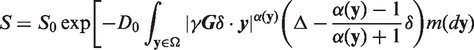
in this case. For a Stejskal–Tanner pulse sequence, the solution reduces to
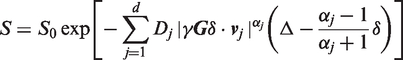
If the mixing measure m(dy) is concentrated on d point masses on an arbitrary set of coordinate axes v1, … , vd which need not be orthogonal, this reduces to a model recently proposed and tested by GadElkarim et al. (2013). That model has the solution
where Dj = D0m(vj), which agrees with GadElkarim et al. (2013, equation (20)) up to an obvious change in notation.
Remark 5.6
In practical applications, an open challenge is to fit the model (5.14) to MRI data as in Figure 2. The statistical problem is under-specified, since there are an infinite number of choices for α(y) and m(dy) = M(y)dy that will agree with any finite data set. One reasonable approach is to fit the simplest functions α(y) and M(y) using spherical harmonics in d = 3 dimensions. For example, the data in Figure 2 can be fit using six spherical harmonics. The resulting functions α(y) and M(y) will agree exactly with the measured values of α(y) and the corresponding weights M(y) obtained from the regression lines in Figure 2, and smoothly interpolate in between.
6. Time-fractional models for DTI
Here we explore the challenge of developing effective time-fractional models for DTI. These models can be useful if the data exhibit a power law decay in S as a function of b.
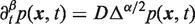
Anomalous subdiffusion can be modeled using a fractional derivative in time. Given a function f(t) with Laplace transform , recall that s˜f(s) − f(0) is the Laplace transform of the first derivative f′(s). The Caputo fractional derivative ∂tβf(t) is defined for 0 < β < 1 as the function with Laplace transform sβ(s) − sβ−1f(0), extending the traditional form. Take Fourier and then Laplace transforms in the space-time fractional diffusion equation
with point source initial condition (k, t) ≡ 0 to get sβ(k, s) − sβ−1 = −D‖k‖α(k, s), where (k, s) is the Laplace transform of (k, t). Solve to obtain
and then use the fact that (s): = sβ − 1/(sβ + c) is the Laplace transform of g(t) = Eβ(−ctβ), where the Mittag-Leffler function
for β > 0 (Mainardi, 2010, p. 223). It follows that p^(k, t) = Eβ(−tβD‖k‖α) is the Fourier transform of the solution to the isotropic time-fractional diffusion equation (6.1). Since p^(k, t) = p^(tβ/αk, 1), solutions spread at the subdiffusive rate tβ/2 in this model when α = 2. This model is isotropic, since p^(k, t) only depends on ‖k‖. Recalling the asymptotic property
(Mainardi, 2010, p. 215) we can see that p^(k, t) then falls off like t−β for large values of t.
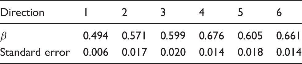
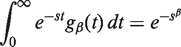
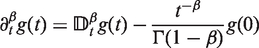
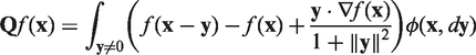
Figure 3 shows a log–log plot of S versus b for the data from Figure 2, for all six directions. The straight line behavior in Figure 3 shows that a time-fractional model is a reasonable alternative to the stretched exponential, since a power law S ≈ Cb−β also gives a good fit to the data. This is indicated by a straight line on the log–log plot with slope −β, since ln S ≈ ln C − β ln b. The β estimates and standard errors are listed in Table 2.
Plot of ln S versus ln b in six different directions, to validate the power law model S ≈ Cb−β.
Best-fit β values via linear regression on the data in Figure 3 for six different directions, demonstrating anisotropy.
Direction
1
2
3
4
5
6
β
0.494
0.571
0.599
0.676
0.605
0.661
Standard error
0.006
0.017
0.020
0.014
0.018
0.014
Again, it is clear that the data exhibit significant anisotropy, since the β values vary significantly with direction. For example, the value for direction 1 (corresponding to direction vector g1) is β = 0.494 ± 0.006 which is significantly different from the β = 0.571 value in direction 2. Since the sample size is n = 9, the 95% confidence interval is β ± 2.365 SE using the 97.5th percentile of the standard t distribution with n − 2 = 7 degrees of freedom. For example, we are 95% confident that the correct β value for direction 1 lies in the interval (0.480, 0.508).
6.1. Time-fractional Hanyga diffusion
The paper of Hanyga and Magin (2014) also proposed a time-fractional version of their anisotropic fractional diffusion model. Define the pseudo-differential operator on the space C0(ℝd) of smooth functions with compact support (i.e. f(x) = 0 for all ‖x‖ ≥ M for some M > 0) such that f(x) has Fourier transform (k)(k), where is defined by (5.2). This operator can then be extended to larger spaces of functions, or even distributions (i.e. generalized functions). Since , it is obvious that this Fourier transform solves the ordinary differential equation
Inverting the Fourier transform shows that the probability densities p(x, t) of the stochastic process X(t) from Proposition 5.1 solve the pseudo-differential equation
The equation (6.4) is also called a Cauchy problem (Arendt et al., 2001). In fact, if we define the semigroup
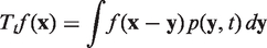
on the space L1(ℝd) of integrable functions f: ℝd → ℝ, then is the generator of that semigroup (Baeumer and Meerschaert, 2001, Theorem 2.2), and Ttf(x) solves the Cauchy problem
for any f ∈ Dom(), the domain of the generator. It follows from Baeumer and Meerschaert (2001, Proposition 2.1) that this semigroup Tt is strongly continuous and uniformly bounded, and that we can write the generator explicitly in the form
for any f ∈ W2,1(ℝd), the Sobolev space of functions in L1(ℝd) whose first and second partial derivatives are all in L1(ℝd).
Given any 0 < β < 1, define the Riemann–Liouville fractional derivative
Then it follows from Baeumer and Meerschaert (2001, Theorem 3.1) that the function
solves the fractional Cauchy problem
whenever p(x, t) solves the Cauchy problem (6.5). Here gβ(u) is the probability density function of the standard β-stable subordinator, most simply characterized in terms of its Laplace transform
for all s > 0, for any 0 < β < 1. A simple change of variable in the formula (6.6) reveals that
where
and this leads to a stochastic solution: let D(t) be the standard β-stable subordinator, a strictly increasing infinitely divisible Lévy process such that D = D(1) has the probability density function gβ(t). Define the inverse stable process (first passage time)
and apply Corollary 3.1 from Meerschaert and Scheffler (2004) to see that the function h(u,t) in (6.10) is the probability density function of the stochastic process Et for each t > 0. Then it follows by a standard conditioning argument that the solution q(x, t) to the fractional Cauchy problem (6.7) with the point source initial condition f(x) = δ(x) is also the probability density function of the time-changed process X(Et), where Et is independent from X(t). For a general initial condition f(x) that is a probability density function, the solution q(x, t) to the fractional Cauchy problem (6.7) with initial condition f(x) is the probability density function of X0 + X(Et), where the initial particle location X0 has probability density function f(x). See Meerschaert and Scheffler (2008, Theorem 4.1 and Remark 4.6) for more details and extensions. Freely available R code to compute the function h(u,t) is available (Meerschaert and Sikorskii, 2012, Example 5.13) so that the solution (6.9) to the fractional Cauchy problem can be explicitly computed by numerically integrating the formula (6.9), once the probability density function p(x, t) has been computed.
The Caputo and Riemann–Liouville fractional derivatives are related by
Then clearly one can also write the fractional Cauchy problem in a more compact form:
This extends the results of Hanyga (2002) for the case where β(y) is a constant.
6.2. Time-fractional Bloch–Torrey equation
Let be the generator of some C0 semigroup (Arendt et al., 2001). The time-fractional Bloch–Torrey equation has been written in the literature as
but this form is not dimensionally correct, since the time units of ∂tβS are different to the units of the term ∂tS and, more importantly, the reaction term −(iγx · G)S.
Using an idea from Baeumer et al. (2005), we can write a dimensionally correct version of the time-fractional Bloch–Torrey equation as
Equivalently, we can write
where is the Riemann–Liouville fractional integral defined by
An alternative form is proposed by Haynga and Seredyńska (2012, equation (17)). An open challenge in the theory of DTI is to derive an analytical solution for a physically correct time-fractional Bloch–Torrey equation, suitable for clinical applications.
7. Space-variable fractional DTI models
In clinical practice, the parameters of the (fractional) Bloch–Torrey equation vary with location. Indeed, three-dimensional maps of the parameters are an important outcome of fractional DTI modeling; see for example GadElkarim et al. (2013). An open challenge is to develop the mathematical foundations of space-variable fractional DTI models. One promising approach is to use the theory of pseudo-differential operators (Schilling, 1998; Jacob, 2001). We can consider the Cauchy problem
where the pseudo-differential operator is defined in terms of the equation
Here the Lévy measure is generalized to a jump intensity φ(x, dy) that varies in space. Then, for example, one can consider the Hanyga diffusion model where (5.2) is replaced by
The extension to time-fractional forms follows along the same lines as in Section 6, using the general theory of time-fractional Cauchy problems.
Footnotes
Acknowledgments
We would like to thank Andrzej Hanyga and Hans-Peter Scheffler for useful discussions that significantly improved the paper. We would also like to acknowledge Carson Ingo, Luis Colon-Perez, William Triplett and Thomas H Mareci for conducting the ex vivo DTI experiments that acquired the data plotted in Figures 2 and 3. These experiments are fully described by .
Funding
Mark M Meerschaert was partially supported by the NSF (grant EAR-1344280) and the NIH (grant R01-EB012079). Allen Q Ye was supported by the NIH (grant TL1TR000049).
BassRF (1988) Occupation time densities for stable-like processes and other pure jump Markov processes. Stochastic Processes and their Applications29: 65–83.
5.
BassRFTangH (2009) The martingale problem for a class of stable-like processes. Stochastic Processes and their Applications119: 1144–1167.
6.
BennettEMSchmaindaKMBennettRT (2003) Characterization of continuously distributed cortical water diffusion rates with a stretched-exponential model. Magnetic Resonance in Medicine50: 727–734.
7.
CallaghanPT (2011) Translational Dynamics and Magnetic Resonance: Principles of Pulsed Gradient Spin Echo NMR, Oxford: Oxford University Press.
8.
GadElkarimJJMaginRLMeerschaertMM (2013) Directional behavior of anomalous diffusion expressed through a multi-dimensional fractionalization of the Bloch-Torrey equation. IEEE Journal on Emerging and Selected Topics in Circuits and Systems3: 432–441.
9.
HaackeEMBrownRWThompsonMR (1999) Magnetic Resonance Imaging: Physical Principles and Sequence Design, New York, NY: Wiley-Liss.
10.
HallMGBarrickTR (2008) From diffusion-weighted MRI to anomalous diffusion imaging. Magnetic Resonance in Medicine59: 447–455.
HanygaA (2002) Multi-dimensional solutions of space-time-fractional diffusion equations. Proceedings of the Royal Society of London A458(2018): 429–450.
13.
HanygaAMaginRL (2014) A new anisotropic fractional model of diffusion model in a bio-tissue for applications in diffusion tensor imaging. Proceedings of the Royal Society of London A470: 20140319.
14.
HanygaASeredyńskaM (2012) Anisotropy in high-resolution diffusion-weighted MRI and anomalous diffusion. Journal of Magnetic Resonance220: 85–93.
15.
IngoCMaginRLColon-PerezL (2014) On random walks and entropy in diffusion-weighted magnetic resonance imaging studies of neural tissue. Magnetic Resonance in Medicine71: 617–627.
16.
JacobN (2001) Pseudo Differential Operators and Markov ProcessesVol. I, London: Imperial College Press.
17.
Johansen-BergHBehrensTE (2009) Diffusion MRI: From Quantitative Measurement to In Vivo Neuroanatomy, London: Elsevier.
18.
Le BihanH (1995) Diffusion and Perfusion Magnetic Resonance Imaging: Applications to Functional MRI, New York, NY: Raven Press.
19.
MaginRLAbdullahOBaleanuD (2008) Anomalous diffusion expressed through fractional order differential operators in the Bloch–Torrey equation. Journal of Magnetic Resonance190(2): 255–270.
20.
MaginRLIngoCColon-PerezL (2014) Characterization of anomalous diffusion in porous biological tissues using fractional order derivatives and entropy. Microporous and Mesoporous Materials71: 617–627.
21.
MainardiF (2010) Fractional Calculus and Waves in Linear Viscoelasticity: An Introduction to Mathematical Models, Singapore: World Scientific.
22.
MeerschaertMMSchefflerHP (2001) Limit Distributions for Sums of Independent Random Vectors: Heavy Tails in Theory and Practice, Wiley: New York.
23.
MeerschaertMMSchefflerHP (2004) Limit theorems for continuous-time random walks with infinite mean waiting times. Journal of Applied Probability41: 623–638.
24.
MeerschaertMMSchefflerHP (2008) Triangular array limits for continuous time random walks. Stochastic Processes and their Applications118: 1606–1633.
25.
MeerschaertMMSikorskiiA (2012) Stochastic Models for Fractional Calculus, Berlin: De Gruyter.
26.
MetzlerRKlafterJ (2000) The random walk’s guide to anomalous diffusion: A fractional dynamics approach. Physics Reports339: 1–77.
27.
MetzlerRKlafterJ (2004) The restaurant at the end of the random walk: Recent developments in the description of anomalous transport by fractional dynamics. Journal of Physics A37: R161–R208.
28.
MoriS (2006) Introduction to Diffusion Tensor Imaging, Amsterdam: Elsevier.
29.
ÖzarslanEMareciTH (2003) Generalized diffusion tensor imaging and analytical relationships between diffusion tensor imaging and high angular resolution diffusion imaging. Magnetic Resonance in Medicine50: 955–965.
30.
PalomboMGabrielliADe SantisS (2011) Spatio-temporal anomalous diffusion in heterogeneous media by nuclear magnetic resonance. The Journal of Chemical Physics135(3): 034504.
31.
RudinW (1976) Principles of Mathematical Analysis, 3rd edn. New York, NY: McGraw-Hill.
32.
SatoKI (1999) Lévy Processes and Infinitely Divisible Distributions, Cambridge: Cambridge University Press.
33.
SchaltenbrandGWahrenH (1998) Atlas for Stereotaxy of the Human Brain, 2nd edn. Stuttgart, Germany: Thieme.
34.
SchillingRL (1998) Growth and Hölder conditions for the sample paths of Feller processes. Probability Theory and Related Fields112: 565–611.
35.
TorreyHC (1956) Bloch equations with diffusion terms. Physical Review104: 563–565.
36.
ZhouXJGaoQAbdullahO (2010) Studies of anomalous diffusion in the human brain using fractional order calculus. Magnetic Resonance in Medicine63: 562–569.