
Abstract
This paper reports two successive spectral collocation methods, that enable easy and highly accuracy discretization, for 1 + 1 and 2 + 1 fractional percolation equations (FPEs). The first step depends mainly on the shifted Legendre Gauss–Lobatto collocation method for spatial discretization. An expansion in a series of shifted Legendre polynomials for the approximate solution and its spatial derivatives occurring in the FPE is investigated. In addition, the Legendre-Gauss–Lobatto quadrature rule is established to treat the boundary conditions. Thereby, the expansion coefficients are then determined by reducing the FPE with its boundary conditions to a system of ordinary differential equations for these coefficients. The second step is to propose the shifted Chebyshev Gauss–Radau collocation scheme, for temporal discretization, to reduce such a system to a system of algebraic equations, which is far easier to solve. The proposed collocation scheme, both in temporal and spatial discretizations, is successfully extended to the numerical solution of two-dimensional FPEs. An upper bound of the absolute error is obtained of the approximate solution for the two-dimensional case. Convergence properties of the method are discussed through numerical examples. Several numerical examples with comparisons are reported to highlight the high accuracy of the present method over other numerical techniques.
Keywords
1. Introduction
Spectral methods (Heinrichs, 1989; Canuto et al., 2006; Doha et al., 2014b; Eslahchi et al., 2014; Kayedi-Bardeh et al., 2014; Khalil and Khan, 2014; Abdelkawy et al., 2015a) are often efficient and highly accurate schemes when compared with local methods. The speed of convergence is one of the great advantages of spectral approximations. The spectral collocation method is a specific type of spectral method that is more applicable and widely used to solve almost all types of differential equations (Bhrawy, 2014; Doha et al., 2014a; Bhrawy and Zaky, 2015b). In pseudo-spectral techniques for partial differential equations, the boundary conditions play a much more crucial role than for ordinary differential equations, and it becomes important to decide whether to satisfy the related conditions implicitly, in the formulation of the collocation scheme, or to investigate the related conditions as additional constraints. The boundary conditions were treated implicitly in some recent pseudo-spectral approximations (Bhrawy, 2014; Doha et al., 2014a).
The development and analysis of fractional calculus began in recent decades, when the fractional differential equation emerged as a tool for the description of phenomena in nature. Fractional differential equations (Giona and Roman, 1992; Kirchner et al., 2000; Magin, 2006; Li and Deng, 2007; Garrappa and Popolizio, 2011; Alipour et al., 2012; Baleanu et al., 2012; Machado et al., 2013; Rostamy et al., 2013) are used to model many phenomena in several fields (Pooseh et al., 2013; Dehghan et al., 2014; Lazo and Torres, 2014; Pinto and Carvalho, 2015; Raja and Chaudhary, 2015; Xu et al., 2015). Numerical techniques are widely used by scientists and engineers to solve fractional PDEs. A major advantage of numerical techniques is that a numerical solution can be obtained even when a problem has no analytical solution. In some cases, PDEs of fractional order can be solved analytically, where finding their solutions in the general case is hard and limited to the linear one. Therefore, there has been a growing interest in recent decades in developing numerical methods for solving FDEs. Several numerical treatments based on the improvement of finite difference schemes for FDEs are given in Meerschaert and Tadjeran (2006), Ding et al. (2010) and Wang and Du (2014). Also, efficient spectral algorithms (He, 1998; Chou et al., 2006; Chen et al., 2011b; Doha et al., 2011; Doha et al., 2012; Chen et al., 2013; Bhrawy, 2014; Bhrawy et al., 2015a; Chen et al., 2014; Irandoust-Pakchin et al., 2014; Abdelkawy et al., 2015b; Ezz-Eldien et al., 2015) have been designed and developed for solving different kinds of fractional differential equation.
Percolation flow problems (Chou et al., 2006) have been discussed in many fields including groundwater dynamics, seepage hydraulics, and fluid dynamics in porous media. He (1998) introduced analytical solutions for fractional percolation equations (FPEs) by using the variational iteration method. Fractional derivatives are becoming widely used and accepted in models of percolation flow problems. Recently, three advanced implicit finite difference methods have been investigated in Chen et al. (2011b, 2013, 2014) to discretize the numerical solutions of FPEs in one- and two-dimensional spaces. Along the same line of thought, Chen et al. (2011b) proposed a new implicit finite difference scheme for solving the 1 + 1 FPE. A developed numerical algorithm has been achieved and analyzed by Chen et al. (2013), for solving the 2 + 1 FPE. Several authors have also improved and developed efficient numerical methods for approximating the solution of other similar fractional PDEs (Chen et al., 2011a; Al-Khaled and Alquran, 2014; Irandoust-Pakchin et al., 2014; Mohebbi et al., 2014; Bhrawy and Zaky, 2015a; Bhrawy et al., 2015a, 2015b).
The main aim of the present paper is to propose a numerical method that improves the accuracy of the numerical solutions of FPEs in one- and two-dimensional space. The main advantage of the present method is that it proposes a collocation scheme for both temporal and spatial discretizations. Firstly, the shifted Legendre Gauss–Lobatto collocation (SL-GL-C) is proposed, with a suitable modification for treating the boundary conditions, for spatial discretization. This treatment, for the conditions, improves the accuracy of the scheme greatly. Therefore, the FPE with its boundary conditions is reduced to a system of ordinary differential equations (SODEs) subject to a vector of initial values. Secondly, the SC-GR-C is then investigated for temporal discretization, which is more reasonable for solving initial value problems. Thereby, the problem is reduced to a system of algebraic equations which makes it far easier to solve. In addition, this algorithm is developed for the numerical solution of FPEs in two dimensions. An upper bound of the absolute error is obtained for the approximate solution for the two-dimensional case. Finally, several numerical examples with comparisons highlighting the high accuracy and effectiveness of the present method are included. By choosing relatively limited Legendre Gauss–Lobatto and Chebyshev Gauss–Radau collocation nodes, we are able to obtain highly accurate solutions, confirming the applicability and high accuracy of the proposed method over other numerical schemes in the literature.
This article is organized as follows. Section 2 presents some fractional calculus preliminaries, and shifted Legendre and shifted Chebyshev polynomials. Spectral approximation schemes of 1 + 1 and 2 + 1 FPEs based on a combination of SL-GL-C and SC-GR-C methods are presented in Sections 3 and 4, respectively. Numerical results are introduced in Section 5. Finally, we end the paper with some concluding remarks.
2. Preliminaries and notation
This section presents several useful fractional definitions, and shifted Legendre and shifted Chebyshev polynomials.
2.1. Fractional calculus
There are many definitions of the fractional-order derivative, which are not necessarily equivalent to each other (Miller and Ross, 1993; Kayedi-Bardeh et al., 2014; Ezz-Eldien et al., 2015; Jafari and Tajadodi, 2015). Riemann–Liouville and Caputo fractional definitions are the two most popular definitions from all the other definitions of fractional calculus which have been introduced recently.
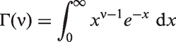
Definition 2.1
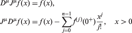
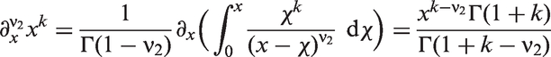
The Riemann–Liouville fractional integral of order ν ≥ 0 is obtained from
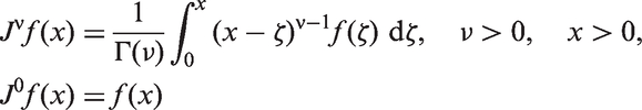
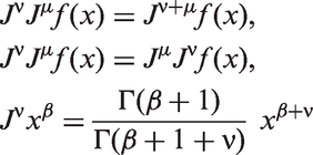
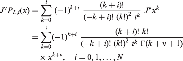
The fractional operator Jν satisfies
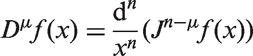
Lemma 2.1
If n − 1 < μ ≤ n, n ∈ N, then
2.2. Shifted Legendre Gauss–Lobatto interpolation
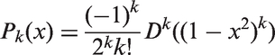
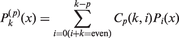
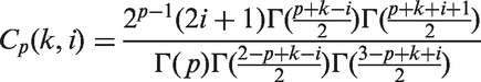
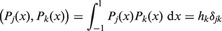
In this subsection, we recall some approximation results for the shifted Legendre Gauss–Lobatto (SL-GL) interpolation, which play important roles in the proposed collocation scheme. The Legendre polynomials P
k
(x) (k = 0,1…) satisfy the following Rodrigue's formula
For any positive integer N, let S
N
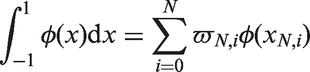
[ − 1,1] be the set of all polynomials of degree at most N, due to the L-GL quadrature. Thus, for any φ ∈ S2N−1[ − 1,1] we obtain
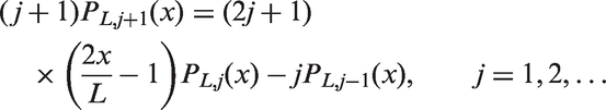
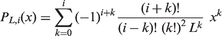
Let us denote by PL,i(x) the shifted Legendre polynomials which are defined on the interval [0,L]. These polynomials can be generated from the following recurrence relation
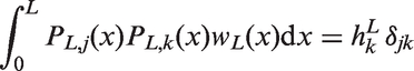
The orthogonality condition is
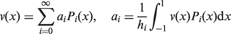
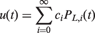
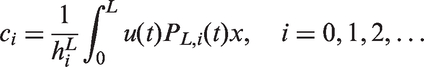
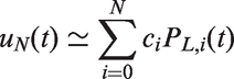
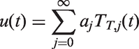
If a function u(t) ∈ L2[0,L], then one can express it by means of PL,i(t) as
2.3. Shifted Chebyshev Gauss–Radau interpolation
The Chebyshev polynomials are defined on the interval [ − 1,1], by


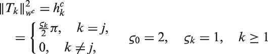
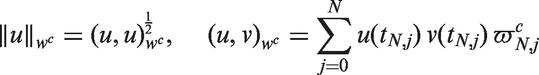
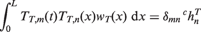
Let us denote by TT,n(t) the shifted Chebyshev polynomials which are defined on the interval [0,T]. The analytical form of TT,n(t) is obtained from
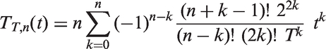
The orthogonality condition is
As in the previous subsection, if
3. One-dimensional space fractional percolation equation
This section outlines the key aspects of discretization for the numerical solution of the one-dimensional FPE using a new spectral technique.
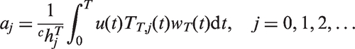
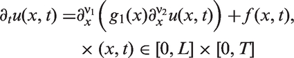
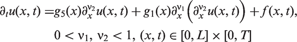
Consider the following 1 + 1 FPE


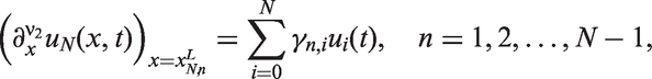
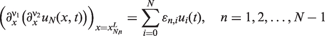
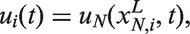
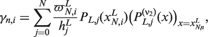
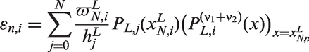
3.1. SL-GL-C scheme for the space variable
We first propose the SL-GL-C method to transform the 1 + 1 FPE into SODEs. To this end, we approximate the spatial variable using the SL-GL-C method at some nodes. The nodes are the set of points in a specified domain. To acquire high accuracy, the choice of nodes is usually related to some Gaussian integration formula, see Canuto et al. (2006) for more details. The collocation points are taken to be the SL-GL quadrature nodes which we denote by
Equation (27) may be restated as
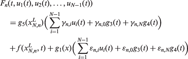
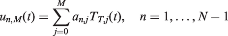
Now, we present the main steps of applying the SL-GL-C scheme to solve the FPE. Let the approximate solution of equation (27) be
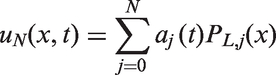
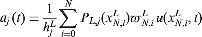
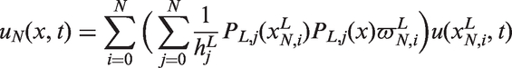
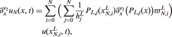
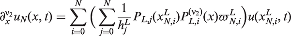
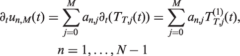
The fractional derivative of the approximate solution u
N
(x,t) is then estimated as
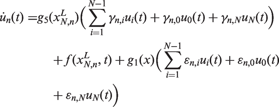
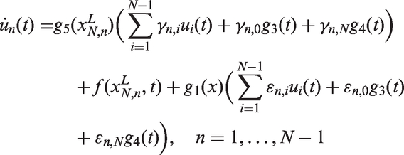

3.2. SC-GR-C scheme for the time variable
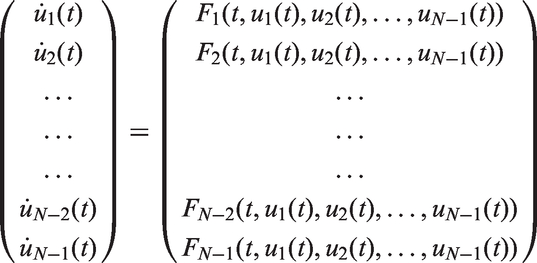
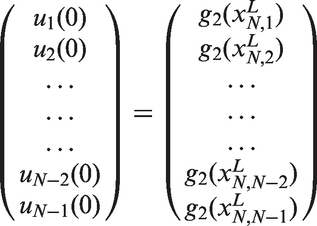
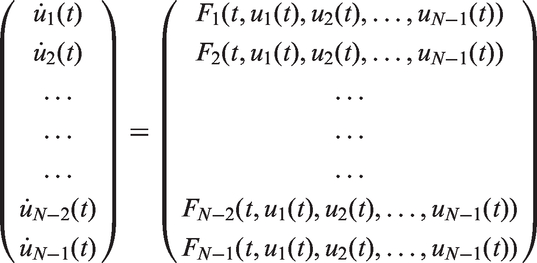
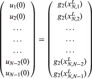
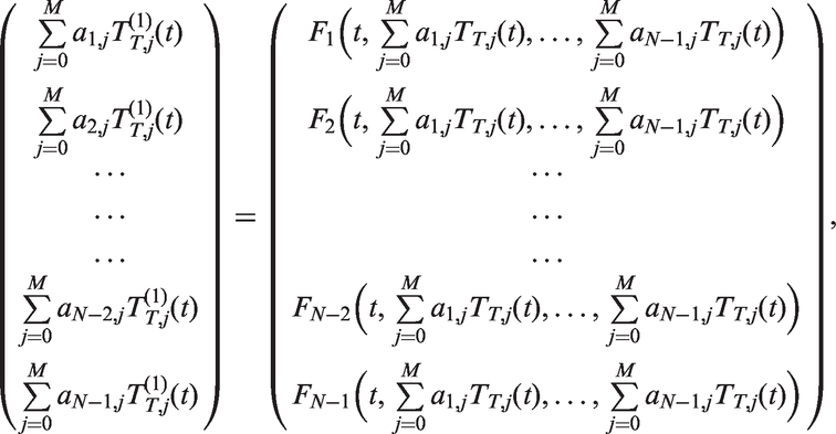
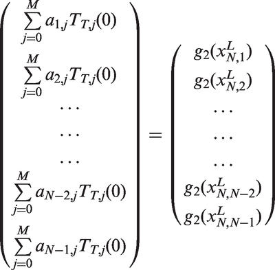
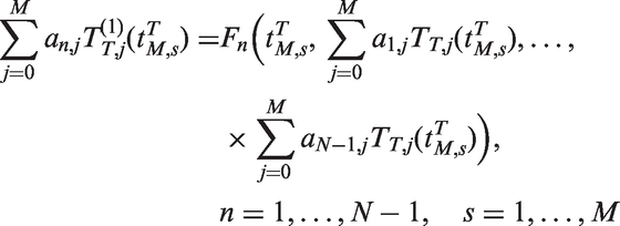
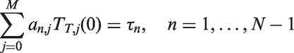
The second step of our algorithm is to propose an efficient collocation scheme to approximate the solution of the following SODEs
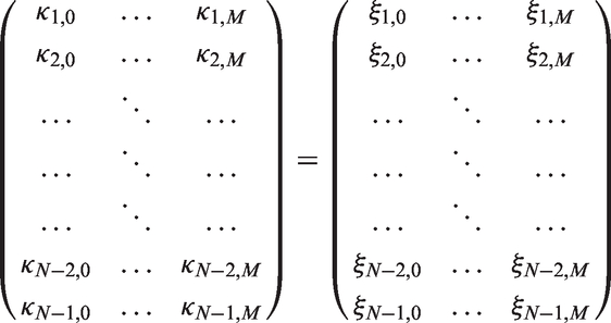
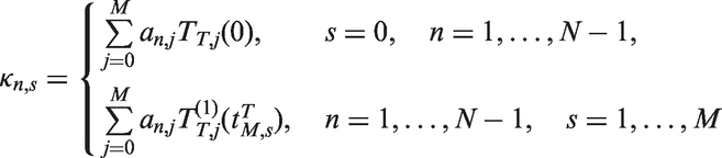
Therefore, adopting equations (49)–(50) enables one to write equations (47)–(48) in the form

4. Two-dimensional space fractional percolation equations
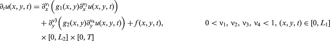
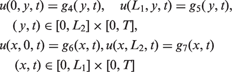
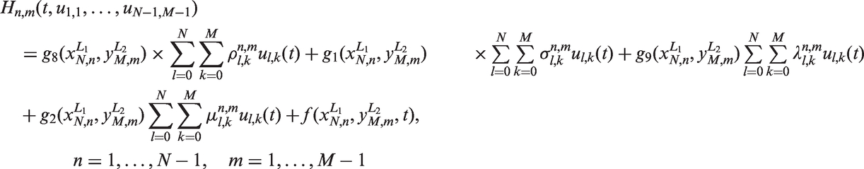
In this section, we develop the algorithm for one-dimensional FPEs to handle the following two-dimensional space FPE

4.1. SL-GL-C scheme for the space variable
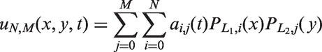
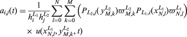
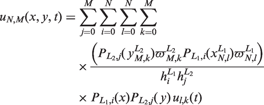
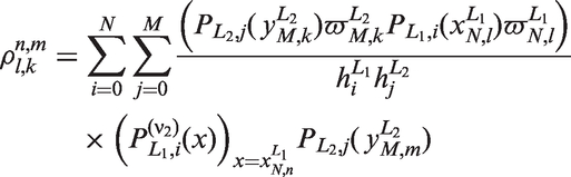
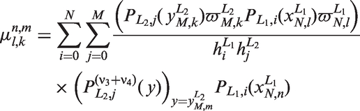
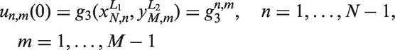
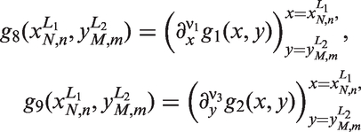
The SL-GL-C method will be extended to reduce the solution of the previous FPE into SODEs. Let us expand the dependent variable in the form
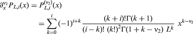
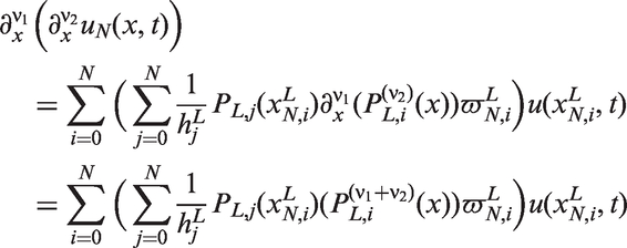
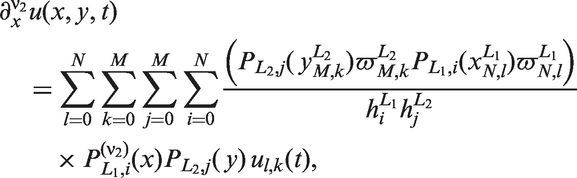
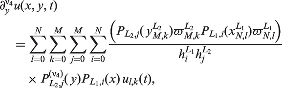
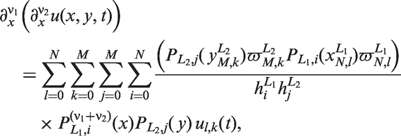
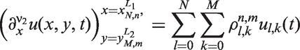
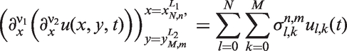
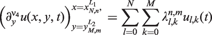
Similarly to equations (34)–(38), we compute the fractional spatial partial derivatives as


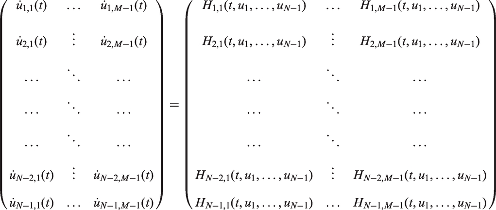
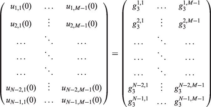
4.2. SC-GR-C scheme for the time variable
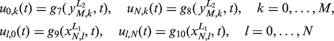
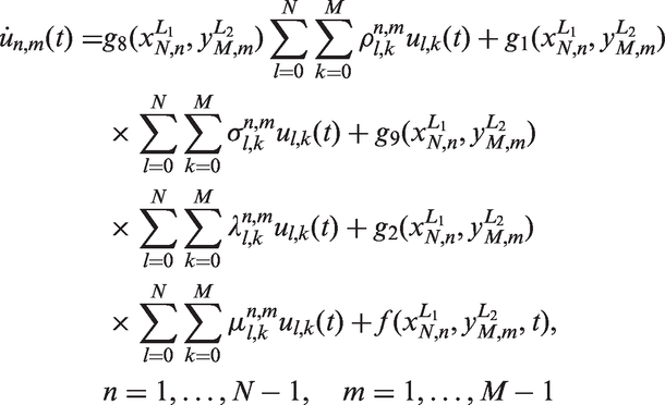
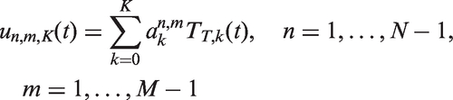
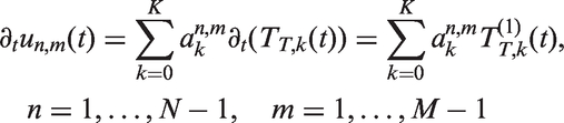
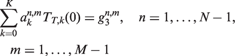
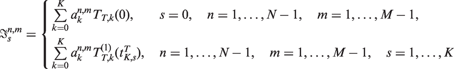
We are interested in using the SC-GR-C method to transform the SODEs (81) subject to equation (82) into a system of algebraic equations. To this end, we approximate the time variable using the following approximation
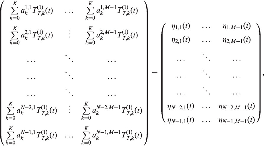
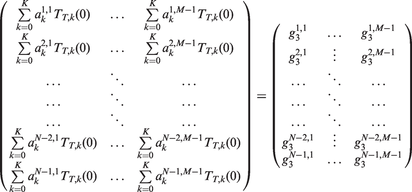
In the proposed method, the residual of equation (86) is set to be zero at K × (N − 1) × (M − 1) collocation points.


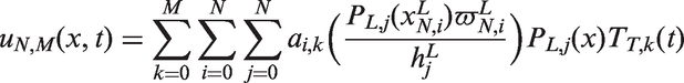
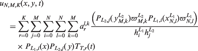
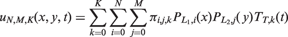
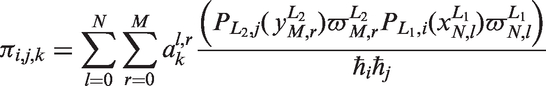
Finally, from equations (91)–(94), we get a system of (N − 1) × (M − 1) × (K + 1) algebraic equations. This system can be solved by any iteration technique. Then, the approximate solution uN,M,K(x,y,t) can be evaluated as
4.3. Error bound
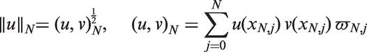
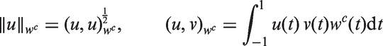
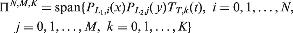
In this subsection, we present an analytic expression for the error norm of the best approximation for a smooth function u(x,y,t) ∈ Ω ≡ [0,L1] × [0,L2] × [0,T] by its expansion
Let us first consider the space
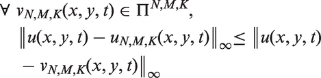
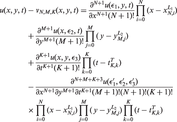

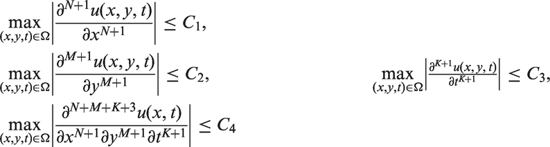
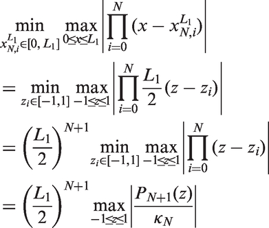

We can obtain
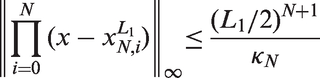
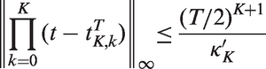
Combining equations (100), (101), (103) and (104), yields
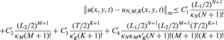
Hence, an upper bound of the absolute error is obtained for the approximate solutions. The convergence of the proposed method depends basically on the above error bound.
5. Numerical results and comparisons
After the construction of the spectral collocation methods, we now carry out some numerical examples of 1 + 1 and 2 + 1 FPEs to study the performance of the methods, which are discussed and developed in the current paper, and to compare our results with those proposed in Chen et al. (2011b, 2013, 2014). We divide this section into two main parts. In the first one, we introduce two examples of 1 + 1 FPEs. Then, we deal with three numerical examples of 2 + 1 FPEs in the second part.
5.1. Examples for one-dimensional space fractional percolation equations
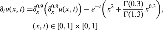
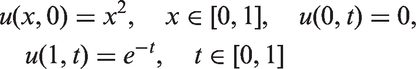
Example 1
Let us start with the following FPE (Chen et al., 2011b)

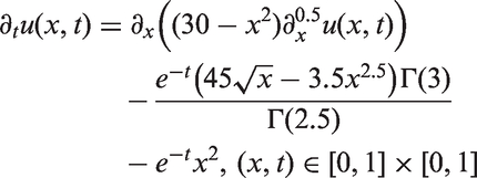
The exact solution is u(x,t) = e−t x2.
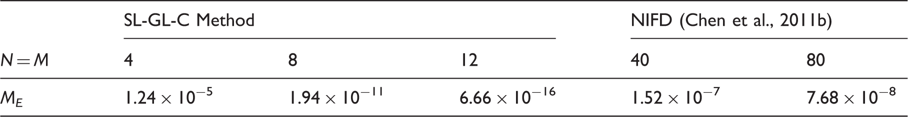
Comparing M E of the proposed method with the NIFD (Chen et al., 2011b) method for problem (106).
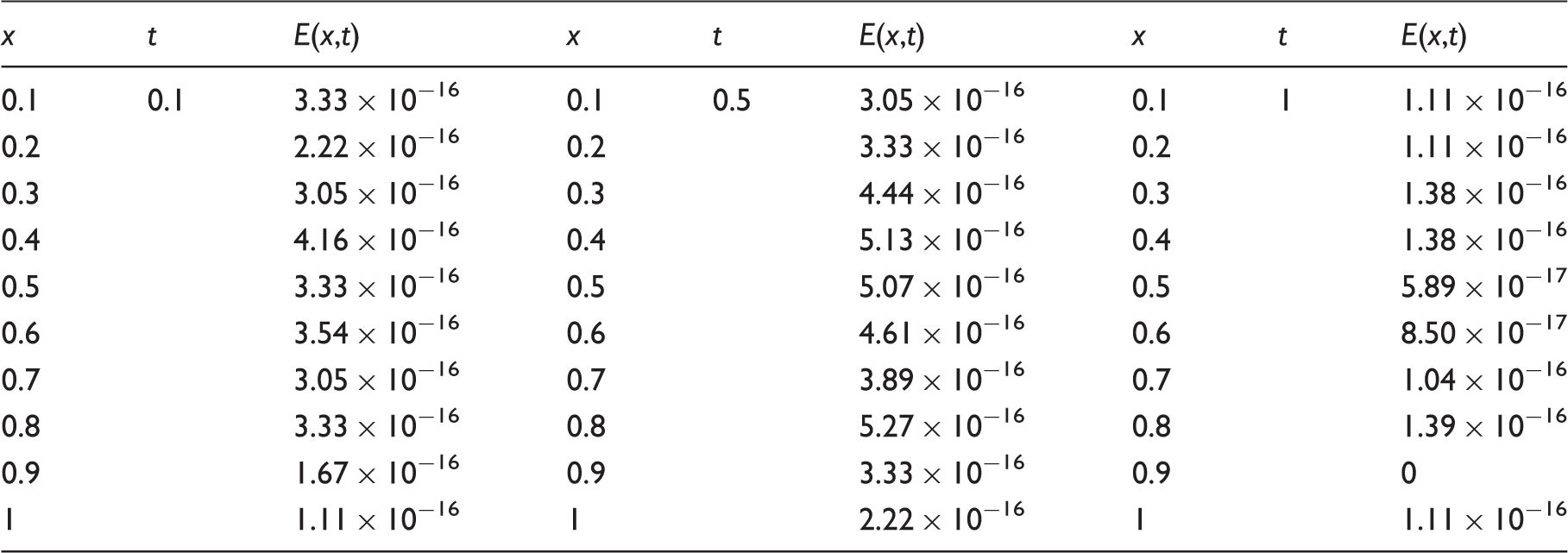
Absolute error at N = M = 12 and various choices of (x,t) for problem (106).
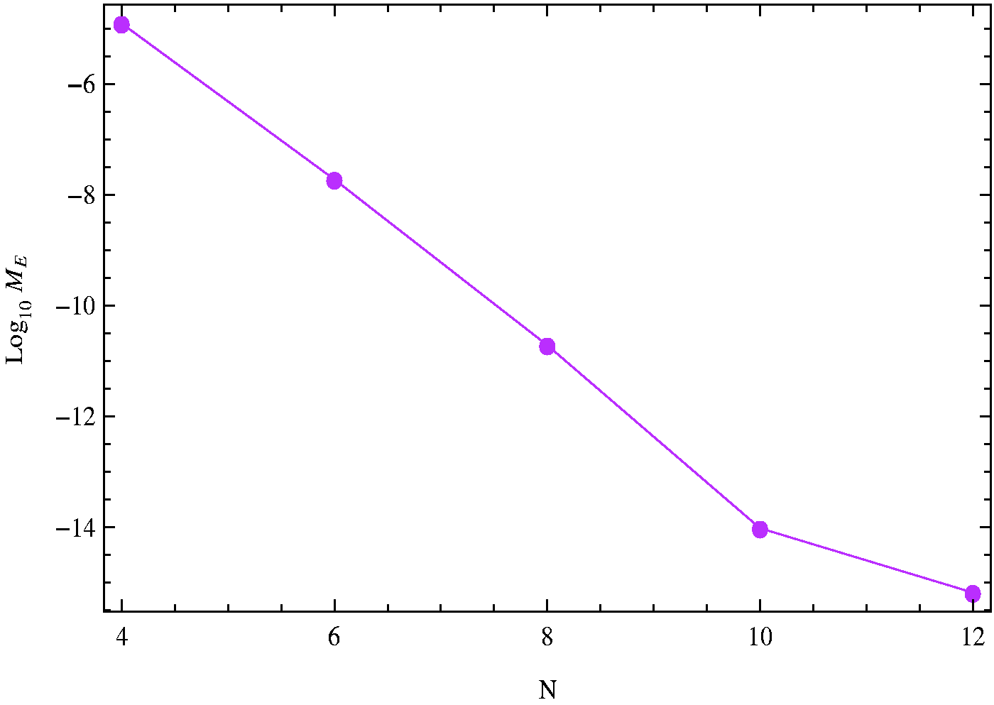
A space–time graph of the error function between the exact and approximate solutions at N = 12, is sketched in Figure 1. In addition, to confirm the high accuracy and convergence of the present scheme, in Figure 2, we plot the logarithmic graph of M
E
(log10 M
E
) at various values of N(N = M), which shows that the proposed method provides an accurate approximation and yields exponential convergence rates.
Absolute error of problem (106). Convergence of problem (106).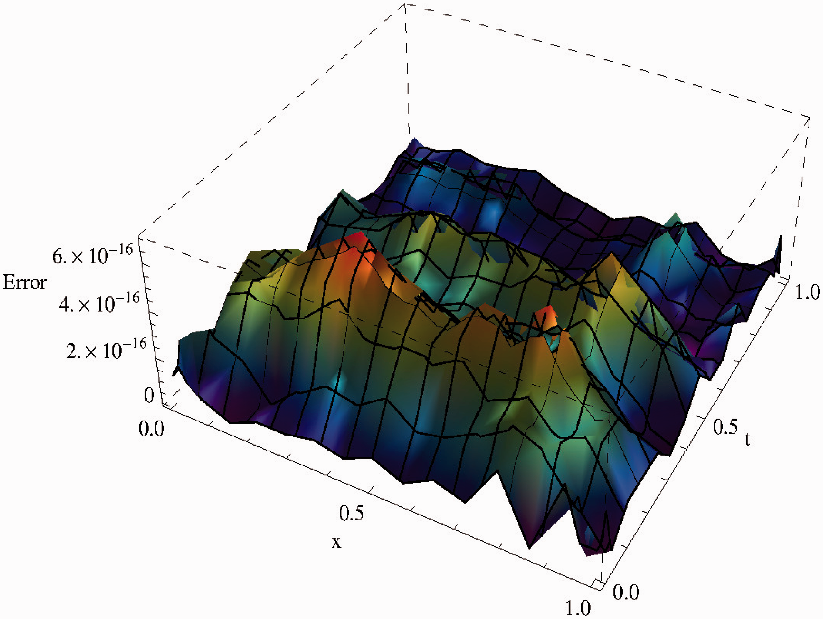
Example 2
Consider the following FPE (Chen et al., 2011b)
The exact solution is u(x,t) = e−t x2.
Comparing M E of the proposed method and the NIFD (Chen et al., 2011b) method for problem (108).
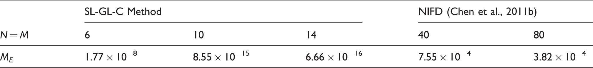
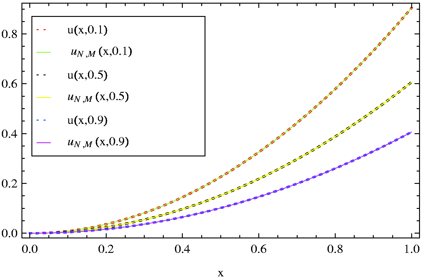
x-Directional curves of the approximate and exact solutions of problem (108) at N = M = 14.
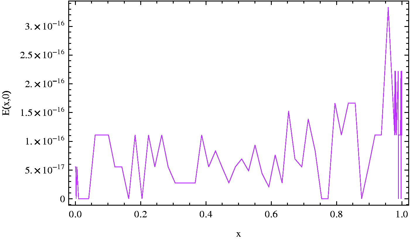
Absolute error of problem (108) at t = 0 and N = M = 14.
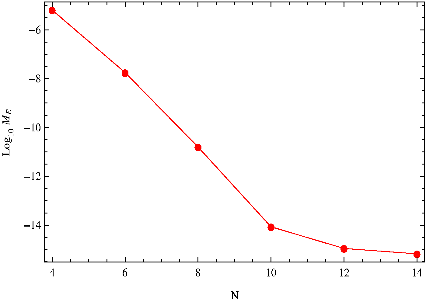
Convergence of problem (108).
5.2. Examples for two-dimensional space fractional percolation equations
Example 3
Consider the two-dimensional FPE (Chen et al., 2013)
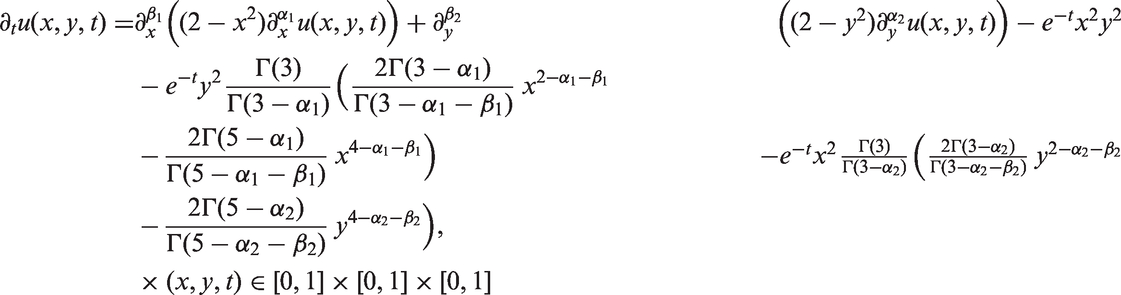


The exact solution is u(x,t) = e−t x2,y2.
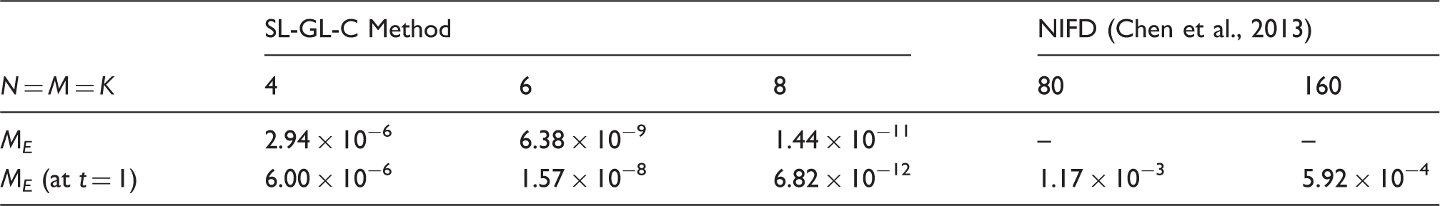
Comparing M E of the proposed method and the NIFD (Chen et al., 2013) method for problem (110) at α1 = 0.5, β1 = 1, α2 = 0.5 and β2 = 1.
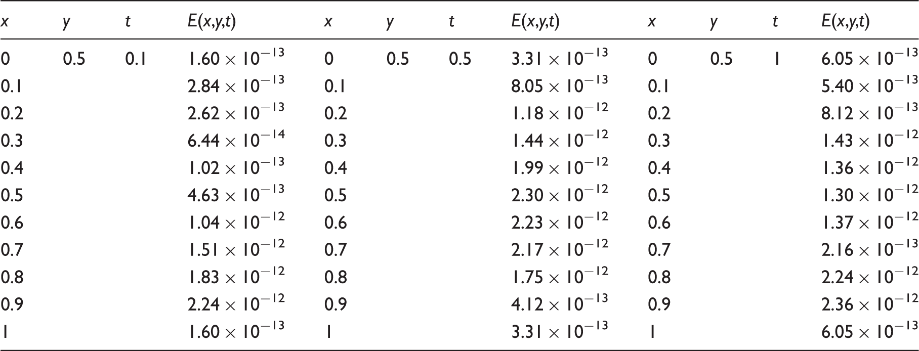
Absolute error for problem (110) with α1 = 0.5, β1 = 1, α2 = 0.5, β2 = 1 at N = M = K = 8.
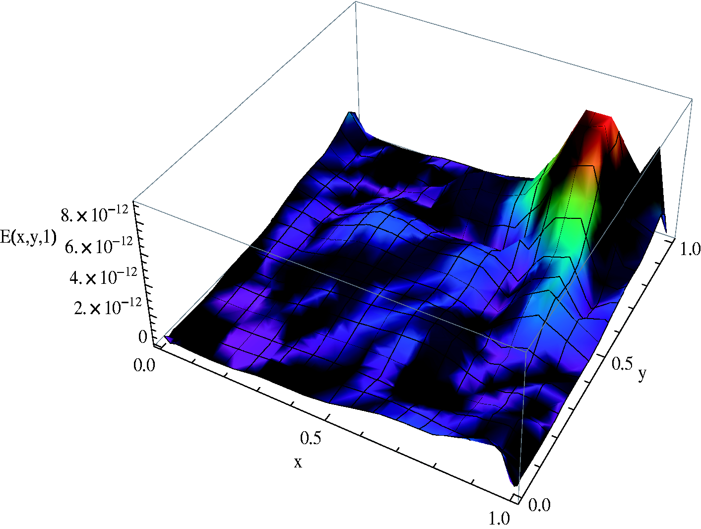
The space graph of the absolute error for problem (110) at α1 = 0.5, β1 = 1, α2 = 0.5, β2 = 1 and N = M = K = 8.
Convergence of problem (110).
Example 4
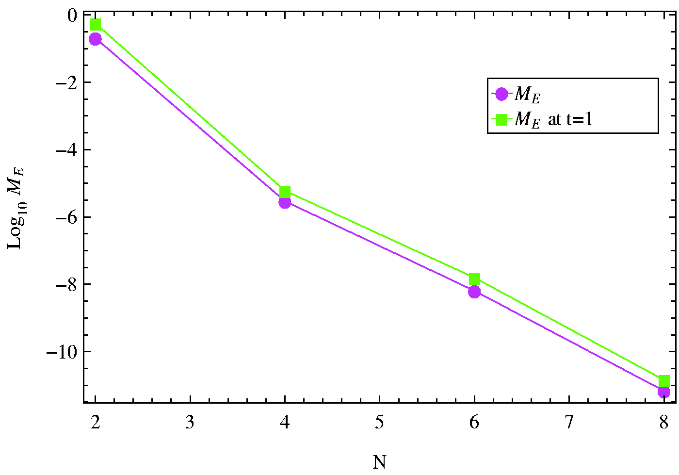
Consider the two-dimensional FPE (Chen et al., 2014)
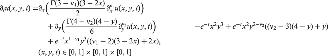


The exact solution of equation (113) is u(x,y,t) = e−t x2y3.
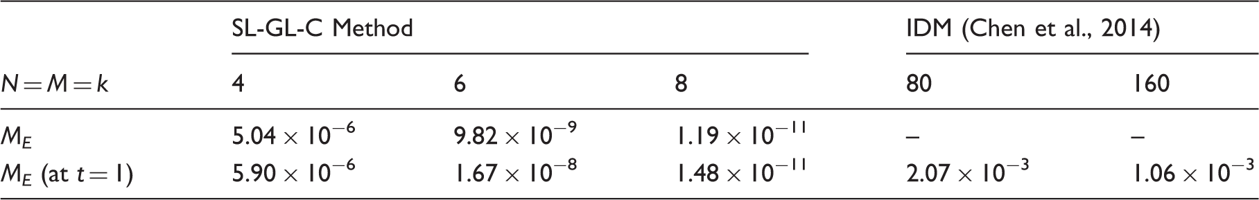
Comparing M E of the proposed method and IDM (Chen et al., 2014) for problem (113).
Example 5
Finally, consider the two-dimensional FPE
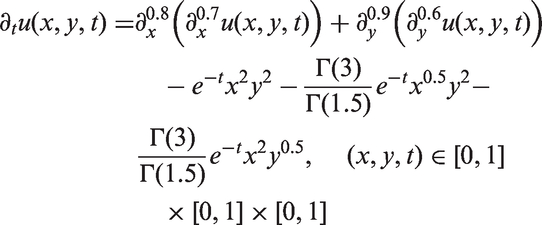

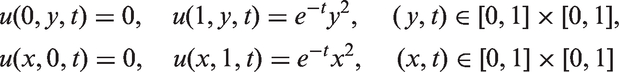
The exact solution of equation (116) is u(x,y,t) = e−t x2y2.
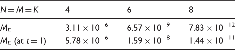
Maximum absolute error for problem (116).
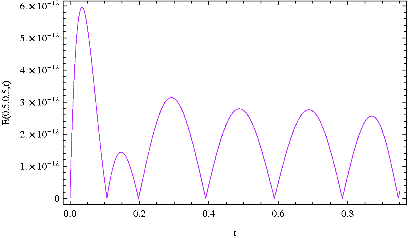
t-Directional curve of the absolute error of problem (116) at x = y = 0.5 and N = M = K = 8.
6. Conclusion
As one of the few articles dealing with FPEs, we have proposed and developed a spectral collocation method to obtain accurate numerical solutions for one- and two-dimensional FPEs. The core of the proposed method was to discretize the FPE in the spatial direction by the SL-GL-C method, along with a new treatment for the subjected conditions, to create SODEs of the unknown coefficients of spectral expansion in the time direction. An efficient numerical integration process for SODEs was investigated based on the SC-GR-C method. The proposed method has been successfully applied to numerically solve one- and two-dimensional FPEs. The main advantage of the present approach is, by adding a few terms of the shifted SL-GL and SC-GR collocation nodes, a highly accurate solution of the problem can be obtained. Comparison between our approximate solutions and the approximate solutions achieved by other methods were presented to demonstrate the high accuracy and validity of our method.
Footnotes
Acknowledgements
The authors are very grateful to the reviewers for carefully reading the paper and for their comments and suggestions which have improved the paper.
Funding
The author(s) received no financial support for the research, authorship, and/or publication of this article.