Receding horizon lateral vehicle control for pure pursuit path tracking

Abstract

The assimilation of path planning and motion control is a crucial capability for autonomous vehicles. Pure pursuit controllers are a prevalent class of path tracking algorithms for front wheel steering cars. Nonetheless, their performance is rather limited to relatively low speeds. In this paper, we propose a model predictive active yaw control implementation of pure pursuit path tracking that accommodates the vehicle’s steady state lateral dynamics to improve tracking performance at high speeds. A comparative numerical analysis was under taken between the proposed strategy and the traditional pure pursuit controller scheme. Tests were conducted for three different paths at iteratively increasing speeds from 1 m/s up to 20 m/s. The traditional pure pursuit controller was incapable of maintaining the vehicle stable at speeds upwards of 5m/s. The results show that implementing receding horizon strategy for pure pursuit tracking improves their performance. The contribution is apparent by preserving a relatively constant controller effort and consequently maintaining vehicle stability for speeds up to 100Km/h in different scenarios. A Matlab implementation of the proposed controller and datasets of the experimental paths are provided to supplement this work.

Keywords

Robotics Planning Control Path Autonomous Cars Path Tracking

1. Introduction

1.1. Autonomous vehicles

Cars are by far the most prevalent mode of transportation (Morris et al., 2013; Santos et al., 2011; Bureau of Transportation Statistics, 2013; Waldrop, 2015). The wide scale deployment of autonomous cars, fleets and transportation systems is expected to overcome the current limitations of vehicles, such as fuel efficiency, pollution, traffic congestion and accident risk (Laurgeau, 2012; Fagnant and Kockelman, 2014). Currently, the number of fatalities due to road accidents and collisions is estimated to be around 1.2 million per annum (Bureau of Infrastructure Transport and Regional Economics (BITRE), 2014; Bureau of Transportation Statistics, 2014). The majority of these accidents are attributed to unintended lane departure (Saleh et al., 2013), driver distraction (He et al., 2014), and human caused error (Lee, 2008). However, autonomous driving is still limited by various technological, infrastructural, economical and sociological factors. Passenger attitudes and public acceptance of self-driving are largely positive, as a result of the technological advancements and expected safety, economical and environmental benefits of autonomous cars (Preston, 2014; Payre et al., 2014; Schoettle and Sivak, 2014a, 2014b).

Advanced driver assistance systems (ADAS) are considered to be precursor technologies for autonomous driving. Intelligent transport systems are expected to keep shifting from driver assistance and shared control towards active safety and autonomous manoeuvring (Zheng, 2014; Bengler et al., 2014). Advancements in sensing, computing and robotics fields have enabled the development of autonomous vehicles. Early driver assistance systems were focused on lateral stability of vehicles, which is considered to be the main cause of accidents. Electronic Stability Controllers (ESC) combined yaw rate control with lateral acceleration, steering angle and wheel speed estimation to prevent instability of vehicles during manoeuvring (van Zanten, 1999; van Zanten, 2000). Satellite navigation systems are examples of technologies that contributed to driver safety by offering location and routing data to reduce driver distraction. ADAS have been proposed to reduce task loads on drivers and reduce driver performance degradation and distraction. For instance, forward warning collision systems and autonomous braking system were estimated to contribute to reducing accidents (Kusano and Gabler, 2012).

Autonomous passenger cars are vehicles that are capable of maneuvering roads independent of any driver control. The earliest research in autonomous driving in realistic environments is often traced back to early 1990’s at Carnegie Mellon University’s NavLab (Thorpe et al., 1991a, 1991b). The Defense Advanced Research Projects Agency (DARPA) Grand Challenges in 2003 and 2004 inspired research interest in autonomous driving technology. In 2007, the DARPA urban challenge took place in a controlled environment with a number of autonomous and human-operated cars. Ever since, a number of automotive manufacturers have announced self-driving cars research programs. It is expected that fully autonomous cars can be deployed on a consumer wide level in the upcoming years (NHTSA (National Highway Traffic Safety Administration), 2013). In that agenda, fully autonomous cars are expected to drive towards a desired destination without any expectation of shared control with driver, including safety critical tasks and unexpected changes in plans and layouts.

The operation of autonomous cars can be categorized into three stages, which are “Sense, Plan, and Act” also known as the SPA cycle. The initial sensing stage relies on using a number of sensors to describe the vehicle internal states (such as fuel level and location) and external surroundings (such as obstacles and roads). Vision and laser based sensing methods have been developed for developing maps of the surrounding environment and locating the vehicle and tracking pedestrians within that map (Geiger et al., 2013; Pandey et al., 2011). Particular sensing tasks for autonomous driving include using image processing for lane detection (Wang et al., 2004), and traffic light identification (Fairfield and Urmson, 2011). Based on the acquired information, the subsequent “plan” stage attempts to define a set of continuous actions to drive to the desired destination from a current estimated vehicle state. Incremental heuristics search and randomized search algorithms have been for vehicle path planning (Likhachev et al., 2008; Kuffner and LaValle, 2000; Elbanhawi and Simic, 2014). The final “act” stage defines controls commands in order to execute the desired plan, which is the focus of this paper. For autonomous cars, this is often referred to as path tracking control.

1.2. Path tracking controllers

Tracking reference trajectories for mobile robots is a fundamental problem in robotics. The motion of car-like robots is constrained. Consequently the ability for such vehicles to execute any trajectory is limited unlike wheeled mobile robots (see section 2). Several kinematic control laws were proposed for car like vehicles such as pure pursuit tracking (Craig, 1992), stanley controller (Thrun et al., 2007), critically damped controller (Cheein and Scaglia, 2013; Serrano et al., 2014), mixed controller (Lenain et al., 2009) and neural network (Gu and Hu, 2002). Pure pursuit controller is perhaps the most commonly used controller for car like tracking (Corke, 2011). The mixed controller used a kinematic control law with an side slip observer to account for wheel slip (Lenain et al., 2009). The controller proposed by Cheein and Scaglia (2013) outperformed pure pursuit and mixed controller in various simulations and field experiments. However, the critically damped controller has a does not allow for controlling the velocity of the vehicle. It is capable of bounding the velocity however when the velocity is fixed (for lateral control purposes) the controller oscillates and is rendered unstable. Snider (2009) conducted a comparative study between pure pursuit, Stanley, error based kinematic tracker and linear quadratic dynamic controller. Pure pursuit outperformed other controllers under stochastic actuation condition and discontinuous paths. These kinematic controllers were limited to low speed and small changes in steering as they ignore the dynamics of vehicle.

Model predictive control (MPC) manipulates the future control variable to optimise the predicted future plant performance. The optimized control and prediction timeframes are set to particular windows referred to as control and prediction horizons. Receding Horizon Control (RHC) is an iterative strategy of implementing the first step of the control horizon, revaluating the plant state and then recalculating the optimal control. Aripin et al. (2014) reviewed different controllers used for lateral vehicle control. MPC has been particularly successful as a strategy to improve the performance of multivariate dynamic nonlinear control systems (Mayne, 2014; Wang, 2009). Gu and Hu (2006) used MPC for kinematic tracking of wheeled robots. Attia et al. (2014) proposed MPC for lateral guidance of an integrated lateral and longitudinal controller. MPC steering control has also been shown to improve the vehicle stability under challenging driving conditions (Falcone et al., 2007; Beal and Gerdes, 2013). These strategies however did not report a thorough analysis of the controller performance and vehicle stability under systematic changes of the path design and vehicle speed.

1.3. Contribution

In this paper, we present a RHC approach particularly for pure pursuit (PP) tracking algorithms. This strategy is proposed to overcome the low speed limitations of traditional PP control. Therefore, a steering controller that maintains the vehicle’s stability and tracking performance at higher speeds is detailed in this article. The performance of the controller and stability of the vehicle were assessed using the criteria presented in Roth and Batavia (2002) and Tondel and Johansen (2005).

2. Methodology

2.1. Front wheel steering vehicle model

2.1.1. Kinematics

A single track bicycle model is used to represent a front-wheel-steered vehicle. This model adequately describes the global motion of the vehicle (Campion et al., 1996; Jazar, 2008). This model is based on the assumption of small slip angles, no road gradient or bank angles, no load transfer and no rolling or pitching moment. Only the front wheel is steerable in this case. In order to use the bicycle model, it is assumed that the average steering for both sides of the vehicle is equivalent to the single track steering angle when negotiating a turn. The two front wheels are represented as a front single track steerable wheel and the two back wheels are presented as a single track back wheel.

The bicycle model illustrated in Figure 1, where x, y and θ describe the position and heading of the car with respect to the global reference frame measured from the rear axle, φ is the steering angle, L is the wheelbase, v is the traction velocity and β is the side slip angle. The discrete model is approximated by equation (1) where t is time and Δt time step. The steering angle is mechanically limited to φ_max, which constrains the path that could be followed. This limitation is often described using a path curvature, k, upper bound, k_max, as given in equation (2). The vehicle is underactuated, as a result of having three degrees of freedom i.e. pose (x, y, θ) and two controls, v and φ. This results in a nonholonomic constraint between the resultant velocity components v_x and v_y in global [G] x and y directions, respectively, as shown in equation (3).

{x_{i + 1} = x_{i} + v_{i} . \cos (θ_{i}) . Δ t y_{i + 1} = y_{i} + v_{i} . \sin (θ_{i}) . Δ t θ_{i + 1} = θ_{i} + v_{i} . \frac{\tan (φ_{i})}{L} . Δ t

(1a)

{x_{i + 1} = x_{i} + v_{i} . \cos (θ_{i} + β_{i}) . Δ t y_{i + 1} = y_{i} + v_{i} . \sin (θ_{i} + β_{i}) . Δ t θ_{i + 1} = θ_{i} + v_{i} . \frac{\tan (φ_{i})}{L} . Δ t

(1b)

k_{\max} = \frac{1}{ρ_{\min}} = \frac{\tan (φ_{\max})}{L}

(2)

v_{x} \sin θ - v_{y} \cos θ = 0

(3)

Figure 1.

Kinematic Bicycle model (blue) for front wheel steering car with respect to a global reference frame.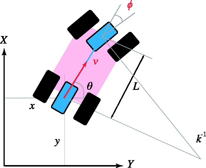

2.1.2. Lateral dynamics

The effects of suspension, steering, tires and mass distribution of the vehicle are not considered in path planning (Dolgov and Thrun, 2009; Ma et al., 2015). The bicycle model ignores dynamic effects of the vehicle and is limited to tracking paths at lower speeds and slip angles (Rajamani, 2012; Soudbakhsh and Eskandarian, 2012; Marzbani et al., 2015). For executing the planned reference paths at higher speed the tracking controller that must account for vehicle dynamics. This provides higher tracking accuracy and vehicle stability performance.

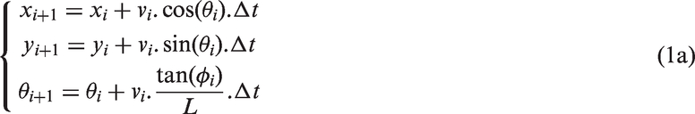
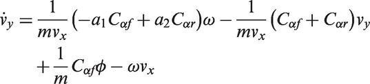
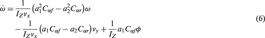
The equations of motion for the vehicle in reference to its mass centre are given in equations (4–6), where m is the mass of the vehicle. The front and rear distances from the mass centre are labelled as a₁ and a₂ in Figure 2. In this model the output are the longitudinal and lateral velocities, and the yaw rate, ω and the input is the steering angle. A linear tyre model is adopted for this model. Tyre coefficients C_αf and C_αr describe the relation between tyre lateral forces and wheel slip (Pacejka, 2006).

{\overset{\cdot}{v}}_{x} = \frac{F_{x}}{m} + ω v_{y}

(4)

{\overset{\cdot}{v}}_{y} = \frac{1}{{mv}_{x}} (- a_{1} C_{α f} + a_{2} C_{α r}) ω - \frac{1}{{mv}_{x}} (C_{α f} + C_{α r}) v_{y} + \frac{1}{m} C_{α f} φ - ω v_{x}

(5)

\overset{\cdot}{ω} = \frac{1}{I_{Z} v_{x}} (a_{1}^{2} C_{α f} - a_{2}^{2} C_{α r}) ω - \frac{1}{I_{Z} v_{x}} (a_{1} C_{α f} - a_{2} C_{α r}) v_{y} + \frac{1}{I_{Z}} a_{1} C_{α f} φ

(6)

Figure 2.

Vehicle lateral dynamic model and parameters.

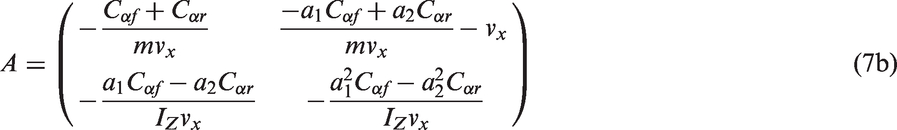
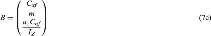
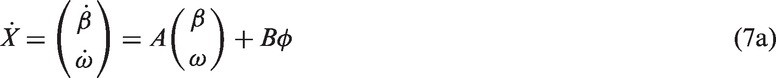
For lateral vehicle control, a fixed forward velocity is assumed allowing for an analytically solvable model (Pacejka, 2006; Soudbakhsh and Eskandarian, 2012; Attia et al., 2014; Marzbani et al., 2015). This enables the formulation of a two-degree of freedom time invariant linear model, given in equations (7) and (8). This assumption for constant velocity is valid for lateral control. In cases of variable speed driving, longitudinal control systems and cruise control systems have been proposed and can be coupled with the proposed controller (Milanes et al., 2012; Attia et al., 2014; Bengler et al., 2014; Talvala et al., 2011). However, the majority fast highway manoeuvres, such as lane changes (Petrov and Nashashibi, 2013; van Winsum, 1996; van Winsum et al., 1999), are conducted at a fixed speed and this is the scope of this article.

\overset{\cdot}{X} = (\overset{\cdot}{β} \overset{\cdot}{ω}) = A (β ω) + B φ

(7a)

Y = C (β ω), where C = (01)

(8a)

2.1.3. Steady state responses

Negotiating a turn at a constant speed and steering angle is referred to as steady state steering. The input output relations are referred to as steady state responses (Jazar, 2008). Side slip and yaw steady state responses, R_β, R_ω, to the steering angle are given in equation (9) and (10). Where, C-coefficients proportionally relate the total lateral forces to yaw rate, and steering angle and D-coefficients relate the yaw moment. For a variable steering angle the transient equations of motion must be solved. Recent investigations proved that steady state steering and transient steering were sufficiently close (Marzbani et al., 2014, 2015). Therefore, steady state responses could be used for vehicle control without the computational burden of analytically solving the transient equations of motion for each steering change.

R_{β} = \frac{β}{φ} = \frac{D_{φ} (C_{ω} - {mv}_{x}) - D_{ω} C_{φ}}{D_{ω} C_{β} - C_{ω} D_{β} + {mv}_{x} D_{β}}

(9)

R_{ω} = \frac{ω}{φ} = \frac{C_{φ} D_{β} - C_{β} D_{φ}}{D_{ω} C_{β} - C_{ω} D_{β} + {mv}_{x} D_{β}}

(10)

Table 1.

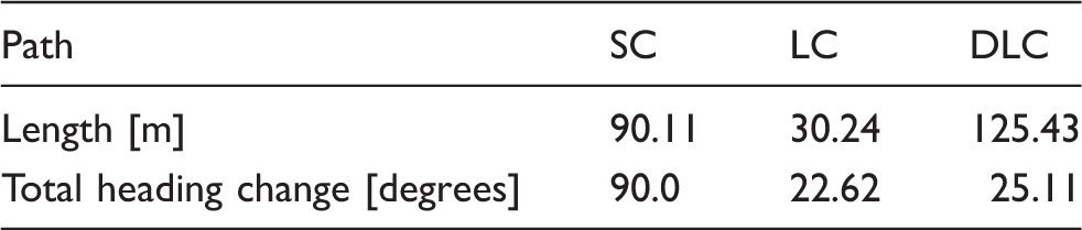
Path length and heading change for different experimental paths.

Path	SC	LC	DLC
Length [m]	90.11	30.24	125.43
Total heading change [degrees]	90.0	22.62	25.11

Table 2.

Vehicle parameters.

Parameter	m [Kg]	I_z [Kg/m²]	L [m]	a₁ [m]	a₂ [m]	C_ar [N/rad]	C_af [N/rad]	φ_max [deg]
	1000	1650	2.6	1.0	1.6	3000	3000	25

2.2. B-Spline reference paths

Reference paths are generated using B-spline curves as proposed in Elbanhawi et al. (2015a, 2014b). The resulting paths maintain continuous steering, velocity and acceleration trajectories. This resulted in reducing lateral forces acting on passengers and path tracking performance. This formulation is also guaranteed to be kinematically feasible. A p-th degree B-spline curve, c(u), is defined by n-number control points, P_i, m-number of knot vector, û, where m = n + p + 1 and i ∈ [1,n]. The knot vector consists of m non-decreasing real numbers, and u is a normalized curve length parameter. The curve c(u) is defined as the summation of each control points and its corresponding basis function as shown in equation (11). Where, P _i is the i-th control point and N_i,p(u) is the corresponding i-th B-spline basis function for c(u). The Cox-de Boor algorithm recursively evaluates the basis functions (De Boor, 1972), as given by equations (12) and (13). Initial calculation of the first set of basis functions is based on the knot vectors, û, as shown in equation (12). Higher degrees, from 2 to p, basis functions are evaluated using iterative substitution in (13). This recursive approach is often represented as a triangle structure of basis functions, where the base is first order, and recursion repeats until the p-th degree is calculated. The basis functions are substituted in equation (11) to generate the desired basis functions. Our earlier work guarantees path feasibility by modifying B-spline control points positioning and insertion (Elbanhawi et al., 2015a, 2015b).

c (u) = \sum_{i = 0}^{n} N_{i, p} (u) P_{i}

(11)

N_{i, 0} (u) = {1 u \in [{\hat{u}}_{i}, {\hat{u}}_{i + 1}) 0 else

(12)

N_{i, p} (u) = \frac{u - {\hat{u}}_{i}}{{\hat{u}}_{i + p} - {\hat{u}}_{i}} N_{i, p - 1} (u) + \frac{{\hat{u}}_{i + p + 1} - u}{{\hat{u}}_{i + p + 1} - {\hat{u}}_{i + 1}} N_{i + 1, p - 1} (u)

(13)

2.3. Pure pursuit path tracking

It is required to control a vehicle to track a predesigned path. The path is defined as a piecewise linear B-spline path, c(u), of J number of consecutive coordinates. In case of lateral control, the outputs of the controller are reference steering, φ, trajectories and the input is the reference (x_j y_j θ_i) positions, which were obtained from equation (11). The vehicle’s state, at step j, is calculated using equation (1b) (x′_j y′_j θ′_j), where j ∈ [1, J ]. The vehicle location is assumed to be fully observable and deterministic. Figure 3 is an illustration of the path tracking nomenclature used in this article.

Figure 3.

Pure pursuit path tracking schematic and nomenclature.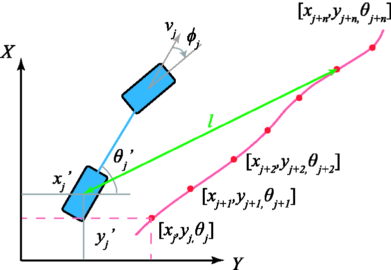

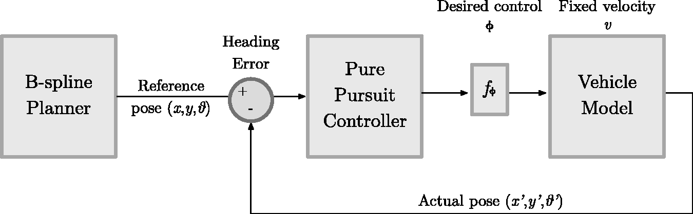
PP controller operates by steering based on the heading error, given in equation (14). The heading at any distance is determined by using curvilinear path parameters. The reference heading is measured at a distance from the vehicle referred to as the look-ahead distance. The look-ahead distance is a tuning parameter that is recommended to be a function on the velocity. Steering output was proportional to the heading error between the desired heading in the next step and current heading, as given by equation (15), where f_θ > 0. The traditional control scheme is illustrated in Figure 4.

θ_{j} = a \tan \frac{y_{j} - y_{j - 1}}{x_{j} - x_{j - 1}}

(14)

φ_{j} = f_{θ} (θ_{j + 1} - θ'_{j})

(15)

Figure 4.

Traditional Pure Pursuit control scheme.

2.4. Receding horizon pure pursuit control

The traditional PP control method does not account the vehicle dynamics when setting the desired steering command. The control signal is proportional to the heading error. Consequently, as the speed and the error grow, the steering command grows proportionally as well which leads to controller and vehicle instability (Snider, 2009). In this proposed approach there are three main changes to the PP controller. Initially, the PP heading error, equation (14), is used to calculate a desired yaw rate. The yaw rate set point is based on the steady state responses in equations (9) and (10). This accounts for vehicle dynamics and compensates the predicted steady state yaw rate. Finally, a RHC controller computes an optimal steering angle for the prediction, N_p, and control, N_c, horizons to achieve the desired steady state yaw rate set points. This approach is illustrated in Figure 5.

Figure 5.

Receding Horizon Control (RHC) Pure Pursuit (PP) control scheme.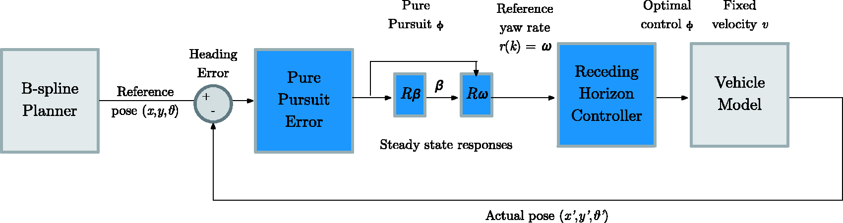

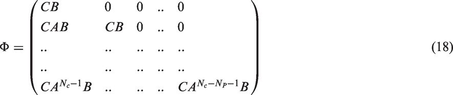
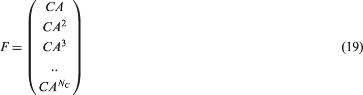
The optimal steering change in steering angle to achieve a desired yaw rate from current state is given in equation (17) as shown by Wang (2009). The current vehicle state x(k) and r(k) is the desired steady state yaw set point. The desired steady state yaw rate is calculated using the pure pursuit heading error and steady state responses at a fixed velocity (Jazar, 2008), as given in equation (17).

Δ φ * = (Φ T Φ + \bar{R}) - 1 Φ T ({\bar{R}}_{s} r (k) - Fx (k))

(16)

r (k) = R_{ω} \cos (R_{β} . φ_{pure pursuit}) . φ_{pure pursuit}

(17)

where, Φ and F are calculated, in equation (18) and (19), based on the lateral control model derived in equation (7) and (8).

Φ = (CB 00 . . 0 CAB CB 0 . . 0 . . . . . . . . . . . . . . . . . . . . CA N_{c} - 1 B . . . . . . CA N_{c} - N_{P} - 1 B)

(18)

F = (CA CA 2 CA 3 . . CA N_{C})

(19)

\bar{R_{s}} = J_{N_{c}, 1}

(20)

The controller can be tuned using a tuning parameter, r_w, equation (21). It balances the controller performance between minimizing tracking error (r_w tends to zero) and control effort (r_w tends to infinity).

\bar{R} = r_{ω} I_{N_{c} {XN}_{c}}

(21)

Therefore, the optimal control for any time instance is defined in equation (22).

φ_{k}^{*} = Δ φ * + φ_{k - 1}

(22)

3. Methodology

3.1. Setup

In this section, comparative analyses are conducted between PP controller and proposed RHC controller to highlight the performance of the proposed approach. Experiments are repeated for three different manoeuvres and six different speeds. Manoeuvre design, path generation, trajectory tracking and data analysis were conducted in Matlab environment.

3.2. Experiments

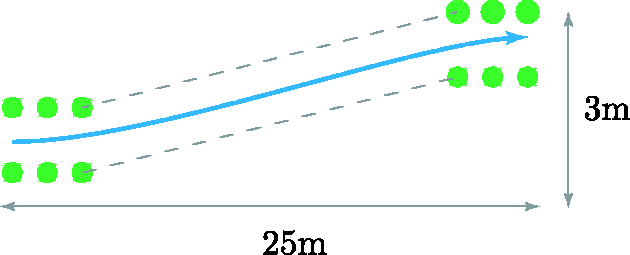
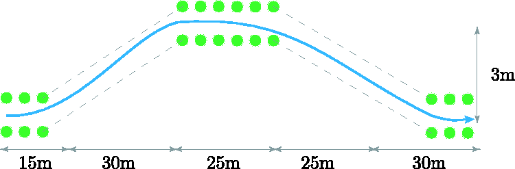
The paths selected for controller evaluation are commonly executed in street driving scenarios. Three different test cases were selected for controller evaluation. Step change (SC), shown in Figure 6, is a right hand turn; it is often used for path tracking control performance evaluation as proposed by Roth and Batavia (2002) and used in Cheein and Scaglia (2013). Lane change (LC), shown in Figure 7, is the most common on driving manoeuvre and is the cause of the majority of road accidents. LC was used as a test case for empirical study conducted in Snider (2009). Double Lane Change (DLC), shown in Figure 8, is a standard manoeuvre used to assess the lateral stability and manoeuvrability of vehicles (ISO 3888-1 (International Organisation for Standardisation), 1999).

Figure 6.

Step change (SC).

Figure 7.

Lane change (LC).

Figure 8.

Double lane change (DLC).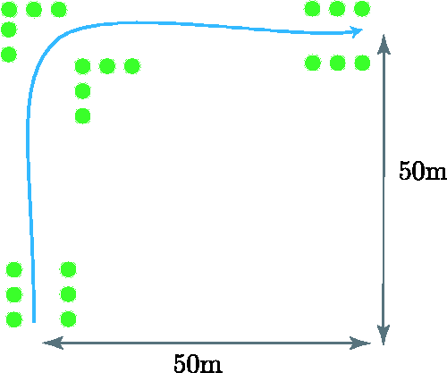

3.3. Reference paths

The tests paths were generated using the planning algorithm detailed earlier in section 2.2. The algorithm was used to generate three B-spline reference paths for SC, LC and DLC, as shown in Figure 9. Matlab data sets for the three paths are provided as supplementary files for this article (xyRefStep.dat, xyRefLC.dat, xyRefDI.dat). Additional path parameters are listed in Table 1.

Figure 9.

B-Spline paths for SC (top), LC (centre) and DLC (bottom).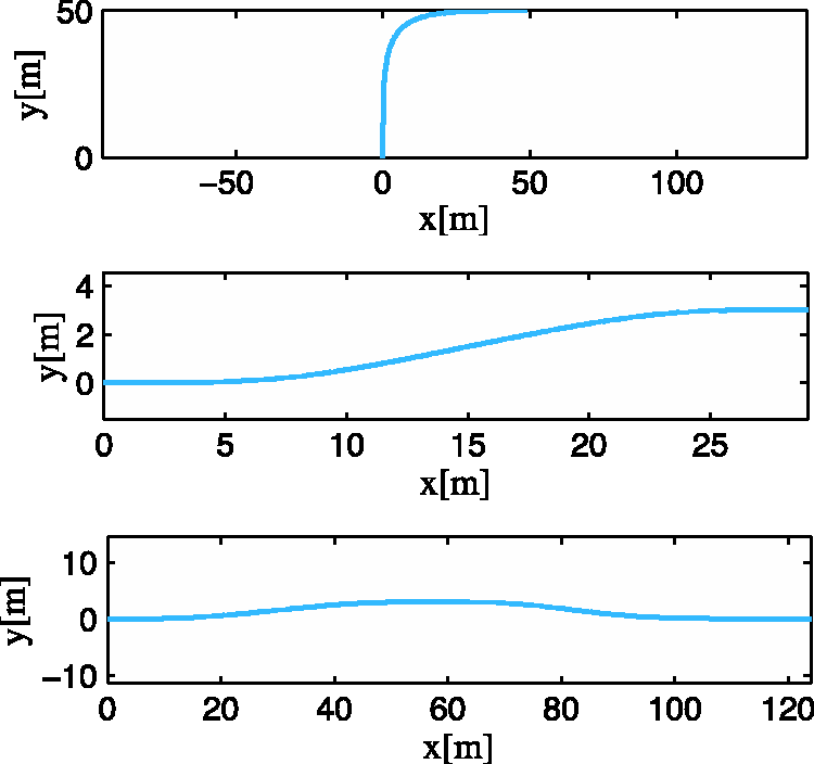

3.4. Vehicle parameters

The parameters for the vehicle considered in this experiment are detailed in Table 2. These are used for the vehicle model equation (7) and (8) and the steady state responses in equation (9) and (10).

Longitudinal speed was kept constant for each experiment as mentioned earlier. The speeds were varied incrementally from 1 m/s (3.6 Km/h) up to 20 m/s (72 Km/h) for different experiments.

4. Results

This section details the results for a total of 36 independent different experiments. The experiments are repeated with systematic changes in the path topology and speeds to validate the performance for both controllers.

Two controllers: traditional PP and proposed RHC-PP.

Three environments: SC, LC and DLC.

Six test speeds: 1, 2.5, 5, 10, 15 and 20 [m/s].

The aim of these experiments was to evaluate,

The vehicle stability by measuring the side-slip angle (Tondel and Johansen, 2005).

Controller performance by showing the control signals, measuring the control effort and tracking error (Roth and Batavia, 2002).

The RHC control horizon and prediction horizons were set to 15 and 50 steps. Whilst, changes in the horizon did not alter the control performance we intend to conduct a parametric study as part of our future research.

4.1. Side slip

This results for the steady state side slip angles for different controllers and speeds are given in this section.

4.1.1. Step change (SC)

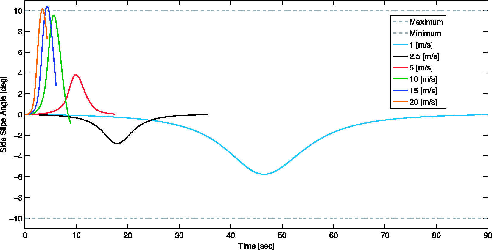
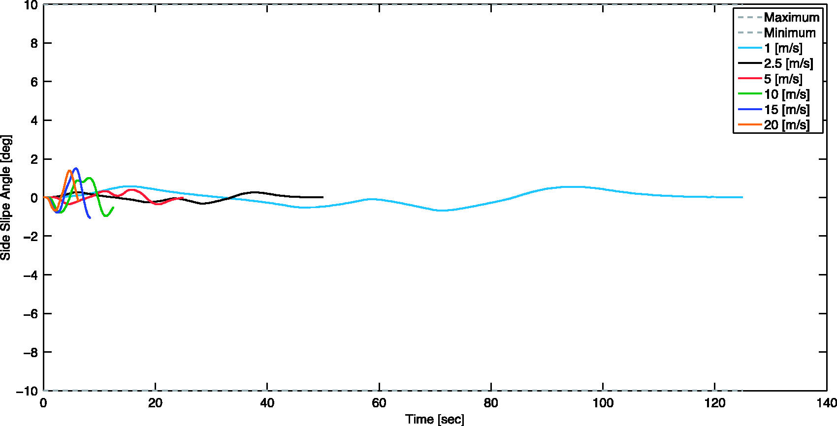
The side slip for SC case using traditional PP and proposed RHC-PP at different speeds is shown in Figures 10 and 11 respectively.

Figure 10.

Side slip angles for SC experiment using traditional pure pursuit.

Figure 11.

Side slip angles for SC experiment using proposed RHC pure pursuit.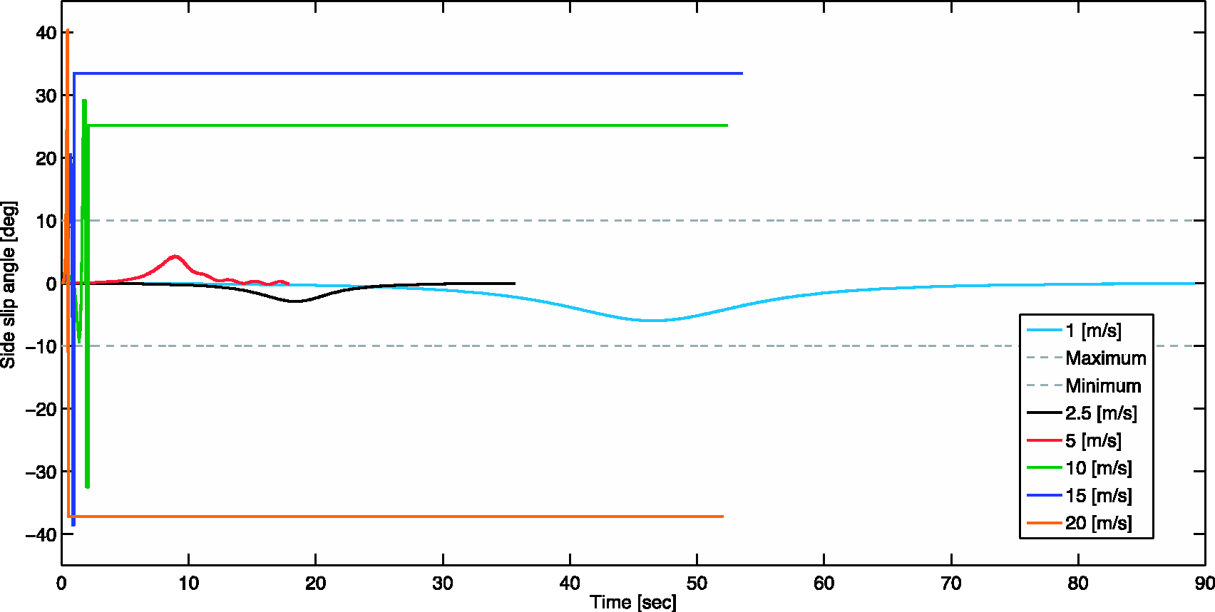

4.1.2. Lane change (LC)

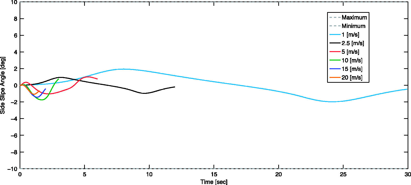
The side slip for LC case using traditional PP and proposed RHC-PP at different speeds is shown in Figures 12 and 13 respectively.

Figure 12.

Side slip angles for LC experiment using traditional pure pursuit.

Figure 13.

Side slip angles for LC experiment using proposed RHC pure pursuit.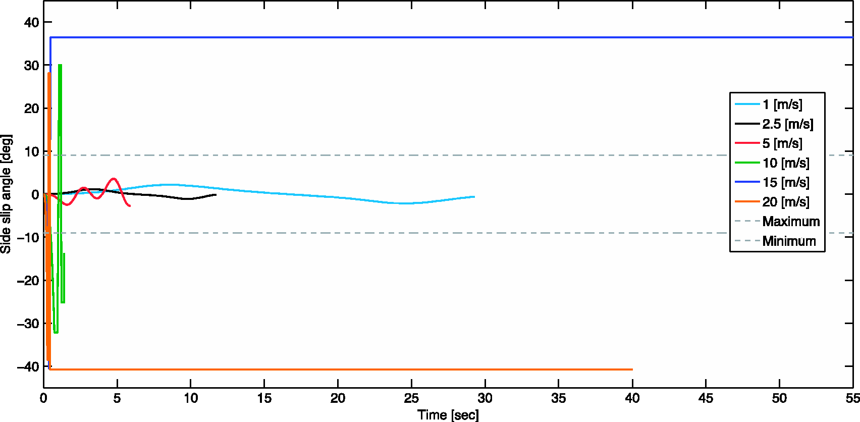

4.1.3. Double lane change (DLC)

The side slip for DLC case using traditional PP and proposed RHC-PP at different speeds is shown in Figures 14 and 15 respectively.

Figure 14.

Side slip angles for DLC experiment using traditional pure pursuit.

Figure 15.

Side slip angles for DLC experiment using proposed RHC pure pursuit.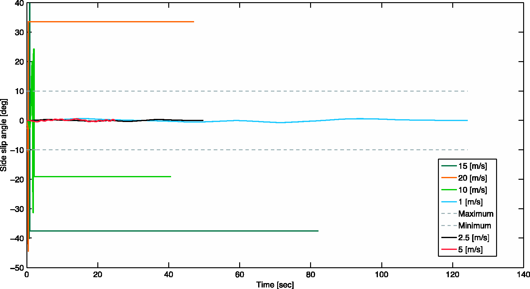

4.2. Control signals

The control signals for both controllers are shown in this section to evaluate the controller performance as the speed increases for the different test cases. For PP controller the steering angle and velocity for each path is shown. For the proposed RHC controller, the reference and output yaw rate are shown in addition to the steering angle and velocity.

4.2.1. Step change (SC)

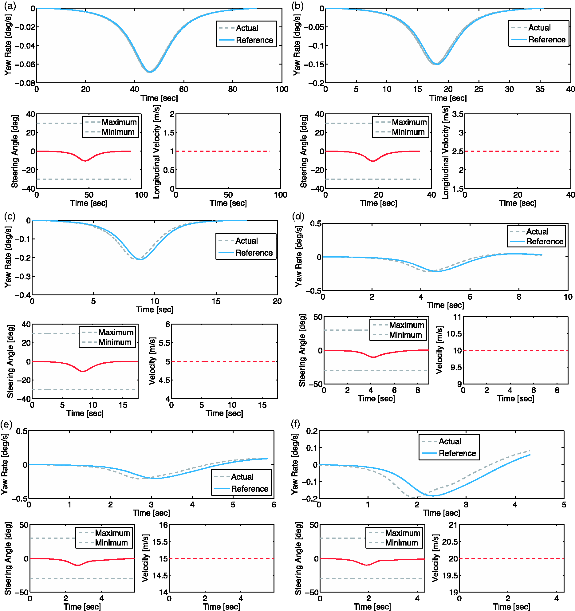
Control signal for SC using traditional and proposed PP controllers are shown in Figures 16 and 17 respectively.

Figure 16.

Control signals for SC at (a) 1 m/s (b) 2.5 m/s (c) 5 m/s.

Figure 17.

Proposed RHC control signals for SC at (a)1 m/s (b)2.5 m/s (c)5 m/s (d)10 m/s (e)15 m/s (f)20 m/s.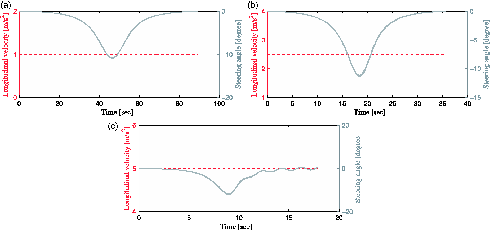

4.2.2. Lane change (LC)

Control signal for LC using traditional and proposed PP controllers are shown in Figures 18 and 19 respectively.

Figure 18.

Control signals for LC at (a) 1 m/s (b) 2.5 m/s (c) 5 m/s.

Figure 19.

Proposed RHC control signals for LC at (a)1 m/s (b)2.5 m/s (c)5 m/s (d)10 m/s (e)15 m/s (f)20 m/s.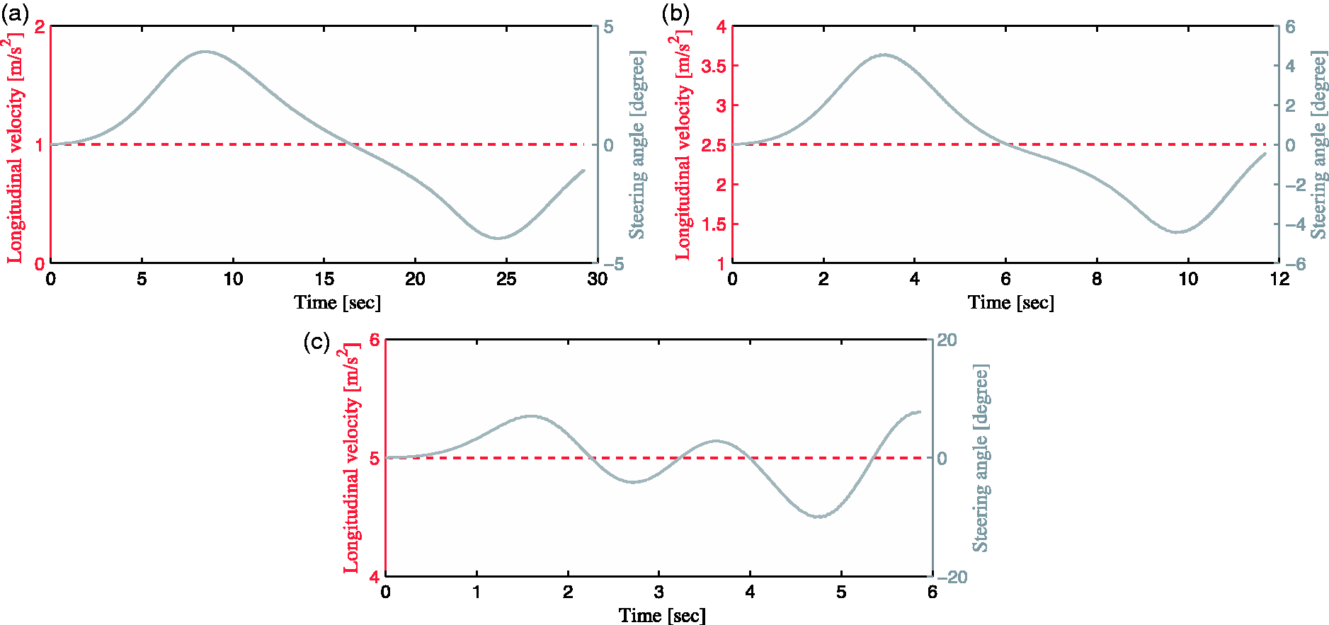

4.2.3. Double lane change (DLC)

Control signal for DLC using traditional and proposed PP controllers are shown in Figures 20 and 21 respectively.

Figure 20.

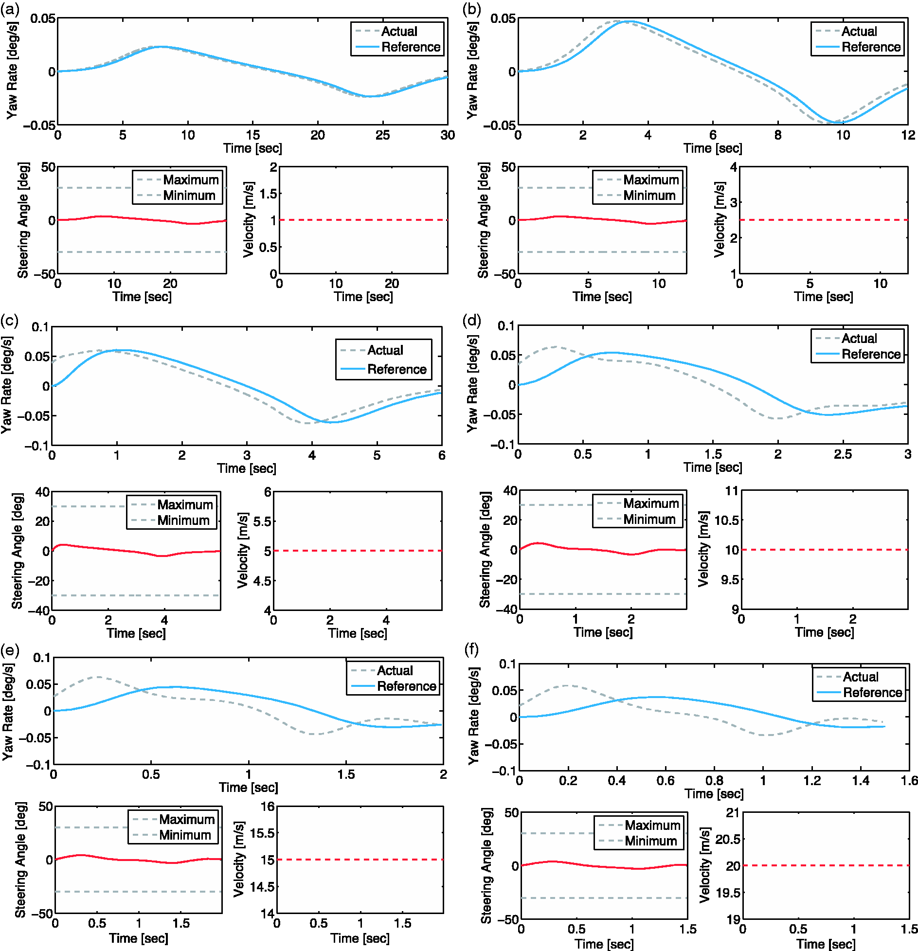
PP control signals for DLC at (a) 1 m/s (b) 2.5 m/s (c) 5 m/s.

Figure 21.

Proposed RHC control signals for DLC at (a)1 m/s (b)2.5 m/s (c)5 m/s (d)10 m/s (e)15 m/s (f)20 m/s.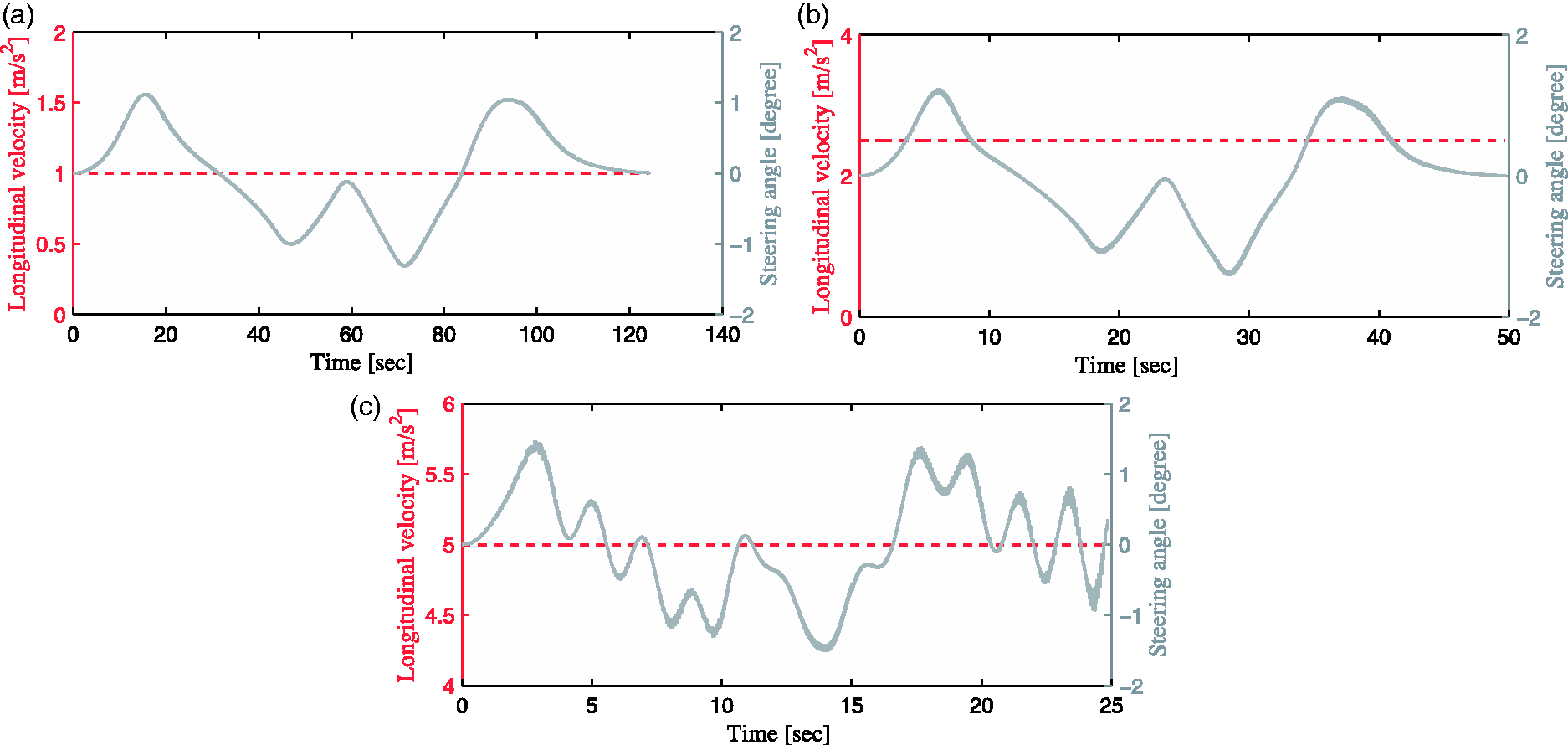

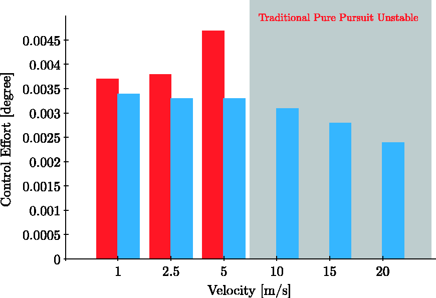
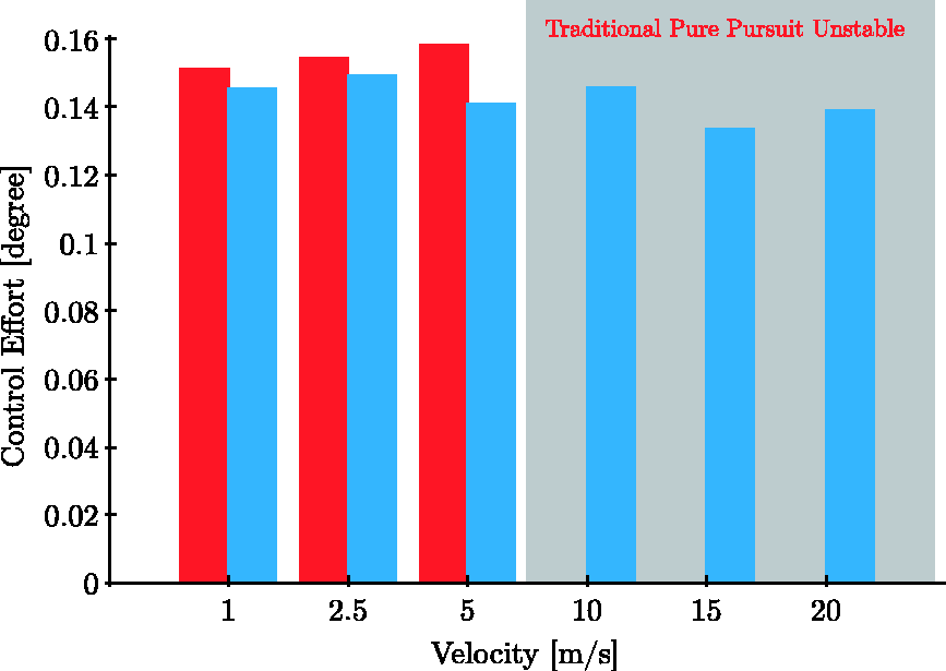
4.3. Control effort

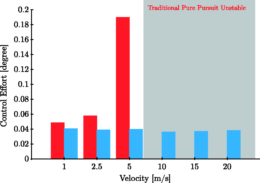
The control efforts for both controllers are shown in this section to evaluate the controller performance as the speed increases for the different test cases. For lateral control with fixed velocity the control effort is calculated using equation (23). The total control effort for both controllers in SC, LC and DLC cases are given in Figures 22–24 respectively. The results for traditional PP are not shown for speeds above 5 m/s as the controller became unstable and could not execute the paths.

E_{φ} = \sum_{i = 0}^{n} \frac{1}{2} φ 2

(23)

4.4. Tracking errors

The evaluation of the controller performance as the speed increases for the different test cases is continued using tracking errors. Cross track error and heading errors were evaluated for both controllers. The results for traditional PP are not shown for speeds above 5 m/s as the controller became unstable and could not execute the paths.

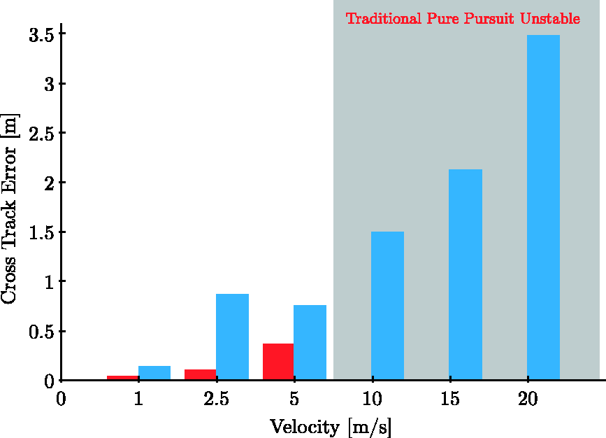
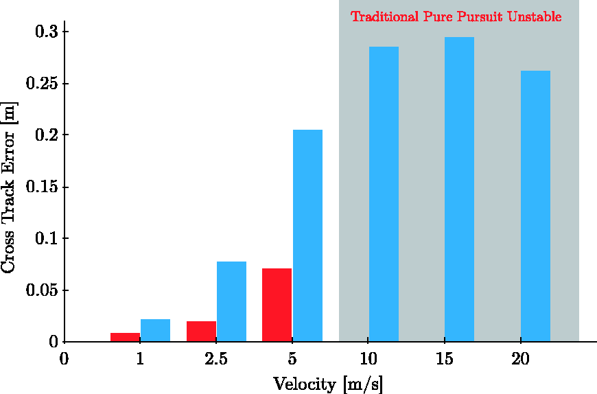
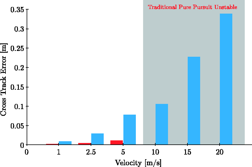
4.4.1. Cross track error

The total cross track error is calculated using equation (24). The total cross track error for both controllers in SC, LC and DLC cases are given in Figures 25–27 respectively.

E_{x, y} = \sum_{i = 0}^{n} \sqrt{(x_{i} - x'_{i}) 2 + (y_{i} - y'_{i}) 2}

(24)

Figure 22.

Control effort for SC using traditional (red) and RHC (blue) pure pursuit.

Figure 23.

Control effort for LC using traditional (red) and RHC (blue) pure pursuit.

Figure 24.

Control effort for DLC using traditional (red) and RHC (blue) pure pursuit.

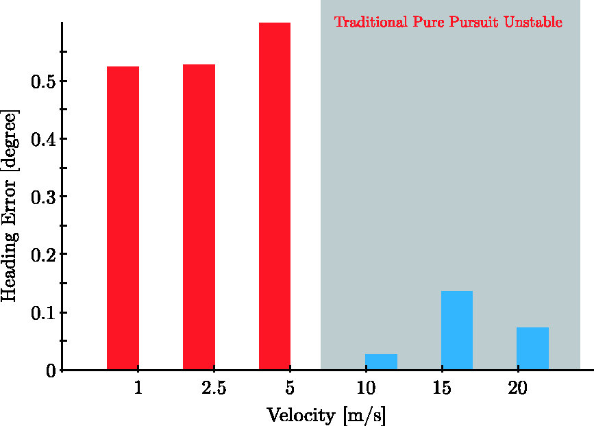
4.4.2. Heading error

The total heading error is calculated using equation (25). The total cross track error for both controllers in SC, LC and DLC cases are given in Figures 28–30 respectively.

E_{φ} = \sum_{i = 0}^{n} \frac{1}{2} θ_{i}^{2}

(25)

Figure 25.

Cross track error for SC using traditional (red) and RHC (blue) pure pursuit.

Figure 26.

Cross track error for LC using traditional (red) and RHC (blue) pure pursuit.

Figure 27.

Cross track error for DLC using traditional (red) and RHC (blue) pure pursuit.

5. Track experiments

In this section, the proposed RHC controller performance is demonstrated on a closed circuit track (CCT). The experiment setup is replicated for the standard manoeuvres in section 4. A B-spline path is generated for reference path. The path is subdivided into smaller successive segments and the controller generates.

5.1. Closed circuit track

The close circuit path is plotted with the corresponding B-spline reference path in Figure 31. The path is 1643.1 m long. A constant look-ahead distance of 2.6 m is maintained for speeds below 10 m/s and 5 m for higher speeds. The tuning parameter r_w was set to 1000.

Figure 31.

Reference closed circuit track (grey) and corresponding B-spline path.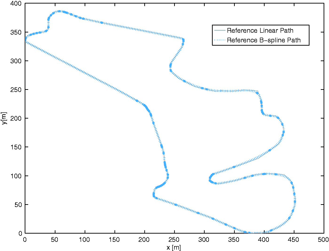

5.2. Results

5.2.1. Control signals

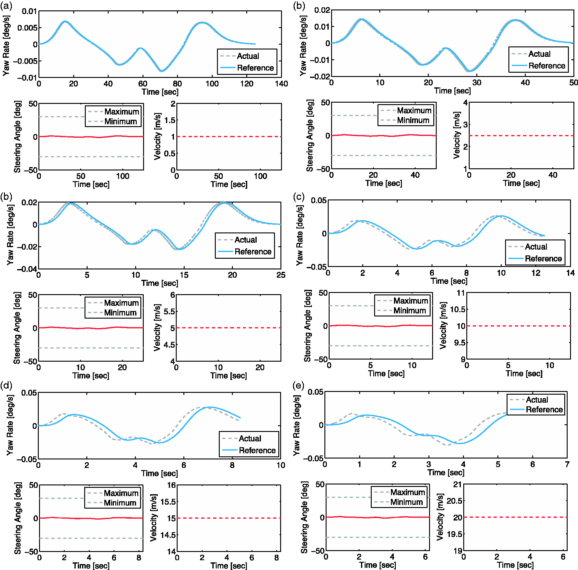
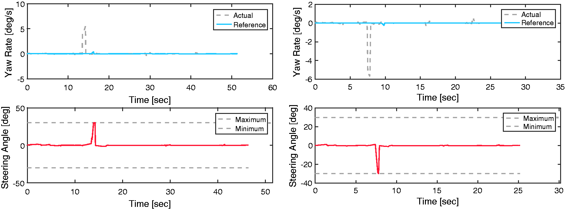
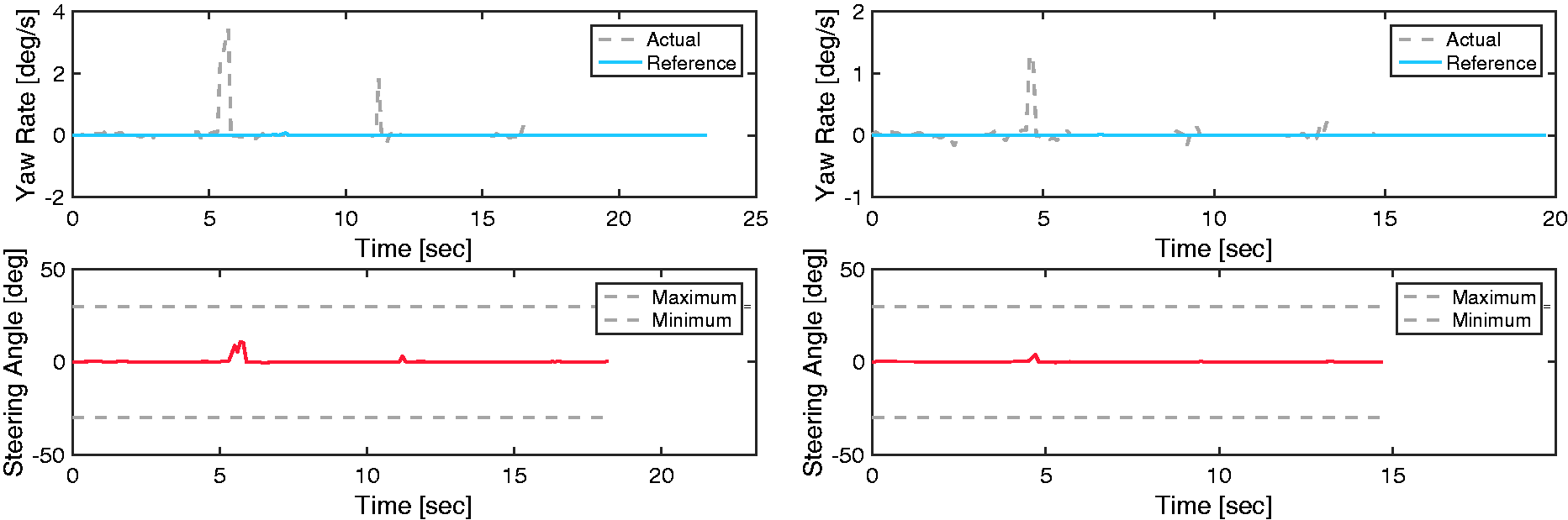
The control signals for RHC controller are shown in this section to evaluate the controller performance as the speed increases for the test cases. The reference and output yaw rate are shown in addition to the steering angle and velocity in Figures 32–34.

Figure 32.

Proposed RHC control signals for CCT at v = (left) 1 m/s (right) 2.5 m/s.

Figure 33.

Proposed RHC control signals for CCT at v = (left) 5 m/s (right) 10 m/s.

Figure 34.

Proposed RHC control signals for CCT at v = (left) 15 m/s (right) 20 m/s.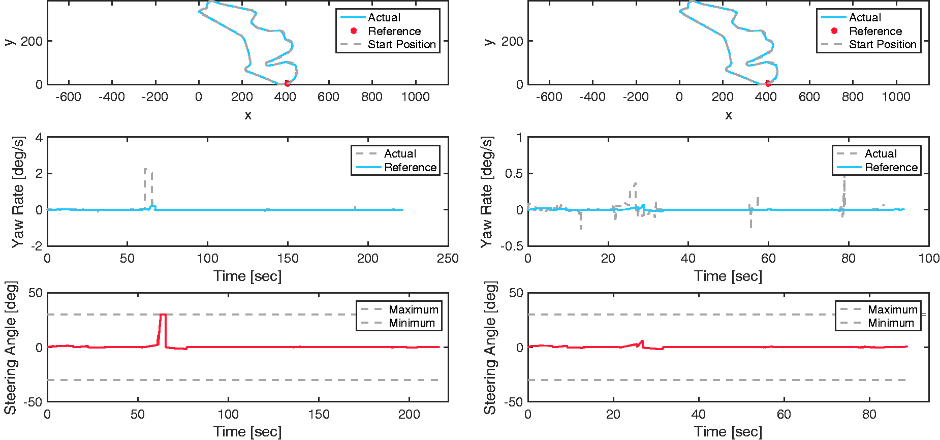

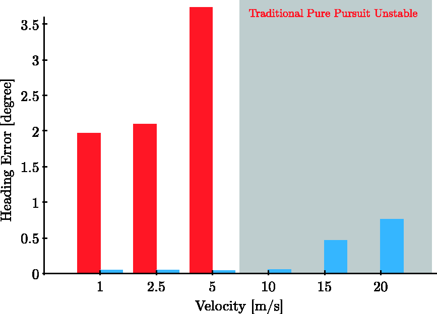
5.2.2. Tracking performance

The tracking performance for the proposed CCT experiments is presented. The control signals presented in the previous section were conducted for a tuning parameter value r_w = 1000. The tracking results are compared when setting the tuning parameter to 10. As mentioned earlier, the tuning parameter balances the performance between minimizing the control error and the control effort. The cross track error, heading error and control effort results are given in Figures 35–37. A large tuning parameter value reduced the controller effort and produce control signals that are realistic for the actuator. The low tuning parameter reduced the heading and cross track errors. It is clear that both parameter values are extreme but they showcase the ability of the controller to track the closed circuit path. It is difficult to conclude which parameter value has improved the tracking performance. This decision is based on the designer choice and the intended use of the autonomous vehicle.

Figure 35.

CCT cross track error.

Figure 36.

CCT heading error.

Figure 37.

CCT controller effort.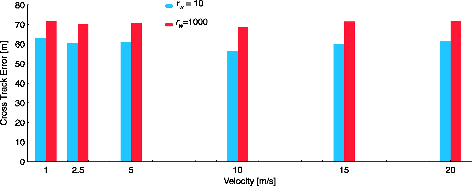

5.2.3. Side slip

Side slip angle results for CCT using RHC PP controller for the different velocities are illustrated in Figure 38.

6. Discussion

6.1. Controller performance

The tracking error and control effort are used to evaluate the performance of tracking controllers (Roth and Batavia, 2002; Cheein and Scaglia, 2013). The controller is designed to balance both error and effort values as they are conflicting characteristics.

First, we consider the controller effort. The steering control signals, in section 4.2, can be used as a visual representation of the effort and the total control effort are given in section 4.3. In case of the traditional PP, as the speed increases, the steering control exhibited oscillations and the controller became unstable at speeds higher than 5 m/s. This is can be noted by observing the results in Figures 16, 18 and 20. The traditional PP control signal is proportional to the heading error. The increasing effort relative to vehicle speed was consistent across all experiments as shown in Figures 22–24, regardless of the heading errors, which did not increase significantly with speed for the conducted experiments Figures 28–30. It is clear that the traditional controller deteriorated as the speed increased and eventually became unstable. On the other hand, the controller effort for the proposed method was consistent irrespective of the increasing speed and tracking errors. This can be shown by observing the control signals in Figures 17, 19, and 21. The aggregate control effort values are shown in Figures 22–24.

Figure 28.

Heading error for SC using traditional (red) and RHC (blue) pure pursuit.

Figure 29.

Heading error for LC using traditional (red) and RHC (blue) pure pursuit.

Figure 30.

Heading error for DLC using traditional (red) and RHC (blue) pure pursuit.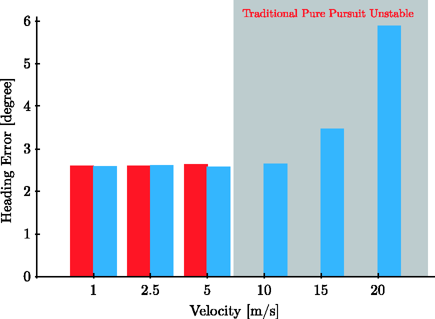

For all paths, the RHC control effort remained constant and was less than that of the traditional PP controller. This is the result of the proposed modification in the PP control scheme as shown in Figure 5. The proposed controller does not rely on the heading error as input to the controller and uses the steady state yaw rate as a reference. Additionally, the proposed controller was tuned to balance the control effort and error by setting the tuning parameter to a conservative value, r_w = 10, in equations (21) then (16). The reduction in control effort is a significant parameter for autonomous vehicles. It was related to improving passenger comfort, reducing mechanical wear, improving vehicle efficiency and stability.

The tracking, cross-track and heading, errors were noted to increase with speed. For any class of PP controllers, this behaviour is expected since they rely on the heading error for lateral guidance. The aggregate tracking errors for both controllers are compared in Figures 25–27. Nonetheless, when considering the heading error it is clear that our proposed controller improves the lateral guidance performance. The total heading error results for both controllers are evaluated in Figures 28–30. Despite not relying on the heading error as an input to the controller, the RHC reduced the heading error in comparison to PP. It is worth noting that both heading and tracking error are relatively low when considering the path length and heading change for the reference paths Table 1.

For the closed circuit experiment, the proposed controller was capable of tracking the path successfully. The tuning parameter has a clear effect on the tracking performance. A low value reduced tracking errors but increased control effort. The parameter decision is based on the desired application of the vehicle. As is the case with RHC, a study of the parameters effect prior to implementing the controller is needed for any application.

6.2. Vehicle stability

The vehicle lateral stability was evaluated based on the side slip angle and vehicle velocity, as given in equation (26) (Tondel and Johansen, 2005; Attia et al., 2014).

β_{\max} = 10 - 7 \frac{v 2}{40}

(26)

For all experiments and speed the RHC proposed controller maintained the vehicle below the slide slip limitations as given in Figures 11, 13 and 15. However, the error based traditional PP failed to maintain the vehicle stable at speed higher than 5 m/s in all experiments. This is a result of the proportionality between the steering and the error for PP, as the speed increased, the error also grew and the change in steering angle, consequently, increased. However in the case of RHC controller increasing the error did not directly translate to an increase in the control signal as discussed in the controller performance. This is apparent for all cases when comparing the tracking errors, which are growing with velocity as shown in Figures 25–27. For the same cases, the side slip angle is maintained within the same range at increasing tracking speeds as mentioned earlier. Significant changes in the steering angles at high speeds led to large increases in the slip angle, as governed by equation (9). This is reflected by the ability of the proposed controller to maintain small slip angles at higher speeds as the control signal becomes relatively independent of the vehicle speed.

6.3. Controller limitations and further recommendations

The proposed strategy has improved the PP control performance and resulting vehicle stability, as discussed earlier. However, there are some limitations that are the subjects of future studies. The steering angle (control signal) saturation limits are implemented as soft constraints as described in (Cheein and Scaglia, 2013). The control signal limitations could as a linear inequality and the control signal be modelled as a quadratic optimisation problem (Hildreth, 1957). The lateral guidance model derived for this controller was based on the yaw rate and slip angles and does not account for the cross track error. Path error-based lateral control models for front wheel steering have been developed (Soudbakhsh and Eskandarian, 2012). These models may contribute to reducing the cross-track error but they have been shown to be less robust to external disturbances and path continuity (Snider, 2009). Motivated by the presented numerical results, we intend to evaluate the controller for field testing and stochastic actuation. However, field testing, for high speed navigation, is an engineering challenge for experimental autonomous platform. An early demonstration of the performance of the algorithm for representative driving environments is given in section 5 for the closed circuit track. The tracking results for CCT with different tuning parameters highlight the effect of the parameters on the planner performance. Parametric analyses of the influence of prediction horizon, control horizon and look-ahead distance will be conducted to optimise the parameter selection using Monte Carlo experiments.

Footnotes

Acknowledgments

The authors would like to thank Mr Hormoz Marzbani for insightful discussions. The anonymous reviewers provided the closed circuit track used in section 5.

Declaration of Conflicting Interests

The author(s) declared no potential conflicts of interest with respect to the research, authorship, and/or publication of this article.

Funding

The author(s) disclosed receipt of the following financial support for the research, authorship, and/or publication of this article: Mr Elbanhawi acknowledges the financial support of the Australian Postgraduate Award (APA) and the Research Training Scheme (RTS).

Appendix 100KPH

References

Aripin

Md Sam

Danapalasingam

et al. (2014) A Review of Active Yaw Control System for Vehicle Handling and Stability Enhancement. International Journal of Vehicular Technology 2014: 1–15.

Attia

Orjuela

Basset

(2014) Combined longitudinal and lateral control for automated vehicle guidance. Vehicle System Dynamics 52: 261–279.

Beal

Gerdes

(2013) Model Predictive Control for Vehicle Stabilization at the Limits of Handling. Control Systems Technology, IEEE Transactions on 21: 1258–1269.

Bengler

Dietmayer

Farber

et al. (2014) Three Decades of Driver Assistance Systems: Review and Future Perspectives. Intelligent Transportation Systems Magazine, IEEE 6: 6–22.

Bureau of Infrastructure Transport and Regional Economics (BITRE) (2014) Road Deaths Australia. 2013 Statistical Summary BITRE, Canberra ACT.

Bureau of Transportation Statistics (2013) Household Travel Survery Report: Sydney 2012/13. In: Transport for NSW (ed). Sydney, NSW.

Bureau of Transportation Statistics (2014) National Transportation Statistics, U.S. Department of Transportation.

Campion

Bastin

Dandrea-Novel

(1996) Structural properties and classification of kinematic and dynamic models of wheeled mobile robots. Robotics and Automation, IEEE Transactions on 12: 47–62.

Cheein

Scaglia

(2013) Trajectory Tracking Controller Design for Unmanned Vehicles: A New Methodology. Journal of Field Robotics 31: 861–887.

10.

Corke

(2011) Robotics, Vision and Control: Fundamental Algorithms in MATLAB, Berlin, Germany: Springer.

11.

Craig

(1992) Implementation of the Pure Pursuit Path Tracking Algorithm, Pittsburgh, Pennsylvania, USA: Carnegie Mellon University.

12.

De Boor

(1972) On calculating with B-splines. Journal of Approximation Theory 6: 50–62.

13.

Dolgov

Thrun

(2009) Autonomous driving in semi-structured environments: Mapping and planning. Robotics and Automation, 2009. ICRA ‘09. IEEE International Conference on. 3407–3414.

14.

Elbanhawi

Simic

(2014) Sampling-Based Robot Motion Planning: A Review. Access, IEEE 2: 56–77.

15.

Elbanhawi

Simic

Jazar

(2015a) Continuous Path Smoothing for Car-Like Robots Using B-Spline Curves. Journal of Intelligent & Robotic Systems. 80: 23–56.

16.

Elbanhawi

Simic

Jazar

(2015b) Improved Manoeuvring of Autonomous Passenger Vehicles: Simulations and Field Results. Journal of Vibration and Control (In press). doi: 10.1177/1077546315605666, Published online, pager 1=30.

17.

Fagnant

Kockelman

(2014) The travel and environmental implications of shared autonomous vehicles, using agent-based model scenarios. Transportation Research Part C: Emerging Technologies 40: 1–13.

18.

Fairfield N and Urmson C (2011) Traffic light mapping and detection. Robotics and Automation (ICRA), 2011 IEEE International Conference on, Shanghai, 2011, pp. 5421–5426. doi: 10.1109/ICRA.2011.5980164.

19.

Falcone

Borrelli

Asgari

et al. (2007) Predictive Active Steering Control for Autonomous Vehicle Systems. Control Systems Technology, IEEE Transactions on 15: 566–580.

20.

Geiger

Lenz

Stiller

et al. (2013) Vision meets robotics: The KITTI dataset. The International Journal of Robotics Research 32: 1231–1237.

21.

(2002) Neural predictive control for a car-like mobile robot. Robotics and Autonomous Systems 39: 73–86.

22.

(2006) Receding horizon tracking control of wheeled mobile robots. Control Systems Technology, IEEE Transactions on 14: 743–749.

23.

McCarley

Kramer

(2014) Lane Keeping Under Cognitive Load: Performance Changes and Mechanisms. Human Factors: The Journal of the Human Factors and Ergonomics Society 56: 414–426.

24.

Hildreth

(1957) A quadratic programming procedure. Naval Research Logistics Quarterly 4: 79–85.

25.

ISO 3888-1 (International Organisation for Standardisation) (1999) Passenger cars — Test track for a severe lane-change manoeuvre — Part 1: Double Lane Change.

26.

Jazar

(2008) Vehicle Dynamics: Theory and Application, Springer Science+Business Media, LLC, 233 Spring Street, New York, NY 10013, USA: Springer.

27.

Kuffner

LaValle

(2000) RRT-connect: An efficient approach to single-query path planning. Robotics and Automation, 2000. Proceedings. ICRA ‘00. IEEE International Conference on 1002: 995–1001.

28.

Kusano

Gabler

(2012) Safety Benefits of Forward Collision Warning, Brake Assist, and Autonomous Braking Systems in Rear-End Collisions. Intelligent Transportation Systems, IEEE Transactions on 13: 1546–1555.

29.

Laurgeau

(2012) Intelligent Vehicle Potential and Benefits. In: Eskandarian

(ed.) Handbook of Intelligent Vehicles. London: Springer, pp. 1537–1551.

30.

Lee

(2008) Fifty Years of Driving Safety Research. Human Factors: The Journal of the Human Factors and Ergonomics Society 50: 521–528.

31.

Lenain

Thuilot

Cariou

et al. (2009) Mixed kinematic and dynamic sideslip angle observer for accurate control of fast off-road mobile robots. Journal of Field Robotics.

32.

Likhachev

Ferguson

Gordon

et al. (2008) Anytime search in dynamic graphs. Artificial Intelligence 172: 1613–1643.

33.

Xue

Kawabata

et al. (2015) Efficient Sampling-Based Motion Planning for On-Road Autonomous Driving. Intelligent Transportation Systems, IEEE Transactions on. 1–16..

34.

Marzbani

Ahmad Salahuddin

Simic

et al. (2014) Steady-state dynamic steering. Frontiers in Artificial Intelligence and Applications. 493–504.

35.

Marzbani

Jazar

Fard

(2015) Steady-State Vehicle Dynamics. In: Dai

Jazar

(eds) Nonlinear Approaches in Engineering Applications. Springer Science+Business Media, LLC, 233 Spring Street, New York, NY 10013, USA: Springer International Publishing, pp. 3–30.

36.

Mayne

(2014) Model predictive control: Recent developments and future promise. Automatica 50: 2967–2986.

37.

Milanes

Villagra

Perez

et al. (2012) Low-Speed Longitudinal Controllers for Mass-Produced Cars: A Comparative Study. Industrial Electronics, IEEE Transactions on 59: 620–628.

38.

Morris

Humphrey

Pickering

et al.

The Department for Transport (2013) National Travel Survey 2013. London, UK: NatCen Social Research.

39.

NHTSA (National Highway Traffic Safety Administration) (2013) Preliminary Statement of Policy Concerning Automated. Vehicles. 1–14.

40.

Pacejka

(2006) Tyre and Vehicle Dynamics, Oxford, UK: Butterworth-Heinemann.

41.

Pandey

McBride

Eustice

(2011) Ford Campus vision and lidar data set. The International Journal of Robotics Research 30: 1543–1552.

42.

Payre

Cestac

Delhomme

(2014) Intention to use a fully automated car: Attitudes and a priori acceptability. Transportation Research Part F: Traffic Psychology and Behaviour 27: 252–263.

43.

Petrov

Nashashibi

(2013) Adaptive steering control for autonomous lane change maneuver. Intelligent Vehicles Symposium (IV), 2013 IEEE. 835–840.

44.

Preston

(2014) What does the public think about driverless cars?. Available at: http://www.virgin.com/disruptors/infographic-what-does-the-public-think-about-driverless-cars (accessed 18 October 2014).

45.

Rajamani

(2012) Lateral Vehicle Dynamics. Vehicle Dynamics and Control, USA: Springer, pp. 15–46.

46.

Roth

Batavia

(2002) Evaluating Path Tracker Performance for Outdoor Mobile Robots. Automation Technology for Off-Road Equipment, Chicago, Illinois, USA: American Society of Agricultural and Biological Engineers, pp. 399–397.

47.

Saleh

Chevrel

Claveau

et al. (2013) Shared Steering Control Between a Driver and an Automation: Stability in the Presence of Driver Behavior Uncertainty. Intelligent Transportation Systems, IEEE Transactions on 14: 974–983.

48.

Santos

McGuckin

Nakamoto

et al. (2011) Summary of Travel Trends: 2009 National Household Travel (NTS) Survery, New Jersey, SE, Washington, DC, US: Department of Transporation.

49.

Schoettle

Sivak

(2014a) Public Opinion about Self-Driving Vehicles in China, India, Japan, the US, the UK and Australia, Michigan: The University of Michigan Sustainable Worldwide Transportation.

50.

Schoettle

Sivak

(2014b) A Survey of Public Opinion about Autonomous and Self-Driving Vehicles in the US, the UK and Australia, Michigan: The University of Michigan Sustainable Worldwide Transportation.

51.

Serrano

Scaglia

GJE

Cheein

et al. (2014) Trajectory-tracking controller design with constraints in the control signals: a case study in mobile robots. Robotica. FirstView: 1–18.

52.

Snider

(2009) Automatic steering methods for autonomous automobile path tracking. Robotics Institute, Pittsburgh, PA, Tech. Rep. CMU-RITR-09-08.

53.

Soudbakhsh

Eskandarian

(2012) Vehicle Lateral and Steering Control. In: Eskandarian

(ed.) Handbook of Intelligent Vehicles. Springer London, pp. 209–232.

54.

Talvala

KLR

Kritayakirana

Gerdes

(2011) Pushing the limits: From lanekeeping to autonomous racing. Annual Reviews in Control 35: 137–148.

55.

Thorpe

Herbert

Kanade

et al. (1991a) Toward autonomous driving: the CMU Navlab. I. Perception. IEEE Expert 6: 31–42.

56.

Thorpe

Herbert

Kanade

et al. (1991b) Toward autonomous driving: the CMU Navlab. II. Architecture and systems. IEEE Expert 6: 44–52.

57.

Thrun

Montemerlo

Dahlkamp

et al. (2007) Stanley: The Robot That Won the DARPA Grand Challenge. In: Buehler

Iagnemma

Singh

(eds) The 2005 DARPA Grand Challenge. Berlin: Springer Heidelberg, pp. 1–43.

58.

Tondel

Johansen

(2005) Control allocation for yaw stabilization in automotive vehicles using multiparametric nonlinear programming. Proceedings of the 2005, American Control Conference. 453–458. . doi: 10.1109/ACC.2005.1469977.

59.

van Winsum

(1996) Speed choice and steering behavior in curve driving. Human Factors 38: 434.

60.

van Winsum

de Waard

Brookhuis

(1999) Lane change manoeuvres and safety margins. Transportation Research Part F: Traffic Psychology and Behaviour 2: 139–149.

61.

van Zanten

(1999) ESP Electronic Stability Program.. Robert Bosch GmbH.

62.

van Zanten

(2000) Bosch ESP systems: 5 years of experience. SAE Technical Papers.

63.

Waldrop

(2015) Autonomous vehicles: No drivers required. Nature 518: 20.

64.

Wang

(2009) Model Predictive Control System Design and Implementation Using MATLAB, Springer-Verlag, London, UK: Springer Publishing Company, Incorporated.

65.

Wang

Teoh

Shen

(2004) Lane detection and tracking using B-Snake. Image and Vision Computing 22: 269–280.

66.

Zheng

(2014) Recent developments and research needs in modeling lane changing. Transportation Research Part B: Methodological 60: 16–32.