Oblique Impact of Multi-Flexible-Link Systems

Abstract

The main goal of this paper is to present an automatic approach for the dynamic modeling of the oblique impact of a multi-flexible-link robotic manipulator. The behavior of a multi-flexible-link system confined inside a closed environment with curved walls can be completely expressed by two distinct mathematical models. A set of differential equations is employed to model the system when it has no contact with the curved walls (Flight phase); and a set of algebraic equations is used whenever it collides with the confining surfaces (Impact phase). In this article, in addition to the Assumed Mode Method (AMM), the Euler-Bernoulli Beam Theory (EBBT), and the Newton’s kinematic impact law, the Gibbs-Appell (G-A) formulation has been employed to derive the governing equations in both phases. Also, instead of using 3 × 3 rotational matrices, which involves lengthy kinematic and dynamic formulations for deriving the governing equations, 4 × 4 transformation matrices have been used. Moreover, for the systematic modeling of flexible multiple links through the space, two virtual links have been added to the n real links of a manipulator. Finally, two case studies have been simulated to demonstrate the validity of the proposed approach.

Keywords

4 × 4 transformation matrix oblique impact flexible manipulator symbolic derivation Gibbs-Appell formulation

1. Introduction

When a multibody system is subjected to impact forces that may originate from external impulses or impulsive constraints, the velocity of every component of that system can change abruptly. The dynamic modeling of a flexible robotic manipulator confined inside a closed environment has many engineering applications. For example, in the mathematical modeling of humanoid robotic systems that walk on the ground and may collide with side barriers, it is necessary to know what happens during the pre-impact, impact and post-impact time intervals. In fact, the viscoelastic properties of the muscles that cover human bones justify the use of flexible links in the modeling of bipedal robotic systems.

The impact phenomena related to multibody systems have already been well formulated. Chang and Peng (2007) applied the Kane’s method to study the collision between two multibody systems. In their investigations, four diverse types of impulsive constraints were also considered. The multiple impacts of multibody systems have been studied by Hurmuzlu and Marghitu (1994). They developed a set of differential-algebraic equations for the conditions in which two bodies contact each other while an impact occurs elsewhere in the system. The dynamic analysis of a flexible-joint robotic manipulator colliding with its confining environment has been presented by Zhang and Angeles (2005). In their paper, the concept of impulse potential energy has been used to derive the motion equations. More investigations on this subject can be found in the works of Goswami et al. (1998); Chevallereau et al. (2005) and Tlalolini et al. (2010), where the impact formulation is used to derive the motion equations of bipedal robotic systems. However, the main objective of all the above works has been to improve the modeling of impact between rigid colliding objects; and flexible multibody systems have not been considered. In fact, the combined use of differential-algebraic equations is still limited by high computational complexity, especially when a large number of flexible links have to be simulated.

The impulsive motion of flexible robotic manipulators originates from: 1) The collision between a manipulator and the walls that enclose the manipulator links, and 2) The grabbing of an object by the flexible links of a manipulator. Both of these impulsive events have attracted the attention of numerous researchers (Yigit, 1995; Izumi and Hitaka, 1997; Boghiu and Marghitu, 1998; Tornambè, 1999; Khulief, 2000; Heppler and Kariz, 2000; Liu et al., 2007; Seidi et al., 2015; Modarres Najafabadi et al., 2007). The motion equations of flexible multibody mechanisms, which involve both types of impulsive constraints, have been presented by Khulief and Shabana (1987). They used the Finite Element Method (FEM) to discretize a 3D beam element, while considering its rotary inertia and shear deformations. The required initial conditions for impact loading were determined by Chapnik et al. (1991). They simulated the motions of a flexible arm under impact loading and compared the results with experimental data. Kövecses and Cleghorn (2003) employed the Jourdain’s principle to analyze the finite and impulsive motions of mechanical systems. In their research, a single flexible link grabbing a moving object was analyzed to show the effectiveness of their proposed method. More investigations on this subject can be found in the works of Shabana (1997) and Khulief (2012); which have presented comprehensive reviews of impact dynamics related to flexible multibody systems. However, all these works only consider a single elastic link or two flexible links at the most.

The two main obstacles encountered in the symbolic modeling of multi-link flexible robotic manipulators with impulsive constraints are: 1) How to develop an authentic elastodynamic model with the minimum number of mathematical operations, and 2) how to systematically switch from differential to algebraic equations when a multi-link chain collides with the confining curved walls. In studying the dynamic behavior of multi-body systems, it is essential to model a system with the actual number of interconnected bodies. By increasing the number of required links for the exact modeling of a multi-body system, the computational procedures for symbolic derivation of motion equations become more complex. Also, the development of an impact model for the collision of this open kinematic chain system with the surrounding curved walls makes the derivation of its governing equations more difficult. So, it is crucial to employ a recursive approach to extract the motion equations, automatically. There are numerous recursive algorithms that are applicable to the field of open kinematic chain systems (Book, 1984; Shabana and Hwang, 1993; Boyer and Khalil, 1998; Lugris et al., 2007; Mohan and Saha, 2009; Krauss, 2012; Briot and Khalil, 2013). Also, a comprehensive study on different computational strategies for multi-flexible-link mechanisms can be found in Wasfy and Noor (2003). However, the emphasis of this paper is on the less-frequently-used recursive Gibbs-Appell formulation. Recently, this method has been successfully employed for the systematic modeling of elastic robotic manipulators (Korayem and Shafei, 2013), mobile robotic manipulators (Korayem and Shafei, 2015a) and manipulators with revolute-prismatic joints (Korayem and Shafei, 2015b). But in none of these works, the impact model, which should be used to determine a robot’s velocity after impact, has been formulated for elastic robotic manipulators.

As was previously mentioned, this paper focuses on the symbolic modeling of the finite and impulsive motions of a flexible multi-link system. So, the rest of the paper has been organized as follows: Section 2 describes the kinematics of this system. The dynamics of the system, including the flight and impact phases, are modeled in section 3. Two numerical simulations are performed in section 4; and finally in section 5, the concluding remarks are summarized.

2. Kinematics of the system

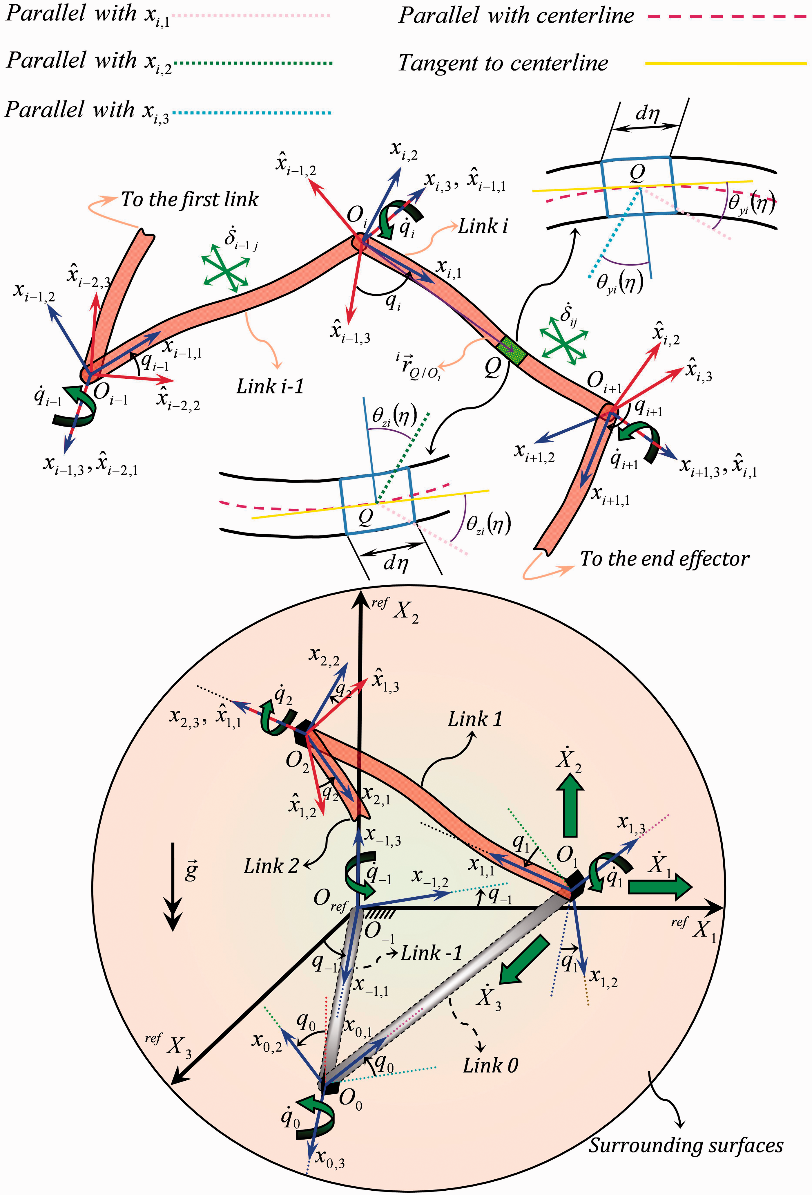
This section presents the kinematic modeling of a flexible-link robotic manipulator in 3D space, in which the links are connected via rigid, frictionless, revolute joints. Link $i - 1$ and Link i of this open kinematic chain are depicted in Figure 1. Two coordinate systems $(x i, 1 x i, 2 x i, 3, x^i, 1 x^i, 2 x^i, 3)$ are attached to each link according to the following guidelines: $x i, 1 x i, 2 x i, 3$ is the coordinate system for Link i, whose origin is located at the beginning of this link; the $x i, 1$ axis is along the length of undeformed Link i (from O_i to $O i + 1$ ), the $x i, 3$ axis is along the joint axis (about which Link i rotates relative to Link $i - 1$ ), and $x i, 2$ completes the right-handed coordinate system. Also, $x^i, 1 x^i, 2 x^i, 3$ is the coordinate system whose origin is attached to the end of Link i and its orientation is exactly the same as that of the $x i, 1 x i, 2 x i, 3$ coordinate system, when Link i has no deformation. Also, $ref X 1 ref X 2 ref X 3$ is an inertial reference frame attached to the ground as a global coordinate system. Here, it is assumed that the first body’s local coordinate system, i.e. O₁, is not fixed to the ground and can easily move through the space. So, the displacements of this joint in the $ref X 1$ , $ref X 2$ and $ref X 3$ directions can be represented by X₁, X₂ and X₃, respectively. Moreover, the absolute velocities of this joint with respect to the global coordinate system are denoted by $X \cdot j$ , where $j = 1, 2, 3$ . Except the first link, all the other links in this robotic system possess only one rotational degree of freedom. The first link, as a suspended body that can move freely through the space, has three rotational degrees of freedom; so, it can be modeled as three joints ( $O - 1$ ,O₀ and O₁) of one DOF connected to two imaginary links of zero length (Link ( $- 1$ ) and Link ( $0$ )). Therefore, only the manipulators with one rotational DOF will be considered. The parameter of the number of mode shapes m_i has been used to model the elastic properties of Link i. Hence, the degree of freedom (DOF) of the system is expressed as $DOF = n + \sum_{i = 1}^{n} m i + 5$ , where $n + 2$ degrees of freedom are associated with the orientation of links $(q i)$ , $\sum_{i = 1}^{n} m i$ degrees of freedom are associated with the flexural displacements of links $(δ ij)$ , and the other three degrees of freedom concern the position of the first joint with respect to the global coordinate system $(X j)$ .

Let us consider an arbitrary differential element, Q, on Link i. The position of this differential element with respect to the $x i, 1 x i, 2 x i, 3$ coordinate system includes a rigid and an elastic part, as follows:

i r \to Q / O i = \underset{Rigid}{\underset{︸}{η \to i}} + \underset{Elastic}{\underset{︸}{\sum_{j = 1}^{m i} δ ij (t) r \to ij (η)}}

(1)

η \to i = {η i 001} T

is the position vector of differential element Q with respect to O_i when link i has no deformation. Also,

r \to ij = {x 1 ij x 2 ij x 3 ij 0} T

is the Eigenfunction vector whose components (

x 1 ij

x 2 ij

and

x 3 ij

) are the jth longitudinal and bending mode shapes of Link i, and

δ ij

is the jth time-dependent modal generalized coordinate of Link i. Moreover, the rotation of this differential element can be represented by means of a truncated modal expansion as

i θ \to i = \sum_{j = 1}^{m i} δ ij (t) θ \to ij (η)

(2)

where

θ \to ij = {θ x 1 ij θ x 2 ij θ x 3 ij} T

is the Eigenfunction vector whose components (

θ x 1 ij

θ x 2 ij

and

θ x 3 ij

) are the jth rotational mode shapes of Link i in the

O i x i, 1

O i x i, 2

and

O i x i, 3

directions, respectively.

The position vector of differential element Q from Link i can be represented in any coordinate system j if the transformation matrix $j T i$ is known.

j T i = [j R i 0 \to T | j {x \to}_{j, 1}^{T} \cdot j r \to O i / O j j {x \to}_{j, 2}^{T} \cdot j r \to O i / O j j {x \to}_{j, 3}^{T} \cdot j r \to O i / O j 1]

(3)

where

j R i

is the rotation matrix that demonstrates the orientation of the

x i, 1 x i, 2 x i, 3

coordinate system with respect to

x j, 1 x j, 2 x j, 3

;

j r \to O i / O j

is the position vector of O_i with respect to O_j which is expressed in coordinate system j; and

j x \to j, 1 = {1000} T

j x \to j, 2 = {0100} T

j x \to j, 3 = {0010} T

and

0 \to = {000} T

. Now, the position of Q with respect to the reference coordinate system can be specified as

ref r \to Q / O ref = ref T i i r \to Q / O i = T i i r \to Q / O i

(4)

Since the approach developed in this manuscript is based on the Gibbs-Appell formulation, the absolute acceleration of differential element Q is required. This acceleration can be expressed as

ref \to ·· r Q / O ref = T ·· i i r \to Q / O i + 2 T \cdot i i \to \cdot r Q / O i + T i i \to ·· r Q / O i

(5)

In the above equation, T_i can be represented recursively as

T i = T i - 1 E i - 1 A i

(6)

where A_i is defined as the joint’s transformation matrix, which demonstrates the orientation of the

x i, 1 x i, 2 x i, 3

coordinate system with respect to

x^i - 1, 1 x^i - 1, 2 x^i - 1, 3

; and E_i is the link’s transformation matrix, which shows the orientation and translation of the

x^i, 1 x^i, 2 x^i, 3

coordinate system with respect to

x i, 1 x i, 2 x i, 3

. These two matrices can be written as

A i = [x i, 1 \cdot x^i - 1, 1 x i, 2 \cdot x^i - 1, 1 x i, 3 \cdot x^i - 1, 1 0 x i, 1 \cdot x^i - 1, 2 x i, 2 \cdot x^i - 1, 2 x i, 3 \cdot x^i - 1, 2 0 x i, 1 \cdot x^i - 1, 3 x i, 2 \cdot x^i - 1, 3 x i, 3 \cdot x^i - 1, 3 00001] i = - 1 \dots . n

(7)

E i = \underset{Rigid}{\underset{︸}{H i}} + \underset{Elastic}{\underset{︸}{\sum_{j = 1}^{m i} δ ij (t) M ij}} i = 1 \dots . n

(8)

where

H i = [100 l i 010000100001]

(9)

The first and second time derivatives of A_i and E_i appear in equation (5). These four terms can be represented as

A \cdot i = \frac{\partial A i}{\partial q i} q \cdot i = U 1 i q \cdot i

(11)

A ·· i = \frac{\partial 2 A i}{\partial q_{i}^{2}} {q \cdot}_{i}^{2} + \frac{\partial A i}{\partial q i} q ·· i = U 2 i {q \cdot}_{i}^{2} + U 1 i q ·· i

(12)

E \cdot i = H \cdot i + \sum_{j = 1}^{m i} δ \cdot ij (t) M ij

(13)

E ·· i = H ·· i + \sum_{j = 1}^{m i} δ ·· ij (t) M ij

(14)

Since the links have constant lengths (l_i), the values of

H \cdot i

and

H ·· i

are zero for all the links. To insert the distance between Points O₁ and

O ref

into the formulations, the

E - 2

transformation matrix is introduced.

E - 2 = [100 X 1 010 X 2 001 X 3 0001]

(15)

Now, the first and second time derivatives of

E - 2

can be represented as

E \cdot - 2 = \sum_{i = 1}^{3} \frac{\partial E - 2}{\partial X i} X \cdot i = \sum_{i = 1}^{3} U 3 i X \cdot i

(16)

E ·· - 2 = \sum_{i = 1}^{3} U 3 i X ·· i

(17)

In the next section, equation (5) will be used to obtain the acceleration energy (Gibbs function) of the whole system.

3. Dynamics of the system

3.1. Flight phase

In the flight phase, there is no contact between the manipulator and the surrounding walls and the differential equations in this phase can be obtained by the Gibbs-Appell formulation, in which the acceleration and potential energies of each link are calculated first, and then theses partial terms are added together to get the total acceleration energy (S) and total potential energy (V).

The acceleration energy (Gibbs function) of a robotic manipulator which consists of n real flexible links with length l_i can be represented as

S = \sum_{i = 1}^{n} \int_{0}^{l i} [\frac{1}{2} μ i (η i) Tr (ref \to ·· r Q / O ref \cdot ref \to ·· r_{Q / O ref}^{T}) + \frac{1}{2} i \to \cdot ω_{i}^{T} \cdot J' i (η i) i \to \cdot ω i + i \to \cdot ω_{i}^{T} \cdot i ω \sim i J' i (η i) i ω \to i] d η i

(18)

where

i ω \sim i

is the skew symmetric tensor related to vector

i ω \to i

. As seen in equation (18), the mass per unit length and the mass moment of inertia per unit length of Link i (i.e.,

μ i (η i)

and

J' i (η i)

) are not necessarily distributed uniformly along the links. Note that the links in flexible robotic manipulators are usually assumed to be very slender. So, it is justifiable to ignore the second and third terms in equation (18). By inserting equation (5) into equation (18) we get

S = \sum_{i = 1}^{n} Tr {T ·· i B 5 i {T ··}_{i}^{T} + 4 T ·· i B 4 i {T \cdot}_{i}^{T} + 2 T ·· i B 3 i T_{i}^{T} + 4 T \cdot i B 2 i T_{i}^{T} + T i B 1 i T_{i}^{T}} + irrelevant terms

(19)

where

B 1 i = \sum_{k = 1}^{m i} \sum_{j = 1}^{m i} δ ·· ik δ ·· ij C 1 ikj

(20)

B 2 i = \sum_{k = 1}^{m i} \sum_{j = 1}^{m i} δ \cdot ik δ ·· ij C 1 ikj

(21)

B 3 i = \sum_{j = 1}^{m i} δ ·· ij C 2 ij + \sum_{k = 1}^{m i} \sum_{j = 1}^{m i} δ ik δ ·· ij C 1 ikj

(22)

B 4 i = \sum_{j = 1}^{m i} δ \cdot ij C 2 ij + \sum_{k = 1}^{m i} \sum_{j = 1}^{m i} δ ik δ \cdot ij C 1 ikj

(23)

B 5 i = C 3 i + \sum_{j = 1}^{m i} δ ij (C 2 ij + C_{2 ij}^{T}) + \sum_{k = 1}^{m i} \sum_{j = 1}^{m i} δ ik δ ij C 1 ikj

(24)

And also

C 1 ikj

C 2 ij

and

C 3 i

can be represented as

C 1 ikj = \frac{1}{2} \int_{0}^{l i} μ i (η i) r \to ik (η i) {r \to}_{ij}^{T} (η i) d η i

(25)

C 2 ij = \frac{1}{2} \int_{0}^{l i} μ i (η i) η \to i {r \to}_{ij}^{T} (η i) d η i

(26)

C 3 i = \frac{1}{2} \int_{0}^{l i} μ i (η i) η \to i {η \to}_{i}^{T} d η i

(27)

In the Gibbs-Appell method, the governing equations are obtained by differentiating the Gibbs function with respect to an independent set of quasi-accelerations. Here, the rotational motion of the joints (i.e., $q ·· j$ ), the flexural displacements of the links (i.e., $δ ·· jf$ ) and the translational motion of O₁ (i.e., $X ·· j$ ) are considered as the quasi-accelerations. All the other terms in the Gibbs function that do not have these coefficients can be discarded as the “irrelevant terms” (equation (19). Now, by taking the partial derivative of acceleration energy with respect to $q ·· j$ we will have

\frac{\partial S}{\partial q ·· j} = 2 \sum_{i = j}^{n} Tr {\frac{\partial T ·· i}{\partial q ·· j} [B 5 i {T ··}_{i}^{T} + 2 B 4 i {T \cdot}_{i}^{T} + B 3 i T_{i}^{T}]} j = - 1 \dots . n

(28)

Also, by taking the partial derivative of acceleration energy with respect to

δ ·· jf

we get

\frac{\partial S}{\partial δ ·· jf} = 2 \sum_{i = j + 1}^{n} Tr {\frac{\partial T ·· i}{\partial δ ·· jf} [B 5 i {T ··}_{i}^{T} + 2 B 4 i {T \cdot}_{i}^{T} + B 3 i T_{i}^{T}]} + 2 Tr {[T ·· j N jf + 2 T \cdot j \sum_{k = 1}^{m j} δ \cdot jk C 1 jkf + T j \sum_{k = 1}^{m j} δ ·· jk C 1 jkf] T_{j}^{T}} j = 1 \dots . . n; f = 1 \dots . . m j

(29)

where

N jf = C 2 jf + \sum_{k = 1}^{m j} δ jk C 1 jkf

(30)

And finally, the partial derivative of the Gibbs function with respect to

X ·· j

can be expressed as

\frac{\partial S}{\partial X ·· j} = 2 \sum_{i = 1}^{n} Tr {\frac{\partial T ·· i}{\partial X ·· j} [B 5 i {T ··}_{i}^{T} + 2 B 4 i {T \cdot}_{i}^{T} + B 3 i T_{i}^{T}]} j = 1 \dots . 3

(31)

Gravity and elastic deformation are two sources of potential energy for this flying and flexible multi-link system. The gravitational potential energy of the flexible links can be represented as

V g = - g \to T \cdot \sum_{i = 1}^{n} T i i r \to i

(32)

where

g \to

is the vector of the gravitational field and

i r \to i

is defined as

i r \to i = C \to 4 i + \sum_{k = 1}^{m i} δ ik C \to 5 ik

(33)

where

C \to 4 i = \int_{0}^{l i} μ i (η i) η \to d η i

(34)

C \to 5 ik = \int_{0}^{l i} μ i (η i) r \to ik (η i) d η i

(35)

As is shown in Korayem and Shafei (2013), the strain potential energy for an n-elastic-link robotic manipulator can be expressed as

V e = \frac{1}{2} \sum_{i = 1}^{n} \sum_{j = 1}^{m i} \sum_{k = 1}^{m i} δ ij (t) δ ik (t) K ijk

(36)

where

K ijk = \int_{0}^{l i} [G i (η i) I x 1 i (η i) \frac{\partial θ x 1 ij}{\partial η i} \frac{\partial θ x 1 ik}{\partial η i} + E' i (η i) A' i (η i) \frac{\partial x 1 ij}{\partial η i} \frac{\partial x 1 ik}{\partial η i} + E' i (η i) I x 2 i (η i) \frac{\partial θ x 2 ij}{\partial η i} \frac{\partial θ x 2 ik}{\partial η i} + E' i (η i) I x 3 i (η i) \frac{\partial θ x 3 ij}{\partial η i} \frac{\partial θ x 3 ik}{\partial η i}] d η i

(37)

I x 1 i

I x 2 i

and

I x 3 i

are the area moments of inertia about the

O i x i, 1

O i x i, 2

and

O i x i, 3

axes, respectively, and

A' i

is the cross-sectional area of the ith link. According to equation (37), the elastic properties of the system [i.e., Young’s modules (

E' i (η i)

) and shear modules (

G i (η i)

)] could be expressed as a function of link length. The total potential energy of the system can be obtained by summing equations (32) and (36). To derive the conservative generalized forces arising from the gravity and elastic deformations, the partial derivatives of potential energy with respect to quasi-coordinates are needed.

\frac{\partial V}{\partial q j} = - g \to T \cdot \sum_{i = j}^{n} \frac{\partial T i}{\partial q j} i r \to i j = - 1 \dots . n

(38)

\frac{\partial V}{\partial δ jf} = - g \to T \cdot (T j C \to 5 jf + \sum_{i = j + 1}^{n} \frac{\partial T i}{\partial δ jf} i r \to i) + \sum_{k = 1}^{m j} δ jk (t) K jkf j = 1 \dots . . n; f = 1 \dots . . m j

(39)

\frac{\partial V}{\partial X j} = - g \to T \cdot \sum_{i = 1}^{n} (\frac{\partial T i}{\partial X j} i r \to i) j = 1 \dots . 3

(40)

3.1.1. Inverse dynamics

The system’s motion equations will be completed by considering the external forces or torques that are applied on the links or joints. Here, it has been assumed that there are no loads on the links and no torques on the joints. With this assumption, the differential motion equations of nelastic links, in the flight phase, can be expressed as follows:

The rotational motion equation of the jth joint in the flight phase:

\frac{\partial S}{\partial q ·· j} + \frac{\partial V}{\partial q j} = 0 j = - 1 \dots . n

(41)

The fth vibrational motion equation of the jth link in the flight phase:

\frac{\partial S}{\partial δ ·· jf} + \frac{\partial V}{\partial δ jf} = 0 j = 1 \dots . . n; f = 1 \dots . . m

(42)

The jth translational motion equation of the first joint (O₁) in the flight phase:

\frac{\partial S}{\partial X ·· j} + \frac{\partial V}{\partial X j} = 0 j = 1 \dots . 3

(43)

For the computer simulation of the abovementioned robotic system, the inverse dynamic form of the motion equations (equations (41)-(43)) should be converted to the forward dynamic form.

3.1.2. Forward dynamics

The governing equations derived in the preceding section are expressed in the dynamic form as

I f (Θ) \to ·· Θ = Re (Θ, Θ \cdot)

(44)

where

I f (Θ)

is the inertia matrix of the system in the flight phase, which is symmetric and positive-definite. Also

\to ·· Θ

(the quasi-acceleration vector) and

Re (Θ, Θ \cdot)

(the remaining dynamics terms containing Coriolis and centrifugal forces) can be represented as

\to ·· Θ = {q ·· - 1 q ·· 0 q ·· 1 δ ·· 11 \dots δ ·· 1 m q ·· 2 δ ·· 21 \dots δ ·· 2 m \dots q ·· n δ ·· n 1 \dots δ ·· nm X ·· 1 X ·· 2 X ·· 3} T

(45)

Re (Θ, Θ \cdot) = {Re q - 1 Re q 0 Re q 1 Re δ 11 \dots Re δ 1 m Re q 2 Re δ 21 \dots Re δ 2 m \dots Re q n Re δ n 1 \dots Re δ nm Re X 1 Re X 2 Re X 3} T

(46)

To achieve the objective of this section, the partial derivatives of T_i and $T ·· i$ with respect to quasi-coordinates and quasi-accelerations, which appeared in previous equations, should be evaluated. Let us express T_i in two different forms.

T i = A - 2 E - 2 A - 1 E - 1 A 0 E 0 A 1 E 1 \dots . . A h E h \dots . E i - 1 A i = T^h - 1 A h h T \sim i = T h E h h T i

(47)

Note that

A - 2

E - 1

and E₀ are the identity matrices that are inserted into the T_i transformation matrix to ensure an organized arrangement. By taking the second derivative of T_i with respect to time and changing the outcome to a summation form, we get

T ·· i = T ·· s, i + T ·· v, i

(48)

where

T ·· s, i

represent those terms of

T ·· i

that include the quasi-accelerations; while

T ·· v, i

denote those terms of

T ·· i

that do not have

q ·· j

δ ·· jf

and

X ·· j

as quasi-accelerations. These two terms can be expressed as

T ·· s, i = \sum_{k = - 1}^{i} T^k - 1 U 1 k k T \sim i q ·· k + \sum_{k = 1}^{i - 1} \sum_{t = 1}^{m k} T k M kt k T i δ ·· kt + \sum_{k = 1}^{3} T - 2 U 3 k - 2 T i X ·· k

(49)

T ·· v, i = \sum_{k = - 1}^{i} (^\cdot T k - 1 U 1 k k T \sim i + T^k - 1 U 2 k k T \sim i q \cdot k + T^k - 1 U 1 k k \sim \cdot T i) q \cdot k + \sum_{k = 1}^{i - 1} (\sum_{t = 1}^{m k} T \cdot k M kt k T i + T k M kt k T \cdot i) δ \cdot kt + \sum_{k = 1}^{3} (T \cdot - 2 U 3 k - 2 T i + T - 2 U 3 k - 2 T \cdot i) X \cdot k

(50)

Now, the partial derivatives of T_i and

T ·· i

with respect to quasi-coordinates and quasi-accelerations can be evaluated as

\frac{\partial T ·· i}{\partial q ·· j} = \frac{\partial T i}{\partial q j} = T^j - 1 U 1 j j T \sim i

(51)

\frac{\partial T ·· i}{\partial δ ·· jf} = \frac{\partial T i}{\partial δ jf} = T j M jf j T i

(52)

\frac{\partial T ·· i}{\partial X ·· j} = \frac{\partial T i}{\partial X j} = T - 2 U 3 j - 2 T i

(53)

To construct the inertia matrix of the whole system, it is necessary to insert equations (51) – (53) and also equations (49)–(50) into the relevant parts of equations (41) - (43). Then, all the terms that contain $q ·· k$ , $δ ·· kt$ and $X ·· k$ should be maintained on the left hand side of the equal sign and all the remaining terms containing the Coriolis and centrifugal forces should be transferred to the right hand side. By placing the left hand side terms of the governing equations in a matrix form, the inertia matrix of this flying open kinematic chain can be obtained. The details of this procedure are presented below.

The coefficients of quasi-accelerations in the rotational motion equations: In equation (41), all the terms that include $q ·· k$ , $δ ·· kt$ and $X ·· k$ as their coefficients can be grouped as

\sum_{k = - 1}^{n} \underset{1}{\underset{︸}{2 Tr {T^j - 1 U 1 j j F \sim k U_{1 k}^{T} {T^}_{k - 1}^{T}}}} q ·· k + (\sum_{k = 1}^{n - 1} \sum_{t = 1}^{m k} \underset{2}{\underset{︸}{2 Tr {T^j - 1 U 1 j j F k M_{kt}^{T} T_{k}^{T}}}} + \sum_{k = max (1, j)}^{n} \sum_{t = 1}^{m k} \underset{3}{\underset{︸}{2 Tr {T^j - 1 U 1 j j T \sim k N kt T_{k}^{T}}}}) δ ·· kt + \sum_{k = n + 1}^{n + 3} \underset{4}{\underset{︸}{2 Tr {T^j - 1 U 1 j j F - 2 U_{3 (k - n)}^{T} T_{- 2}^{T}}}} X ·· k - n j = - 1 \dots . n

(I)

where

j F \sim k = \sum_{i = max (1, k, j)}^{n} j T \sim i B 5 i k {T \sim}_{i}^{T}

(54)

j F k = \sum_{i = max (k + 1, j)}^{n} j T \sim i B 5 i k T_{i}^{T}

(55)

j F - 2 = \sum_{i = max (1, j)}^{n} j T \sim i B 5 i - 2 T_{i}^{T}

(56)

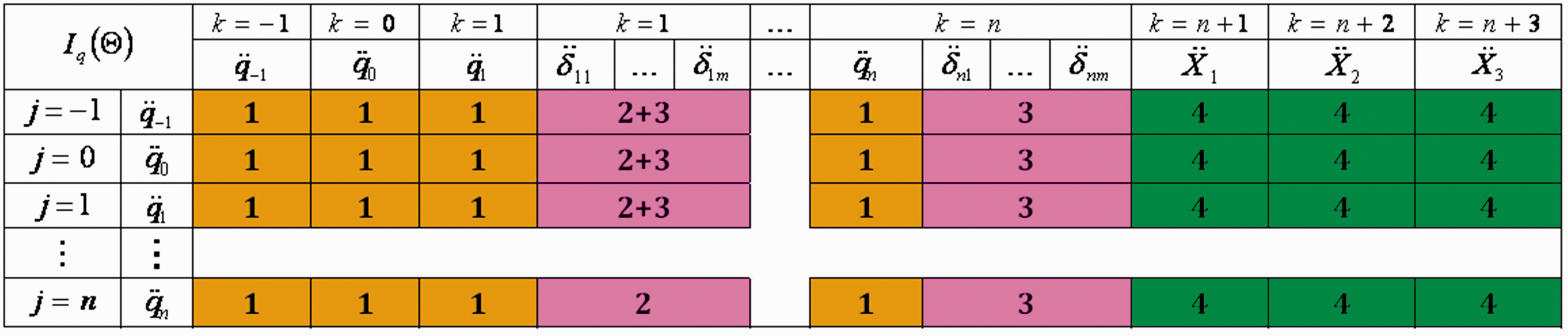
The constitutive terms of Exp. (I), numbered from (1) to (4), form the inertia matrix of the rotational motion equations (Figure 2).

Coriolis and centrifugal forces in the rotational motion equations: Now, let us construct the right hand sides of the rotational motion equations. In equation (41), if all the terms that do not contain $q ·· k$ , $δ ·· kt$ and $X ·· k$ are moved to the right hand side of the equal sign, the following equation will be obtained.

Re q j = \underset{5}{\underset{︸}{\sum_{i = max (1, j)}^{n} (g \to T \cdot \frac{\partial T i}{\partial q j} i r \to i - 2 Tr {\frac{\partial T ·· i}{\partial q ·· j} [B 5 i {T ··}_{v, i}^{T} + 2 B 4 i {T \cdot}_{i}^{T}]})}} j = - 1 \dots . n

(57)

The constitutive term of equation (57), which is numbered (5), forms the right hand side vector of the rotational motion equations (see Figure 3).

The coefficients of quasi-accelerations in the vibrational motion equations: In equation (42), all the terms that include $q ·· k$ , $δ ·· kt$ and $X ·· k$ as their coefficients can be grouped as

(\sum_{k = - 1}^{n} \underset{6}{\underset{︸}{2 Tr {T j M jf j F ¯ k U_{1 k}^{T} {T^}_{k - 1}^{T}}}} + \sum_{k = - 1}^{j} \underset{7}{\underset{︸}{2 Tr {T^k - 1 U 1 k k T \sim j N jf T_{j}^{T}}}}) q ·· k + (\sum_{k = 1}^{n - 1} \sum_{t = 1}^{m k} \underset{8}{\underset{︸}{2 Tr {T j M jf j F^k M_{kt}^{T} T_{k}^{T}}}} + \sum_{k = j + 1}^{n} \sum_{t = 1}^{m k} \underset{9}{\underset{︸}{2 Tr {T j M jf j T k N kt T_{k}^{T}}}} + \sum_{k = 1}^{j - 1} \sum_{t = 1}^{m k} \underset{10}{\underset{︸}{2 Tr {T k M kt k T j N jf T_{j}^{T}}}} + \sum_{t = 1}^{m j} \underset{11}{\underset{︸}{2 Tr {T j C 1 jtf T_{j}^{T}}}}) δ ·· kt + (\sum_{k = n + 1}^{n + 3} \underset{12}{\underset{︸}{2 Tr {T j M jf j F^- 2 U_{3 (k - n)}^{T} T_{- 2}^{T}}}} + \sum_{k = n + 1}^{n + 3} \underset{13}{\underset{︸}{2 Tr {T - 2 U 3 (k - n) - 2 T j N jf T_{j}^{T}}}}) X ·· k - n j = 1 \dots . . n = 1 \dots . . m

(II)

where

j F^k = \sum_{i = max (j + 1, k + 1)}^{n} j T i B 5 i k T_{i}^{T}

(58)

j F ¯ k = \sum_{i = max (j + 1, k)}^{n} j T i B 5 i k {T \sim}_{i}^{T}

(59)

j F^- 2 = \sum_{i = j + 1}^{n} j T i B 5 i - 2 T_{i}^{T}

(60)

The constitutive terms of Exp. (II), numbered from (6) to (13), form the inertia matrix of the vibrational motion equations (see Figure 4).

Coriolis and centrifugal forces in the vibrational motion equations: Like the previous step, in equation (42), all the terms that do not include the quasi-accelerations should be transferred to the right hand side of the equal sign, as follows:

Re δ jf = \underset{14}{\underset{︸}{- 2 Tr {[T ·· v, j N jf + 2 T \cdot j \sum_{k = 1}^{m j} δ \cdot jk C 1 jkf] T_{j}^{T}}}} + \underset{15}{\underset{︸}{\sum_{k = 1}^{m j} - δ jk (t) K jkf}} + \underset{16}{\underset{︸}{g \to T \cdot T j C \to 5 jf}} + \underset{17}{\underset{︸}{\sum_{i = j + 1}^{n} (g \to T \cdot \frac{\partial T i}{\partial δ jf} i r \to i - 2 Tr {\frac{\partial T ·· i}{\partial δ ·· jf} [B 5 i {T ··}_{v, i}^{T} + 2 B 4 i {T \cdot}_{i}^{T}]})}} j = 1 \dots . . n = 1 \dots . . m

(61)

The constitutive terms of equation (61), numbered from (14) to (17), form the right hand side vector of the vibrational motion equations, as is shown in Figure 5.

The coefficients of quasi-accelerations in the translational motion equations: Like the previous two steps, in equation (43), all the terms that contain $q ·· k$ , $δ ·· kt$ and $X ·· k$ should be grouped as

\sum_{k = - 1}^{n} \underset{18}{\underset{︸}{2 Tr {T - 2 U 3 j - 2 F ¯ k U_{1 k}^{T} {T^}_{k - 1}^{T}}}} q ·· k + (\sum_{k = 1}^{n - 1} \sum_{t = 1}^{m k} \underset{19}{\underset{︸}{2 Tr {T - 2 U 3 j - 2 F^k M_{kt}^{T} T_{k}^{T}}}} + \sum_{k = 1}^{n} \sum_{t = 1}^{m k} \underset{20}{\underset{︸}{2 Tr {T - 2 U 3 j - 2 T k N kt T_{k}^{T}}}}) δ ·· kt + \sum_{k = n + 1}^{n + 3} \underset{21}{\underset{︸}{2 Tr {T - 2 U 3 j - 2 F^- 2 U_{3 (k - n)}^{T} T_{- 2}^{T}}}} X ·· k - n j = 1 \dots . 3

(III)

where

- 2 F^- 2 = \sum_{i = 1}^{n} - 2 T i B 5 i - 2 T_{i}^{T}

(62)

- 2 F ¯ k = \sum_{i = max (1, k)}^{n} - 2 T i B 5 i k {T \sim}_{i}^{T}

(63)

- 2 F^k = \sum_{i = k + 1}^{n} - 2 T i B 5 i k T_{i}^{T}

(64)

The constitutive terms of Exp. (III), which are numbered from (18) to (21), form the inertia matrix of the translational motion equations (Figure 6).

Coriolis and centrifugal forces in the translational motion equations: Finally, in equation (43), if all the terms that do not include the quasi-accelerations are transferred to the right hand side of the equal sign, the following equation will be obtained.

Re X j = \underset{22}{\underset{︸}{\sum_{i = 1}^{n} (g \to T \cdot \frac{\partial T i}{\partial X j} i r \to i - 2 Tr {\frac{\partial T ·· i}{\partial X ·· j} [B 5 i {T ··}_{v, i}^{T} + 2 B 4 i {T \cdot}_{i}^{T}]})}} j = 1 \dots . 3

(65)

The constructive term of equation (65), which is numbered (22), forms the right hand side vector of the translational motion equations, as is shown in Figure 7.

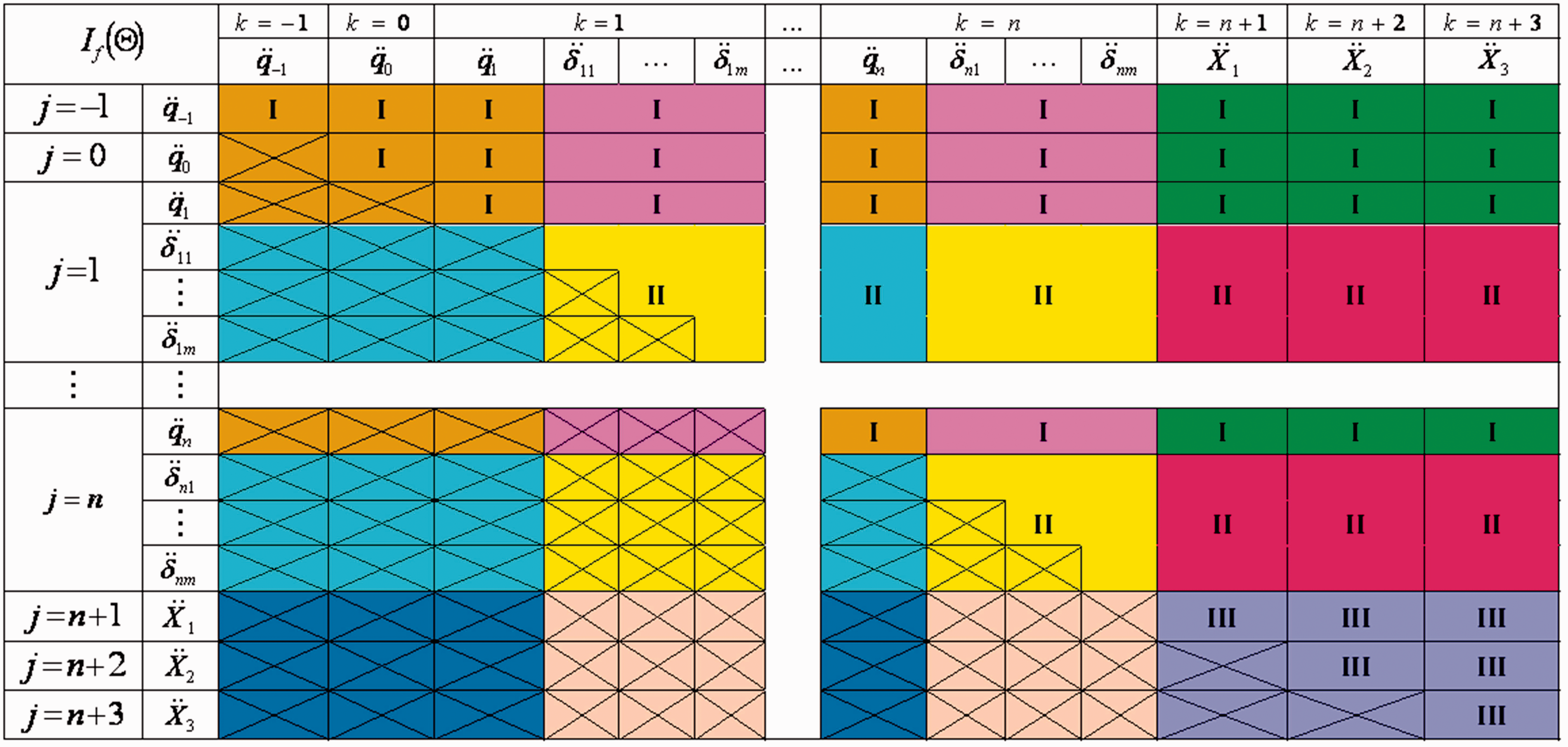
By integrating the inertia matrices for the rotational (Figure 2), vibrational (Figure 4) and translational (Figure 6) motion equations, the inertia matrix of the whole system in the flight phase will be obtained (see Figure 8). Since the inertia matrix of the whole system is symmetric, it is not necessary to evaluate the crossed out regions in Figure 8. This procedure, which is fully described in the Appendix, will greatly reduce the necessary computations.

Finally, by integrating the Coriolis and centrifugal forces into the rotational (Figure 3), vibrational (Figure 5) and translational (Figure 7) motion equations, the right hand side vector of the motion equations will be obtained (see Figure 9).

3.2. Impact phase

An impact occurs for the mentioned open kinematic chain when one of its joints touches the surfaces that surround the chain system. Before modeling the impact phase, let us present the absolute velocity of each joint in the inertial reference frame. Obviously, for an open kinematic chain which is composed of n flexible links, there are $n - 1$ joints and two end points (O₁ and O_n). By employing the Jacobian matrix, the velocities of these $n + 1$ points can be expressed as

ref \to \cdot r O i (Θ, Θ \cdot) = J i (Θ) \to \cdot Θ i = 1 \dots . . n + 1

(66)

The externally applied forces in an impact can be represented by impulses. So, the obtained equations in the previous section (flight phase), which include no external forces or torques, can be modified in the impact phase, as

I f (Θ) \to ·· Θ = Re (Θ, Θ \cdot) + J_{j}^{T} (Θ) ref n \to j δ F j (t)

(67)

where

ref n \to j

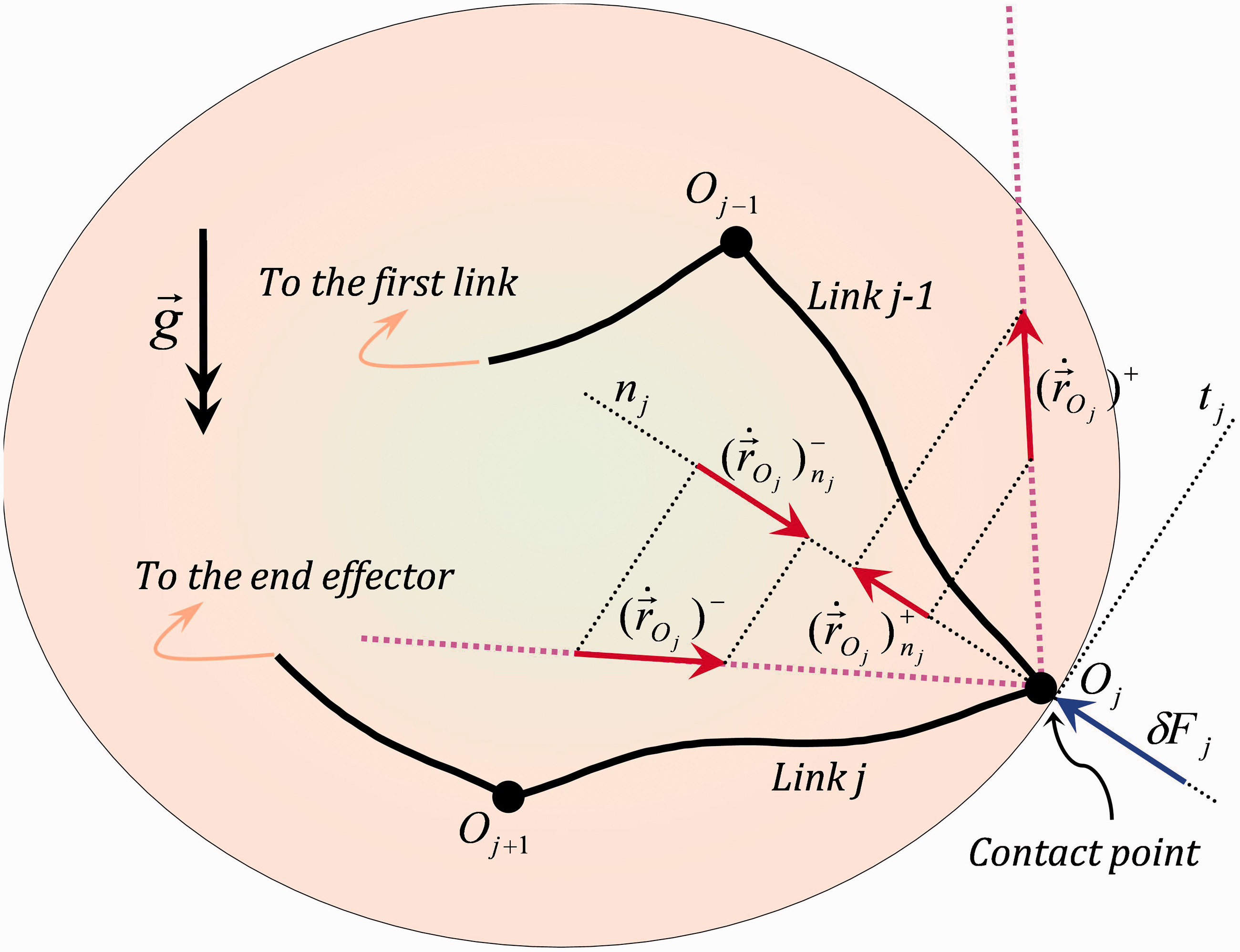
is a unit vector which is normal to the surface at the contact point, and expressed in the global coordinate system. Also,

δ F j (t)

represents the external force acting on the jth joint due to its collision with the curved wall (see Figure 10). As was pointed out, this force is impulsive; therefore, the

δ F j (t)

notation is used. If equation (67) is integrated over the infinitesimal duration of the impact time

(t - \to t +)

, the result will be

I f (Θ -) (\to \cdot Θ + - \to \cdot Θ -) = J_{j}^{T} (Θ -) ref n \to j F j j = 1 \dots . Num . ofContactPoints

(68)

where

F j = \int_{t -}^{t +} δ F j (t) d t

and also

\to \cdot Θ -

and

\to \cdot Θ +

are the quasi-velocities just before and just after an impact. In an impact, the configuration of a system is assumed not to change within a very short time interval; hence

Θ \to + = Θ \to -

. Finally, it should be noted that the values of

Re (Θ, Θ \cdot)

containing the Coriolis and centrifugal forces are finite; so, they vanish in the integration. Equation (68) represents

n + \sum_{i = 1}^{n} m i + 5

equations and

n + \sum_{i = 1}^{n} m i + 5 + \dim (F)

unknowns; where the unknowns are

\to \cdot Θ +

and F_j. So, it is required to find as many additional equations as the number of contact points. These additional equations are generated by knowing the relationship between the pre-collision and post-collision velocities of the impacting joints in n_j directions. Based on the Newton’s kinematic impact law, these equations can be written as

(ref \to \cdot r O j)_{n j}^{+} = - e (ref \to \cdot r O j)_{n j}^{-} \Rightarrow ref {n \to}_{j}^{T} \cdot J j (Θ -) \to \cdot Θ + = - e ref {n \to}_{j}^{T} \cdot J j (Θ -) \to \cdot Θ -

(69)

where e is called the coefficient of restitution. By combining Eqs. (68) and (69) we get

By multiplying both sides of equation (70) by

I_{i}^{- 1} (Θ)

the unknown variables (

\to \cdot Θ +

and F_j) will be determined. The final outcome of the impact phase becomes a new initial condition by which the flight phase model evolves until the next impact.

4. Computer simulations

Case study 1

In this section, two simulations are performed to validate the developed model. The first simulation involves a planar two-link flexible robotic manipulator, which is confined within a circle of $1 m$ radius (see Figure 11).

In order to have a planar motion in the $ref X 1 ref X 2$ plane, the initial conditions for $q - 1$ and q₀ should be $- \frac{π}{2} rad$ and $0 rad$ , respectively. In this plane, the system is released with the following initial conditions.

q 1 | t = 0 = - \frac{π}{6} rad; q 2 | t = 0 = - \frac{2 π}{3} rad; δ 11 = δ 21 | t = 0 = 0; X 1 | t = 0 = - 0.5 m; X 2 | t = 0 = - 0.4 m; X 3 | t = 0 = 0 m; q \cdot - 1 = q \cdot 0 = q \cdot 1 = q \cdot 2 | t = 0 = 0 \frac{rad}{s}; δ \cdot 11 = δ \cdot 21 | t = 0 = 0 \frac{1}{s}; X \cdot 1 = X \cdot 2 = X \cdot 3 | t = 0 = 0 \frac{m}{s};

To model the elastic deformations of each link, its first mode shape has been used along with clamped-clamped boundary conditions based on the EBBT approach (in which the mode shapes of deflections and rotations are related to each other). These bending and rotational mode shapes can be expressed as

x 211 = x 221 = \sin (4.73 η) - 1.017 \cos (4.73 η) - \sinh (4.73 η) + 1.017 \cosh (4.73 η)

(71)

θ x 311 = θ x 321 = \frac{dx 211}{d η} = \frac{dx 221}{d η}

(72)

All the other necessary parameters for the simulations can be found in Table 1.

Table 1.

Required parameters for simulating the planar motion of a two-flexible-link chain.

Parameters	Value	Unit
Length of the links	$l - 1 = l 0 = 0; l 1 = l 2 = 1;$	m
Mass per unit length	$μ - 1 = μ 0 = 0; μ 1 = μ 2 = 1;$	$kg \cdot m - 1$
Bending stiffness	$E' - 1 I x 3 - 1 = E' 0 I x 30 = 0;$ $E' 1 I x 31 = E' 2 I x 32 = 1000$	$N . m 2$
Gravity	$g = 9.81$	$m \cdot s - 2$
Coefficient of restitution	$e = 1$	–

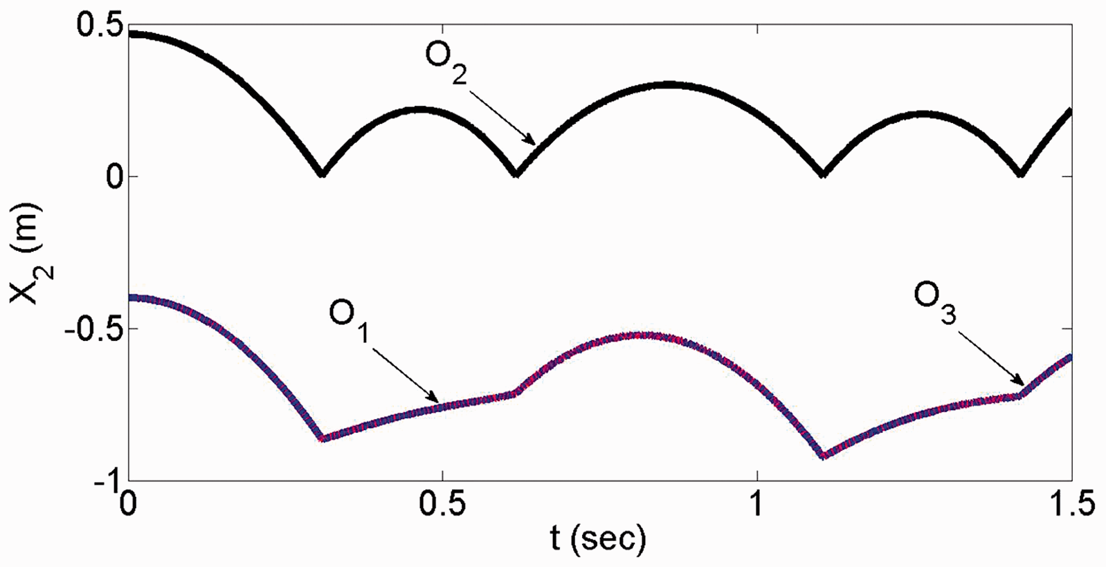
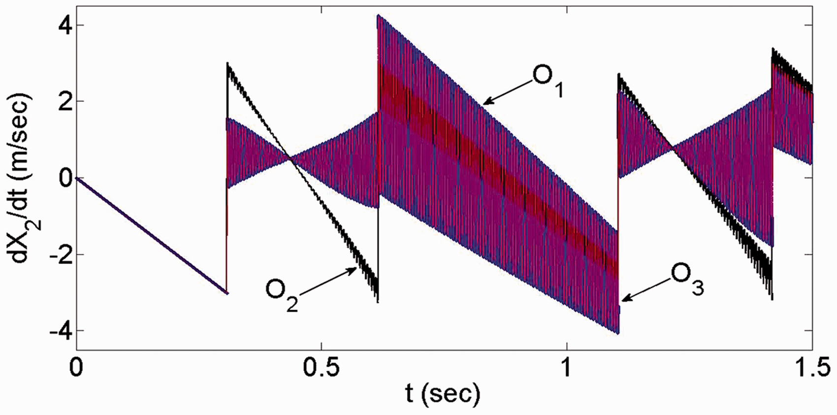
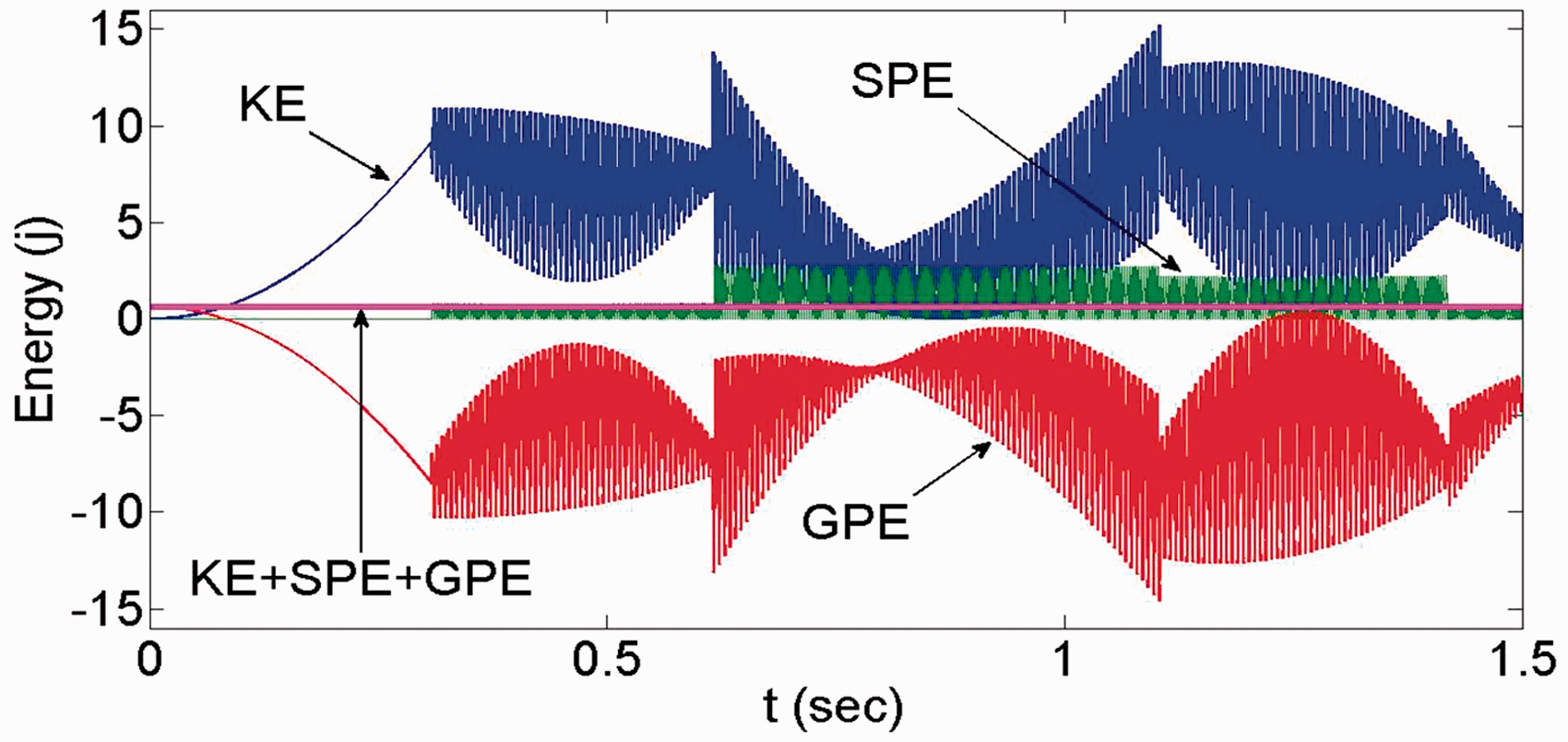
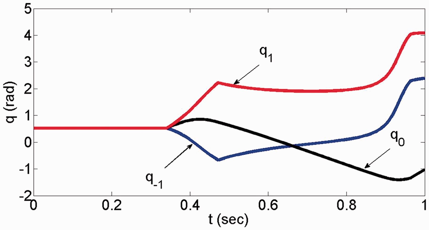
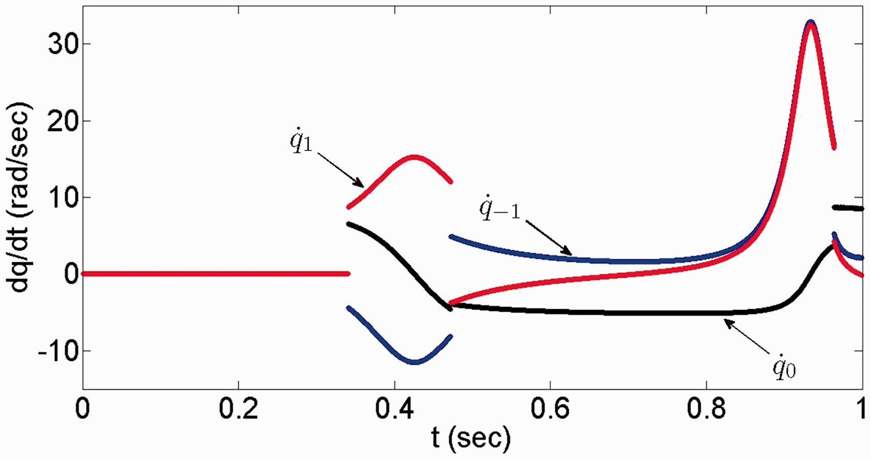
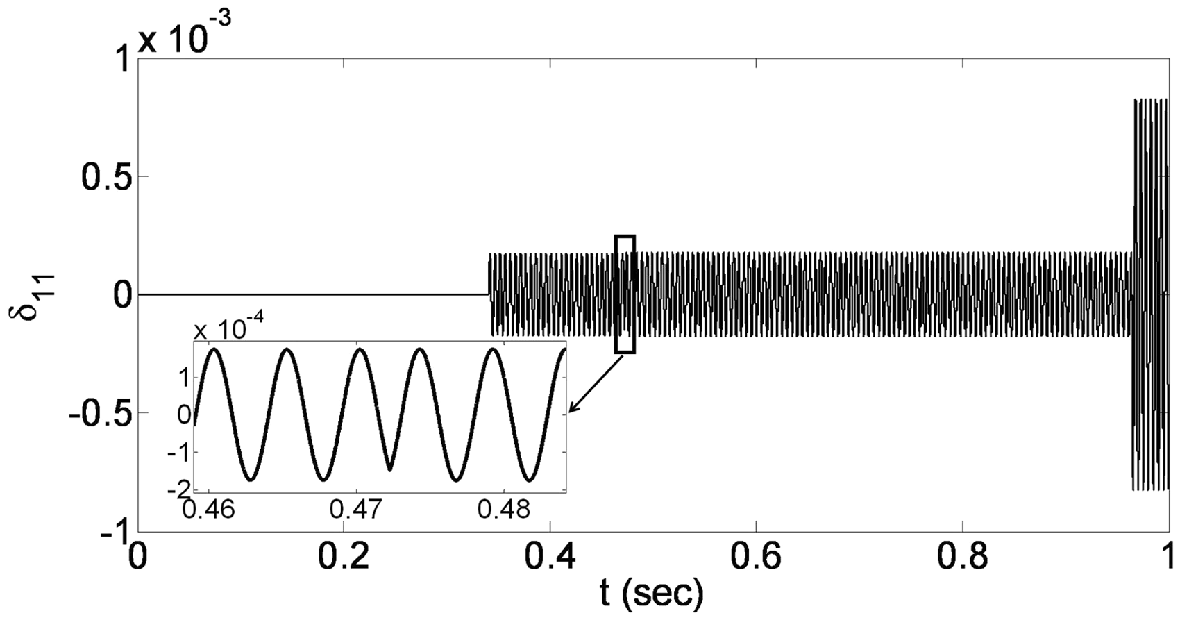
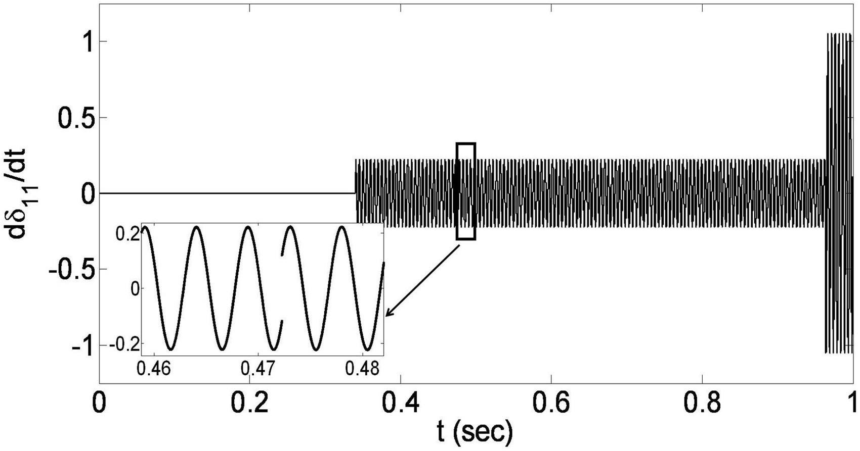
By solving a set of eighteen differential equations for the flight phase as well as the algebraic equations related to the system’s collision with the curved walls, the time responses, configurations and the energy history (i.e., kinetic, gravitational and strain potential energies) of this two-flexible-link flying robotic manipulator at different times are obtained and illustrated in Figure (12) through (21).

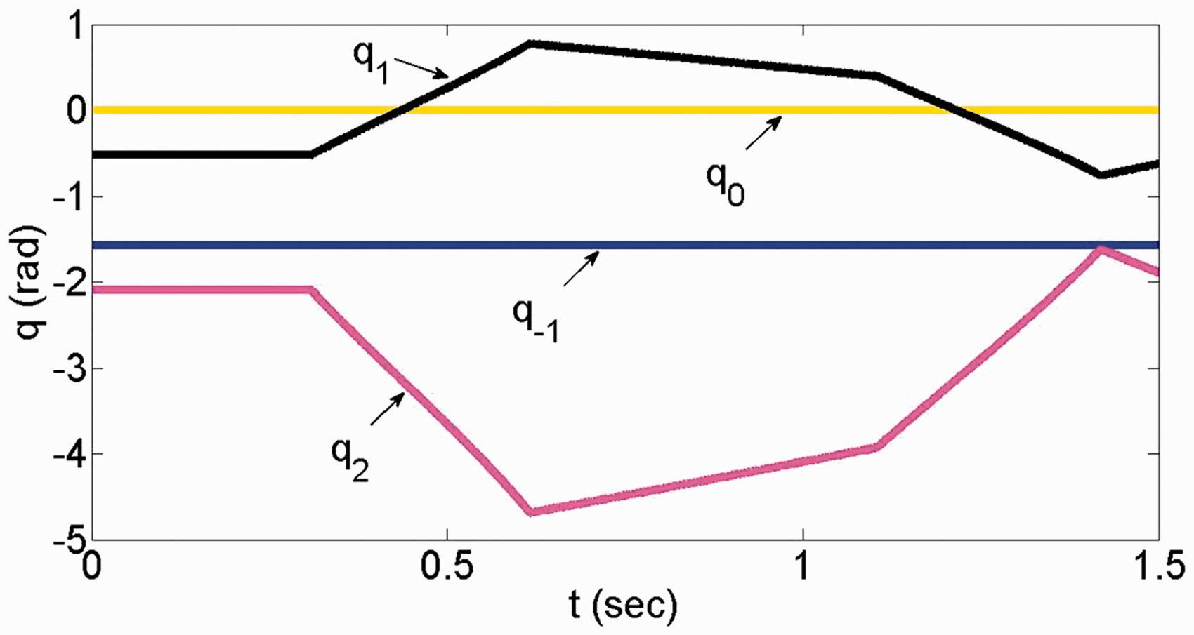
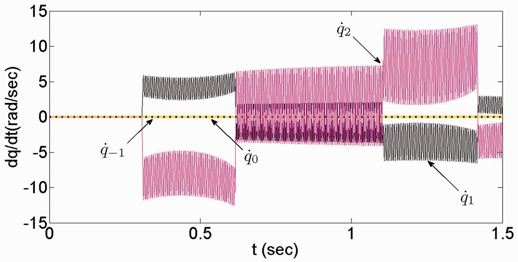
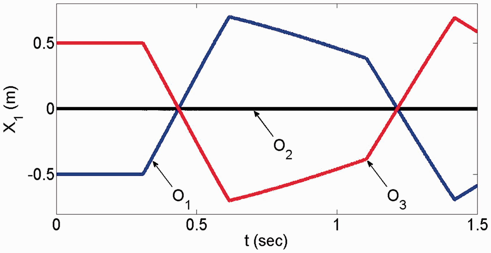
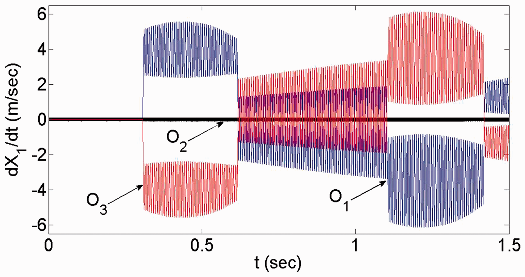
The initial conditions are deliberately chosen in such a way that the system has a symmetrical configuration with respect to $X 1 = 0 m$ . So, obviously, the system preserves its symmetricity during the simulation. Figures 12 and 13 respectively show the angular positions and velocities of the joints. Based on the system’s geometry (Figure 11), and according to the mentioned figures, relations $2 q 1 + q 2 = - π$ and $q \cdot 1 = - 0.5 q \cdot 2$ hold true for this simulation. Also, due to the symmetry of the system, the flexural displacements of the links and their variations with time are exactly the same (Figures 14 and 15). As shown in Figure 21, the system touches the boundary of the circle at four different times; $t = 0.308 s, 0.616 s, 1.105 s$ and $1.419 s$ . At these impact moments, the configuration of the system remains unchanged (i.e., $Θ \to - = Θ \to +$ ). This fact can be verified in Figures 12, 14, 16 and 18, where the values of the quasi-coordinates before and after the impacts are equal. However, the quasi-velocities quickly change at the moments of impact, as shown in Figures 13, 15, 17 and 19. Since there is no energy dissipation in the mentioned robotic system, it can be considered as a conservative system. So, it is reasonable to expect the total energy of the system to remain constant during the simulation. This is demonstrated in Figure 20, which shows the energy history of the system by illustrating the kinetic energy (KE), gravitational potential energy (GPT), strain potential energy (SPE), and the sum total of these energies for the examined system. According to this figure, the total energy of the system remains constant during the simulation at $0.6477 J$ . This validates the obtained equations and their solutions.

Case study 2

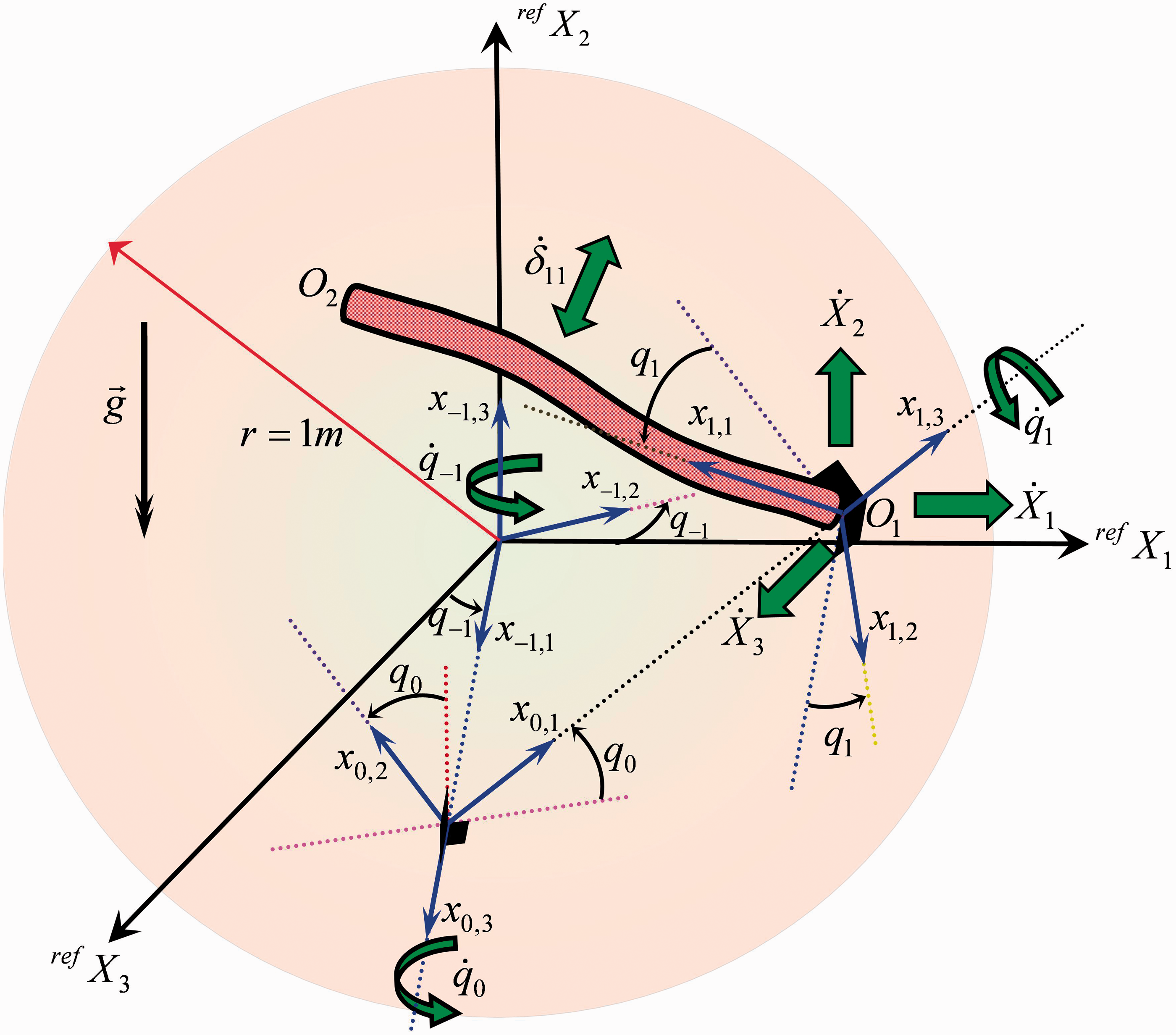
In the previous simulation, the confined system only had a planar motion. But here, a single flexible link with 3D spatial motion inside a closed sphere is considered (Figure 22).

The necessary parameters for the numerical simulations are presented in Table 2.

Table 2.

Required parameters for simulating a single flexible link confined within a sphere.

Parameters	Value	Unit
Length of the link	$l - 1 = l 0 = 0; l 1 = 1$	m
Mass per unit length	$μ - 1 = μ 0 = 0; μ 1 = 1$	$kgm - 1$
Bending stiffness	$E' - 1 I x 3 - 1 = E' 0 I x 30 = 0;$ $E' 1 I x 21 = E' 1 I x 31 = 1000$	$N . m 2$
Gravity	$g = 9.81$	$ms - 2$
Coefficient of restitution	$e = 1$	–

In this spatial dynamic system, the link vibrates in all directions. So, there will be two modes corresponding to each bending deflection pattern along the link: one in the $O 1 x 1, 2$ direction and the other in the $O 1 x 1, 3$ direction. If the link is completely axisymmetric, these two modes will have identical natural frequencies. Like the previous simulation, the first mode shapes of the Clamped-Clamped EBBT in both directions are considered as:

x 211 = x 311 = \sin (4.73 η) - 1.017 \cos (4.73 η) - \sinh (4.73 η) + 1.017 \cosh (4.73 η)

(73)

θ x 311 = \frac{dx 211}{d η}

(74)

θ x 211 = - \frac{dx 311}{d η}

(75)

Also the initial conditions are set as follows:

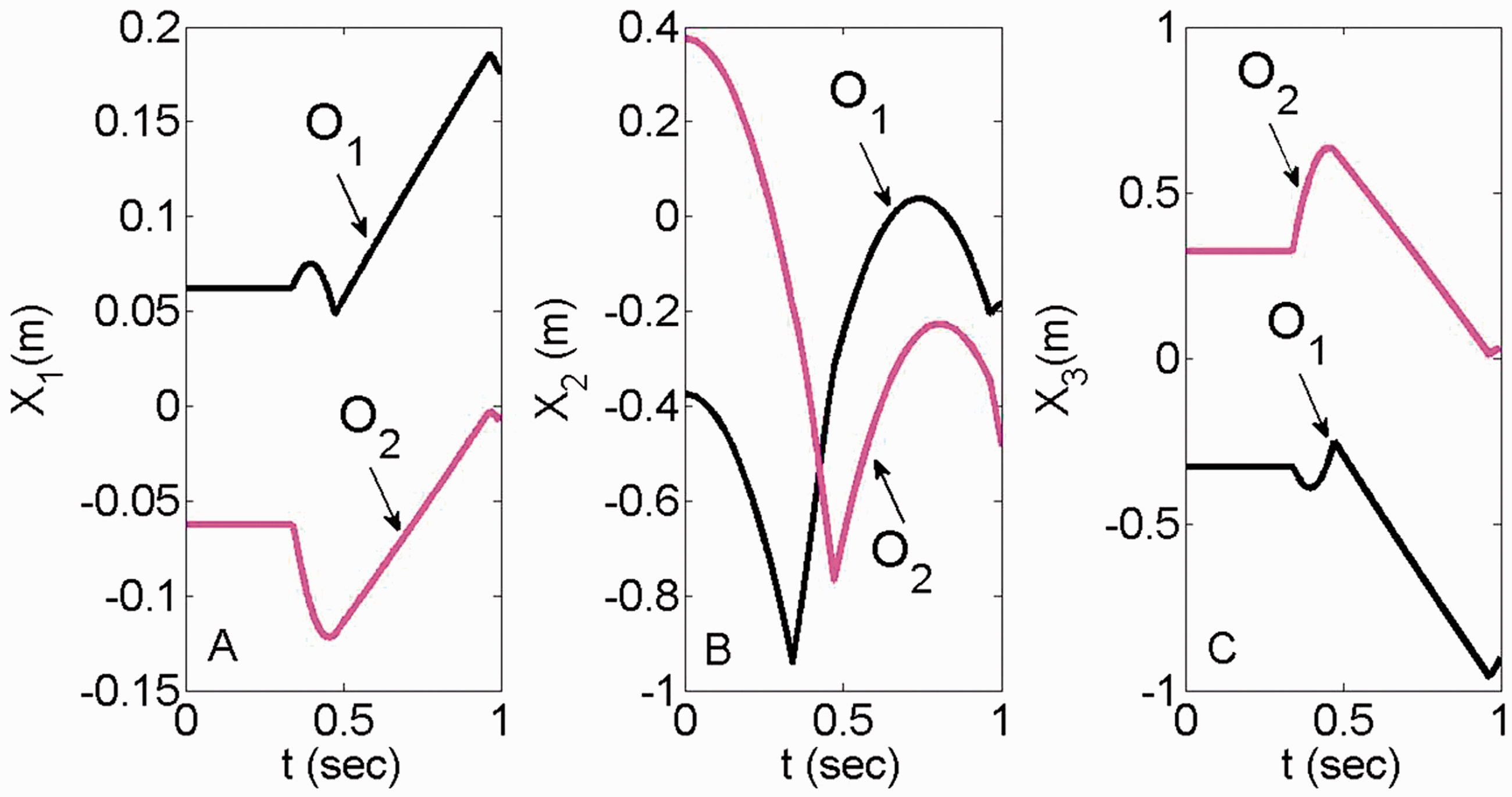
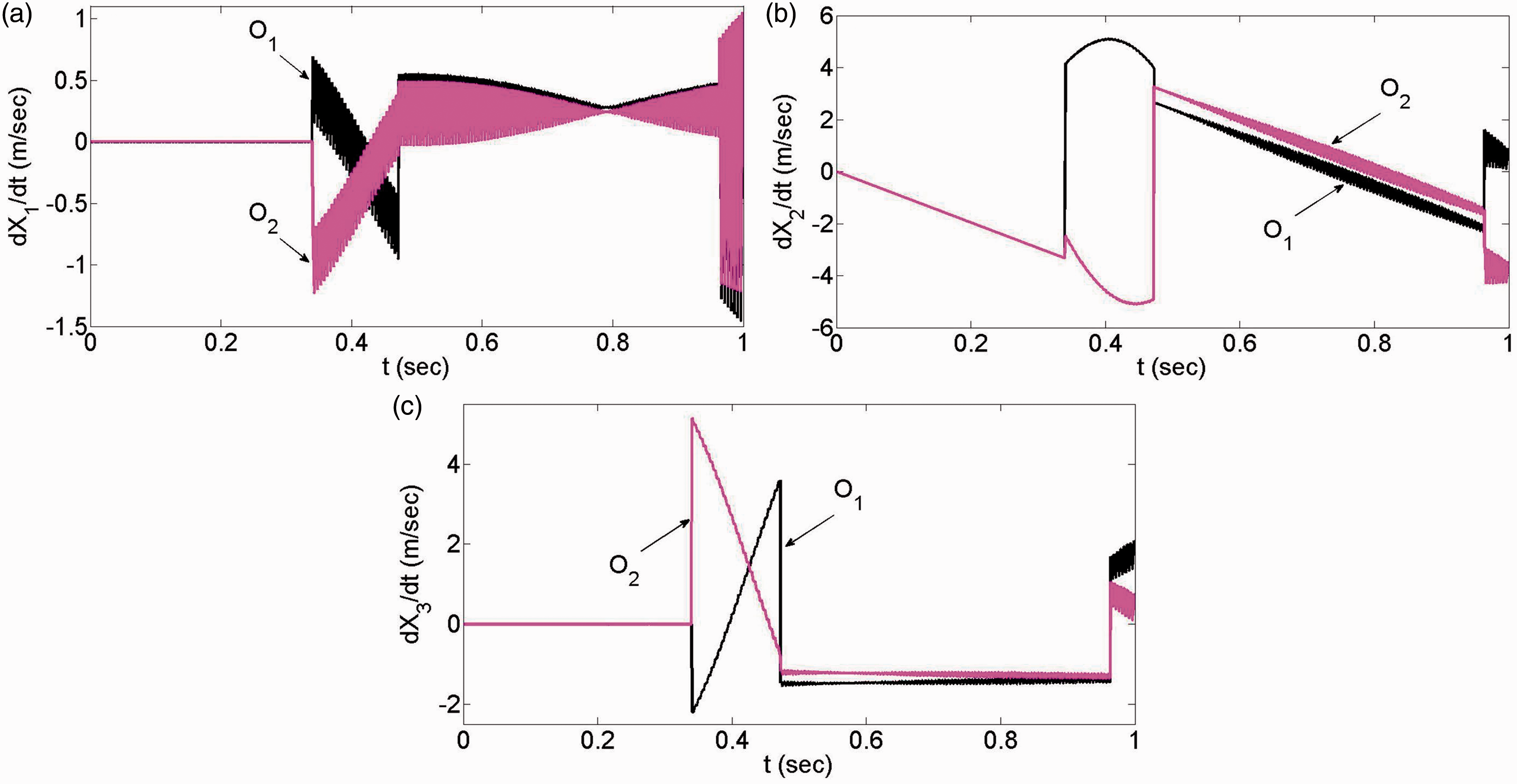
q - 1 = q 0 = q 1 | t = 0 = \frac{π}{6} rad; δ 11 | t = 0 = 0; X 1 | t = 0 = 0.0625; X 2 | t = 0 = - 0.375; X 3 | t = 0 = - 0.3248 q \cdot - 1 = q \cdot 0 = q \cdot 1 | t = 0 = 0 \frac{rad}{s}; δ \cdot 11 | t = 0 = 0 \frac{1}{s}; X \cdot 1 = X \cdot 2 = X \cdot 3 | t = 0 = 0 \frac{m}{s}

The time responses of the system as well as the configurations of this single flying link at the impact moments are depicted in Figures 23–30.

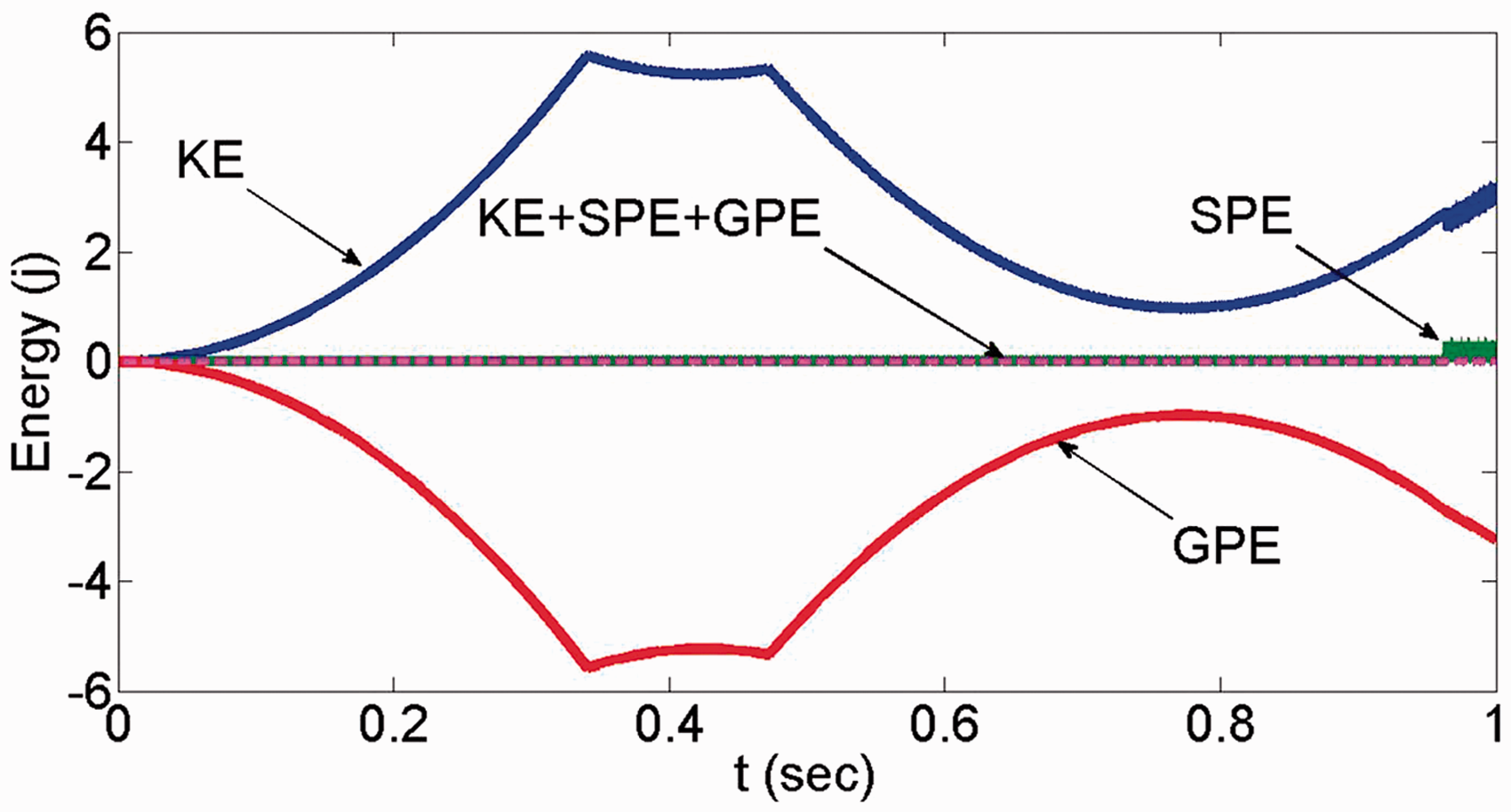
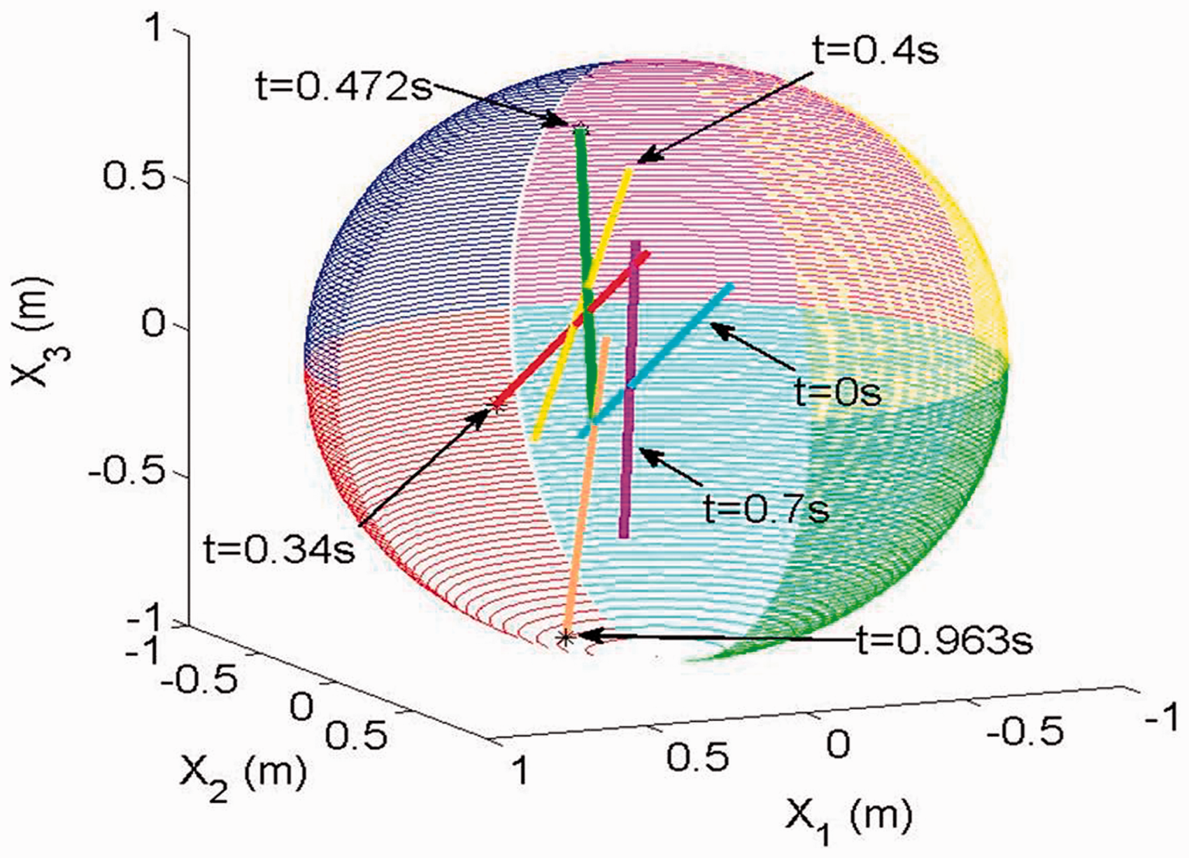
Figure 30 displays the collisions of the first joint, i.e., O₁, with the red section of the sphere at $t = 0.34 s$ and $t = 0.963 s$ . These impact times are shown in this figure by symbol ★. Similarly, it is observed that O₂ touches the purple section of the sphere at $t = 0.472 s$ . This impact is marked by symbol ⋆ in Figure 30. As expected, at these three impact times during the simulation, the quasi-velocities of the link show rapid changes in their values, as illustrated in Figures 24, 26 and 28. The initial configuration of the link indicates that its centroid is located on the reference plane at $X 2 = 0 m$ , where the gravitational potential energy is assumed to be zero. So, since the system is conservative, it is reasonable for the sum of the kinetic and potential energies of the link to remain constant during the simulation (Figure 29). The stability of system responses is highly dependent on the step size. Therefore, besides solving these differential-algebraic equations by employing different ODE solvers and the EVENTS function available in the MATLAB software, a computer program based on various orders of Runge-Kutta method was also used. In this method, the orders were increased until no significant error was observed.

5. Conclusions

In this paper, a recursive approach was presented for the dynamic modeling of oblique impact involving multi-flexible-link robotic manipulators. The contributions of this work can be summarized as follows:

The proposed method can model a chain of n real flexible links which are confined within a closed environment with curved walls. To our knowledge, this is the first time the effect of impulsive motion due to the collision of a multi-flexible-link system with curved surrounding surfaces has been recursively incorporated into the finite motion.

The G-A methodology, which requires fewer total and partial differentiations compared to the Lagrangian formulation, has been applied to generate the governing equations in the flight phase. In fact, even a little reduction in the number of mathematical operations could significantly improve the efficiency of the applied algorithm. Consequently, a less costly computational procedure can be used to satisfactorily simulate the same model.

Deriving the motion equations for an n-elastic-link robotic manipulator by hand is likely to produce error. So, a recursive algorithm based on 4 × 4 transformation matrices has been developed to automatically derive the governing equations. The main advantage of the motion equations obtained by the 4 × 4 transformation matrices (instead of the 3 × 3 rotational matrices which suffer from lengthy formulations) is the compact forms of the derived symbolic formulations; which are achieved by combining the rotations and translations in the 4 × 4 matrices.

In deriving the equations of motions, the manipulators are not restricted to only planar motions. In fact, two virtual links are added to the n real links of a multi-flexible-link manipulator in order to systematically model the spatial rotations of the system in 3D space.

In deriving the motion equations of this complex robotic system, the manipulators are assumed to be composed of only one flexible chain. So, for future works, the procedure used in this paper can be extended to model tree-like robotic systems with more flexible chains. Moreover, the effects of oblique impact on closed flexible chains can be recursively considered in future studies.

Footnotes

Declaration of Conflicting Interests

The author(s) declared no potential conflicts of interest with respect to the research, authorship, and/or publication of this article.

Funding

The author(s) received no financial support for the research, authorship, and/or publication of this article.

Appendix

References

Boghiu

Marghitu

(1998) The control of an impacting flexible link using fuzzy logic strategy. Journal of Vibration and Control 4: 325–341.

Book

(1984) Recursive Lagrangian Dynamics of Flexible Manipulator Arms. The International Journal of Robotics Research 3: 87–101.

Boyer

Khalil

(1998) An efficient calculation of flexible manipulator inverse dynamics. The International Journal of Robotics Research 17: 282–293.

Briot

Khalil

(2013) Recursive and symbolic calculation of the elastodynamic model of flexible parallel robots. The International Journal of Robotics Research 33: 469–483.

Chang

Peng

(2007) Impulsive motion of multibody systems. Multibody System Dynamics 17: 47–70.

Chapnik

Heppler

Aplevich

(1991) Modeling impact on a one-link flexible robotic arm. IEEE Transaction on Robotics and Automation 7: 479–488.

Chevallereau

Westervelt

Grizzle

(2005) Asymptotically Stable Running for a Five-Link, Four-Actuator, Planar Bipedal Robot. The International Journal of Robotics Research 24: 431–464.

Goswami

Thuilot

Espiau

(1998) A Study of the Passive Gait of a Compass-Like Biped Robot: Symmetry and Chaos. The International Journal of Robotics Research 17: 1282–1301.

Heppler

Kariz

(2000) A controller for an impacted single flexible link. Journal of Vibration and Control 6: 407–428.

10.

Hurmuzlu

Marghitu

(1994) Rigid body collision of planar kinematic chain with multiple contact points. The International Journal of Robotics Research 13: 82–92.

11.

Izumi

Hitaka

(1997) Hitting from Any Direction in 3-D Space by a Robot with a Flexible Link Hammer. IEEE Transactions on Robotics and Automation 13: 296–301.

12.

Khulief

(2000) Spatial Formulation of Elastic Multibody Systems with Impulsive Constraints. Multibody System Dynamics 4: 383–406.

13.

Khulief

(2012) Modeling of impacts in multibody systems: An overview. Journal of Computational and Nonlinear Dynamics 8: 1–15.

14.

Khulief

Shabana

(1987) A continuous force model for the impact analysis of flexible multibody systems. Mechanism and Machine Theory 22: 213–224.

15.

Korayem

Shafei

(2013) Application of recursive Gibbs–Appell formulation in deriving the equations of motion of N-viscoelastic robotic manipulators in 3D space using Timoshenko Beam Theory. Acta Astronautic 83: 273–294.

16.

Korayem

Shafei

(2015a) A new approach for dynamic modeling of n-viscoelastic-link robotic manipulators mounted on a mobile base. Nonlinear Dynamics 79: 2767–2786.

17.

Korayem

Shafei

(2015b) Motion equation of nonholonomic wheeled mobile robotic manipulator with revolute–prismatic joints using recursive Gibbs–Appell formulation. Applied Mathematical Modeling 39: 1701–1716.

18.

Kövecses

Cleghorn

(2003) Finite and impulsive motion of constrained mechanical systems via Jourdain’s principle: discrete and hybrid parameter models. International Journal of Non-Linear Mechanics 38: 935–956.

19.

Krauss

(2012) Computationally efficient modeling of flexible robots using the transfer matrix method. Journal of Vibration and Control 18: 596–608.

20.

Liu

(2007) Impact dynamic and control of a flexible dual-arm space robot capturing an object. Applied Mathematics and Computation 185: 1149–1159.

21.

Lugris

Naya

Gonzalez

Cuadrado

(2007) Performance and application criteria of two fast formulations for flexible multibody dynamics. Mechanics Based Design of Structures and Machines 35: 381–404.

22.

Modarres Najafabadi

Kövecses

Angeles

(2007) Energy analysis and decoupling in three-dimensional impacts of multibody systems. ASME Journal of Applied Mechanics 74: 845–851.

23.

Mohan

Saha

(2009) A recursive, numerically stable, and efficient simulation algorithm for serial robots with flexible links. Multibody System Dynamics 21: 1–35.

24.

Seidi

Hajiaghamemar

Caccese

(2015) Evaluation of effective mass during head impact due to standing falls. International Journal of Crashworthiness 20: 134–141.

25.

Shabana

(1997) Flexible multibody dynamics: Review of past and recent developments. Multibody System Dynamics 1: 189–222.

26.

Shabana

Hwang

(1993) Dynamic coupling between the joint and elastic coordinates in flexible mechanism systems. The International Journal of Robotics Research 12: 299–306.

27.

Tlalolini

Aoustin

Chevallereau

(2010) Design of a walking cyclic gait with single support phases and impacts for the locomotor system of a thirteen-link 3D biped using the parametric optimization. Multibody System Dynamics 23: 33–56.

28.

Tornambè

(1999) Modeling and control of impact in mechanical systems: Theory and experimental results. IEEE Transactions on Automatic Control 44: 294–309.

29.

Yigit

(1995) On the Use of an Elastic-Plastic Contact Law for the Impact of a Single Flexible Link. Journal of Dynamic Systems, Measurement, and Control 117: 527–533.

30.

Wasfy

Noor

(2003) Computational strategies for flexible multibody systems. Applied Mechanics Reviews 56: 553–613.

31.

Zhang

Angeles

(2005) Impact dynamics of flexible-joint robots. Computer and Structures 83: 25–33.