
Abstract
In this work, a boundary layer control scheme for one-dimensional wave propagation problems is presented that provides reflection-less absorption of incident waves in numerical simulations. The desired absorption properties are formulated as an optimization problem. By using the dispersion relation to predict the unbounded wave propagation as a reference trajectory, a constant-gain state-feedback boundary layer controller is found. Since no additional auxiliary variables are introduced, this approach is highly computationally efficient, making it suitable for simulations under real-time requirements. The performance of the boundary layer controller is first evaluated and demonstrated on the scalar wave equation (vibrating string), for which reference absorbing boundary conditions are well established. Afterward, the moving Euler–Bernoulli beam under axial tension is considered, for which a good absorbing performance is achieved.
Keywords
1. Introduction
One-dimensional wave propagation problems, described by partial differential equations are extensively used in practical engineering applications, for example, when modeling the vibrations of beams, railway tracks (Vostroukhov and Metrikine, 2003), overhead lines (Ritzberger et al., 2015), or bandsaws and conveyor belts (Tang et al., 2015). Approximate solutions can be obtained by applying numerical techniques, such as the finite-difference method. Thereby, the domain is truncated and suitable boundary conditions must be introduced. By applying absorbing boundary conditions, ideally waves are attenuated without generating reflections at the boundary; thus, the solution of the truncated domain approximates the unbounded wave solution (see Figure 1).
When the wave is totally absorbed at the boundary, the solution inside the computational domain approximates the free-wave solution.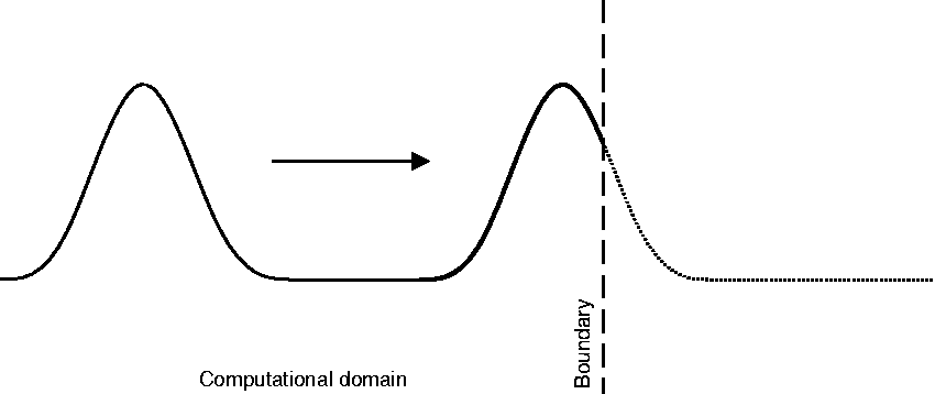
In early works (Engquist and Majda, 1977; Higdon, 1987), absorbing boundary conditions were derived under the assumption of constant wave propagation speed. These localized absorbing boundary conditions are easy to implement, but if dispersion is present, i.e. the wave propagation speed depends on the spatial frequency, the absorbing performance is severely impaired. Another type of absorbing boundary condition, introduced by Berenger (1994), is the perfectly matched layer (PML). Thereby, the computational domain is surrounded by a layer of finite thickness in which waves are efficiently attenuated. Chew and Weedon (1994) interpreted the PML approach in terms of using complex coordinate stretching, and extended its application to dispersive wave problems.
Although good performance can be achieved with the PML, its implementation relies on problem-specific transformations of the partial differential equation. Thereby, depending on the order of the spatial derivatives, the solution field is split or, in the case of high-order spatial derivatives, several auxiliary partial differential equation are introduced (Hesthaven, 1998). Doing this can lead to long-term instability (Abarbanel et al., 2002) and drastically increases the computational effort.
In this work, the construction of an absorbing boundary layer is perceived as an optimal boundary control problem. The main contribution is a novel method of combining a dispersion-relation-based prediction of the unbounded wave solution, which serves as a desired reference trajectory, and an associated optimal control problem, closely related to the model predictive control theory, with inputs distributed across the boundary layer. Effectively, this method realizes an impedance controller aiming at emulating the physical properties of the unbounded domain. By appropriately introducing the unbounded wave prediction in terms of linear operations, it is shown that online optimization of the control inputs, typical in model predictive control, is avoided and a time-invariant state-feedback controller is obtained.
The proposed control scheme provides the advantage that the partial differential equations under consideration do not need to undergo problem-specific transformations, and therefore no auxiliary fields are introduced. A simple state-feedback controller achieves the desired PML-like behavior instead, making this approach highly computationally efficient and suitable for real-time applications. Since the control design is carried out directly on the discretized system, dispersion due to discretization is inherently considered and does not decrease the absorbing performance. The controller design can be highly automated and is therefore easily adapted to different kinds of linear one-dimensional wave propagation problem.
The absorbing capabilities will be first investigated for the one-dimensional scalar wave equation, since absorbing boundary conditions are well established for this type of problem and the performance in comparison with these reference absorbing boundary conditions can be investigated through numerical simulations. Thereafter, the proposed control scheme is applied to the moving Euler–Bernoulli beam under axial load, for which, to the authors’ best knowledge, alternative absorbing boundary conditions have not yet been devised. In comparison, alternative absorbing boundary conditions for the simplified nonmoving Euler–Bernoulli beam without axial load, such as the classic PML approach derived by Arbabi and Farzanian (2014) or the procedure proposed by Montseny (2011), become highly problem-specific and several auxiliary partial differential equations or additional dynamic state variables are introduced.
2. Fundamentals
In this work, dynamic linear one-dimensional partial differential equations of the form

2.1. Finite-difference approximation
To obtain an approximate solution of a partial differential equation, various numerical techniques can be applied. One possibility is the finite-difference time-domain method. The partial derivatives in equation (1) are thereby approximated by their corresponding central finite differences (Strikwerda, 2007).
By defining a fixed step size Δt and Δx for time and space, the solution is only available at discrete points


2.2. Boundary conditions
Since it is assumed that, owing to the controlled damping layer, all waves are sufficiently attenuated, simple clamped boundary conditions

2.3. Dispersion relation
For a linear wave-like partial differential equation with constant coefficients, the harmonic wave (as in Hagedorn and DasGupta, 2007)


3. Main results
In this section, the objective function that evaluates the absorbing performance of a controller and serves as the base of the optimization problem will be discussed. Afterward, two methods are presented that facilitate a useful solution: an analytical treatment of the optimization problem and numeric optimization using a genetic algorithm.
3.1. Optimization problem formulation
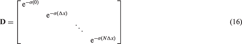
The state-space system (2) is to be controlled so that, based on the idea of complex coordinate stretching (see Appendix 1 for details), an exponential decay is added to the harmonic wave solution (5)

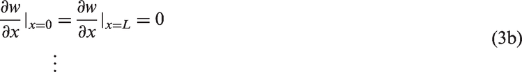
With additional control inputs at the nodes in the damping layer (see Figure 2), the state-space system is extended to
Resulting control scheme for the analytic optimization, Nc = 6. Red nodes are pinned, realizing a clamped boundary condition. The complete state vector is used.


3.2. Analytic solution of the optimization problem
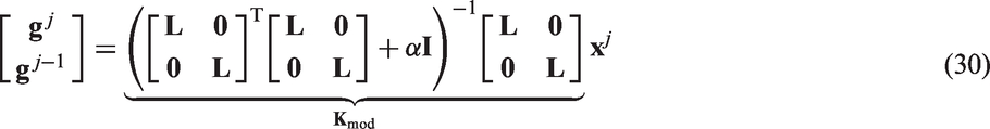
By applying a modal decomposition to the displacement vector It is assumed that the displacement vector
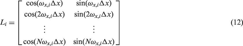
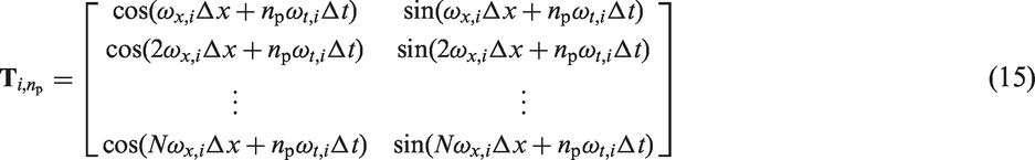
Given Assumption 1, the modal decomposition of the current displacement vector Applying a temporal shift In Lemma 1, it is assumed that the amplitudes of waves traveling in the reverse direction, from the damping layer into the computational domain, is zero. This is a justified assumption as long as there are no additional disturbances exciting the system inside the damping layer and if the desired attenuation of waves is sufficiently large that spurious reflections at the boundaries become negligible. Therefore, only waves traveling from the interior domain into the damping layer are considered in the prediction. Given a system of the form of equation (9), and using Lemma 1, an optimal linear state-feedback control law
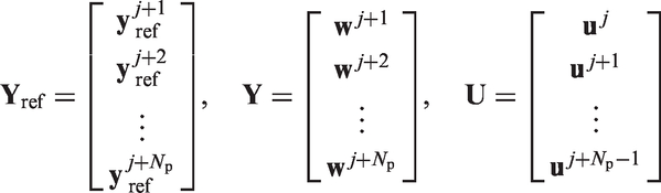
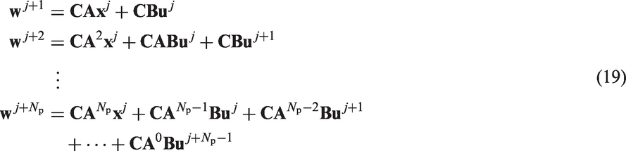
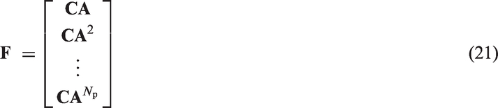
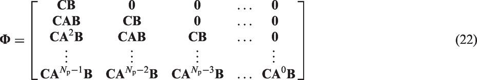
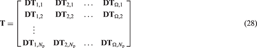
With the extended state-space system (9), the future states based on the current state information are predicted sequentially up to Np time steps
Assumption 1
Lemma 1
Proof
Remark 1
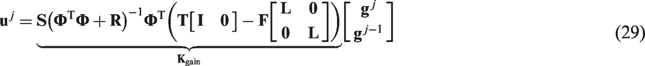
Theorem 1
Proof


The state vector In the control law (equation (17)) proposed in Theorem 1, the complete state vector of the system (9) is used. A schematic representation of the control scheme is shown in Figure 2.Remark 2


3.3. Direct optimization under structural constraints
As an alternative, a direct optimization technique (e.g. genetic algorithm) can be used to optimize the objective function (10). This allows for additional structural assumptions about the controller to be made. An example structure that has proven to be useful, as it offers a good trade-off between absorbing performance and number of parameters to be optimized, is
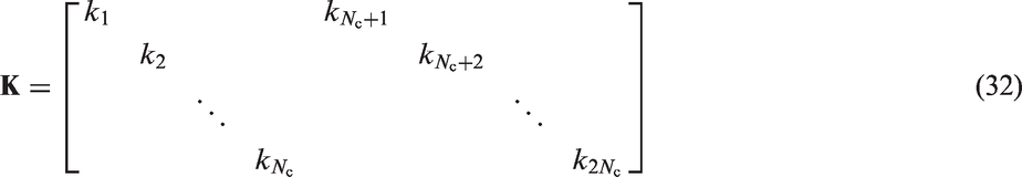

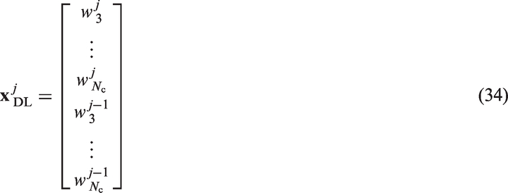
A schematic illustration of the resulting control scheme is depicted in Figure 3. By contrast with the analytic optimization shown in Figure 2, a reduced state vector is fed back into the control gain matrix Schematic damping layer controller obtained by using a genetic algorithm, Nc = 6.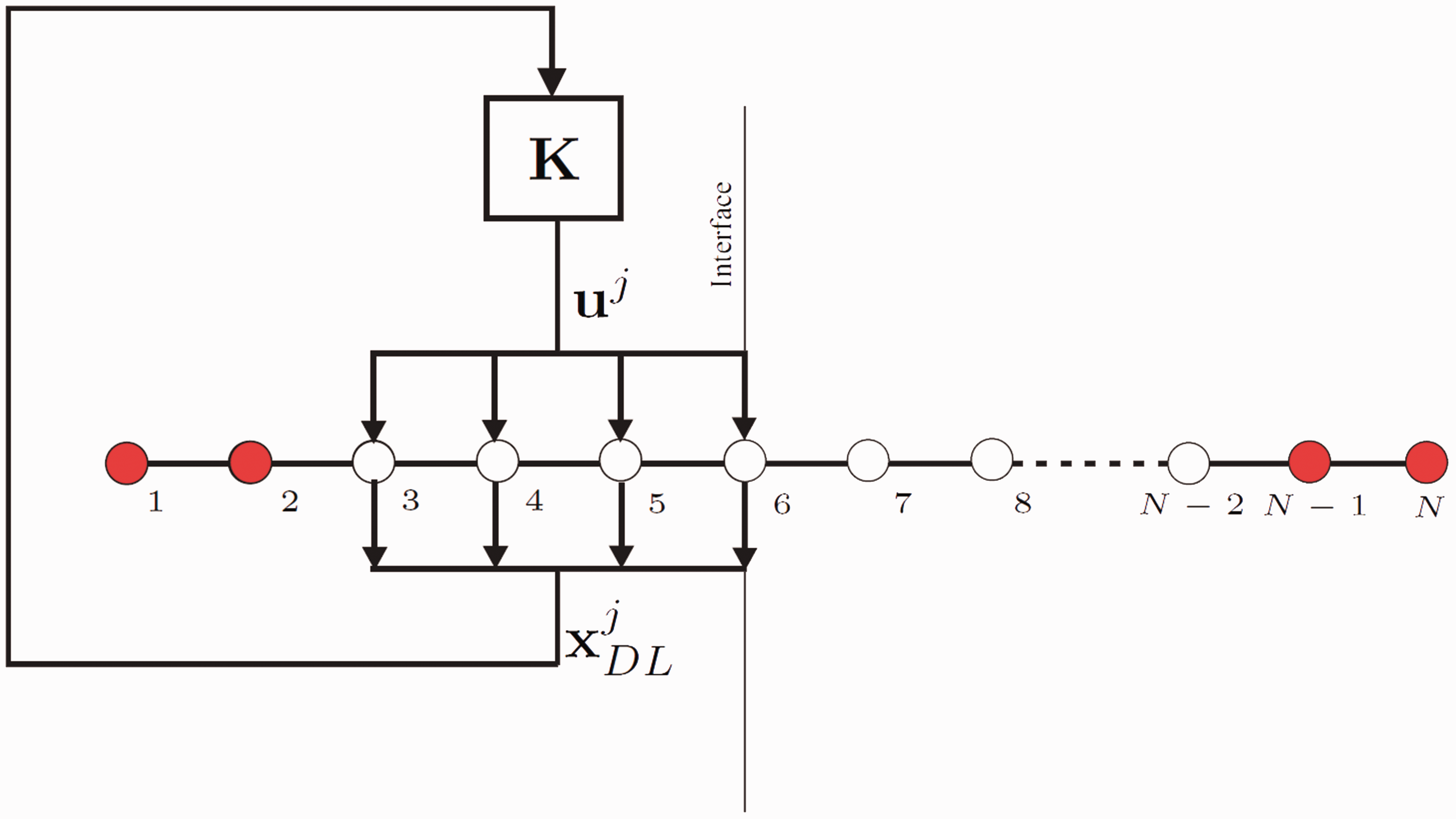
The goal of the genetic optimization is to find the set of parameters of the control gain matrix of equation (32). To achieve this goal, an initial set of solution candidates is created. In each iteration, these candidates are manipulated by selection, mutation, and recombination, and a new generation is formed. Ideally, the objective function is thereby minimized and the population converges after several generations. Owing to its random nature, the final generation differs for each optimization run and convergence to a useful solution is not guaranteed. By contrast, the analytic optimization approach is reproducible in the sense that with the same initial problem setup the same optimal controller is found. The advantage of using the genetic algorithm lies in the fact that the optimization framework can be set up fairly quickly, assuming that a suitable optimization software (e.g. MATLAB Optimization Toolbox™) is available. Furthermore, the structure of the controller can be assessed directly; this can be advantageous under certain circumstances, for example, if a sparse structure is desired to further accelerate the computation (at the cost of absorbing performance) or a certain physical structure, such as an elastic bedding, is to be used.
4. Numerical simulation
At first, the scalar one-dimensional wave equation will be considered, for which absorbing boundary conditions are well established.
Finally, the presented method will be applied to the moving Euler–Bernoulli beam under axial tension, for which no alternative absorbing boundary technique is available.
4.1. Scalar wave equation
The problem considered in this section is the one-dimensional wave equation given by

4.1.1. Dispersion relation
Inserting the harmonic wave solution (4) into equation (35) yields the continuous dispersion relation
Phase velocities for different Courant numbers λ.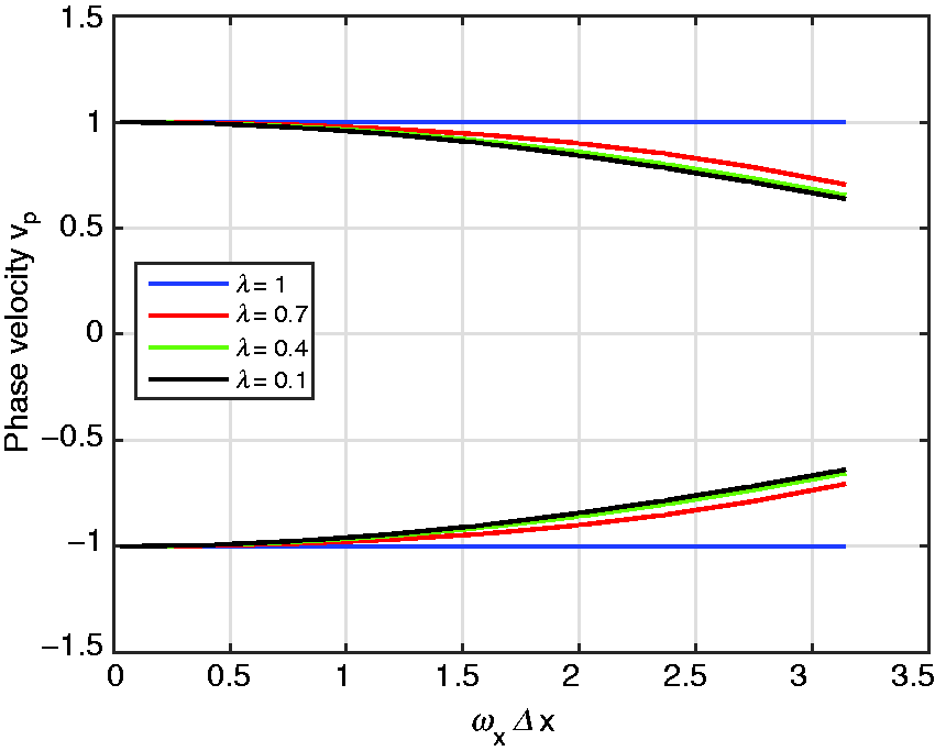


4.1.2. Numerical setup and reference systems
The domain of interest is defined to have N = 200 nodes and absorption is desired at both boundaries. The nominal wave speed is set to c = 1, the time step size to Δt = 0.1 and the spatial step size to Δx = 1. Therefore, the Courant number is λ = 0.1, which causes significant numerical dispersion. To compare the performance of the controlled damping layer, the following reference systems are used:
An enlarged reference system with Dirichlet boundary conditions and Nref = 20N spatial nodes. The reflection error is assessed with respect to this enlarged reference system, since spurious reflections do not reach the domain of interest during the simulation. A reference system with first-order Engquist–Majda absorbing boundary conditions (Engquist and Majda, 1977), which are perfectly absorbing for the one-dimensional wave equation if λ = 1. Since λ = 0.1, a decrease of the absorbing performance for high spatial frequency waves is expected. An unsplit PML formulation is obtained through complex coordinate stretching, which is described by Grote and Sim (2010), and uses a space-time staggered grid with explicit time stepping. Here, however, the same simple collocated grid scheme as in the other reference systems was used. As a result, numerical (long-term) instability was observed. As the unstable dynamics are only relevant at time scales of one order of magnitude greater than the desired simulation time, the comparison is deemed valid here.
4.1.3. Damping layer controller
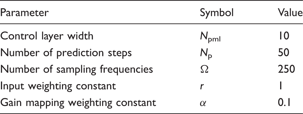
Optimization parameters.
The damping profile used in equation (16) is chosen as a quadratic function of the form
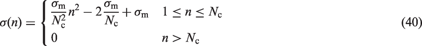
A useful property of the resulting control matrix is that the discrete system for which the optimization is carried out does not need to be of the same size as the system on which the controller is later applied. In this case, the system for the optimization consists of Nopt = 100 nodes. When applied to the system with N = 200 nodes only the states present at the optimization are fed back to the controller. Since the dispersion relation is symmetric for the scalar wave equation, the resulting controller can be applied on both boundaries. However, the elements of the controller have to be rearranged to be consistent with the node order of the displacement vector for the opposite boundary.
4.1.4. Simulation results for one-dimensional wave equation
The initial conditions for all system were set to be a pulse of the form
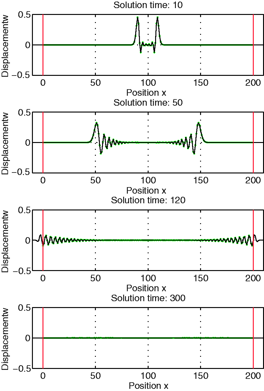
Wave equation with initial pulse. Comparison of simulation results between controlled damping layer and enlarged reference system.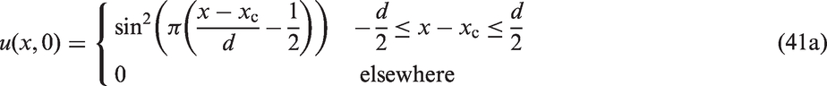

4.1.5. Error evaluation
To quantify the error in comparison with the enlarged reference system, the following measure is used
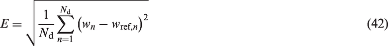
Figure 6 shows the error over time for the controlled damping layer in comparison with the Engquist–Majda absorbing boundary condition, the PML obtained through complex coordinate stretching, and the clamped boundary. Since the finite-difference time-domain method used to obtain a numerical solution is explicit, the results for the clamped boundary, the absorbing boundary condition, and the PML do not deviate from the reference solution significantly until the wave front impacts the boundary (t ≈ 90 s). For the controlled damping layer, a deviation can be observed much earlier. This is because the inputs for the damping layer controller are the displacements of nodes that reach far into the computational domain. Therefore, slight control action occurs before the wave package reaches the interface. The majority of the wave package has left the computational domain at t ≈ 300 s. The Engquist–Majda absorbing boundary conditions suffer from the numerical dispersion caused by the Courant number λ = 0.1 and produce significant reflections, especially in the high spatial frequency range. The PML obtained through complex coordinate stretching shows a good performance at the impact of the wave package but, as mentioned earlier, the simple discretization scheme has a negative effect on long-term stability and the error starts to increase with time. The controlled damping layer, although deviating sooner from the reference solution, shows a good absorbing performance by having a smaller reflection error than the Engquist–Majda absorbing boundary condition and the PML.
Error evaluated for the different absorbing boundary methods over time for the initial pulse simulation. ABC: absorbing boundary conditions; PML: perfectly matched layer.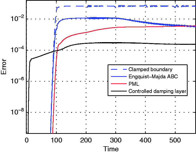
4.2. Moving Euler–Bernoulli beam
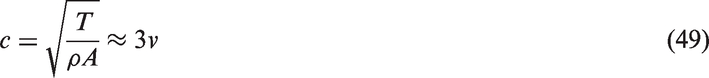
In this test case, the controlled damping layer will be applied on the moving Euler–Bernoulli beam equation (Wickert and Mote, 1990)

4.2.1. Deriving the state-space system representation
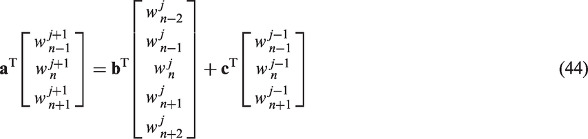
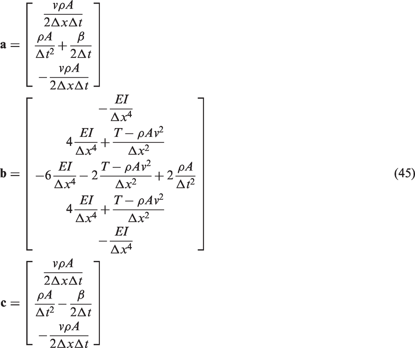
After discretization, an algebraic equation for each grid point is obtained that describes the dependency to its surrounding nodes in space and time


4.2.2. Dispersion relation
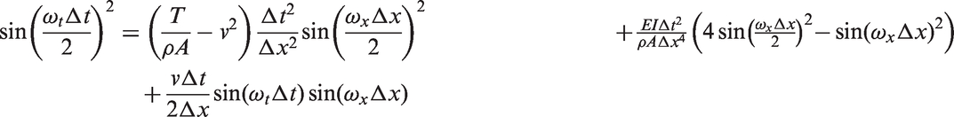
As with the numeric example of the scalar wave equation above, inserting equation (5) into equation (44) yields the so-called discrete dispersion. After simplification, the following implicit function for the moving Euler–Bernoulli beam is obtained
4.2.3. Simulation results for the moving Euler–Bernoulli beam
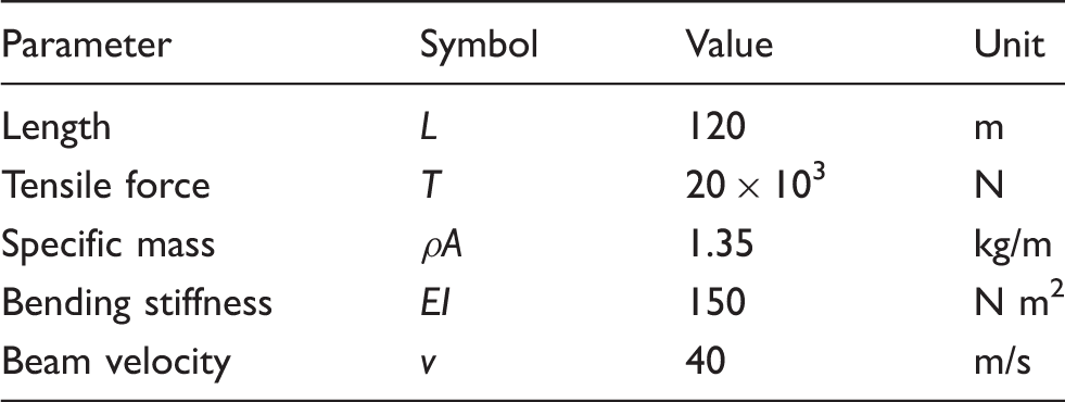
System parameters.
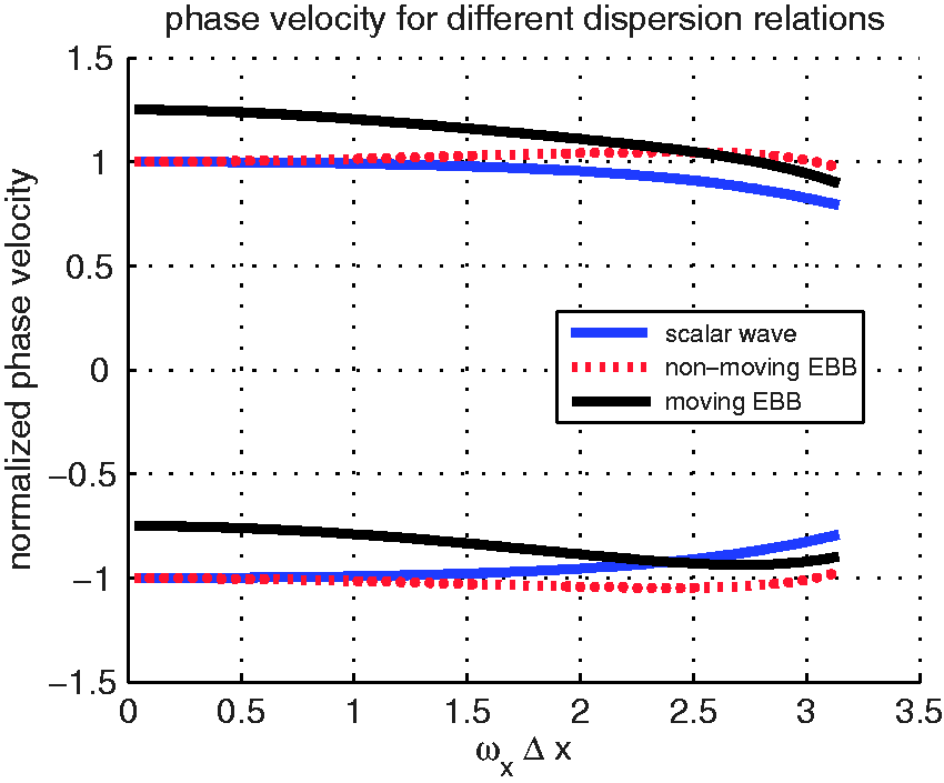
Normalized phase velocity plot for the scalar wave (blue), nonmoving Euler–Bernoulli beam (EBB) (red) and moving Euler–Bernoulli beam (black).
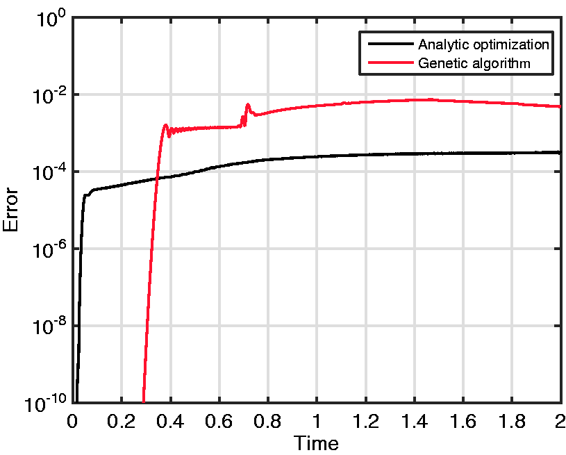
Figure 8 gives a visual comparison between the system with controlled damping layer and an enlarged reference system. The direction-dependent propagation speed of waves is evident. A good agreement with no visible reflections at the interface can be observed. In Figure 9, the reflection errors according to equation (42) for the controlled damping layer obtained through analytic optimization and the control layer using a genetic algorithm are compared. The optimization parameters, namely the prediction horizon and the number of sampled spatial frequencies, are chosen to be equal. The analytic solution achieves a higher absorption performance than the structured genetic algorithm solution. The simple diagonal substructure (equation (32)) used in this example gives a reasonable trade-off between performance and robustness of the optimization. More complex structures can lead to better performance, as there are more degrees of freedom. However, with an increasing number of parameters to be optimized, convergence to a practical solution is more unlikely and time-consuming. Since for the numerically optimized controlled damping layer only the states inside the layer itself are fed into the gain matrix, a significant deviation from the reference system occurs when the wave package passes over the interface. By contrast, only a small deviation for the analytically optimized control layer is evident from the start.
Moving Euler–Bernoulli beam with initial pulse. Comparison of the simulation results between controlled damping layer (black) and the enlarged reference system (green). Error with respect to the enlarged reference system for the controlled damping layer obtained through analytic optimization and genetic algorithm.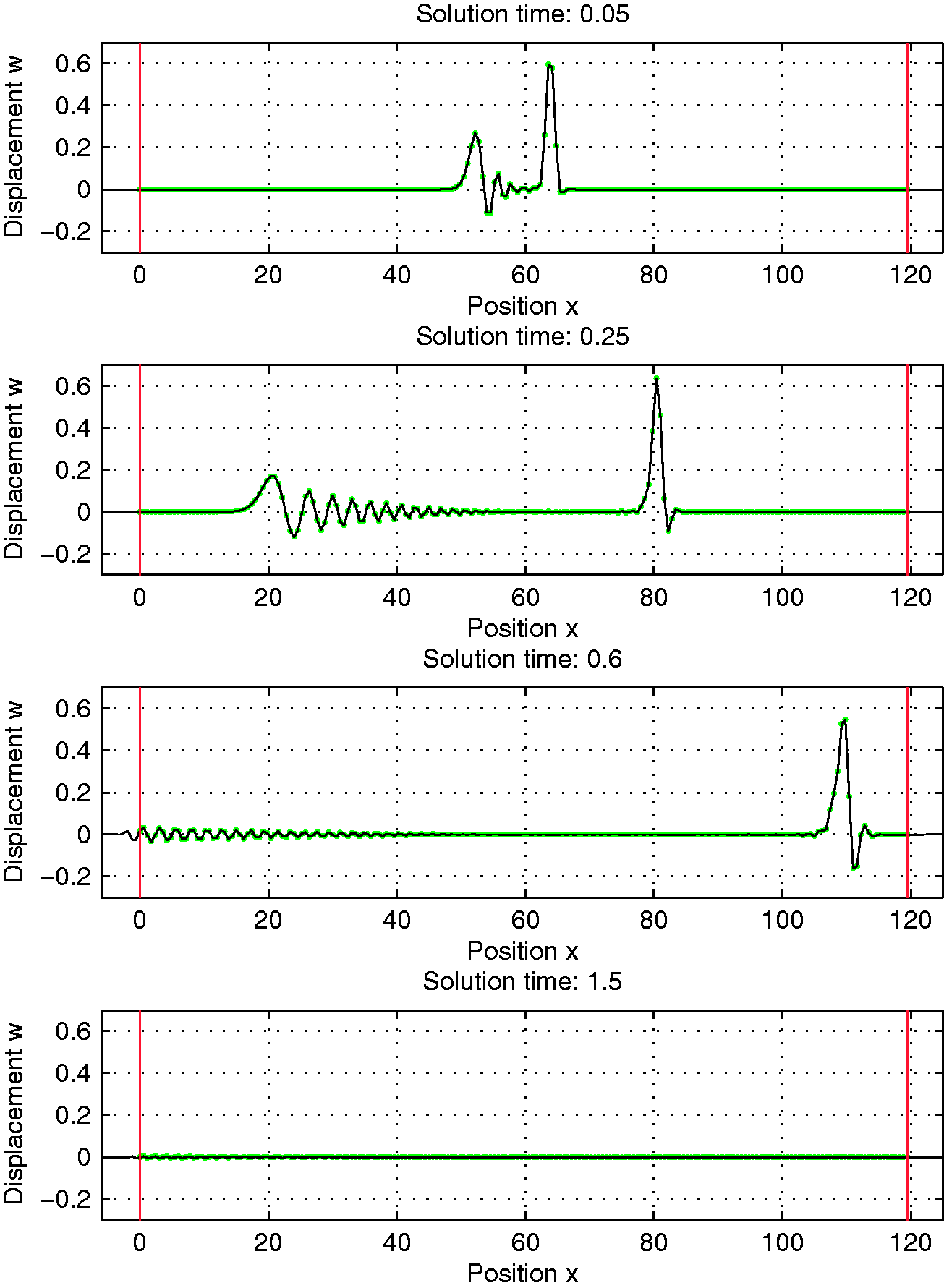
5. Conclusions
In this work, the construction of absorbing boundary conditions is interpreted as an optimal boundary control problem and solved using modal decomposition and modal prediction of the unbounded solution. As a result, a time-invariant state-feedback control law is obtained that emulates the absorbing properties of a PML. The scalar wave equation is investigated, for which reference absorbing boundary conditions are well known, and the effectiveness of the proposed method in comparison with standard absorbing boundary conditions is demonstrated in simulations. Additionally, extensive transformations of the original problem and the introduction of auxiliary partial differential equations are avoided. The same method is then applied to the moving Euler–Bernoulli beam equation under axial tension, for which alternative absorbing boundary conditions are not available. The proposed optimal control method again achieves high absorbing performance and computational efficiency. Since the control design uses the discretized system, numerical dispersion due to discretization is inherently considered and does not decrease the performance, as is the case for absorbing boundary conditions, which are designed in continuous time. The ease of adaptability, design, and low computational effort, combined with good absorbing performance, makes this approach highly valuable for time-critical simulations of unbounded one-dimensional wave propagation problems.
Footnotes
Declaration of Conflicting Interests
The author(s) declared no potential conflicts of interest with respect to the research, authorship, and/or publication of this article.
Funding
The author(s) received no financial support for the research, authorship, and/or publication of this article.