A novel method for force identification based on filter and FEM

Abstract

Force identification plays a vital role in vibration control and structural health monitoring. Force identification is an inverse problem to determine the excitation load from the responses. In general, the inverse problem has strong ill-posedness and ill-condition, especially in the case of low signal-to-noise ratio. Singular value decomposition and Tikhonov regularization are widely used for the reconstruction of the input force. Nevertheless, the anti-noise performance and accuracy of the two methods are still unsatisfactory. In this paper, we present a novel method for force identification based on a filter and the finite element method (FEM). The filter is used to suppress the noise of the input signals. FEM is introduced to reduce the discretization error and the regularization parameters are optimized by the genetic algorithm. After the signal is filtered, the characteristics of the signal will be changed. Especially, the initial and the last segments of the input signal will be lost. These changes may make the identified force inaccurate, even more inaccurate than the force identified with no filtering. To deal with this problem, cubic spline interpolation and a nonlinear autoregressive neural network are introduced to repair the input signals. Finally, three numerical examples and experiments are used to verify the superiority of the method.

Keywords

Force identification Tikhonov regularization finite element method genetic algorithm filter

1. Introduction

With the development of simulation technology, it now plays an important role in scientific research and is widely used in engineering such as vibration control, structural design, and motion analysis. In vibration simulation, the force acting on the mechanical structure is the critical boundary condition and has a great influence on the accuracy of simulation results. However, in many situations, it is difficult or even impossible to use the force transducer, because the transducer may induce changes to the dynamic characteristics of the structure or due to the limitations of the structure. Even if the force can be measured, it usually requires high experimental costs. In contrast, the response of the structure such as displacement, velocity and acceleration can be conveniently measured at a lower cost. The determination of the unknown force from the corresponding response is called force identification, which has been developed for many years (Stevens, 1987; Janssens et al., 2011). However, force identification as an inverse problem suffers from ill-posedness and ill-condition. The solution of force identification is sensitive to the noise of the input; even small disturbances in the input may lead to large deviations in the solution. Many force identification algorithms have been proposed by scholars to solve this problem.

Force identification involves the determination of the location, magnitude, and spatial distribution of the force. Initially, the study of force identification began with the identification of the magnitude of a force whose location was known. The force is reconstructed by multiplying the inverse matrix of the transfer function matrix with the corresponding response. However, this direct method is not applicable in most situations due to the singularity of the transfer function. Jayalakshmi et al. (2018) found that the direct method is highly sensitive to noise and has severe practical limitations. In view of this problem, the Tikhonov regularization based on the variational principle was proposed (Tikhonov, 1963; Tikhonov and Goncharskiĭ, 1987). It can effectively overcome the ill-posedness of the inverse problem by adding a penalty term to the vibration equation. Many force identification algorithms based on Tikhonov regularization have been proposed. Li and Lu (2018) proposed a two-step iterative approach for locating and reconstructing single-point forces acting on structures. The approach can locate the force whose location does not coincide with the nodes of the mesh in a fast, iterative manner. Aucejo and De Smet (2018) presented an original iterated multiplicative regularization based on the iterated Tikhonov regularization. This method takes prior knowledge of the signals into account and does not need to choose the regularization parameters. In addition, he and his collaborators (Aucejo et al., 2019) introduced a novel reconstruction model based on the generalized-α method. This model is unconditionally stable and has second-order accuracy. The concept of adaptive regularization was proposed by Ryzhikov and Biryulina (1998) and it was further described by Ma and Wang (2005). The adaptive regularization is similar to Tikhonov regularization, but more effective in suppressing the fluctuation of results. Regardless of the adaptive regularization or Tikhonov regularization, the selection of regularization parameters is important. There are two strategies for choosing regularization parameters: posterior strategy and prior strategy. In general, the prior strategy is convenient for theoretical analysis, but it is difficult to use in engineering because it may require some prior information which is hard to obtain. In contrast, the posterior strategy does not suffer from this problem. Hence, the posterior strategy is widely used. There are many effective posterior strategies. The Morozov deviation principle is a commonly used posterior strategy. It works well only when the error level of the input is known. Further research on the application of the posterior strategy (Morozov, 1984; Kunisch and Zou, 1998; Wang and Xiao, 2001; Wang, 2003) has been conducted. However, the noise of the measured signal is usually unknown in most cases. In view of this, a lot of research has been done. Golub et al. (1979) introduced a generalized cross-validation (GCV) approach which derived from Allen's PRESS method (Allen, 1971). GCV is a robust and adaptable method. Hanke and Hansen (1993) defined the maximum curvature of the L-curve criterion at the logarithmic scale and used it to select the regularization parameters. Both L-curve criterion and GCV are widely used to determine the regularization parameters (Tveito et al., 2012). The two methods have good adaptability and robustness.

Recently, various methods about force identification and their applications have been studied in depth by scholars. Aucejo (2014) indicated that prior information plays a key role in source identification. De Deus et al. (2012) showed the application of Tikhonov regularization in dynamic elastoplastic problem analysis. On the basis of the modified GCV criterion, an efficient regularized cubic B-spline collocation method was proposed to identify the impact force (Qiao et al., 2015). Qiao et al. (2017) proposed a novel impact force reconstruction method based on the primal-dual interior point method. This method can improve the computational efficiency of the program and the accuracy of the identified impact force. In addition, Qiao and his team have conducted a lot of in-depth research on impact force identification (Qiao et al., 2016a, 2016b, 2019). Mao et al. (2010) developed a force identification approach in time domain for linear systems with Tikhonov regularization. This approach can find a highly precise force identification model within the scope of general computer precision, and it does not cost much computing time. Liu et al. (2015) combined Gegenbauer polynomial expansion theory with a regularization method to identify the dynamic force acting on stochastic structures. A forward model of dynamic load identification was established through the discretized convolution integral of loads and the corresponding unit-pulse response functions of the system. Wang et al. (2015) proposed a novel state space method that was extended to a refined version based on the discretization idea of the finite element method (FEM) to improve the identification accuracy. They investigated the effects of noise, high noise levels, discontinuous loading, and multiple forces reconstruction. Jayalakshmi and Rao (2017) developed a dynamic hybrid adaptive firefly algorithm to effectively identify the system parameters and the input forces. The algorithm maintains a very good balance between intensification and diversification and has better convergence performance. Prawin and Rao (2018) presented an online input force reconstruction algorithm by using dynamic principal component analysis. The force reconstruction algorithm has no physical modeling errors and is less sensitive to noise. In addition, they also presented an optimal sensor placement algorithm to place limited sensors at dynamically sensitive spatial locations.

In this paper, a novel method is developed to identify the input force–time history acting on the structure and examples are used to verify the merits of the method. In this method, filters and a nonlinear autoregressive (NAR) neural network are used to reduce the noise of the input, the FEM is used to reduce the discretization error, and the genetic algorithm (GA) is used to obtain the optimal regularization parameters. This method is a combination of filters, FEM, and GA, called FFGM for short. In Section 2, the basic theory of FFGM is described. In Section 3, the process of FFGM is described in detail. In Section 4, three numerical examples are used to verify the superiority of FFGM. Experiments are conducted to study the performance of FFGM in Section 5. Finally, conclusions are summarized in Section 6.

2. Basic theory

In time domain, force can be expressed as $F (t)$ . As shown in the following equation (1), $F (t)$ can be expressed as the sum of a series of Dirac functions:

F (t) = \int_{0}^{t} F (τ) δ (t - τ) d τ

(1)

where

F (τ)

is the magnitude of the force when the time is τ and δ is the unit impact force.

While the $F (t)$ is applied to a system, the response of the system can be expressed as

R (t) = \int_{0}^{t} F (τ) h (t - τ) d τ

(2)

where

R (t)

denotes the response of the measurement point and

h (t)

is the unit pulse response from the measurement point to the excitation point.

By discretizing equation (2), the following equation can be obtained:

[\begin{matrix} r_{1} \\ r_{2} \\ : \\ r_{m} \end{matrix}] = [\begin{matrix} \begin{matrix} h_{1} Δ t \\ h_{2} Δ t \end{matrix} & \begin{matrix} 0 \\ h_{1} Δ t \end{matrix} & \begin{matrix} \begin{matrix} \dots & 0 \end{matrix} \\ \begin{matrix} \dots & 0 \end{matrix} \end{matrix} \\ : & : & : \\ h_{m} Δ t & h_{m - 1} Δ t & \begin{matrix} \dots & h_{1} Δ t \end{matrix} \end{matrix}] [\begin{matrix} F_{0} \\ F_{1} \\ \begin{matrix} : \\ F_{m - 1} \end{matrix} \end{matrix}]

(3)

where

Δ t

denotes the discrete time interval,

r_{i}

is the response of the measurement point at the ith

Δ t

h_{i}

is the unit pulse response of the measurement point at the ith

Δ t

, and

F_{i}

is the magnitude of exciting force at the ith

Δ t

. In many situations, there is noise in

r_{i}

and

h_{i}

. Therefore, equation (3) can be rewritten as

R_{δ} = H_{δ} F + ɛ

(4)

where

R_{δ}

is the response vector with noise,

H_{δ}

is the unit pulse response matrix with noise, and ɛ is the error vector. According to Tikhonov regularization, the force

F

can be obtained by the following equation:

F = \arg min J (F)

(5)

with

J (F) = ‖ R_{δ} - H_{δ} F ‖ + α F^{T} Φ F

(6)

where

α F^{T} Φ F

is the penalty,

Φ

is a positive definite matrix, and α is the regularization parameter. The following equation can be obtained by solving equation (5):

F = (H^{T} H + α Φ)^{- 1} H^{T} R

(7)

When $Φ$ is an identity matrix, equation (7) is the Tikhonov regularization form. The selection of α is critical in equation (7). The solution will be too smooth to be accuracy when α is too large. On the contrary, the stability of the solution will be too poor when α is too small. For solving this problem, the GCV criterion is adopted to obtain the regularization parameter α. The derivation of the GCV criterion is expressed as follows:

H = US V^{T}

(8)

H_{h} = WS U^{T}

(9)

R_{h} = W U^{T} R

(10)

where

W

denotes the unitary matrix. The jkth entry

[W]_{jk}

W

is shown as follows:

[W]_{jk} = \frac{1}{\sqrt{m}} e^{2 π i (jk / m)}

(11)

According to equations (8)–(11), the expression of the GCV criterion is shown as

V (α) = \frac{‖ [Φ - G (α)] R_{h} ‖ 2}{Tr [Φ - G (α)] 2}

(12)

where α, which minimizes

V (α)

, is the optimal regularization parameter in the GCV criterion.

3. The details of FFGM

Compared with Tikhonov regularization, there are three improvements in FFGM. First, GA is used to calculate the optimal regularization parameter. Second, the recursive Gaussian filter is used to reduce the Gaussian noise of the input. Third, the force is discretized by FEM to reduce the discretization error. Each improvement will be described in detail below.

3.1. Obtain the optimal regularization parameters by GA

For finding the minimum value of $V (α)$ accurately, GA is used to optimize the regularization parameter α. Before generating the chromosome, α is converted to x according to

α = 10^{x}

(13)

where x is encoded as a chromosome in GA.

The population size is 25, the maximum genetic algebra is 20, the length of chromosome is 20, the generation gap is 0.95, the chromosome crossover probability is 0.7, and the chromosome variation probability is 0.01.

3.2. Reduce the noise by using recursive Gaussian filter

In general, there is noise in the input measured. For different types of noise, we can use different filters to suppress noise. There is usually Gaussian white noise in the signals, so the recursive Gaussian filter is used to suppress it. However, the initial and the last segments of the input signal would be lost due to the influence of the recursive Gaussian filter. In Figure 1, an example shows the comparison between unfiltered and filtered signals. Cubic spline interpolation is used to get the lost initial segments of the signal and the NAR network is used to predict the lost last segments of the signal. The NAR network is a dynamical neural structure that is commonly used for modeling nonlinear dynamic systems. The NAR network can be efficiently applied to long-term prediction of univariate time series (Menezes and Barreto, 2008). The NAR network is easy to use and has good robustness.

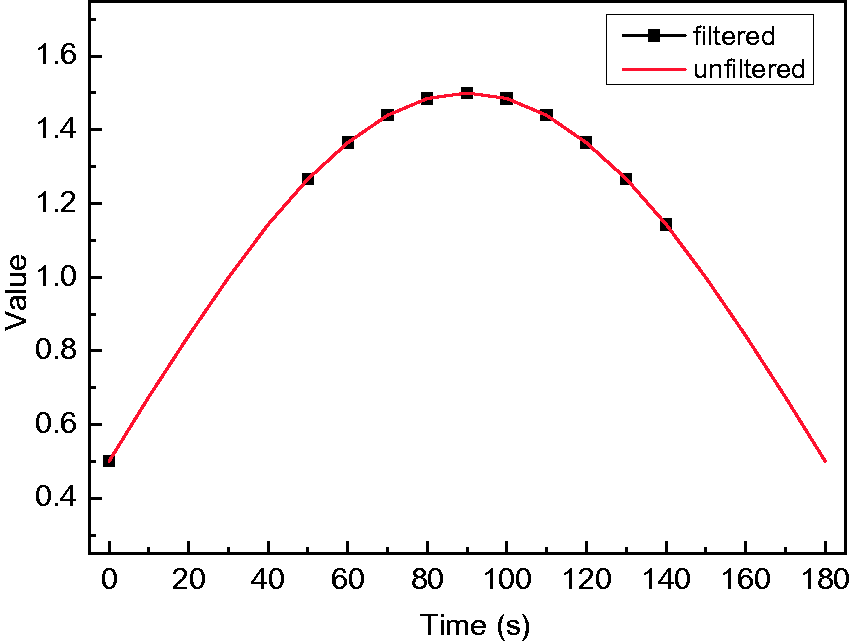
In this work, there are three layers in the NAR network, the input layer, the output layer, and the hidden layer. The number of neurons in the hidden layer is determined by

m = \sqrt{n + l} + a a \in [1, 10]

(14)

where n is the number of neurons in the input layer, l is the number of neurons in the output layer, and m is the number of neurons in the hidden layer.

In this paper, both the input layer and the output layer have only one neuron, so the number of neurons in the hidden layer is 1–11. Therefore, 11 NAR networks with different neurons in the hidden layer are trained and their mean square errors (MSEs) are compared. The network with the smallest MSE is the best one.

3.3. Reduce the discretization error by FEM

In equation (3), the force is broken into multiple rectangular pulses. In other words, the force is regarded as a constant at each $Δ t$ . The accuracy of this discrete method depends mainly on the size of $Δ t$ . The smaller $Δ t$ is, the more accurate the discrete force is. However, the smaller $Δ t$ is, the more expensive the computational cost of solving the equation is. Furthermore, small $Δ t$ may make $H$ ill-posed. Discretizing the force by using FEM can effectively reduce the discretization error. The force is broken into m elements in time domain. There are l nodes in each element. The interval between nodes is $Δ t$ . Then, the force in ith element can be expressed as

F_{i}^{h} (t) = \sum_{j = 1}^{l} q_{ij} (t) a_{ij} = q_{i}^{T} (t) a_{i} i = 1, 2, \dots, m

(15)

where

F_{i}^{h} (t)

is the approximation of the real force in the ith element,

q_{i}^{T} (t)

is the basis function vector in the ith element, and

a_{ij}

is the coefficient of jth basis function in the ith element.

Equation (15) can be rewritten as

F_{i}^{h} = Q_{i} a_{i}

(16)

where

Q_{i}

is a matrix of basic functions:

F_{i}^{h} = [\begin{matrix} \begin{matrix} F_{i}^{h} (t_{1}) & F_{i}^{h} \end{matrix} (t_{2}) & \begin{matrix} \dots & F_{i}^{h} (t_{l}) \end{matrix} \end{matrix}]^{T}

(17)

Q_{i} = [\begin{matrix} \begin{matrix} q_{i 1} (t_{1}) & q_{i 2} (t_{1}) \\ q_{i 1} (t_{2}) & q_{i 2} (t_{2}) \end{matrix} & \begin{matrix} \dots & q_{il} (t_{1}) \\ \dots & q_{il} (t_{2}) \end{matrix} \\ \begin{matrix} : & : \\ q_{i 1} (t_{l}) & q_{i 2} (t_{l}) \end{matrix} & \begin{matrix} : \\ \dots & q_{il} (t_{l}) \end{matrix} \end{matrix}]

(18)

The following equations can be derived from equation (16):

F^{h} = Θ a

(19)

Θ = diag [\begin{matrix} \begin{matrix} Q_{1} & Q_{2} \end{matrix} & \begin{matrix} \dots & Q_{m} \end{matrix} \end{matrix}]

(20)

Substituting equation (19) into equation (4),

R = (H Θ) a

(21)

Equation (6) can be rewritten as

J (λ, a) = ‖ R - (H Θ) a ‖ + λ a^{T} Φ a

(22)

Letting $Δ J = 0$ , equation (22) can be rewritten as

a = ((H Θ) T (H Θ) + λ Φ)^{- 1} (H Θ)^{T} R

(23)

The force can be reconstructed by equations (19) and (23). In this paper, the multi-quadric (MQ) basis function is used, which is given by

ϕ_{i} (x) = (c^{2} + d_{i}^{2})^{β}

(24)

where β and c are shape parameters, c is a constant (

c > 0

), β is an integer, and

d_{i}

denotes the distance from point

x

to point

x_{i}

, which can be expressed as

d_{i} = ‖ x - x_{i} ‖

. In this work,

c = Δ t

β = 2

, and the number of nodes in each element is 2.

4. Numerical simulation

In this section, an asymmetric plate and a 12-bay plane truss structure are used to validate the superiority of FFGM.

4.1. Numerical example 1: an asymmetric plate

4.1.1. The numerical model

The thickness of the plate is 3.4 mm and other dimensions are as shown in Figure 2. The Young modulus is 63.0 GPa. The density is 2730 $kg m^{3}$ . The Poisson ratio is 0.3. The damping of the plate is Rayleigh damping, the mass matrix coefficient is 0, and the stiffness matrix coefficient $β = 0.005$ . Point M1 is the excitation point and Point M2 is the measurement point. The shaded part is the fixed end. In engineering, there is noise in the measured signals. Consequently, it is necessary to add the artificial noise to the simulated data. The noise model is defined as additive white Gaussian noise with zero mean, which can be written as

N (t) = N_{d} e^{i 2 π η}

(25)

where i is a plural symbol, η is a uniformly distributed random number from 0 to 1, and

N_{d}

is a random number with a Gaussian distribution. The average value of

N_{d}

is 0 and the variance is determined by the following formula:

σ^{2} = S_{o} (t) \cdot 10^{- R / 20}

(26)

where

S_{o}

denotes the original signal and R denotes the signal-to-noise ratio (SNR).

In this numerical example, the width of the unit pulse is 10⁻³ s, and the excited force is expressed as

\begin{matrix} F (t) = {\begin{matrix} 10 \cdot sin (\frac{2 π t}{0.05}), 0 \leq x \leq 0.2 \\ x > 0.2 \end{matrix} \end{matrix}

(27)

4.1.2. Comparison of results with and without GA

$H_{δ}$ and $R_{δ}$ are obtained according to equation (3). Respectively, gradient descent (GD) and GA are used to get the regularization parameter α that minimizes $V (α)$ . Figure 3 shows the curves $V (α)$ when the SNR of the input signal is 10 dB and 20 dB. The regularization parameters, which are obtained by GD and GA, respectively, are marked in Figure 3. Figure 3(a) and (b) show the optimal regularization parameters when the SNR of the input signals is 10 dB and 20 dB, respectively.

As can be seen from Figure 3, compared with GD, GA can accurately find the minimum of $V (α)$ whether the SNR of the input signals is 10 dB or 20 dB. The accuracy of force identification is represented by the relative error between the identified force and the real force, which is defined as follows:

err = \frac{‖ F^{δ} - F_{0} ‖ 2}{‖ F_{0} ‖ 2} \times 100 %

(28)

where

F^{δ}

is the identified force and

F_{0}

is the real force.

The comparison of the forces identified by using GA and GD is shown in Figure 4.

Table 1 shows the relative errors between the identified forces and the real force.

Table 1.

The relative errors between the identified forces and the real force.

SNR (dB)	10	20
GA	39.24%	14.98%
GD	41.71%	15.10%

As can be seen from Figure 4 and Table 1, the accuracy of the force identified by GA is slightly higher than the force identified by GD. It indicates that GA is helpful to improve the accuracy of force identification by determining the minimum of $V (α)$ more accurately. The force is divided into two parts, sinusoidal part and zero part. In the sinusoidal part, the accuracy of the identified force at the peaks and valleys of the curve is lower than that of the rest of the curve. In the zero part, the identified force fluctuates greatly around the real force. There are high-frequency components in the identified forces, which are not found in the real force. The high-frequency components of the identified force are mainly generated by high-frequency noise in the input signals. It is noteworthy that the accuracy of the identified force when the SNR of the input signals is 20 dB is much higher than the accuracy of the identified force when the SNR of the input signals is 10 dB. It indicates that Tikhonov regularization has poor anti-noise performance.

4.1.3. The effect of the filter on the accuracy of force identification

It can be found from Section 4.1.2 that Tikhonov regularization has poor anti-noise performance. In this section, the filter is used to improve the anti-noise performance of Tikhonov regularization. In engineering, Gaussian white noise is the common noise. The Gaussian filter is commonly used to deal with Gaussian white noise. Therefore, we used the recursive Gaussian filter to suppress the noise of the input signals. However, the information of the initial and last segments of the filtered signals is lost when the recursive Gaussian filter is used to filter the signals. To deal with this problem, cubic spline interpolation and NAR network are introduced to repair the signals. The effect of the recursive Gaussian filter on the accuracy of the identified force is shown in Figure 5.

In Figure 5, TM is the traditional method. In TM, the force identified by Tikhonov regularization and the input signals are not filtered by the recursive Gaussian filter. The relative errors of the forces identified by the two methods are shown in Table 2.

Table 2.

The relative errors of the forces identified by the two methods.

SNR (dB)	10	20
TM	39.24%	14.98%
Filter	23.86%	10.50%

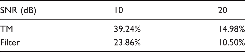
From Figure 5 and Table 2, it can be noted that the relative errors of the force identified by using the recursive Gaussian filter is less than the force identified by TM. It suggests that the recursive Gaussian filter can effectively reduce high-frequency noise of the input noise and improve the accuracy of the identified force.

4.1.4. FEM is used to improve the accuracy of the identified force

In this section, the effect of FEM is researched. Figure 6 shows the comparison between the forces identified by Filter, MQ FEM, and FFGM. In MQ FEM, the input signals are not filtered by the recursive Gaussian filter, the force is divided into several elements and the basis function is MQ. Each element has two nodes and the nodes are inside the element.

Table 3 shows the relative errors between the real force and the forces which are identified by the three methods, respectively.

Table 3.

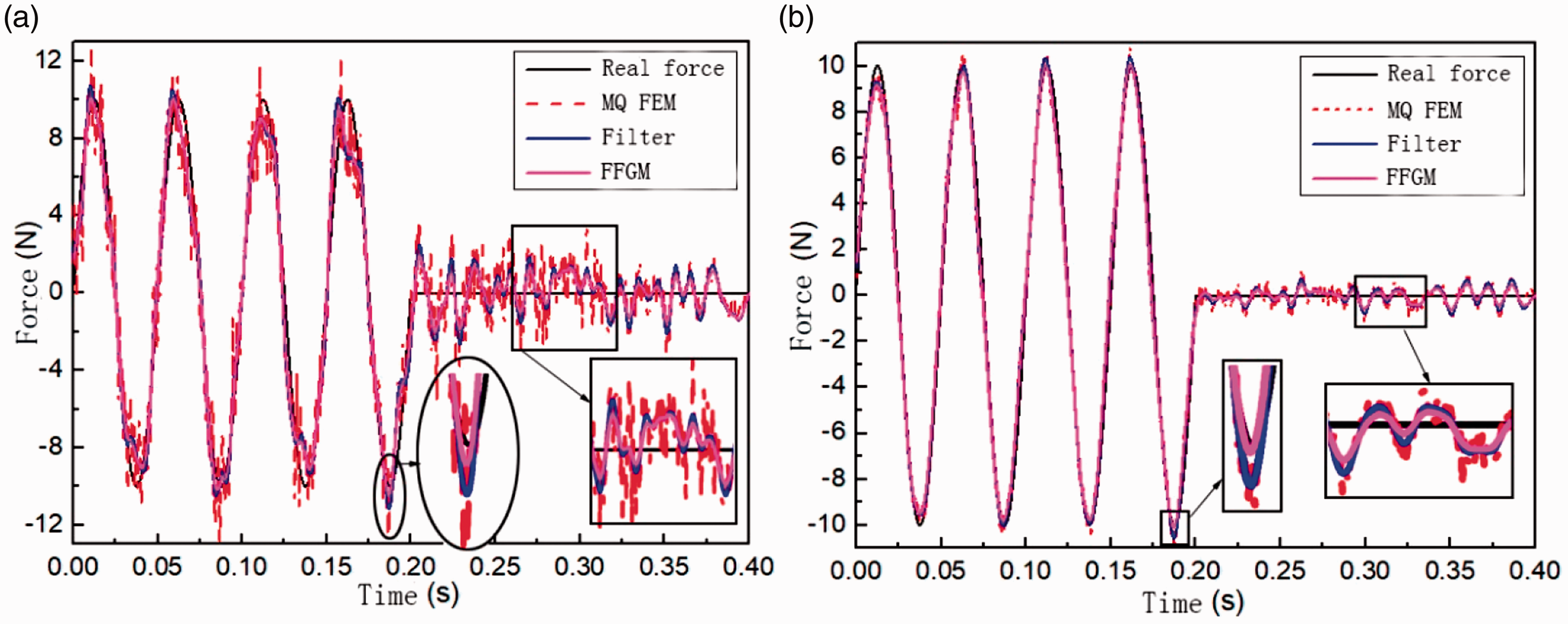
The relative errors of the forces identified by MQ FEM, filter, and FFGM.

SNR (dB)	TM	Filter	MQ FEM	FFGM
10	39.24%	23.86%	30.42%	19.13%
20	14.98%	10.50%	11.69%	9.92%

Obviously, the recursive Gaussian filter and MQ FEM can effectively improve the accuracy of the identified forces. The filter improves the accuracy of the identified force by reducing the noise of the input signals. MQ FEM improves the accuracy of the identified force by reducing the discretization error of the force. Therefore, FFGM, as a combination of filter and FEM, can further improve the accuracy of the identified force.

4.2. Numerical example 2: plane truss structure

4.2.1. The numerical model

A 12-bay plane truss structure is taken to investigate the effectiveness of the proposed FFGM for multi-force identification. There are 61 planar truss finite elements and 26 key points in the truss structure. As shown in Figure 7, Node 1 is pin-supported and Node 26 is roller-supported. The cross-sectional area of all straight bars is 0.0016 m², and the length of all horizontal and vertical bars is 1.0 m. The density and Young's modulus are 7.85e³ kg/m³ and 2.06 GPa, respectively. Assume that the two damping coefficients of Rayleigh damping are $α = 0.1523$ and $β = 4.6503$ e⁻⁴. The first eight natural frequencies of the structure are 1.579, 5.266, 7.066, 12.662, 18.500, 21.295, 29.016, and 32.349 Hz, respectively. There are only eight sensors for acceleration time history measurements and the sensors nodes are 4, 5, 10, 11, 16, 17, 22, and 23. The sampling frequency is 1000 Hz. Four sinusoidal loads F₁, F₂, F₃, and F₄, are applied vertically at nodes 3, 9, 15, and 21, respectively. The details of the four forces are shown as follows:

\begin{matrix} F_{1} (t) = 50 (1 - cos (10 π t)) sin (30 π t) \\ F_{2} (t) = 65 sin (20 π t) + 60 sin (80 π t) \\ + 55 sin (160 π t) \\ F_{3} (t) = 50 (1 - cos (20 π t)) sin (40 π t) \\ F_{4} (t) = 50 sin (18 π t) + 55 sin (70 π t) \\ + 50 sin (150 π t) \end{matrix}

(29)

A noise of 5% level is added to the measured responses before identifying the input force. All parameters and boundary conditions of this numerical model are the same as the one solved by Wang et al. (2015).

4.2.2. The result analysis

The input forces F₂ and F₄ identified by FFGM are compared with the real force and the results are shown in Figure 8. It can be seen from Figure 8 that the identified forces match the real forces very well.

FFGM is compared with the four methods, which are the Galerkin weak formulation (GW) (Wang et al., 2015), Tikhonov regularization method (TM), state space (Law and Yong, 2011), and Newmark (Liu et al., 2014) methods. The relative errors of the input forces identified by the five methods are shown in Table 4. From Table 4, it can be noted that the error of the force identified by FFGM is much less than the errors of the forces identified by other methods. It can be concluded that the proposed method named FFGM can effectively identify the multiple input forces with high accuracy.

Table 4.

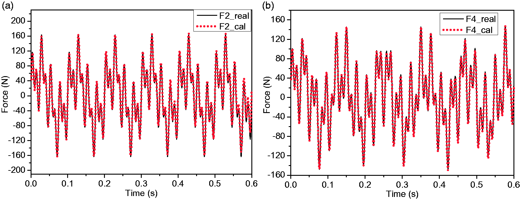
The relative errors of the input forces identified by the five methods.

Force	State space	Newmark	TM	GW	FFGM
F1	17.29%	17.07%	15.23%	14.08%	8.38%
F2	16.96%	12.38%	13.92%	10.26%	6.46%
F3	15.90%	14.42%	13.25%	12.19%	5.08%
F4	16.98%	10.42%	14.24%	8.62%	3.67%

5. Experimental verification

In Section 4, the performance of FFGM is verified by three numerical examples. FFGM has a good performance that it can accurately identify the input force. In this section, an experiment platform is designed to investigate the performance of FFGM in engineering.

5.1. The experiment platform

The experimental apparatus is shown in Figure 9. The experimental apparatus includes a particle damping composite plate, an acceleration transducer (Dytran3133B1), a power amplifier, a smart electromagnetic shaker (MTK2004E01), a force sensor (Dytran1051V4), and a dynamic signal analyzer (M+P SO Analyzer). A schematic diagram of the experimental object is shown in Figure 2.

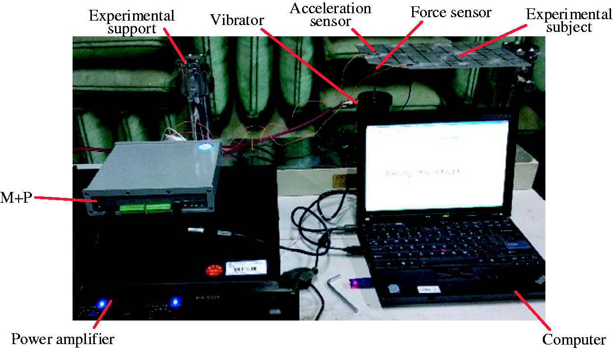
5.2. Analysis of results

The electromagnetic shaker applied sinusoidal excitation to M1, and the acceleration response of M2 was measured by the acceleration sensor. The unit pulse response and the acceleration response of the system were both obtained by experiments and they were used to identify the force by TM, MQ FEM, filter, and FFGM. The comparison of results is shown in Figure 10.

From Figure 10(a), the forces identified by TM and MQ FEM are similar to the real force and the forces identified by TM and MQ FEM are almost the same. The sampling rate in the experiment is 8192 Hz, which is already quite high, so the discretization error of TM is small. Therefore, the force identified by MQ FEM is almost the same as the force identified by TM. In addition, the force identified by TM and MQ FEM is significantly different from the real force at the peaks and valleys of the force-time history. Table 5 shows the relative errors between the forces identified by the four methods and the real force. From Table 4, the error of the force identified by MQ FEM is slightly smaller than that of the force identified by TM. By comparing Figure 10(a) with Figure 10(b), it can be found that the forces identified by Filter and FFGM match well with the real force. It proves that reducing the noise of the signal can effectively improve the accuracy of the identified force. The error of the force identified by FFGM is smaller than that of the force identified by Filter, which indicates that FFGM is more accurate.

Table 5.

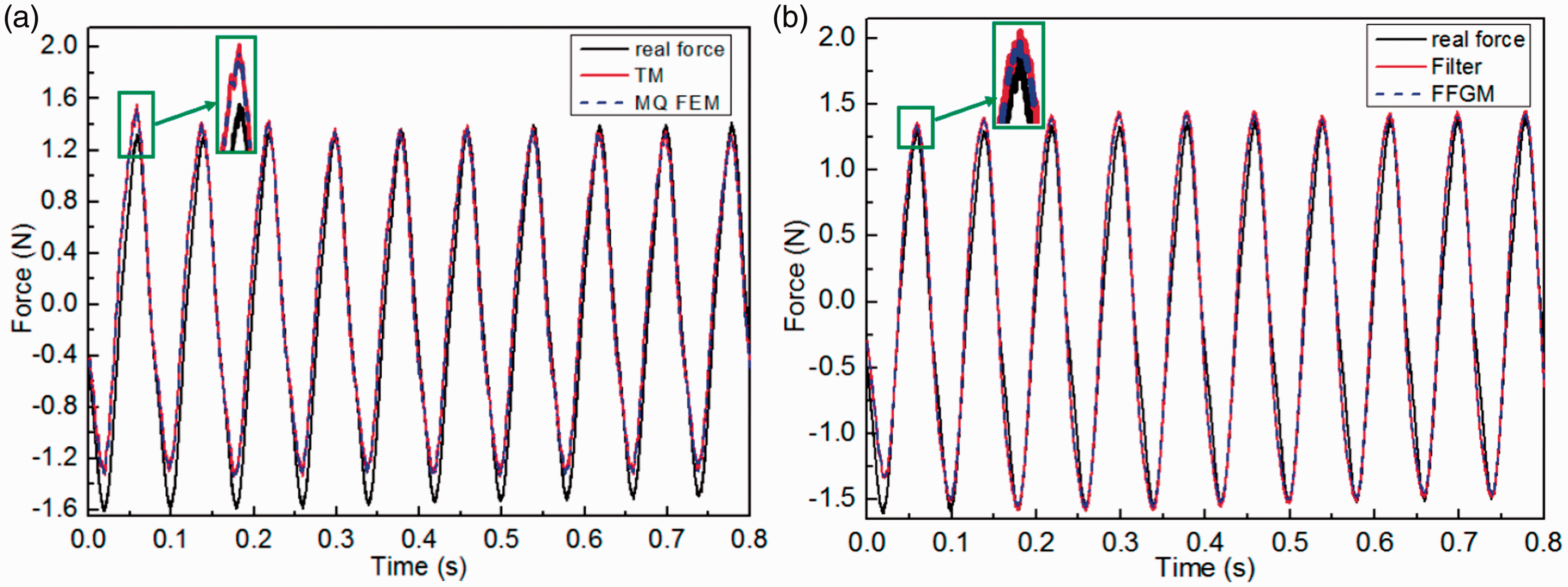
The relative errors of the four methods in experiment.

TM	Filter	MQ FEM	FFGM
5.66%	5.12%	5.38%	4.84%

6. Conclusions

In this paper, a novel method named FFGM is proposed to improve the accuracy of the identified force. The GA is used to determine the regularization parameter of GCV criterion. The filter combined with NAR and spline interpolation is used to suppress the noise of the input and MQ radial basis function is used to discretize the force to suppress the discretization error of the force. The superiority of FFGM is verified by three numerical examples and experiments. Compared with Tikhonov regularization, FFGM has good anti-noise performance and good accuracy.

Footnotes

Declaration of Conflicting Interests

The author(s) declared no potential conflicts of interest with respect to the research, authorship, and/or publication of this article.

Funding

The author(s) received no financial support for the research, authorship, and/or publication of this article.

References

Allen

(1971) Mean square error of prediction as a criterion for selecting variables. Technometrics 13: 469–475.

Aucejo

(2014) Structural source identification using a generalized Tikhonov regularization. Journal of Sound and Vibration 333: 5693–5707.

Aucejo

De Smet

(2018) An iterated multiplicative regularization for force reconstruction problems. Journal of Sound and Vibration 437: 16–28.

Aucejo

De Smet

Deu

(2019) On a space-time regularization for force reconstruction problems. Mechanical Systems and Signal Processing 118: 549–567.

De Deus

HPA

Da Silva

CRA

Jr Belo

, et al.(2012) The Tikhonov regularization method in elastoplasticity. Applied Mathematical Modelling 36: 4687–4707.

Golub

Heath

Wahba

(1979) Generalized cross-validation as a method for choosing a good ridge parameter. Technometrics 21: 215–223.

Hanke

Hansen

(1993) Regularization methods for large-scale problems. Surveys on Mathematics for Industry 3(4): 253–315.

Janssens

Gajdatsy

Gielen

, et al.(2011) OPAX: A new transfer path analysis method based on parametric load models. Mechanical Systems & Signal Processing 25: 1321–1338.

Jayalakshmi

Rao

ARM

(2017) Simultaneous identification of damage and input dynamic force on the structure for structural health monitoring. Structural and Multidisciplinary Optimization 55: 2211–2238.

10.

Jayalakshmi

Lakshmi

Mohan Rao

(2018) Dynamic force reconstruction techniques from incomplete measurements. Journal of Vibration and Control 24: 5321–5344.

11.

Kunisch

Zou

(1998) Iterative choices of regularization parameters in linear inverse problems. Inverse Problems 14: 34–40.

12.

Law

Yong

(2011) Substructure methods for structural condition assessment. Journal of Sound and Vibration 330: 3606–3619.

13.

(2018) Force localization and reconstruction using a two-step iterative approach. Journal of Vibration and Control 24: 3830–3841.

14.

Liu

Sun

Han

, et al.(2015) Dynamic load identification for stochastic structures based on Gegenbauer polynomial approximation and regularization method. Mechanical Systems & Signal Processing 56-57: 35–54.

15.

Liu

Law

Zhu

, et al.(2014) Explicit form of an implicit method for inverse force identification. Journal of Sound and Vibration 333: 730–744.

16.

Wang

(2005) Iterative implementation of the adaptive regularization yields optimality. Science in China 48: 55–62.

17.

Mao

Guo

Zhao

(2010) A state space force identification method based on Markov parameters precise computation and regularization technique. Journal of Sound and Vibration 329: 3008–3019.

18.

Menezes

JMP

Barreto

(2008) Long-term time series prediction with the NARX network: an empirical evaluation. Neurocomputing 71: 3335–3343.

19.

Morozov

(1984) Criteria for Selection of Regularization Parameter, New York: Springer.

20.

Prawin

Rao

ARM

(2018) An online input force time history reconstruction algorithm using dynamic principal component analysis. Mechanical Systems and Signal Processing 99: 516–533.

21.

Qiao

Chen

Xue

, et al.(2015) The application of cubic B-spline collocation method in impact force identification. Mechanical Systems & Signal Processing 64–65: 413–427.

22.

Qiao

Mao

Liu

, et al.(2019) Group sparse regularization for impact force identification in time domain. Journal of Sound and Vibration 445: 44–63.

23.

Qiao

Zhang

Gao

, et al.(2016a) Impact-force sparse reconstruction from highly incomplete and inaccurate measurements. Journal of Sound and Vibration 376: 72–94.

24.

Qiao

Zhang

Gao

, et al.(2017) Sparse deconvolution for the large-scale ill-posed inverse problem of impact force reconstruction. Mechanical Systems & Signal Processing 83: 93–115.

25.

Qiao

Zhang

Wang

, et al.(2016b) Sparse regularization for force identification using dictionaries. Journal of Sound and Vibration 368: 71–86.

26.

Ryzhikov

Biryulina

(1998) Sharp deconvolution in elimination of multiples. In: SEG Technical Program Expanded Abstracts, Tulsa, OK: Society of Exploration Geophysicists, pp. 1983–1986.

27.

Stevens KK (1987) Force identification problems: an overview. In: Proceedings of the 1987 SEM spring conference on experimental mechanics, Houston, TX, USA, 1987, pp.838-844.

28.

Tikhonov

(1963) On the solution of ill-posed problems and the method of regularization. Doklady Akademii Nauk SSSR 151(3): 501–504.

29.

Tikhonov

Goncharskiĭ

(1987) Ill-posed problems in the natural sciences, Moscow: Mir Publishers.

30.

Tveito

Langtangen

Nielsen

, et al.(2012) Parameter estimation and inverse problems. International Geophysics 67: 411–421.

31.

Wang

Wan

Wang

, et al.(2015) A novel state space method for force identification based on the Galerkin weak formulation. Computers & Structures 157: 132–141.

32.

Wang

Xiao

(2001) Fast realization algorithms for determining regularization parameters in linear inverse problems. Inverse Problems 17: 281.

33.

Wang

(2003) A restarted conjugate gradient method for ill-posed problems. Acta Mathematicae Applicatae Sinica 19: 31–40.