Vehicle–track interaction with consideration of rail irregularities at three-dimensional space

Abstract

Modelling of vehicle–track interaction has long been a hot and interesting topic. In multibody dynamics based on force-equilibrium methods, Hertzian contact and creep theories have been applied in vehicle–track model constructions. In another aspect, the complementarity-based methods have also been widely used in establishing vehicle–track interaction, but still having drawbacks on characterization of wheel–rail contact geometry/creepage in three-dimensional space. In this study, we draw essences from methodologies of refined wheel–rail coupling models and energy-variational principle, and a model for vehicle–track three-dimensional interactions with inclusion of rail irregularity excitations is newly developed. This model possesses high accuracy compared with Hertzian contact, FastSim, and vehicle–track coupled model in the middle-low frequency domain, and also, the advantages in computational stability are possessed. In this model, the unevenness of rail irregularities at the three-dimensional space is preliminarily considered by taking a hypothesis of normal distribution and accordingly, the wheel–rail three-dimensional constraint equations are presented. Extensively, a series of numerical examples are shown to verify the effectiveness and engineering practicability of this model. Besides, the influence of rail three-dimensional irregularities on the dynamic performance of vehicle–track systems is further explored, which shows when the trochoid of the wheel–rail contact points changes rapidly, the additional inertial effects brought out by rail irregularities might exert great influence on wheel–rail forces.

Keywords

Vehicle–track interactions rail irregularities wheel–rail contacts energy principle constraint equation

1. Introduction

The modelling of interactions between a vehicle and the tracks is critical for accurately predicting the system performances, quantitatively clarifying the time and frequency characteristics of dynamic indices and guiding the design of system parameters, etc. With the maturity of multibody dynamics, the approaches to characterize the interaction mechanism of vehicle subsystems, track subsystems, and most importantly, the wheel–rail interactions are multiple and are being chosen for various problem classes.

At the present stage, there are principally two contact models in multibody dynamics. One is the compliant contact force models, represented by Hertzian contact theory (Hertz, 1881) and its augments (Goldsmith, 1960; Hunt and Crossley, 1975; Xu et al., 2017), where the force reaction terms handing by spring-damper elements are explicitly used; the other is the complementarity models constructed on geometrical constraints (Brogliato, 1996; Panagiotopoulos, 1993), represented as a form of linear complementarity problem, which possess the properties that either the relative kinematics are zero, and the corresponding constraint forces are not zero or vice versa (Pfeiffer, 2003). In the vehicle–track multibody dynamics, the wheel–rail vertical interaction (two-dimensional (2-D) model) or the normal interaction (three-dimensional (3-D) model) is mainly depicted by the above two groups of methods. By combing with the wheel–rail tangential contact models (Johnson, 1999; Kalker, 1979, 1982), a series of work, see for instance, Zhai et al. (2009), Martínez-Casas et al. (2014), Torstensson et al. (2011), Giner-Navarro et al. (2018) and Dinh et al. (2009), etc., and many other fruitful researches have been achieved based on Hertz contact and creep theory.

Comparing with Hertz contacts that account for the wheel/rail relative indentation, the complementarity-based or similar methods have also received special attentions. With almost the same principle, Nielsen and Abrahamsson (1992) made an early work on formulating a constraint equation between vehicles and track, in which a moving vehicle with 4 degrees of freedom (DOFs) runs on a general three-parameter damped Winkler-type elastic foundation. Lee (1998) considered that the interaction force between a moving mass and the structure is determined by the velocity of the moving mass and the flexibility of structure. Neves et al. (2012) presented a vertical vehicle-structure interaction model, in which the equations of both systems are complemented with additional compatibility equations to ensure vehicle–structure contacts. In recent years, Stăncioiu et al. (2008), Cheng et al. (1999), Zhu et al. (2015) and Zhang et al. (2018), etc., also conducted extensive work on modelling interactions between moving vehicles and the guiding structures, where the methodologies on establishing constraint and governing equations for vehicle–substructure separations have been elaborated in various forms. However, all these studies have been limited in vertical (2-D) model, indicating the difficulties of implementing linear complementary method to 3-D dynamic scenarios if the separation phenomena are properly considered.

Except for the importance of modelling vehicle–track interactions, another necessity considered is the system excitation inputs. Rail irregularities, conventionally treated as the deviations of rail profiles from the standards, inevitably existed in wheel/rail interfaces, and generally rail irregularities play key roles in the quantification of the dynamic behaviours in addition to parametric excitations. However, the rail profile irregularities detected by track inspection car are conventionally regarded as the deformation of rail beams at 2-D space (Zeng et al., 2015), namely, the irregularities at the whole rail cross-section are the same; obviously, this is not in accordance with the real conditions: the profile deformations against the rail cross-section show unevenness, i.e. 3-D distribution characteristics. In recent years, Jin et al. (2016) and Zeng and Dimitrakopoulos (2018) made meaningful researches on investigating the train-bridge vibration performance under earthquakes, where the refinement wheel–rail contact models have been presented to depict the wheel derailment or jumping process. The wheel–rail tangential contact conforms with the nonlinear creep theory. As for the wheel–rail normal contact, Hertz contact theory has been used in the work of Jin et al., whereas unsmooth dynamics is used in the model of Zeng et al.

Summarily, it can be seen from the statement above that two issues should be dealt accordingly: one is the realization of vehicle–track dynamic interaction by complementarity methods with consideration of the wheel–rail normal/tangential contacts and separations simultaneously, the other is preliminarily figuring out the influence of rail 3-D irregularities. Following these two key problems, a novel model that combines the essences of a refinement wheel–rail coupling model (Zhai, 2015) in characterizing the wheel–rail contact geometry/creepage and the energy principle in deriving the dynamic equations of motion will be proposed. This model possesses higher computational stability and clearer physical concept.

2. Wheel–rail 3-D contacts

In this modelling framework, three assumptions are made as follows:

There is no elastic compression between the wheel and the rail;

The vehicle and the tracks are both linear systems;

Only rail irregularities with sampling interval larger than 0.25 m are considered;

$l_{\lim} \geq l_{a}$ , $l_{a}$ is the macro-axis of the contact ellipse, $l_{\lim}$ is the spatial interval of rail irregularities.

2.1. Wheel–rail constraint equations in 3-D contact

Let rail profile irregularities be non-uniformly distributed in 3-D space, denoted by $R (l, s)$ , where $l$ is the longitudinal distance along the rail line, $s$ is the rail cross-sectional coordinates. $l$ and $s$ are the functions of time $t$ regarding the moving of a train, and they are determined by the wheel–rail contact geometries in space.

At a constant time $t_{0}$ , the constraint equations for wheel–rail contacts can be expressed by

Z_{w_{i}} (l (t), s (t)) = {[Z_{r} (l_{i}, s_{i}) + R (l_{i}, s_{i})] |}_{t = t_{0}}

(1)

{\dot{Z}}_{w_{i}} (l (t), s (t)) = {[\frac{\partial Z_{r} (l_{i}, s_{i})}{\partial l_{i}} V + \frac{\partial Z_{r} (l_{i}, s_{i})}{\partial s_{i}} {\dot{s}}_{i} + \frac{\partial R (l_{i}, s_{i})}{\partial l_{i}} V + \frac{\partial R (l_{i}, s_{i})}{\partial s_{i}} {\dot{s}}_{i}] |}_{t = t_{0}}

(2)

{\ddot{Z}}_{w_{i}} (l (t), s (t)) = {[\begin{array}{l} \frac{\partial^{2} Z_{r} (l_{i}, s_{i})}{\partial l_{i}^{2}} V^{2} + 2 \frac{\partial^{2} Z_{r} (l_{i}, s_{i})}{\partial l_{i} \partial s_{i}} V {\dot{s}}_{i} + \frac{\partial Z_{r} (l_{i}, s_{i})}{\partial l_{i}} a + \frac{\partial^{2} Z_{r} (l_{i}, s_{i})}{\partial s_{i}^{2}} {\dot{s}}_{i}^{2} + \frac{\partial Z_{r} (l_{i}, s_{i})}{\partial s_{i}} {\ddot{s}}_{i} + \\ \frac{\partial^{2} R (l_{i}, s_{i})}{\partial l_{i}^{2}} V^{2} + 2 \frac{\partial^{2} R (l_{i}, s_{i})}{\partial l_{i} \partial s_{i}} {\dot{s}}_{i} V + \frac{\partial R (l_{i}, s_{i})}{\partial l_{i}} a + \frac{\partial^{2} R (l_{i}, s_{i})}{\partial s_{i}^{2}} {\dot{s}}_{i}^{2} + \frac{\partial R (l_{i}, s_{i})}{\partial s_{i}} {\ddot{s}}_{i} \end{array}] |}_{t = t_{0}}

(3)

where

i = 1,2,3,4

denote the ith wheel–rail contact point; the subscript ‘w’ and ‘r’ denote the wheelset and the rail, respectively;

V

and

a

denote the vehicle velocity and acceleration, respectively,

a = 0

when a train runs with a constant velocity;

{\dot{s}}_{i}

and

{\ddot{s}}_{i}

, respectively, denote the velocity and the acceleration of the wheel–rail contact point at the reference frame of the global coordinate system; the dot above symbol denotes differentiation with respect to time

t

; and

Z_{w}

and

Z_{r}

are the wheel and rail vertical displacement, respectively.

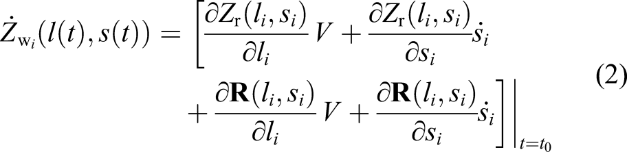
2.2. Wheel–rail vertical interaction

The negative value of the work done by the inertial force of a wheelset can be obtained by the following equation

V_{F, m} = \sum_{j = 1}^{4} m_{w} {\ddot{Z}}_{w, j, r} Z_{w, j, r}

(4)

with

\begin{array}{l} {\ddot{Z}}_{w, j, r} = \frac{1}{2} \sum_{r} N_{v, j, r} {[\begin{matrix} {\ddot{Z}}_{r, j, r} & {\ddot{R}}_{j, r} \end{matrix}]}^{T}, Z_{r, j, r} (l, s) = \sum_{i = V, θ} N_{i, j, r} Φ_{r z, j, r}, \\ N_{v, j, r} = [\begin{matrix} 1 & 1 \end{matrix}], \\ N_{V, j, r} = {[\begin{matrix} 0 & 1 - 3 {\tilde{l}}^{2} + 2 {\tilde{l}}^{3} & - (\tilde{l} - 2 {\tilde{l}}^{2} + {\tilde{l}}^{3}) L_{l} & 3 {\tilde{l}}^{2} - 2 {\tilde{l}}^{3} & - ({\tilde{l}}^{3} - {\tilde{l}}^{2}) L_{l} & 0 \end{matrix}]}_{\hat{l} = l_{a} / L_{l}}, \\ N_{θ, j, r} = (b_{0} - s_{j, r}^{'}) {[\begin{matrix} 1 - \tilde{l} & 0 & 0 & 0 & 0 & \tilde{l} \end{matrix}]}_{\hat{l} = l_{a} / L_{l}}, \\ Φ_{r z, j, r} = {[\begin{matrix} θ_{r x, r, 1} & z_{r, r, 1} & θ_{r y, r, 1} & z_{r, r, 2} & θ_{r y, r, 2} & θ_{r x, r, 2} \end{matrix}]}^{T}, \end{array}

where

N

denotes the equivalent shape function;

Φ

denotes the DOF corresponding to the shape function;

s_{j, r}^{'}

is the semi-lateral distance between wheel–rail contact positions time-dependently;

m_{w}

is the mass of a wheelset;

L_{l}

is the length of a rail beam element;

l_{a}

is the distance between the left node of the rail beam element and the contact position;

z_{r}

θ_{r y}

, and

θ_{r x}

denote the rail vertical displacement and rail angular displacements around Y- and X-axis, respectively; the subscripts ‘1’ and ‘2’ denote the left- and right-node of rail beam element, respectively;

b_{0}

denotes the initial semi-lateral distance between the two contact points in a wheelset; and

j = 1,2,3,4

denote the

j th

wheelset.

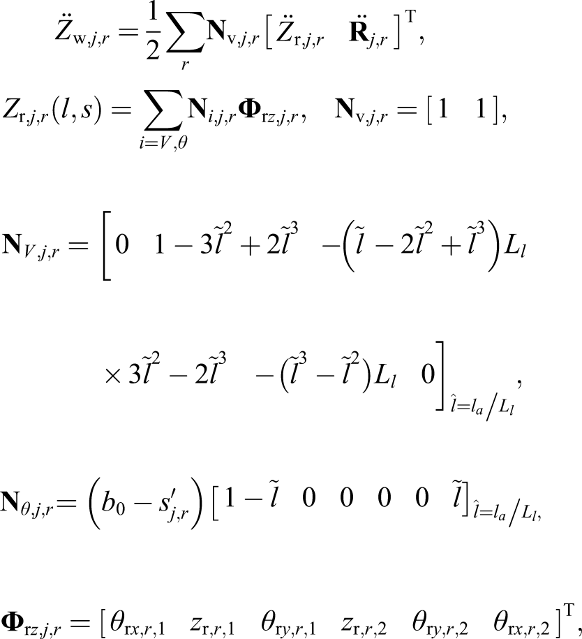
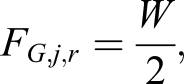
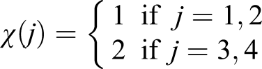
From equations (1) to (4), it can be derived that the motion of a wheelset is closely correlated with the rail vibrations. Besides, the wheel–rail vertical force can be calculated by d’Alembert principle, that is (Xu and Zhai, 2020a)

F_{w, j, r} = F_{ϕ, j, r} + F_{z, j, r} + F_{G, j, r}

(5)

with

F_{ϕ, j, r} = {(- 1)}^{r + 1} [\begin{array}{l} (\frac{m_{c} {\ddot{y}}_{c}}{8 b_{0}} + {(- 1)}^{χ (j) + 1} \frac{I_{c z} {\ddot{ψ}}_{c}}{8 l_{c} b_{0}}) (H_{c b} + H_{b t} + H_{t w} + R_{w}) + \frac{I_{c x} {\ddot{ϕ}}_{c}}{8 b_{0}} + \frac{m_{b} {\ddot{y}}_{b, j}}{4 b_{0}} (H_{t w} + R_{w}) + \\ \frac{I_{b x} {\ddot{ϕ}}_{b, j}}{4 b_{0}} + {(- 1)}^{j + 1} \frac{I_{b z} {\ddot{ψ}}_{b, j}}{2 l_{t}} \frac{H_{t w} + R_{w}}{2 b_{0}} + \frac{I_{w x} {\ddot{ϕ}}_{w}}{2 b_{0}} \end{array}],

F_{z, j, r} = - \frac{m_{c} {\ddot{z}}_{c}}{8} - \frac{m_{b} {\ddot{z}}_{b, j}}{4} + {(- 1)}^{χ (j) + 1} \frac{I_{c y} {\ddot{β}}_{c}}{8 l_{c}} + {(- 1)}^{j + 1} \frac{I_{b y} {\ddot{β}}_{b, j}}{4 l_{t}} - m_{w, j, r} {\ddot{z}}_{w, j, r},

F_{G, j, r} = \frac{W}{2},

χ (j) = {\begin{cases} 1 if j = 1,2 \\ 2 if j = 3,4 \end{cases}

where

F_{ϕ}

F_{z}

, and

F_{G}

, respectively, denote the wheel–rail force induced by the rolling, bounce, and gravitational effect of the vehicle;

m

denotes the mass of a body;

I_{x}

I_{y}

, and

I_{z}

denote the moment of inertia of a body around the X-, Y-, and Z-axis, respectively; when

j = 1,2

{\ddot{y}}_{b, j}

{\ddot{ψ}}_{b, j}

{\ddot{ϕ}}_{b, j}

, and

{\ddot{β}}_{b, j}

, respectively, denote the lateral, yaw, rolling, and pitch acceleration of the front bogie frame, whereas

j = 3,4

correspond to the acceleration of the rear bogie frame; the subscripts “c,” “b,” and “w,” respectively, denote the car body, the bogie frame, and the wheelset;

R_{w}

is the radius of rolling circle of a wheel;

H_{cb}

is the vertical distance between the centroid of the car body and the upper surface of the secondary suspension;

H_{bt}

is the vertical distance between the centroid of a bogie frame and the lower surface of the secondary suspension;

H_{tw}

is the vertical distance between the centroids of the bogie frame and the wheelset; and

W

is the static axle load.

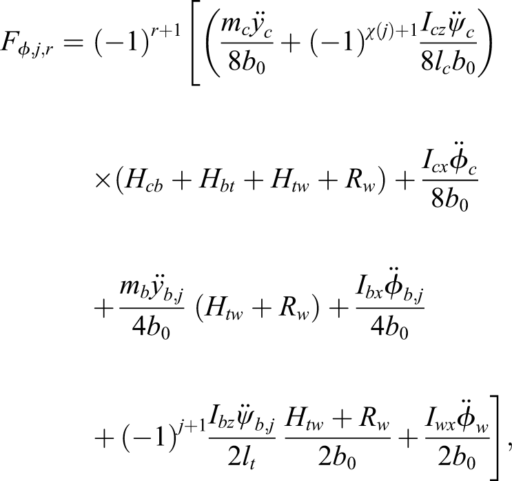
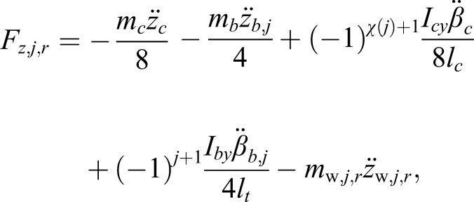
2.3. Wheel–rail lateral interaction (Xu et al., 2020a, 2020b)

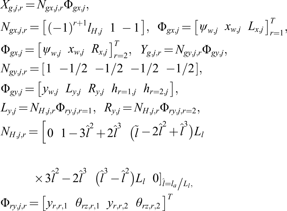
In the consideration of wheel–rail lateral interactions, an investigation of the wheel–rail nonlinear and time-variant creepage should be further conducted.

Because of the intrinsic feature of wheel profile treads, the work done by the restoring force of the vehicle can be expressed by

V_{F, g} = \sum_{j = 1}^{4} \sum_{r} \frac{1}{2} (k_{g}^{X} X_{g, j, r}^{2} + k_{g}^{Y} Y_{g, j, r}^{2})

(6)

with

\begin{array}{l} X_{g, j, r} = N_{g x, j, r} Φ_{g x, j}, \\ N_{g x, j, r} = [\begin{matrix} {(- 1)}^{r + 1} l_{H, j} & 1 & - 1 \end{matrix}], Φ_{g x, j} = {[\begin{matrix} ψ_{w, j} & x_{w, j} & L_{x, j} \end{matrix}]}_{r = 1}^{T}, Φ_{g x, j} = {[\begin{matrix} ψ_{w, j} & x_{w, j} & R_{x, j} \end{matrix}]}_{r = 2}^{T}, \\ Y_{g, j, r} = N_{g y, j, r} Φ_{g y, j}, \\ N_{g y, j, r} = [\begin{matrix} 1 & - 1 / 2 & - 1 / 2 & - 1 / 2 & - 1 / 2 \end{matrix}], Φ_{g y, j} = [\begin{matrix} y_{w, j} & L_{y, j} & R_{y, j} & h_{r = 1, j} & h_{r = 2, j} \end{matrix}], \\ L_{y, j} = N_{H, j, r} Φ_{r y, j, r = 1}, R_{y, j} = N_{H, j, r} Φ_{r y, j, r = 2}, \\ N_{H, j, r} = {[\begin{matrix} 0 & 1 - 3 {\hat{l}}^{2} + 2 {\hat{l}}^{3} & (\tilde{l} - 2 {\hat{l}}^{2} + {\hat{l}}^{3}) L_{l} & 3 {\hat{l}}^{2} - 2 {\hat{l}}^{3} & ({\hat{l}}^{3} - {\hat{l}}^{2}) L_{l} & 0 \end{matrix}]}_{\hat{l} = l_{a} / L_{l},} \\ Φ_{r y, j, r} = {[\begin{matrix} y_{r, r, 1} & θ_{r z, r, 1} & y_{r, r, 2} & θ_{r z, r, 2} \end{matrix}]}^{T} \end{array}

where

k_{g}^{X}

and

k_{g}^{Y}

are, respectively, the equivalent angular stiffness of wheel–rail contact and the equivalent stiffness of gravity (Wang, 1994);

ψ_{w}

denotes the yaw angle of a wheelset;

x_{w}

and

y_{w}

denote the longitudinal and lateral displacement of the wheelset;

L_{x}

and

R_{x}

denote the rail longitudinal displacement at the contact point;

h_{r, j}

denotes the rail lateral irregularity at the contact point;

y_{r}

and

θ_{r z}

denote the node lateral displacement and angle around Z-axis, respectively; and

l_{H, j}

denotes half of the lateral distance between the two contact points of the

j th

wheelset.

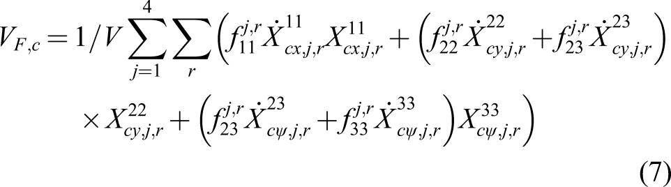
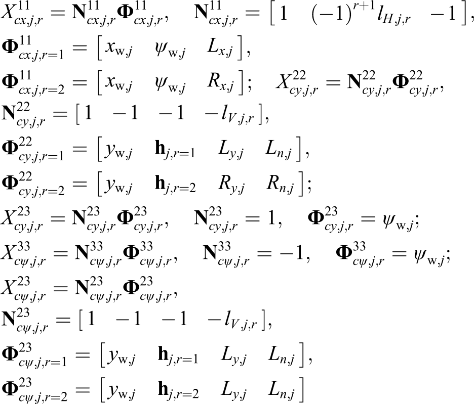
Obviously, the negative value of the work done by the wheel–rail creep forces, represented by $V_{F, c}$ , can be expressed by

V_{F, c} = 1 / V \sum_{j = 1}^{4} \sum_{r} (f_{11}^{j, r} {\dot{X}}_{c x, j, r}^{11} X_{c x, j, r}^{11} + (f_{22}^{j, r} {\dot{X}}_{c y, j, r}^{22} + f_{23}^{j, r} {\dot{X}}_{c y, j, r}^{23}) X_{c y, j, r}^{22} + (f_{23}^{j, r} {\dot{X}}_{c ψ, j, r}^{23} + f_{33}^{j, r} {\dot{X}}_{c ψ, j, r}^{33}) X_{c ψ, j, r}^{33})

(7)

with

\begin{array}{l} X_{c x, j, r}^{11} = N_{c x, j, r}^{11} Φ_{c x, j, r}^{11}, N_{c x, j, r}^{11} = [\begin{matrix} 1 & {(- 1)}^{r + 1} l_{H, j, r} & - 1 \end{matrix}], \\ Φ_{c x, j, r = 1}^{11} = [\begin{matrix} x_{w, j} & ψ_{w, j} & L_{x, j} \end{matrix}], Φ_{c x, j, r = 2}^{11} = [\begin{matrix} x_{w, j} & ψ_{w, j} & R_{x, j} \end{matrix}]; \\ X_{c y, j, r}^{22} = N_{c y, j, r}^{22} Φ_{c y, j, r}^{22}, N_{c y, j, r}^{22} = [\begin{matrix} 1 & - 1 & - 1 & - l_{V, j, r} \end{matrix}], \\ Φ_{c y, j, r = 1}^{22} = [\begin{matrix} y_{w, j} & h_{j, r = 1} & L_{y, j} & L_{n, j} \end{matrix}], Φ_{c y, j, r = 2}^{22} = [\begin{matrix} y_{w, j} & h_{j, r = 2} & R_{y, j} & R_{n, j} \end{matrix}]; \\ X_{c y, j, r}^{23} = N_{c y, j, r}^{23} Φ_{c y, j, r}^{23}, N_{c y, j, r}^{23} = 1, Φ_{c y, j, r}^{23} = ψ_{w, j}; \\ X_{c ψ, j, r}^{33} = N_{c ψ, j, r}^{33} Φ_{c ψ, j, r}^{33}, N_{c ψ, j, r}^{33} = - 1, Φ_{c ψ, j, r}^{33} = ψ_{w, j}; \\ X_{c ψ, j, r}^{23} = N_{c ψ, j, r}^{23} Φ_{c ψ, j, r}^{23}, N_{c ψ, j, r}^{23} = [\begin{matrix} 1 & - 1 & - 1 & - l_{V, j, r} \end{matrix}], \\ Φ_{c ψ, j, r = 1}^{23} = [\begin{matrix} y_{w, j} & h_{j, r = 1} & L_{y, j} & L_{n, j} \end{matrix}], Φ_{c ψ, j, r = 2}^{23} = [\begin{matrix} y_{w, j} & h_{j, r = 2} & L_{y, j} & L_{n, j} \end{matrix}] \end{array}

where

f_{11}^{j, r}

f_{22}^{j, r}

f_{23}^{j, r}

, and

f_{33}^{j, r}

denote the creep coefficients at the wheel/rail interfaces; the superscript “

j

” denotes the jth wheelset and the superscript “r” denotes the wheel–rail contact side;

V

is the nominal rolling speed;

l_{V, j, r}

is the vertical distance between the wheel/rail contact point and the rail centroid; and

L_{n, j}

and

R_{n, j}

denote the rail torsional angles at the contact point.

3. Vehicle–track 3-D coupling interactions

The vehicle–track (3-D) dynamic model, as shown in Figure 1, is treated as a vehicle running on the ballasted tracks with a constant velocity.

Figure 1.

Train-track systems (a) side view and (b) end view.

For constructing the vehicle–track coupling interactions in 3-D space, the work, elastic strain, and potential energy produced in the vehicle–track interactions should be further presented except the work done by the wheel/rail related forces.

3.1. Work/energy representations for vehicle elastic systems

The work and energy in the vehicle elastic system can be represented by the work done by the gravitational forces and damping forces, and the elastic deformational energy done by spring forces in suspension systems.

3.1.1. The negative value of the work done by the inertial forces

The negative value of the work by inertial forces can be expressed by

V_{v, m} = \sum_{u} m_{u} {\ddot{X}}_{u} X_{u}

(8)

where the subscript “u” denotes the vehicle component, i.e. the car body and the bogie frames;

m_{u}

represents the mass or the moment of inertia of the vehicle bodies.

3.1.2. The negative value of the work done by the damping forces

The negative value of the work induced by the damping forces can be expressed by

V_{v, c} = \sum_{q} c_{q} {\dot{X}}_{q} X_{q}

(9)

with

X_{q} = N_{v, c, q} X_{q}, {\dot{X}}_{q} = N_{v, c, q} {\dot{X}}_{q}

, where the subscript “q” denotes the suspension component, i.e. the two-stage suspension components;

c_{q}

is the coefficient of damping;

N_{v, c, q}

is the equivalent shape function characterizing the deformational displacement/velocity of suspension components, the detail expressions of which can be consulted in Xu et al. (2020b); and

X_{q}

and

{\dot{X}}_{q}

are, respectively, the displacement and velocity of DOF related to the relative motions.

3.1.3. The elastic deformational energy

The negative value of the work induced by the damping forces can be expressed by

V_{v, e} = \frac{1}{2} \sum_{q} k_{q} X_{q}^{2}

(10)

where

k_{q}

denotes the coefficient of stiffness.

3.2. Work/energy representations for track elastic systems

The work and energy done in a ballasted-track system can be represented by the potential energy of the inertial forces, the elastic strain energy and the work done by the rail-sleeper, the sleeper-ballast bed, and the ballast bed-subgrade interactions.

3.2.1. The potential energy of the inertial forces

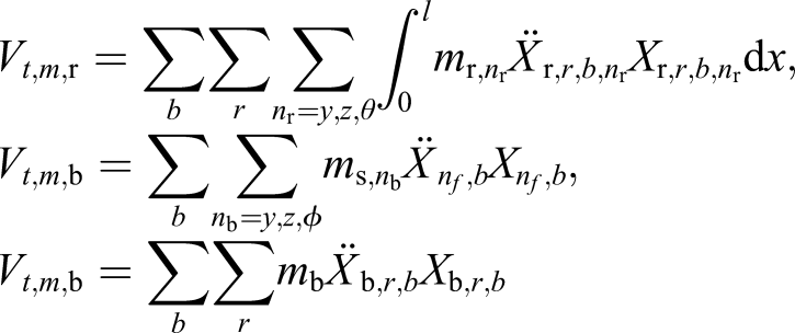
The negative value of the potential energy of the inertial force can be expressed by

V_{t, m} = V_{t, m, r} + V_{t, m, s} + V_{t, m, b}

(11)

with

\begin{array}{l} V_{t, m, r} = \sum_{b} \sum_{r} \sum_{n_{r} = y, z, θ} \int_{0}^{l} m_{r, n_{r}} {\ddot{X}}_{r, r, b, n_{r}} X_{r, r, b, n_{r}} d x, \\ V_{t, m, b} = \sum_{b} \sum_{n_{b} = y, z, ϕ} m_{s, n_{b}} {\ddot{X}}_{n_{f}, b} X_{n_{f}, b}, \\ V_{t, m, b} = \sum_{b} \sum_{r} m_{b} {\ddot{X}}_{b, r, b} X_{b, r, b} \end{array}

where

m_{r, n_{r}}

is the mass of the rail per unit length or the moment of inertia around X-axis;

m_{s, n_{b}}

is the mass or moment of inertia corresponding to the DOFs of the sleeper;

m_{b}

is the mass of the ballast bed;

n_{r} = y, z, ϕ

denotes the lateral, vertical, and rotation around the X-axis motion of the rail;

n_{b} = y, z, ϕ

denotes the lateral, vertical, and rotation around the X-axis motion of the sleeper;

b

denotes the number of the track element;

X_{r, r, b, n_{r}}

is the displacement vector the rail element;

X_{n_{f}, b}

and

X_{b, r, b}

, respectively, denote the displacement or rotational angle of the sleeper and the vertical displacement of the ballast bed; and

l

is the length of a rail element.

3.2.2. The elastic potential energy

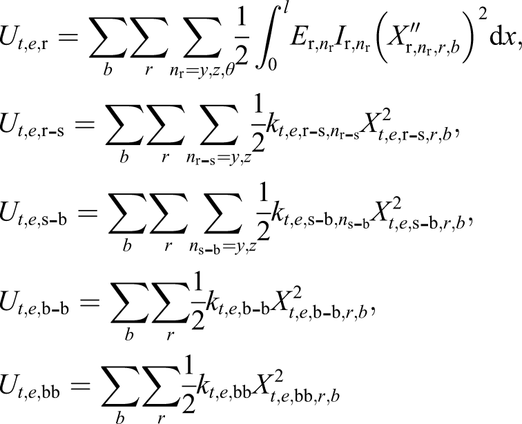
The elastic potential energy of the track system consists of the rail strain energy and the elastic deformation energy of the springs, namely

U_{t, e} = U_{t, e, r} + U_{t, e, r ‐ s} + U_{t, e, s ‐ b} + U_{t, e, b ‐ b} + U_{t, e, bb}

(12)

with

\begin{array}{l} U_{t, e, r} = \sum_{b} \sum_{r} \sum_{n_{r} = y, z, θ} \frac{1}{2} \int_{0}^{l} E_{r, n_{r}} I_{r, n_{r}} {(X_{r, n_{r}, r, b}^{''})}^{2} d x, \\ U_{t, e, r ‐ s} = \sum_{b} \sum_{r} \sum_{n_{r ‐ s} = y, z} \frac{1}{2} k_{t, e, r ‐ s, n_{r ‐ s}} X_{t, e, r ‐ s, r, b}^{2}, U_{t, e, s ‐ b} = \sum_{b} \sum_{r} \sum_{n_{s ‐ b} = y, z} \frac{1}{2} k_{t, e, s ‐ b, n_{s ‐ b}} X_{t, e, s ‐ b, r, b}^{2}, \\ U_{t, e, b ‐ b} = \sum_{b} \sum_{r} \frac{1}{2} k_{t, e, b ‐ b} X_{t, e, b ‐ b, r, b}^{2}, U_{t, e, bb} = \sum_{b} \sum_{r} \frac{1}{2} k_{t, e, bb} X_{t, e, bb, r, b}^{2} \end{array}

where

E_{r, n_{r}}

is the elastic modulus of the rail when

n_{r} = y, z

, the rail shearing modulus when

n_{r} = θ

;

I_{r, n_{r}}

is the moment of inertia of rail cross-section around Z- and Y-axis, respectively, when

n_{r} = y, z

, and the torsional moment of inertia when

n_{r} = θ

; the prime denotes differentiation with respect to the local coordinate of rail element;

k_{t, e, r ‐ s, n_{r ‐ s}}

denotes the lateral and vertical stiffness coefficient between the rail and the sleeper corresponding to

n_{r ‐ s} = y, z

, respectively;

k_{t, e, s ‐ b, n_{s ‐ b}}

denotes the lateral stiffness coefficient between the sleeper and the subgrade and the vertical stiffness coefficient between the sleeper and the ballast bed, respectively;

k_{t, e, b ‐ b}

denotes the shear stiffness coefficient between the ballast beds;

k_{t, e, bb}

denotes the vertical stiffness between the ballast bed and the subgrade; and

X_{t, e}

denotes the elastic deformation of springs.

3.2.3. The work done by the damping forces

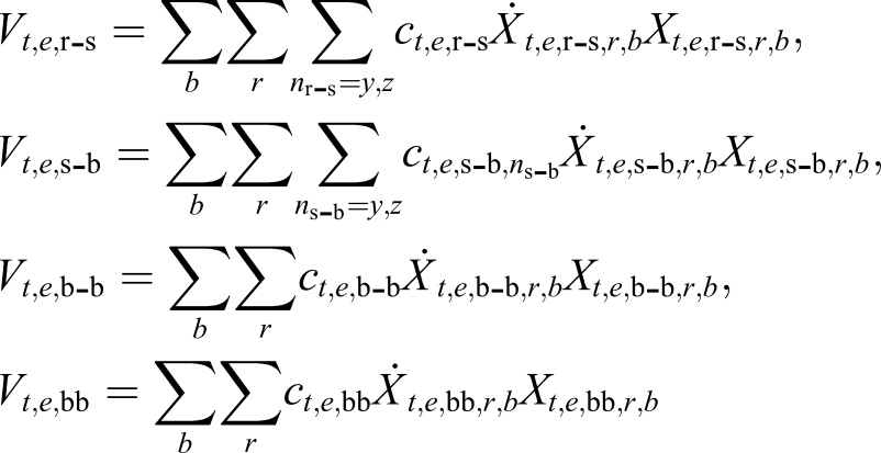
The negative value of the work done by the damping forces can be expressed by

V_{t, c} = V_{t, e, r ‐ s} + V_{t, e, s ‐ b} + V_{t, e, b ‐ b} + V_{t, e, bb}

(13)

with

\begin{array}{l} V_{t, e, r ‐ s} = \sum_{b} \sum_{r} \sum_{n_{r ‐ s} = y, z} c_{t, e, r ‐ s} {\dot{X}}_{t, e, r ‐ s, r, b} X_{t, e, r ‐ s, r, b}, V_{t, e, s ‐ b} = \sum_{b} \sum_{r} \sum_{n_{s ‐ b} = y, z} c_{t, e, s ‐ b, n_{s ‐ b}} {\dot{X}}_{t, e, s ‐ b, r, b} X_{t, e, s ‐ b, r, b}, \\ V_{t, e, b ‐ b} = \sum_{b} \sum_{r} c_{t, e, b ‐ b} {\dot{X}}_{t, e, b ‐ b, r, b} X_{t, e, b ‐ b, r, b}, V_{t, e, bb} = \sum_{b} \sum_{r} c_{t, e, bb} {\dot{X}}_{t, e, bb, r, b} X_{t, e, bb, r, b} \end{array}

where

c

denotes the damping coefficient. The other parameters have the same meaning as those in equation (12).

3.3. Formation of vehicle–track coupling matrices

The total potential energy of an elastic system can be expressed by

Π_{d} = V_{F, m} + V_{F, g} + V_{F, c} + V_{v, m} + V_{v, c} + V_{t, e} + V_{t, m} + U_{t, e} + V_{t, c}

(14)

Based on principles of virtual work and d’Alembert and considering the damping force, equation (14) must satisfy (Bleich, 1952)

δ_{\in} Π_{d} = 0

(15)

where

δ

is the variational symbol; the subscript “

\in

” indicates that the variation of

Π_{d}

aims only at the elastic strain and displacement vectors to guarantee the nature of virtual work principle.

Equation (15) is a corollary of the d’Alembert principle when fixing the time $t$ transiently and accordingly, it can be regarded that $Π_{d}$ is only the function of displacement and strain vector $u$ for an elastic dynamic system. Obviously, for a dynamical system with $n$ independent displacement coordinates $u_{i} (i = 1,2, ..., n)$ , it can be deduced as

\sum_{i = 1}^{n} \frac{\partial_{\in} Π_{d}}{\partial u_{i}} δ u_{i} = 0

(16)

In equation (16), $δ u_{i} \neq 0$ , thus $\partial_{\in} Π_{d} / \partial u_{i} = 0$ and of necessary it represents the $i th$ dynamic equilibrium equation, which consist of displacement $u_{j}$ , $j = 1,2, ..., n$ . In the matrices derived, the serial number $u_{j}$ and $δ u_{i}$ , respectively, indicate the position of the coefficient at the $j th$ column and the $i th$ row of the matrix, which is technically developed by a “set-in-right-position” rule in Zeng and Yang (1986).

The dynamic equations of motion for vehicle–track systems can be accordingly derived by equations (14)–(16) as follows

[\begin{matrix} M_{v v} & M_{v t} \\ M_{t v} & M_{t t} \end{matrix}] [\begin{array}{l} {\ddot{X}}_{v} \\ {\ddot{X}}_{t} \end{array}] + [\begin{matrix} C_{v v} & C_{v t} \\ C_{t v} & C_{t t} \end{matrix}] [\begin{array}{l} {\dot{X}}_{v} \\ {\dot{X}}_{t} \end{array}] + [\begin{matrix} K_{v v} & K_{v t} \\ K_{t v} & K_{t t} \end{matrix}] [\begin{array}{l} X_{v} \\ X_{t} \end{array}] = F_{e x t} + F_{R, h}

(17)

where the subscript “v” and “t” denote the vehicle and the track, respectively;

M

C

, and

K

denote the mass, damping, and stiffness matrix, respectively, and

F

denotes the load vectors.

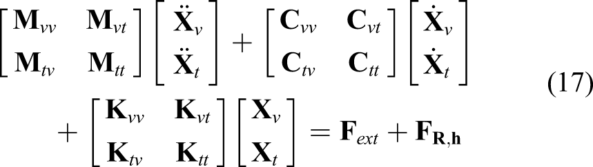
In equation (17), it can be observed that vehicle and the tracks are wholly coupled as an entire system no matter on displacement complementarity and on force equilibrium. $F_{e x t}$ is derived from the external excitations, including system gravity, and the loads transformed from rail irregularities, namely, $F_{R, h}$ , can be obtained by

F_{R, h} = - (M_{u, k} {\ddot{X}}_{R, h} + C_{u, k} {\dot{X}}_{R, h} + K_{u, k} X_{R, h})

(18)

where the subscripts “u” and “k” denote the matrix row of DOFs with unknown solution and the matrix column of DOFs with already-known values such as rail irregularities, respectively;

{\ddot{X}}_{R, h}

{\dot{X}}_{R, h}

, and

X_{R, h}

denote the acceleration, velocity, and displacement vector of rail irregularities, respectively.

Equation (17) can be solved by time integration method, in which iterative procedures can be avoided and higher computational stability can be guaranteed at large time step sizes.

The matrices representation with consideration of wheel–rail separation has been elaborated in details in Xu et al. (2020b), here not presented for brevity.

4. Numerical examples

The proposed model is applied to the following four examples. The first one is to verify the accuracy of this model by comparing with other classical approaches. The second one is to investigate the dynamic influence of rail irregularities and the difference of results derived by this model and Hertzian contact theory in the 3-D space. The third one is to clarify the critical parameters of rail irregularities causing wheel jumps. The last one will show high computational stability of this model and the influence of track irregularities on the frequency characteristics of system responses.

The vehicle runs with a constant velocity of 200 km per hour unless otherwise stated. The time step size used in this model is 0.002 s unless otherwise stated, and the time step size of other models is 0.0001 s.

4.1. Example 1: Comparison with other approaches

In this example, the wheel–rail vertical and lateral interactions are, respectively, validated by comparing with classical Hertzian contact theory and FastSim by Kalker (1982). Besides, the system responses of this model are compared with those derived by the model of Zhai et al. (2009).

In this comparisons, the rail vertical irregularities are regarded as a 2-D quantity, namely, it only considers the variation along the longitudinal coordinates and holds the same value along the rail cross-sectional coordinates. Figure 2 shows the comparisons of wheel–rail vertical forces derived by this model and Hertz contact theory and correspondingly the rail vertical irregularity excitations, from which it can be observed that the wheel–rail vertical force derived by this model coincides rather well with that of the Hertz contact; the maximum values are, respectively, 88.6 kN and 90.9 kN for this model and Hertz contact, the relative error is relatively small; besides, the response curves are approximately agreed well with each other.

Figure 2.

Comparisons between this model and Hertz contact (a) wheel–rail vertical force; (b) rail vertical irregularities.

As shown in Figure 3, the wheel–rail lateral forces tracking the 2nd wheelset–rail contact point at the left side are presented. It can be clearly observed that although there exist deviations with respect to the wheel–rail lateral forces of this model and FastSim, the differences are actually very small in engineering practices. Most importantly, this model has properly reflected the response law of wheel–rail lateral behaviours.

Figure 3.

Comparisons between this model and FastSim on wheel–rail lateral force.

Finally, as a multibody dynamic system, comparisons between this model and the model of Zhai et al. on accelerations of the car body and the rail are illustrated in Figure 4. It can be observed from Figure 4 that these two models agree well with each other no matter on car body accelerations and on rail accelerations, especially the car body vertical acceleration. This further validates the reliability of this model.

Figure 4.

Comparisons between this model and model of Zhai et al. (a) car body vertical acceleration; (b) rail vertical acceleration; (c) rail lateral acceleration.

4.2. Example 2: The influence of rail irregularities at 3-D space

Essentially, the rail irregularities at the cross-sectional profile show differences, as illustrated in Subsection 2.1. Unfortunately, the distribution characteristics of rail irregularities along the rail cross-sectional coordinates, $s$ , are rarely presented for references. It is, therefore, assumed that the irregularity amplitude along the rail cross-section follows the correlations below

R (l, s) = e^{- s^{2} / 2 σ^{2}} R (l)

(19)

where

σ

is the standard deviation of rail cross-sectional irregularities.

Figure 5 shows the rail profile geometries, respectively, considering the 3-D $(σ = 0.005)$ and 2-D $(σ = + \infty)$ irregularities. It is assumed that the downward direction is taken as the positive.

Figure 5.

Rail profile vertical irregularities (a) three-dimensional irregularities with $σ = 0.005$ ; (b) two-dimensional irregularities with $σ = + \infty$ .

Set the rail profile 3-D irregularities in Figure 5(a) as excitation, simulations are conducted by this model and Hertz contact theory. Figure 6 shows the wheel–rail vertical forces and rail vertical irregularities participated in excitations. By comparing the results presented in Figures 2 and 6 of the wheel–rail interaction forces, one can observe clear differences are found because of the rail 3-D irregularity excitations. The wheel–rail vertical force derived by this model is fairly larger than that by the Hertz contact method. The reason is that this model has properly considered the additionally inertial effects triggered by the acceleration of rail irregularities, which is neglected in the Hertz contact theory.

Figure 6.

Comparisons between this model and Hertz model considering rail three-dimensional irregularities.

As shown in Figure 7, the additional accelerations of rail irregularities transmitted to the wheel set are closely correlated with the abrupt changes of wheel–rail forces. Besides, the additional accelerations in rail 3-D irregularities are greatly different from those of rail 2-D irregularities.

Figure 7.

Additional acceleration of rail irregularities.

As shown in Figure 8, the contact points of rail profile alter instantaneously at positions with irregularities of narrow pits. The trochoid line of contact points for rail profiles with non-uniformly cross-sectional geometries (rail 3-D irregularities) varies in a greater extent comparing with that of trochoid line at rail 2-D irregularities if comparing with the results in Figure 9. Obviously, if the rail irregularities are chosen as the same against the cross-section, which is normally used in dynamic simulations, the distribution range of wheel–rail contact points might be underestimated.

Figure 8.

Trochoid of the contact point on the rail profile under three-dimensional irregularities (a) left-side of the rail; (b) right-side of the rail.

Figure 9.

Trochoid of the contact point on the rail profile under two-dimensional irregularities (a) left-side of the rail; (b) right-side of the rail.

Besides, the time-domain wheel–rail forces excited by the 2-D and 3-D rail irregularities are further shown in Figure 10. It can be seen from Figure 10 that the wheel–rail forces, especially the wheel–rail vertical forces, are significantly increased by the 3-D rail irregularities. The fundamental reason for this consequence is the severer variation of wheel–rail contact positions in 3-D rail irregularities condition, as illustrated in Figures 8 and 9. Furthermore, the power spectral density (PSD) is presented in Figure 11 to show the response difference at the frequency domain. It can be observed from Figure 11 that the 3-D rail irregularities mainly deteriorate the wheel–rail forces at the high-frequency domain. In this computational condition, the wheel–rail forces excited by 3-D rail irregularities are significantly increased at the frequency range larger than 60 Hz comparing with 2-D rail irregularities.

Figure 10.

Time-domain wheel–rail force with respect to two-dimensional and three-dimensional rail irregularities (a) wheel–rail vertical force; (b) wheel–rail lateral force.

Figure 11.

Power spectral density of wheel–rail forces with respect to two-dimensional and three-dimensional rail irregularities (a) wheel–rail vertical force; (b) wheel–rail lateral force.

Figure 12 further presents the car body vertical accelerations with respect to various rail irregularities at 3-D and 2-D space. Because of the fact that the smaller of $σ$ , the narrower of distribution of rail irregularities, and the larger of the amplitude difference between the peaks of rail central irregularities and those of the rail sides, and consequently, the wheelset might be hard to contact the rail section with irregularity pits, this can be verified by the actual rail irregularities contacted, as shown in Figure 12(b). It can be observed that when $σ \geq 0.05$ , the unevenness of rail irregularities against rail cross-section show little influence on car body accelerations.

Figure 12.

Car body vertical acceleration and the corresponding rail irregularity excitations.

4.3. Example 3: The wheel jumps because of rail 3-D irregularities

When the wheelset jumps and separates from the rail, the wheel–rail force becomes zeros, namely, the wheel jump can be marked by $F_{z} = 0$ , where $F_{z}$ is the wheel–rail vertical force. From the results presented above, it can be seen that the non-uniformity of rail cross-sectional irregularities holds significant influence on wheel–rail vertical interactions, and accordingly, it might cause wheel–rail separations, which is a threat to the running safety of vehicles.

Herein, two critical parameters are considered, i.e. $σ$ and $γ$ , where $γ$ is the scale coefficient used to enlarge the amplitude of rail irregularities, namely, the modified rail irregularities can be expressed as

R (l, s; γ) = γ R (l, s)

(20)

Figure 13 plots the maximum and minimum wheel–rail vertical forces with respect to the parameters of $σ$ and $γ$ . It can be observed from Figure 13(a) that the maximum wheel–rail forces are fundamentally increased by the increment of scale coefficients of rail irregularities. When the parametric values of $σ$ is larger than 0.055, the maximum wheel–rail force is little influenced by the value of the unevenness of rail cross-sectional irregularities but mainly determined by the scale coefficient. However, the wheel–rail interactions will be deteriorated by the decreasing of $σ$ that leads to concentration and larger unevenness of rail profile irregularities at the cross-section, and thus might cause the rapidly changing of wheel/rail contact trochoid.

Figure 13.

The extreme wheel–rail vertical force (a) maximum; (b) minimum.

As shown in Figure 13, in the parameter area of $0.005 \leq σ \leq 0.05$ , the wheel–rail jump phenomena become serious, and simultaneously the maximum wheel–rail vertical forces are significantly increased. Besides, it can be noticed that the occurrence of wheel jumps is closely correlated to both the irregularity amplitudes and wheel–rail contact trochoids. For example, the scale coefficient should be enlarged against the increase of standard deviations to trigger a wheel–rail separation phenomenon, as the red-thick row shown in Figure 13(b).

However, one should be further cognised from Figure 13 that it is not an affirmation the wheel will be separated from the rail if the $σ$ becomes small, instead, the configuration of the rail irregularities at the 3-D space should be considered equally, which will be solved in the wheel–rail 3-D contact program shown in Section 2.

As an example, Figure 14 shows the wheel–rail contacts/interactions under parametric values: $γ = 2.4$ , $σ = 0.015 and 0.025$ . It can be observed from Figure 14(a) that although it has bigger wheel–rail contact area in $σ = 0.015$ than that of $σ = 0.025$ , the changing intensity of the contact points regarding $σ = 0.015$ might be smaller than that of $σ = 0.025$ . The additional accelerations of rail irregularities of $σ = 0.015$ are, therefore, relatively smaller than those of $σ = 0.025$ , and thereupon, the inertial forces induced by the rail irregularities are relatively smaller than those in condition of $σ = 0.025$ . It can be, therefore, deduced that the wheel–rail separations are caused by amplitude deterioration and unevenness of rail 3-D irregularities simultaneously.

Figure 14.

An example of wheel–rail contacts with $γ = 2.4$ (a) Y-coordinate contacted at the rail cross-section; (b) additional acceleration of rail irregularities; (c) wheel–rail vertical force.

5. Conclusion

In this work, matrix formulations for coupling the vehicle–track systems are presented, where the mathematical constraint equations for depicting wheel–rail geometric contacts in 3-D space are illustrated, besides, the coupling matrices for vehicle–track interactions are elaborated. Because of the fact that the displacement compatibility and force equilibrium condition between subsystems are satisfied within the coupling matrices automatically, this dynamic model possesses high computational stability even at large time steps. Numerical simulations show accuracy of this model by comparing with those of classical theories such as Hertz contact, FastSim, and vehicle–track coupled model.

From numerical examples demonstrated above, some conclusions can be drawn from the computational cases.

When the rail irregularities are three-dimensionally distributed on rail surfaces, the trochoid of wheel–rail contacts might change rapidly, and accordingly, the inertial effect of the wheelsets caused by the additional acceleration of rail irregularities become an important factor influencing wheel–rail interactions.

Because Hertz contact only uses the displacement information of rail irregularities, this model also includes the time-derivatives of rail irregularities. Thus, an obvious difference of wheel–rail interaction might be distinguished between Hertz contact model and this model when the time-derivatives of rail irregularities become non-negligible.

It is shown that the system responses at high frequency range will be significantly increased by 3-D rail irregularities excitation.

In the presented numerical cases, the wheel–rail jump phenomena become serious, and simultaneously, the maximum wheel–rail vertical forces are significantly increased for the parameter range of $0.005 \leq σ \leq 0.05$ . Besides, it can be noticed that the occurrence of wheel jumps is closely correlated to both the irregularity amplitudes and wheel–rail contact trochoids.

Footnotes

Declaration of conflicting interests

The author(s) declared no potential conflicts of interest with respect to the research, authorship, and/or publication of this article.

Funding

The author(s) disclosed receipt of the following financial support for the research, authorship, and/or publication of this article: This work was supported by the National Natural Science Foundation of China (Nos: 51820105014; 51708558; 51578549; 51678576) and the National Key R&D Program of China (No: 2017YFB1201204)

ORCID iDs

Lei Xu

Zhihui Zhu

References

Bleich

(1952) Buckling Strength of Metal Structures. New York: McGraw-Hill Book Co. Inc.

Brogliato

(1996) Nonsmooth Impact Dynamics. London: Springer.

Cheng

FTK

Cheung

, et al. (1999) On the separation between moving vehicles and bridge. Journal of Sound and Vibration 222: 781–801.

Dinh

Kim

Warnitchai

(2009) Dynamic analysis of three-dimensional bridge-high-speed train interactions using a wheel–rail contact model. Engineering Structures 31: 3090–3106.

Giner-Navarro

Martínez-Casas

Denia

, et al. (2018) Study of railway curve squeal in the time domain using a high-frequency vehicle/track interaction model. Journal of Sound and Vibration 431: 177–191.

Goldsmith

(1960) Impact—The Theory and Physical Behaviour of Colliding Solids. London, England: Edward Arnold Ltd.

Hertz

(1881) Über Berührung fester elastischer Körper. Journal reine und angewandte Mathematik 1882(92): 156–171.

Hunt

Crossley

FRE

(1975) Coefficient of restitution interpreted as damping in vibroimpact. Journal of Applied Mechanics 42: 440–445.

Jin

Pei

, et al. (2016) Effect of vertical ground motion on earthquake-induced derailment of railway vehicles over simply-supported bridges. Journal of Sound and Vibration 383: 277–294.

10.

Johnson

(1999) Contact Mechanics. Cambridge, UK: Cambridge University Press.

11.

Kalker

(1979) Survey of wheel–rail rolling contact theory. Vehicle System Dynamics 8(4): 317–358.

12.

Kalker

(1982) A fast algorithm for the simplified theory of rolling contact. Vehicle System Dynamics 11(1): 1–13.

13.

Lee

(1998) Separation between the flexible structure and the moving mass sliding on it. Journal of Sound and Vibration 209(5): 867–877.

14.

Martínez-Casas

Di Gialleonardo

Bruni

, et al. (2014) A comprehensive model of the railway wheelset-track interaction in curves. Journal of Sound and Vibration 333: 4152–4169.

15.

Neves

SGM

Azevedo

AFM

Calçada

(2012) A direct method for analyzing the vertical vehicle-structure interaction. Engineering Structures 34: 414–420.

16.

Nielsen

JCO

Abrahamsson

TJS

(1992) Coupling of physical and modal components for analysis of moving non-linear dynamic systems on general beam structures. International Journal for Numerical Methods in Engineering 33: 1843–1859.

17.

Panagiotopoulos

(1993) Hemivariational Inequalities. Berlin, Heidelberg: Springer Verlag.

18.

Pfeiffer

(2003) The idea of complementarity in multibody dynamics. Archive of Applied Mechanics 72: 807–816.

19.

Stâncioiu

Ouyang

Mottershead

(2008) Dynamics of a beam and a moving two-axle system with separation. Proceedings of the Institution of Mechanical Engineers, Part C: Journal of Mechanical Engineering Science 222: 1947–1956.

20.

Torstensson

Nielsen

JCO

Baeza

(2011) Dynamic train-track interaction at high vehicle speeds-modelling of wheelset dynamics and wheel rotation. Journal of Sound and Vibration 330: 5309–5321.

21.

Wang

(1994) Vehicle Dynamics. Beijing, China: China Railway Press.

22.

Gao

Zhai

(2017) On effects of rail fastener failure on vehicle/track interactions. Structural Engineering and Mechanics 63(5): 659–667.

23.

Xin

, et al. (2020a) Construction of a dynamic model for the interaction between the versatile tracks and a vehicle. Engineering Structures 206: 110067.

24.

Shi

(2020b) A matrix coupled model for vehicle-slab track-subgrade interactions at 3-D space. Soil Dynamics and Earthquake Engineering 128: 105894.

25.

Zeng

Dimitrakopoulos

(2018) Vehicle–bridge interaction analysis modeling derailment during earthquakes. Nonlinear Dynamics 93(4): 2315–2337.

26.

Zeng

Yang

(1986) The “set-in-right-position” rule for forming structural matrices and the finite truss-element method for space analysis of truss bridge. Journal of China Railway Society 8(2): 48–59.

27.

Zeng

Z-P

X-F

Zhao

Y-G

, et al. (2015) Random vibration analysis of train-slab track-bridge coupling system under earthquakes. Structural Engineering and Mechanics 54(5): 1017–1044.

28.

Zhai

(2015) Vehicle-Track Coupled Dynamics. 4th edition. Beijing, China: Science Press.

29.

Zhai

Wang

Cai

(2009) Fundamentals of vehicle–track coupled dynamics. Vehicle System Dynamics 47(11): 1349–1376.

30.

Zhang

Gao

, et al. (2018) A linear complementarity method for the solution of vertical vehicle–track interaction. Vehicle System Dynamics 56(2): 281–296.

31.

Zhu

Zhang

Ouyang

(2015) A linear complementarity method for dynamic analysis of bridges under moving vehicles considering separation and surface roughness. Computers & Structures 154: 135–144.