Bearing performance degradation assessment based on topological representation and hidden Markov model

Abstract

Bearing performance degradation assessment is essential to avoid abrupt machinery breakdown. However, background noise, outliers, and other interferences in the monitoring data may restrict the accuracy and stability of bearing performance degradation assessment in practical applications. In this study, a bearing performance degradation assessment method based on the topological representation and hidden Markov model is proposed. To construct a robust and representative feature space, the topological representations, specifically, topological meshes of the original features are obtained by self-organizing map, which can represent the general structure of the original feature space and eliminate outliers and other interferences. Then, the weight vectors of topological meshes are used as degradation features. Finally, the hidden Markov model is adopted as the assessment model to evaluate the bearing performance degradation tendency and detect the initial degradation effectively. To validate the effectiveness and superiority of the proposed method, two experimental datasets are analyzed. Compared with peer methods, the performance indicator curve of the proposed method presents a more smooth and accurate degradation tendency than comparative methods. Moreover, initial degradation can be identified accurately.

Keywords

Performance degradation assessment bearing self-organizing map hidden Markov model topological mesh

1. Introduction

Bearings are one of the most widely used mechanical parts in rotating machinery, and their failures are one of the frequent causes of machinery breakdown (Randall and Antoni, 2011; Wang et al., 2018). Bearing performance degradation assessment (PDA) allows for machinery condition-based maintenance, and thus avoiding abrupt machinery breakdown and improving the reliability of machinery.

Some traditional methods directly use time-domain statistical characteristics as performance indicators (PIs) for PDA, such as root mean square (RMS) and kurtosis of vibration signal (Cerrada et al., 2018). However, these simple PIs are difficult to reveal the complicated degradation tendency very well. Nowadays, most PDA methods are based on signal processing and machine leaning algorithms. Generally, these PDA methods consist of two vital steps: degradation feature extraction and assessment model establishment.

As to the first step, many signal processing methods have been proposed and applied (Cong et al., 2013; Ocak et al., 2007; Rai and Upadhyay, 2016; Wang and Sun, 2019). In general, extracted features can be divided into three categories: time-domain features, frequency-domain features, and time–frequency-domain features. To construct a more representative feature space, some feature transformation methods have been introduced. As prevalent feature dimension reduction methods, principal component analysis (PCA) (Dong and Luo, 2013), kernel principal component analysis (KPCA) (Pan et al., 2019), and locality preserving projections (LPP) (Yu, 2011) have been used to seek more representative and low-dimensional features in the original feature set for bearing PDA.

As to the second step, some machine learning methods have been used to build an assessment model for bearing PDA, such as the hidden Markov model (HMM) (Jiang et al., 2016; Liu et al., 2015; Wang et al., 2019), self-organizing map (SOM) (Hong et al., 2014; Qiu et al., 2003), and so on. In recent years, by virtue of its simple model interpretation and rich mathematical structure, the HMM has attracted more and more attention in bearing PDA. Ocak et al. (2007) proposed a bearing prognostics method based on the wavelet packet decomposition (WPD) and HMM. Yu (2012) proposed a bearing health condition monitoring method based on the HMM and contribution analysis. Jiang et al. (2017) proposed a bearing PDA method based on the nuisance attribute projection (NAP) and HMM.

Although these methods have made great progress in bearing PDA, there are still some problems. The main objective of bearing PDA is to establish a suitable PI which can accurately reflect the performance degradation process. Moreover, a suitable PI is supposed to be robust to various interferences and present a smooth degradation trend (Lei et al., 2018). This property is defined as robustness. Most of the existing bearing PDA studies are dedicated to seeking an effective PI. But less attention has been paid to the robustness of the PI. Actually, in practical engineering, bearings are often running in a complex environment. The presence of background noise, outliers, stochasticity of the degradation process, and other interferences in the monitoring data may bring uncertain fluctuations to degradation features as well as the PIs. Obviously, it will reduce the stability and accuracy of bearing PDA in practical applications. In the commonly used bearing PDA methods, HMM-based methods are appealing in practical applications because just a normal state dataset is required for training the assessment model. The challenge is how to construct an effective feature space. To this end, feature selection or transformation methods, such as PCA and KPCA, are usually adopted and combined with the HMM. These methods can reduce the feature dimension. However, they cannot eliminate the outliers and other interferences in the original feature space. Qiu et al. (2003) proposed an effective SOM-based method for bearing PDA. The SOM was trained with normal data and then adopted as the assessment model. A Minimum quantization error (MQE) was calculated as PI, which can indicate how far away the input data are deriving from the normal state. However, it only considers responses of the best matching unit (BMU) on the topological map. And stochasticity of the degradation process may affect its accuracy.

To address these problems, a bearing PDA method based on the topological representation and HMM is proposed, which takes advantages of both the SOM and HMM. To enhance the stability of original time-domain features, topological representations of commonly used time-domain features are obtained by the SOM, which can represent the general structure of the original feature space. Then weight vectors of topological meshes are used as degradation features. Through SOM mapping, outliers and fluctuations in the original feature space can be removed, whereas the general distribution of the original features is preserved. In this way, a more robust degradation feature space is constructed. As stated above, the SOM was usually applied as the assessment model in some existing PDA methods. However, in this article, the SOM is used for degradation feature extraction. Finally, the HMM is trained with weight features in a normal state and adopted as the assessment model. The log likelihood probability (LLP) is used as the PI for online bearing PDA, which indicates how well the input weight vectors follow the probability distribution of the normal HMM. As the bearing performance deviates from the normal state, LLP will decrease monotonically. The developed PI is comprehensive, robust, and effective to indicate the bearing degradation tendency. According to the relative changes of the LLP values, anomaly detection can be realized, and the bearing degradation stages in the whole lifetime can be evaluated effectively, including the normal stage, initial degradation stage, and faulty stage. In the end, more robust and accurate PDA results can be obtained.

The remainder of the article is organized as follows. Section 2 introduces theories of SOM and HMM. Section 3 describes the framework of the proposed method. Section 4 verifies the effectiveness of the proposed method using two different experimental datasets and presents comparisons of the proposed method with some existing bearing PDA methods. In the end, conclusions are drawn in Section 5.

2. Theoretical background

2.1. SOM

The SOM (Kohonen, 1990) is a kind of unsupervised learning neural network. It can form a topology preserving mapping from input data space into low-dimensional representations (typically a two-dimensional mesh). The training process can be divided into the following steps:

Initialization: Assume that input vectors are denoted as $X_{j} = {x_{i}, i = 1, \dots, n}, j = 1, \dots, J$ . D map units are arranged into a two-dimensional network in the competition layer. Each unit, which is expressed by an n-dimensional weight vector $W_{k} = {w_{i}, i = 1, \dots, n}$ , is initialized randomly.

Competition: For each input vector $X_{j}$ , weight vectors $W_{k}$ compute their respective values of a distance function for competition. The unit whose weight vector $W_{c}$ is closest to the input vector is called the BMU

‖ X_{j} - W_{c} ‖ = \min_{k} {‖ X_{j} - W_{k} ‖}

(1)

where

‖ \cdot ‖

represents the distance function and Euclidean distance is adopted here.

3. Cooperation: The BMU provides the basis of cooperation among neighboring units. If $S_{i j}$ is the lateral distance between units i and j on the map, then the topological neighborhood is

T_{j, I (X)} = \exp (- S_{j, I (W_{c})}^{2} / 2 σ^{2})

(2)

where

I (W_{c})

is the index of the BMU.

4. Adaptation: Once the BMU is identified, weight vectors of the BMU and its topological neighbors are updated to move closer to the input vector in the input space. Weight vectors are updated iteratively according to the following equation

W_{k} (t + 1) = W_{k} (t) + η (t) \cdot T_{k, I (X_{j})} (t) \cdot (X_{j} - W_{k} (t))

(3)

where

η (t)

is the learning rate,

η (t) = η_{0} \exp (- t / τ_{η})

After a certain number of iterations, the weight vectors converge to the input vectors, and the topological mesh is finally formed.

In addition, suppose $\tilde{X}$ is a vector to be tested, the MQE can be expressed as

MQE = ‖ \tilde{X} - W_{c, \tilde{X}} ‖

(4)

where

W_{c, \tilde{X}}

is the BMU of

\tilde{X}

. This indicator can measure the deviation of

\tilde{X}

from the trained SOM.

2.2. HMM

The HMM is a time series statistical model with a double embedded stochastic process (Rabiner, 1989). It can be described by a notation $λ = (N, M, π, A, B)$ ; the five elements are described as follows:

N: the number of hidden states in the model. $S_{1}, S_{2}, \dots, S_{N}$ denote N hidden states of the model. $q_{t}$ represents the hidden state at time t and $q_{t} \in {S_{1}, S_{2}, \dots, S_{N}}$ .

M: the number of distinct observation symbols per state. $o_{t}$ stands for the observation at moment t. $v_{1}, v_{2}, \dots, v_{M}$ represents M observations, then $o_{t} \in {v_{1}, v_{2}, \dots, v_{M}}$ .

$π$ : the initial state probability distribution, $π = {π_{i}}$ , where $π_{i} = P (q_{t} = S_{i}), 1 \leq i \leq N$ .

A: the state transition probability matrix. $A = {a_{i j}}$ , where $a_{i j} = P (q_{t + 1} = S_{j} | q_{t} = S_{i}), 1 \leq i, j \leq N$ .

B: the observation symbol probability matrix. $B = {b_{j} (k)}$ , where $b_{j} (k) = P (o_{t} = v_{k} | q_{t} = S_{j}), 1 \leq j \leq N, 1 \leq k \leq M$ .

In the proposed method, the parameters of HMM is reestimated based on the forward–backward algorithm and expectation maximization (EM) algorithm, and the probability $P (O | λ)$ of the observation sequence $O = (o_{1}, o_{2}, \dots, o_{T})$ is evaluated based on the forward algorithm. The calculation process is given below.

2.2.1. Forward–backward algorithm:

The forward variable is defined as $α_{t} (i) = P (o_{1}, o_{2}, \dots, o_{t}, q_{t} = S_{i} | λ)$ . Its initialization is $α_{1} (i) = π_{i} b_{i} (o_{1})$ , and the iterative formula is

α_{t + 1} (i) = \sum_{j = 1}^{N} α_{t} (j) a_{i, j} b_{j} (o_{t + 1}), 1 \leq t \leq T - 1, 1 \leq i \leq N

(5)

The backward variable is $β_{t} (i) = P (o_{t + 1}, o_{t + 2}, \dots, o_{T} | q_{t} = S_{i}, λ)$ . Its initialization is $β_{T} (i) = 1$ . The iterative formula is

β_{t} (i) = \sum_{j = 1}^{N} a_{i, j} b_{j} (o_{t + 1}) β_{t + 1} (j), t = T - 1, T - 2, \dots, 1, 1 \leq i \leq N

(6)

The probability of the observed sequence can be calculated as

P (O | λ) = \sum_{i = 1}^{N} α_{T} (i)

(7)

Usually, $\log (P (O | λ))$ is adopted to avoid data underflow, also known as the LLP.

2.2.2. EM algorithm:

The EM algorithm is used to reestimate the parameters of the HMM. The iterative algorithm is introduced as follows

{\begin{cases} {\bar{π}}_{i} = γ_{1} (i) \\ {\bar{a}}_{i, j} = \sum_{t = 1}^{T - 1} ξ_{t} (i, j) / \sum_{t = 1}^{T - 1} γ_{t} (i) \\ {\bar{b}}_{j} (k) = \sum_{t = 1}^{T} γ_{t} (j) δ (o_{t}, v_{k}) / \sum_{t = 1}^{T} γ_{t} (j) \end{cases}

(8)

where

ξ_{t} (i, j) = P (q_{t} = i, q_{t + 1} = j | O, λ)

γ_{t} (i) = P (q_{t} = S_{i} | O, λ)

, and

δ (x, y) = {\begin{matrix} 1, x = y \\ 0, x \neq y \end{matrix}

The observation sequence and parameters of HMM mentioned above are discrete. However, in bearing PDA, the vibration signals are continuous. Because the Gaussian mixture model (GMM) can approximate any distribution infinitely, the GMM is used to fit the probability density function of continuous observations (GMM) (Rabiner, 1989)

b_{j} (o_{t}) = \sum_{m = 1}^{M_{j}} w_{j m} N (o_{t}, μ_{j m}, V_{j m})

(9)

where

M_{j}

denotes the number of Gaussian mixtures in state

S_{j}

w_{j m}

is the mixture weight of the mth Gaussian mixture,

N (\cdot)

represents the Gaussian density whose mean vector is

μ_{j m}

, and

V_{j m}

is the covariance matrix.

3. Proposed bearing PDA method

The framework of the proposed method is illustrated in Figure 1. Overall, it includes two stages: offline training stage and online assessment stage. Vital steps in two stages are elaborated as follows.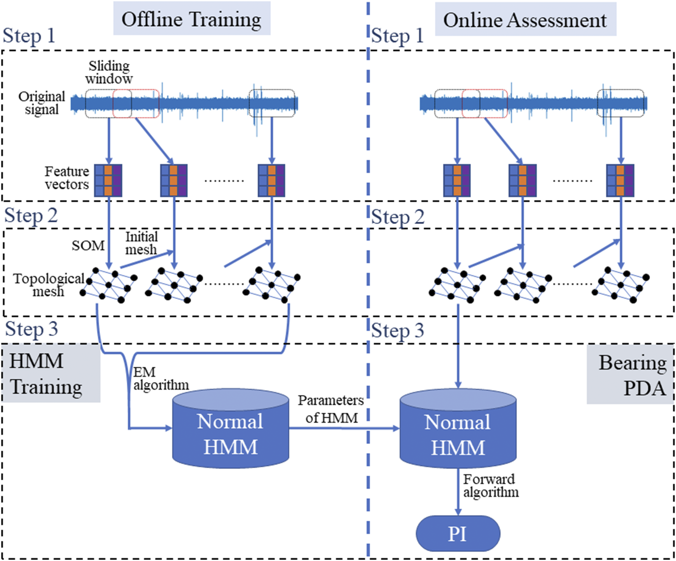

3.1. Offline training stage

Step 1

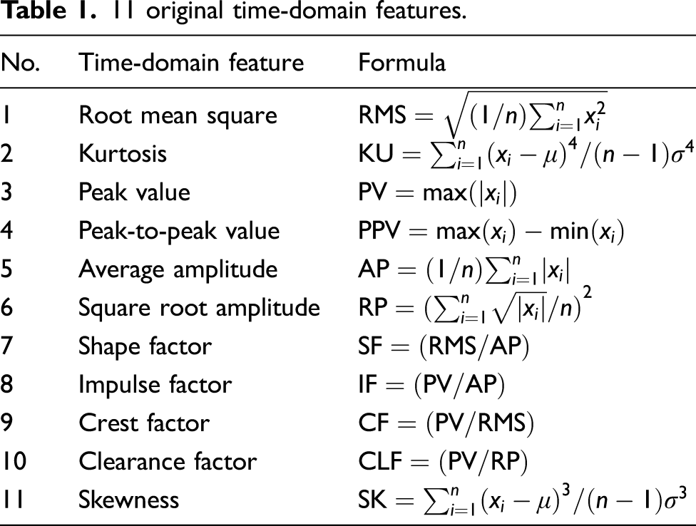
Original feature extraction. In real scenarios, it is usually hard to acquire the failure dataset for offline model training, whereas the normal state data can be obtained easily. So, bearing vibration data under the normal operation state are used as training data. For the purpose of data augmentation, a sliding window is often implemented, with the window size and sliding step determined by the number of training feature instances. Eleven commonly used time-domain features are calculated from normal vibration data, such as RMS, kurtosis (KU), peak value, and so on. These features and their caculation formulas are listed in Table 1, where $x_{i}$ is the discrete time signal, $μ$ and $σ$ denote its mean value and standard deviation separately.

Table 1.

11 original time-domain features.

No.	Time-domain feature	Formula
1	Root mean square	$RMS = \sqrt{(1 / n) \sum_{i = 1}^{n} x_{i}^{2}}$
2	Kurtosis	$KU = \sum_{i = 1}^{n} {(x_{i} - μ)}^{4} / (n - 1) σ^{4}$
3	Peak value	$PV = max (\| x_{i} \|)$
4	Peak-to-peak value	$PPV = \max (x_{i}) - \min (x_{i})$
5	Average amplitude	$AP = (1 / n) \sum_{i = 1}^{n} \| x_{i} \|$
6	Square root amplitude	$RP = {(\sum_{i = 1}^{n} \sqrt{\| x_{i} \|} / n)}^{2}$
7	Shape factor	$SF = (RMS / AP)$
8	Impulse factor	$IF = (PV / AP)$
9	Crest factor	$CF = (PV / RMS)$
10	Clearance factor	$CLF = (PV / RP)$
11	Skewness	$SK = \sum_{i = 1}^{n} {(x_{i} - μ)}^{3} / (n - 1) σ^{3}$

Step 2

Topological representation extraction. To improve the stability of original feature space, the topological representations of original feature vectors are learned by the SOM. As to the determination of the number of map units, both the quantization error (QE) and computational efficiency are considered. The QE is the average distance between the input data vectors and their BMUs, which is usually adopted to validate the mapping quality of the trained SOM. As the number of map units increases, the QE would decrease gradually and then tend to converge. However, high number of map units will increase the computational time. Also, some weight vectors may deviate to the outliers. In this article, a training instance is first pretrained at different map sizes to choose a suitable number of map units.

To obtain ordered weight vectors, weight vectors generated from the previous input feature set is used to initialize the weight vectors in the current training process. By this means, the SOM training process can also be accelerated. After iterative weight updating, a topological mesh is finally formed, which roughly approximates the probability density function of input features. Compared with original feature space, its topological representation is more stable and representative because outliers and random interferences are eliminated, whereas the general distribution of the input feature vectors is preserved. Finally, after topological meshes of all the training feature samples are learned by the SOM, weight vectors of these topological meshes are taken as the degradation features for PDA model establishment.

Step 3

Offline training of the HMM-based assessment model. Weight vectors extracted from vibration signals of bearings under the normal state by following Steps 1 and 2 are taken as the input to train a normal HMM. For every training instance, the input weight vectors can be written as $W = {W_{i}, i = 1,2, \dots, D}$ , where D is the number of map units and $W_{i}$ is weight vector of the ith unit whose dimension equals the number of original features. The parameters of HMM, $λ = (N, M, π, A, B)$ , are estimated by the EM algorithm. It should be noted that the number of hidden states N in the HMM affects its generation performance. Too many hidden states may lead to an overfitting problem. So, in this article, N is prespecified as two according to empirical values (Yu, 2012). After training, a normal HMM is established as the assessment model.

3.2. Online assessment stage

Step 1

Original feature extraction. Just like Step 1 in offline training stage, original time-domain features are extracted from online vibration data.

Step 2

Topological representation extraction. Original features extracted from the online testing data are trained with the SOM. Parameter determination and the SOM training process is the same as the offline training stage. In detail, the topological mesh of the input feature vectors is trained iteratively following the steps in Section 2.1, that is, initialization, competition, cooperation, and adaptation. For every input feature vector, weight vectors extracted from previous testing instance can be used for initialization in the current process to save computational time. Euclidian distances between the input feature vector and all the weight vectors are calculated. After competition, the map unit whose weight vector is closest to the input vector is identified as the BMU. Then, weight vectors of the BMU and its topological neighbors are updated to move closer to the input vector. Finally, after a certain number of iterations, the weight vectors converge to the input vectors, and the topological mesh is formed. Weight vectors of the topological mesh are used as degradation features.

Step 3

Bearing PDA. Degradation features under the current state are fed into the normal HMM $λ$ established in the offline training stage. The input weight vectors for assessment are denoted as $W_{A}$ . Given assessment model $λ$ , the LLP of $W_{A}$ can be calculated using the forward–backward algorithm

L L P = \log (P (W_{A} | λ))

(10)

where LLP indicates how well the input weight vectors follow the probability distribution of the HMM trained by normal bearing data. If the input features are extracted from normal data, then LLP will be around the usual values of normal training data. While the current bearing state deviates from the normal state, LLP tends to be smaller than normal LLPs. Thus, LLP is adopted as the PI. According to the varying trend of LLPs, initial degradation and the commencement of bearing faults can be detected in time, and bearing performance degradation tendency can be evaluated eventually. It should be noted that the LLP indicator can qualitatively indicate the bearing performance degradation tendency and detect the bearing degradation states but cannot directly assess the quantitative degradation degree of the bearing.

4. Experimental verification and analysis

4.1. Experiment 1

4.1.1. PRONOSTIA

PRONOSTIA is an experimentation platform designed and realized by AS2M department of FEMTO-ST Institute (Nectoux et al., 2012). The platform is shown in Figure 2. It is composed of a rotating part, a degradation generation part, and a measurement part. The motor speed is 1800 r/min, and the radial force reduces the bearing’s life duration by setting its value up to the bearing’s maximum dynamic load 4000 N. Bearing 1_1 is the test bearing running from normal to failure. The rotating frequency is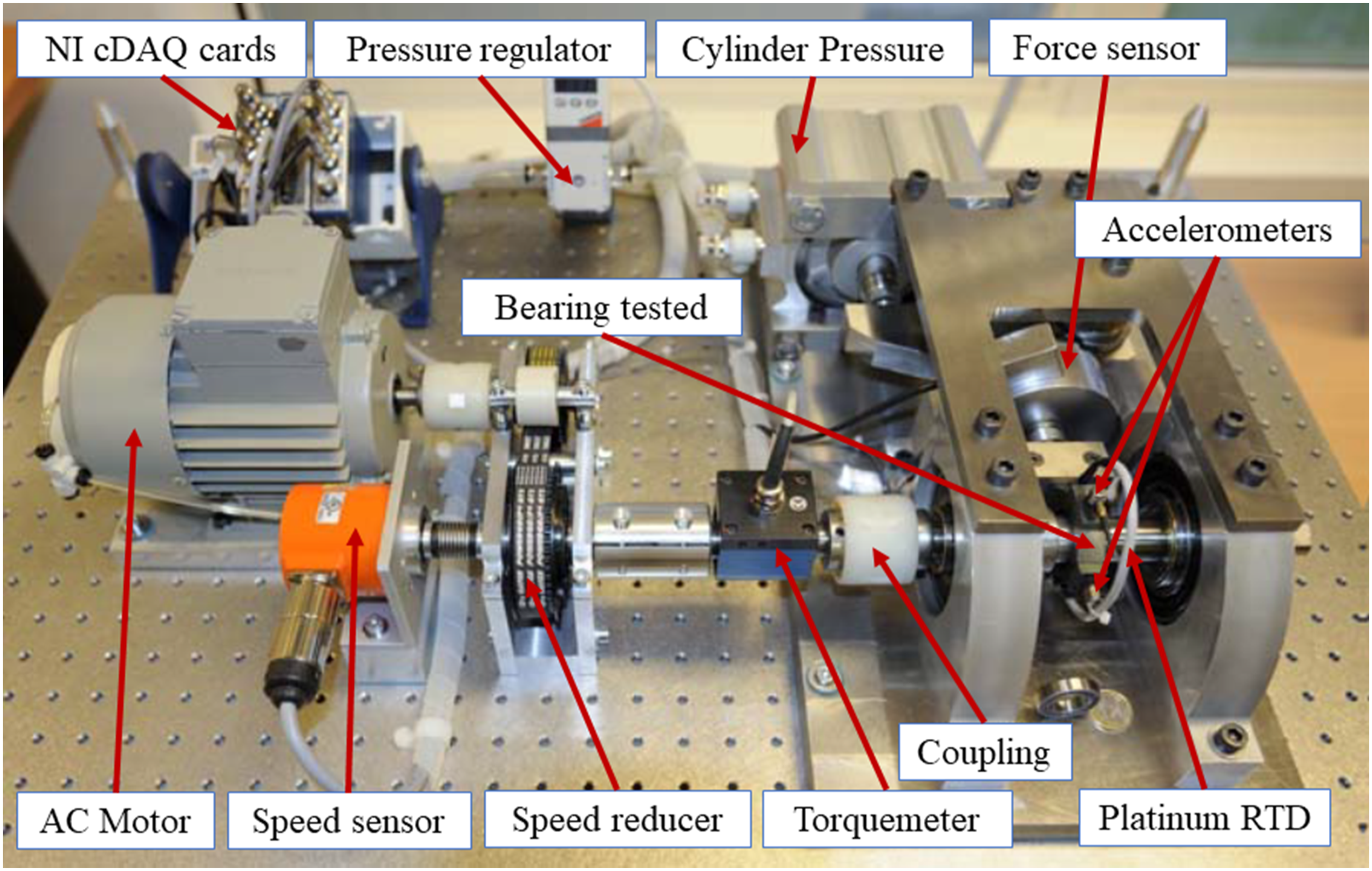 $f_{r}$ = 30 Hz. The sample frequency is 25.6 kHz, and a file of 2560 samples (i.e., 1/10 s) is recorded for every 10 s. 2803 files are recorded during its whole lifetime. The first 500 files which are most probably in the normal stage are adopted as the training dataset. And the total 2803 files in the whole run-to-failure lifetime are used as the test dataset.

4.1.2. Degradation feature extraction based on SOM

Firstly, 11 original time-domain features are extracted from each data file. Every statistical feature is calculated from 128 samples, which means each file generates 20 feature vectors. The time-domain vibration data, the widely used RMS, and kurtosis features of Bearing 1_1 are plotted in Figure 3. The vibration signal in Figure 3(a) increases gradually over time and increases sharply when the bearing approaches the final severe degradation stage. The RMS curve in Figure 3(b) can show the degradation tendency. However, it is difficult to observe the slight degradation stage. Also, there are some subtle fluctuations in the RMS curve. In Figure 3(c), there are a large number of outliers in the kurtosis curve, which may easily lead to false alarms in bearing PDA. Therefore, original time-domain features RMS and kurtosis cannot be directly used as the PI for bearing PDA.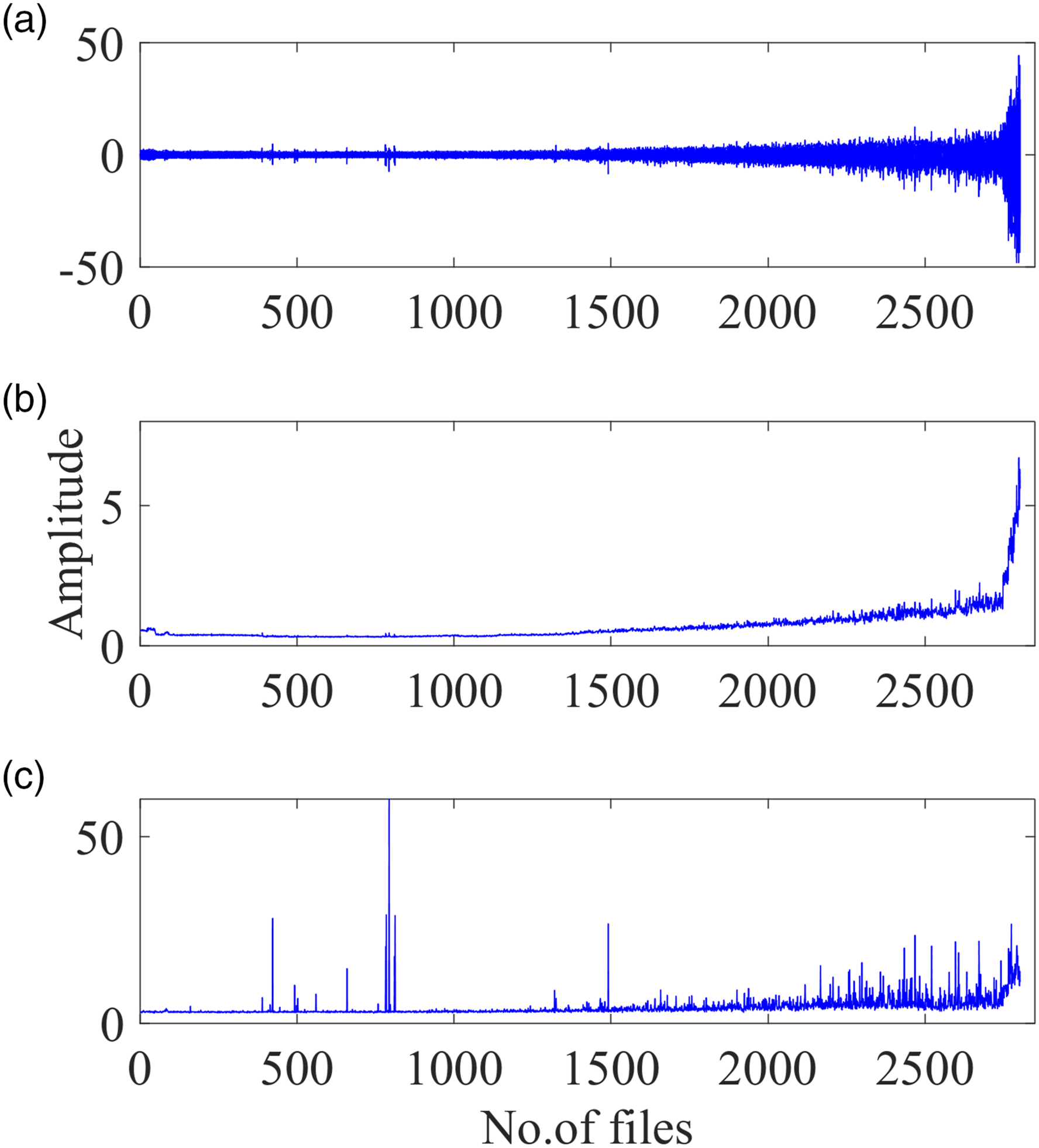

Then, original features of all the 2803 files are grouped by a sliding window with a size of 100 files, and the siding step is 1 file. Consequently, the original features of 2803 files are divided into 2704 feature groups of 2000 feature vectors. Each feature group is trained by the SOM to obtain the topological mesh. To determine the number of map units, the first group of feature vectors is trained with different topological mesh sizes. The mesh size is chosen as $5 \times 5$ to strike a balance between the QE and computational efficiency. Through SOM training, topological meshes are generated from the original features for all the groups. For the convenience of demonstration, some topological meshes obtained by RMS and kurtosis features corresponding to different data files in the degradation process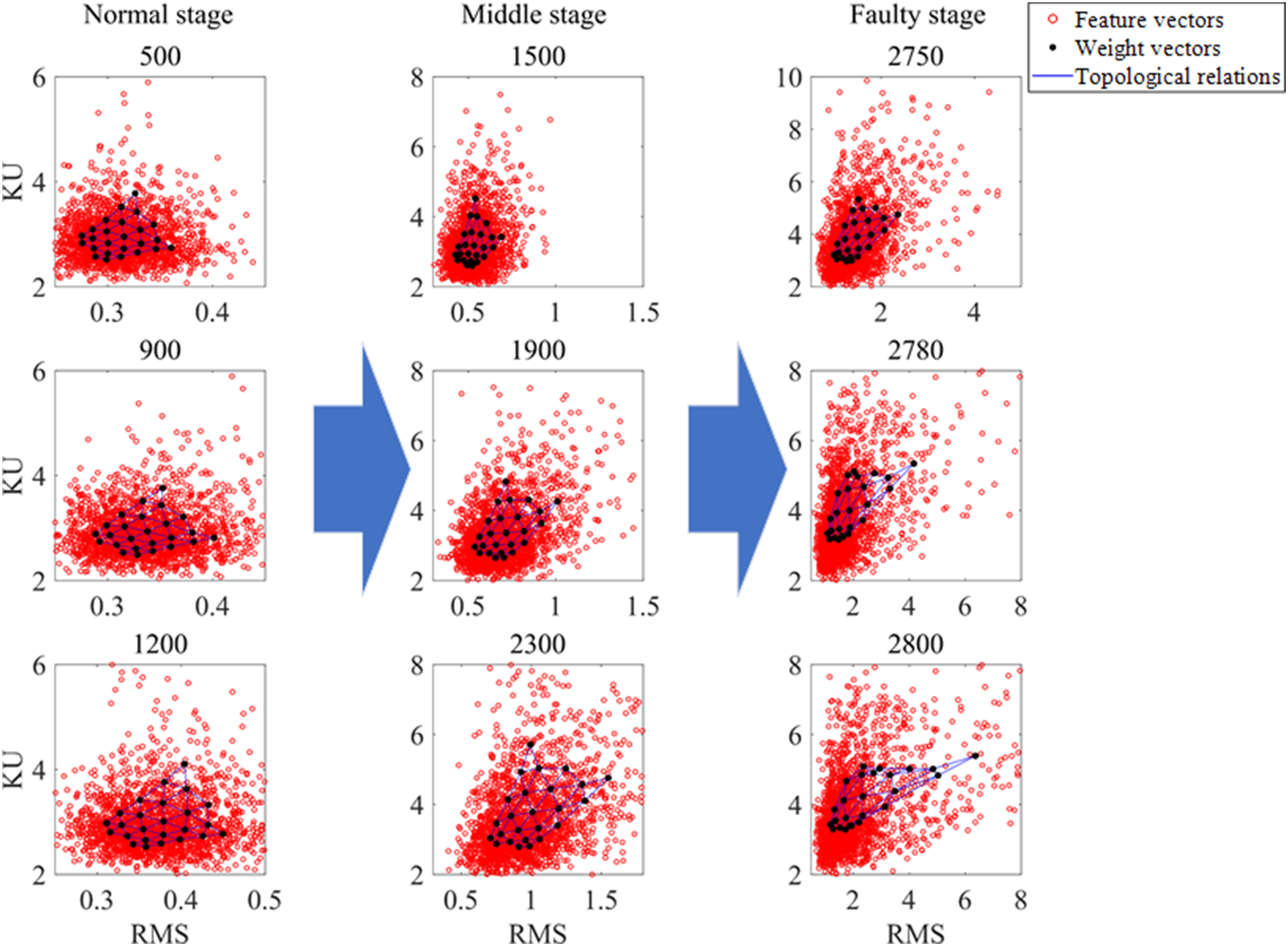 are shown in Figure 4.

As shown in Figure 4, SOM maps original feature vectors into a mesh which preserves the topology of the original features. Units on the mesh are concentrated in the region with high density of feature vectors, and outliers in the feature vectors are hereby removed. Topological meshes in Figure 4 are roughly divided into three groups according to the RMS curve in Figure 3(b). The first group of topological meshes corresponding to the 500th, 900th, and 1200th data files may belong to the normal stage. The last group may belong to the final faulty stage. As shown in Figure 4, the first group of topological meshes are basically similar in the normal stage. Then, from the middle stage to the faulty stage, topological meshes deviate from the normal region gradually. In the last stage, meshes change more rapidly, which indicates that the bearing state is very unstable. So, the topological mesh is stable in the normal stage and sensitive to the change of the bearing states in the degradation process.

4.1.3. Bearing PDA using HMM

Weight vectors of the beginning 500 topological meshes are used to train the normal HMM. Then, the trained normal HMM is used as the assessment model to evaluate the bearing performance. Weight vectors of the topological meshes generated in the whole lifetime are fed into the normal HMM. The LLP output of the normal HMM is chosen as the PI. Finally, the PI curve is shown in Figure 5(a).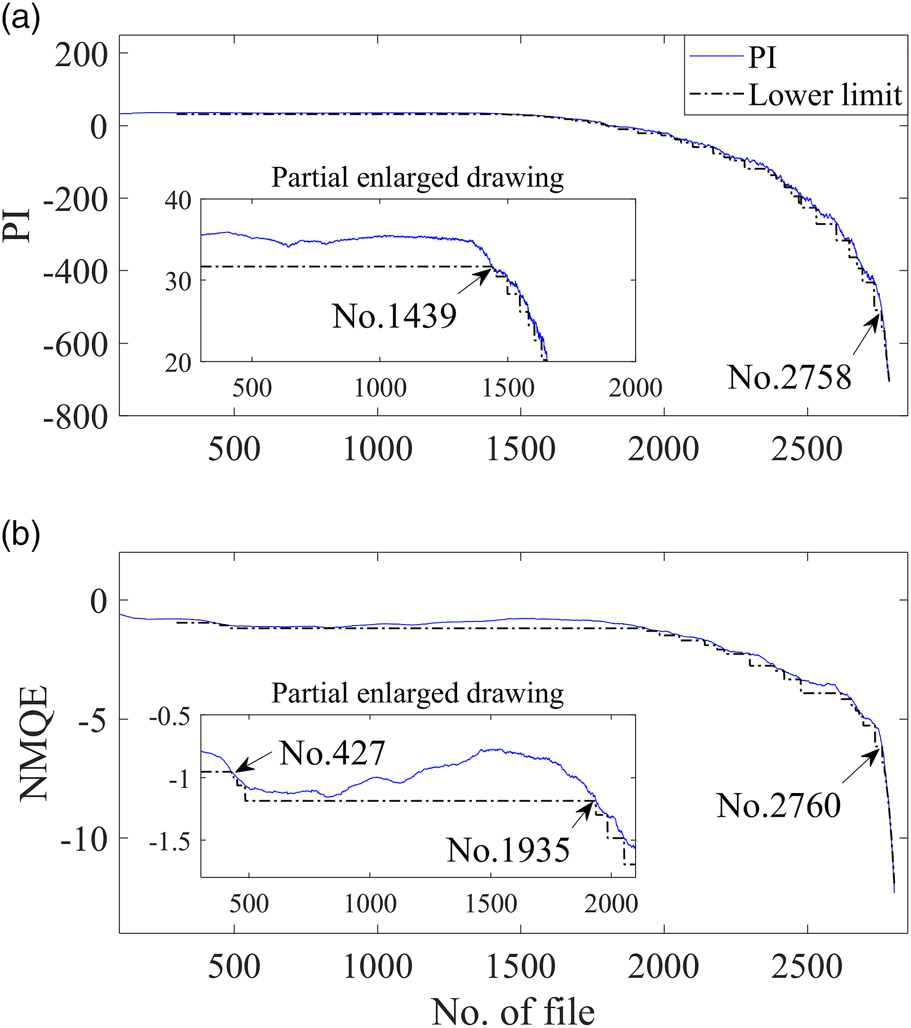

For comparison, a PDA method based on the SOM (Qiu et al., 2003) is implemented. In this method, the MQE is adopted as the PI. Just like the proposed method, the first 500 groups of time-domain feature vectors are used to train the SOM. Then, the whole lifetime feature vectors are fed into the trained SOM, and MQE indicators are calculated for bearing PDA. For the convenience of comparison, negative MQE (NMQE) is adopted here because it has a decreasing trend. The result is shown in Figure 5(b).

In Figure 5, the dotted line is the lower limit of the PI curve, which is calculated by the Laida criterion (also known as $3 σ$ rule). 100 PIs before current PI are taken as historical data. To avoid false alarm, PI threshold is updated until abnormal points appear for 10 times continuously. Consequently, adaptive PI thresholds will be obtained in the PDA process. In Figure 5, both results can reflect the degradation tendency. But the PI curve of the proposed method is more stable in the first 1400 files of the normal stage, whereas the SOM-based method may trigger a false alarm at 427th file. In the proposed method, PI values begin to drop continuously around 1439th file and thus initial degradation can be detected. Then, PI values decrease monotonically, which indicate that the bearing performance deteriorates gradually. Around 2758th file, the PI curve presents a sharp decline, and obvious bearing fault can be detected. So, according to the PI curve and the calculated thresholds, the bearing degradation process can be divided into three stages: normal stage before the 1439th file, early degradation stage between the 1439th file and the 2758th file, and the severe degradation stage after the 2758th file until final failure. This conclusion is consistent with the analysis results of time waveform and RMS indicators in Figure 3. Anyway, it is obviously more accurate and reliable.

To verify the above results, envelope spectrum analysis is performed at the two changing points, that is, 1439th and 2758th files. Time waveforms and envelope spectrums of these two files are shown in Figure 6. In Figure 6(a), some weak impacts can be found in the time waveform. There are some impacts, but the fault characteristic is not obvious in Figure 6(c). So, incipient degradation is supposed to commence after 1439th file. By contrast, in Figure 6(b), stronger impacts can be observed. Meanwhile, some obvious peaks can be detected at fault characteristic frequency $f_{b} = 215 Hz$ and $2 f_{b}$ in the envelope spectrum. So, bearing damage has occurred and developed in the 2758th file.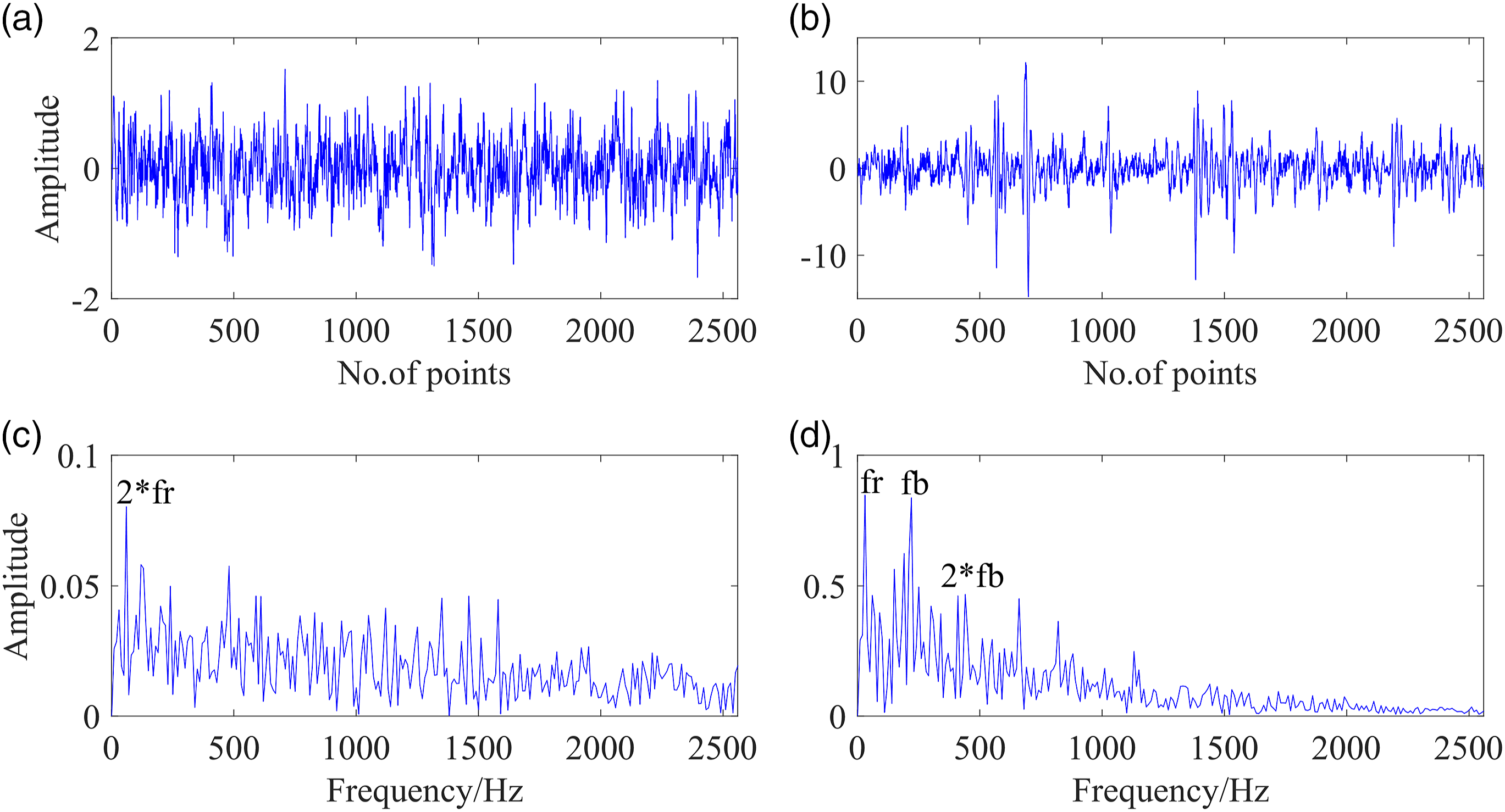

As to the computational time, in the online assessment stage, the average training time for the SOM to train each group of weight vectors is 0.1062 s. And the total time for calculating each PI is about 0.1157 s. The proposed method is executed with MATLAB software in a computer with Intel Core i7-4710HQ (2.50G Hz) CPU, 16 GB memory. It can meet the requirement of online application in most cases.

4.2. Experiment 2

4.2.1. Experimental setup

To further validate the effectiveness and superiority of the proposed method, an accelerated bearing life experiment was conducted in Hangzhou Bearing Test & Research Center (HBRC). The test rig (ABLT-1A) is shown in Figure 7(a). The motor speed was 3000 r/min. A load of 12.744 kN was applied on the bearings to accelerate the bearing to failure. Vibration signals were acquired by three PCB348 A acceleration sensors, one anti-aliasing filter, and a data acquisition card NI PCI-6023E. The load and sensor installation sketch are shown in Figure 7(b) and 7(c). The data sampling frequency was 25.6 kHz. 20,480 samples (0.8 s) were acquired every minute. In this experiment, bearing B1 in Figure 7(b) ran to failure first. So, this bearing was chosen to be analyzed. After testing, large areas of pitting were found in the inner race of a final damaged bearing B1, which is shown in Figure 7(d).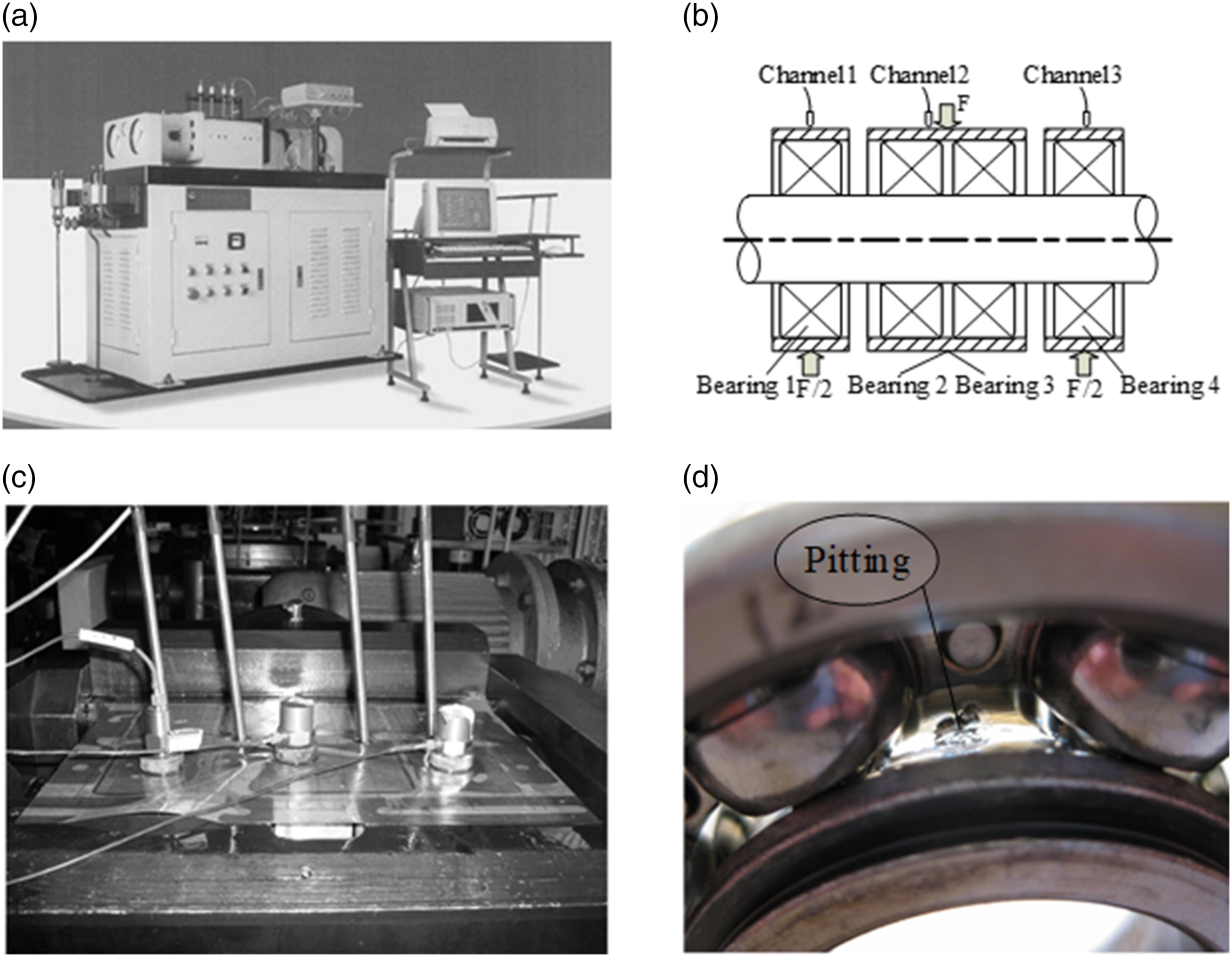

The whole life of bearing 1 is 2469 min. Vibration data in the beginning 500 min are most probably in the normal stage and thus are adopted as the training dataset. The 2469 min whole lifetime data are used as the test dataset.

4.2.2. Degradation feature extraction

The time-domain waveform, RMS, and kurtosis curves of the vibration signal in whole lifetime are shown in Figure 8. In general, the normal stage and faulty stage can be observed in these curves. However, the incipient degradation is difficult to detect. Meanwhile, there are some outliers and fluctuations in RMS and kurtosis, which may affect PDA results.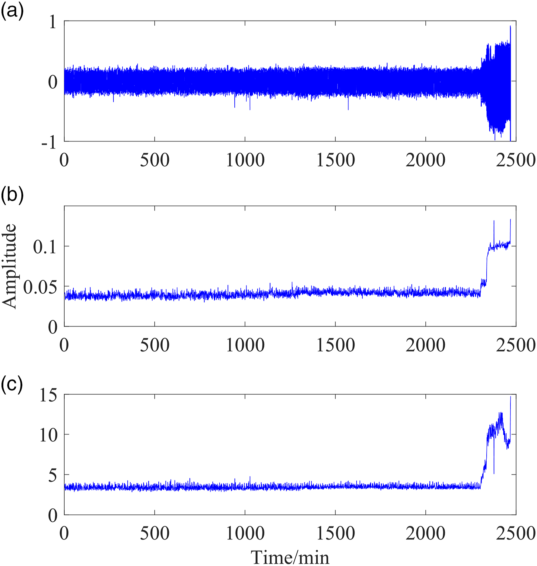

The process of degradation feature extraction is just like the previous experiment. The vibration signal is divided into 2460 groups containing 20,480 samples through a sliding window. The window size is 10 min, and the sliding step size is one minute. First, 11 time-domain features are extracted from each 128 samples of the vibration data.

Then, the SOM is applied to extract the topological representation of the original feature space. The size of topological mesh is selected as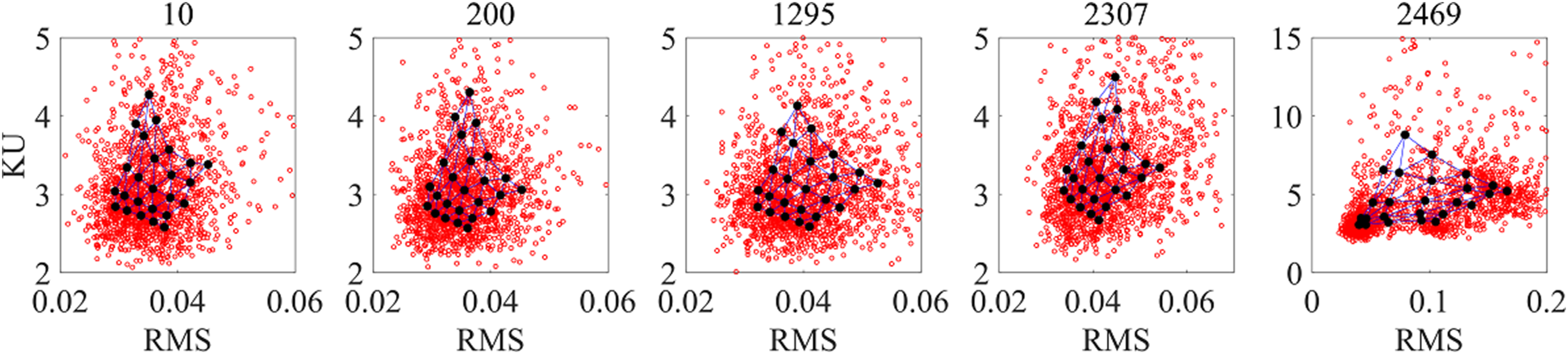 $5 \times 5$ . Some topological meshes obtained from RMS and kurtosis features are drawn in Figure 9. Similarly, it can be found that outliers in the original feature space is eliminated in the topological mesh. The topological meshes are stable in the normal stage (the 10th and 200th min). Whereas from the 1295 min to the 2469 min, the topological meshes deviate from the normal region. So, topological representations are more robust and representative than original features. In this experiment, it takes about 0.0608 s to extract every mesh.

4.2.3. Bearing PDA using HMM

Weight vectors of first 500 meshes are used to train the normal HMM. Then, taking all the degradation features in the whole life as input of the trained normal HMM, the PI can be obtained and plotted in Figure 10(a). In addition, the SOM-based PDA is implemented for comparison, whose PDA result is shown in Figure 10(b).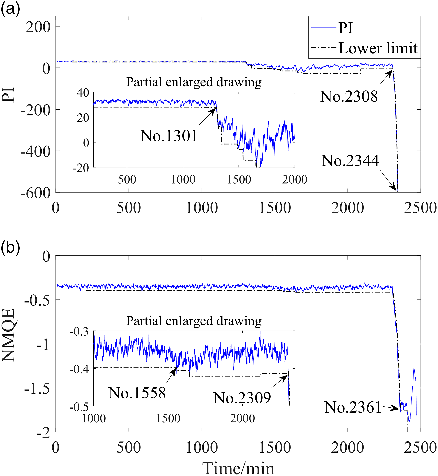

In Figure 10(a), the PI curve remains steady in the beginning of the normal stage. Then, around 1301 min, the PI begins to decline and then remains at low levels. This indicates the probability distribution of vibration data after 1301 min is much different from normal state data. Initial degradation is detected at 1301 min. Around 2308 min, the PI drops sharply and decreases to negative infinity after 2344 min. Therefore, according to the proposed method, 0–1301 min, 1301–2308 min, and 2308–2469 min can be identified as the normal stage, early degradation stage, and severe faulty stage, respectively. By contrast, in Figure 10(b), there are obvious fluctuations in the NMQE curve in the normal stage. The beginning time of early degradation stage 1558 min is much latter. And the overall tendency is not monotonous. The PI curve drops sharply from 2309 min, but after 2361 min, it fluctuates greatly, which is inconsistent with the irreversible degradation process. So, the proposed method outperforms the SOM-based method.

To verify the effectiveness of the proposed method, envelope spectrum analysis is carried out. In this experiment, the rotating frequency is $f_{r} = 50 Hz$ , and characteristic frequency of inner race fault is $f_{i} = 246 Hz$ . Time waveforms and envelope spectrums at two changing points1301 and 2308 min are shown in Figure 11. At 1301 min, there are some impacts in Figure 11(a). Meanwhile, peaks at fault characteristic frequencies $f_{r}$ and $f_{i}$ can be found in envelope spectrum, but they are not dominant, which indicate bearing incipient defect. So, initial degradation may occur from 1301 min. At 2308 min, obvious periodic impacts in time waveform and clear components at characteristic frequency $f_{i}$ and its side frequencies in the envelope spectrum $f_{i} \pm f_{r}$ indicate that the bearing has inner race fault. This conclusion is also proved by the actual failure photo in Figure 7(d). These results verify the effectiveness of the PDA results.

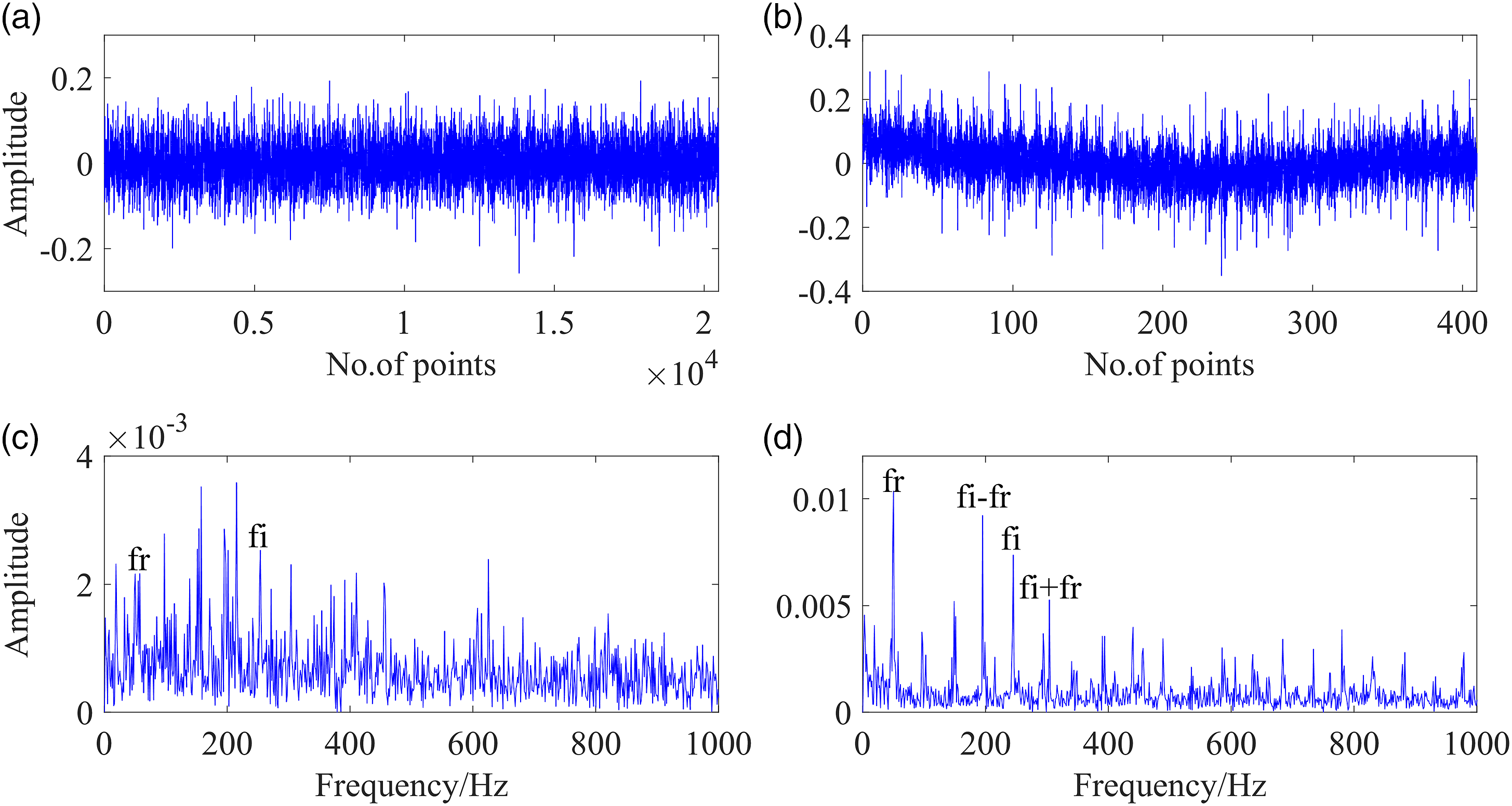
Furthermore, the proposed method is compared with existing HMM-based PDA methods. In the conventional HMM-based method, 11 time-domain features are directly used as degradation features and fed into the HMM. In other methods, PCA, KPCA, and LPP are adopted to reduce the feature dimension, respectively, and then fed them into the HMM. PDA results are shown in Figure 12. As shown in Figure 12, there are obvious fluctuations in the PI curves of these four existing PDA methods. Moreover, just the normal stage and the severe faulty stage can be observed. These comparisons further validate the superiority of the proposed method.

To summarize, the identification results of bearing degradation stages obtained by the proposed PDA method and all the above comparative methods are listed in Table 2. It clearly shows that among these methods, only the proposed method can detect the initial degradation a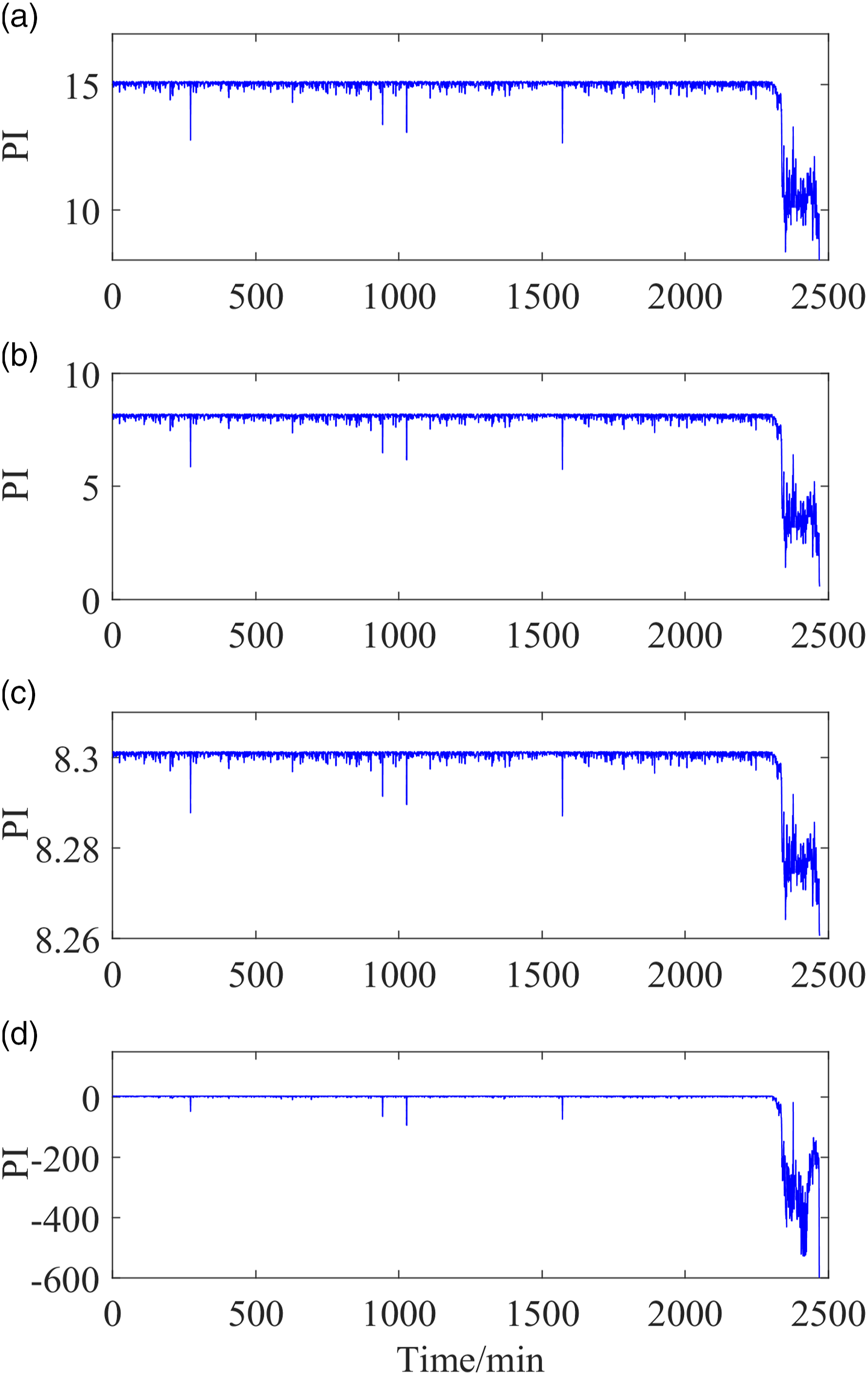nd evaluate three degradation stages in the bearing’s whole lifetime correctly.

Table 2.

Comparison results of different performance degradation assessment methods.

Method	Normal stage/min	Initial degradation stage/min	Severe faulty stage/min
Proposed method	0–1301	1301–2308	2308–2469
SOM	0–2309	Not found	2309–2469
Conventional HMM	0–2334	Not found	2334–2469
PCA–HMM	0–2334	Not found	2334–2469
KPCA–HMM	0–2334	Not found	2334–2469
LPP–HMM	0–2334	Not found	2334–2469

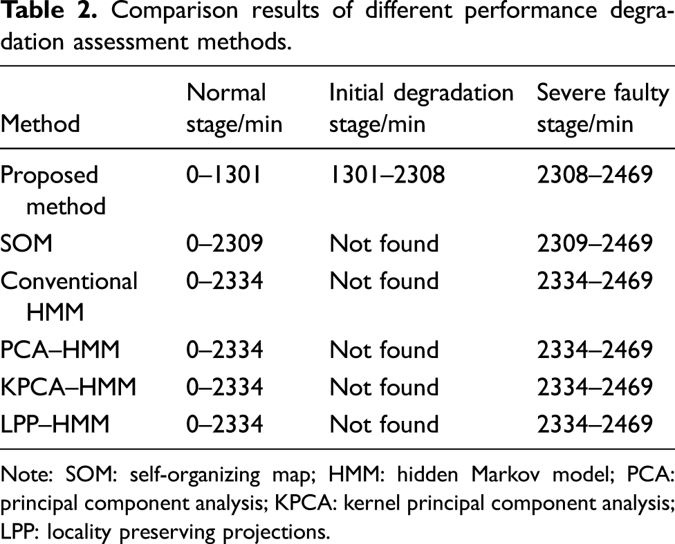
Note: SOM: self-organizing map; HMM: hidden Markov model; PCA: principal component analysis; KPCA: kernel principal component analysis; LPP: locality preserving projections.

5. Conclusions

In this study, a new bearing PDA method based on the topological representation and HMM is proposed. The topological meshes obtained by the SOM can represent the general distribution of original feature vectors and hereby eliminate the influences of outliers and some interferences in the vibration signals. Through the combination of topological representation and HMM, more robust and accurate bearing PDA results can be obtained. Two different experimental datasets are used to verify its effectiveness, and comparisons with SOM-based method, conventional HMM, PCA–HMM, KPCA–HMM, and LPP–HMM methods further prove its superiority.

Results show that the PI curve of the proposed method is more stable in normal stage and presents a monotonic decreasing trend in the continuous degradation process. This robust property of the proposed PI will facilitate a reliable bearing performance assessment. Moreover, it is more sensitive to the change of bearing degradation states. Initial degradation at 1439th file in Experiment 1 and 1301 min in Experiment 2 can be identified, whereas comparative methods cannot. According to the PI thresholds, the bearing degradation process in Experiment 1 is divided into three stages: 0–1439, 1439–2758, and 2758–2803 files. In Experiment 2, they are 0–1301, 1301–2308, and 2308–2469 min. In conclusion, the proposed method can enhance the robustness and accuracy of the bearing PDA results. However, how to assess the quantative degradation degree is still a challenging problem in bearing PDA, and further research needs to be carried out on it in the future.

Footnotes

Declaration of conflicting interests

The author(s) declared no potential conflicts of interest with respect to the research, authorship, and/or publication of this article.

Funding

The author(s) disclosed receipt of the following financial support for the research, authorship, and/or publication of this article: This work was supported by the National Natural Science Foundation of China (grant no. 51505277).

ORCID iDs

Ran Wang

Jihao Jin

References

Cerrada

Sánchez

R-V

, et al. (2018) A review on data-driven fault severity assessment in rolling bearings. Mechanical Systems and Signal Processing 99: 169–196.

Cong

Chen

Dong

, et al. (2013) Short-time matrix series based singular value decomposition for rolling bearing fault diagnosis. Mechanical Systems and Signal Processing 34(1–2): 218–230.

Dong

Luo

(2013) Bearing degradation process prediction based on the PCA and optimized LS-SVM model. Measurement 46(9): 3143–3152.

Hong

Zhou

Zio

, et al. (2014) Condition assessment for the performance degradation of bearing based on a combinatorial feature extraction method. Digital Signal Processing 27: 159–166.

Jiang

Chen

Dong

. (2016) Hidden Markov model and nuisance attribute projection based bearing performance degradation assessment. Mechanical Systems and Signal Processing 72–73: 184–205.

Jiang

Chen

Dong

, et al. (2017) An intelligent performance degradation assessment method for bearings. Journal of Vibration and Control 23(18): 3023–3040.

Kohonen

(1990) The self-organizing map. Proceedings of the IEEE 78(9): 1464–1480.

Lei

Guo

, et al. (2018) Machinery health prognostics: a systematic review from data acquisition to RUL prediction. Mechanical Systems and Signal Processing. 104: 799–834.

Liu

Chen

Dong

(2015) Singular spectrum analysis and continuous hidden Markov model for rolling element bearing fault diagnosis. Journal of Vibration and Control 21(8): 1506–1521.

10.

Nectoux

Gouriveau

Medjaher

, et al. (2012) PRONOSTIA: an experimental platform for bearings accelerated degradation tests. In: IEEE international conference on prognostics and health management, PHM’12, Denver, Colorado, 08–10 June 2012, pp. 1–8. USA: IEEE.

11.

Ocak

Loparo

Discenzo

(2007) Online tracking of bearing wear using wavelet packet decomposition and probabilistic modeling: a method for bearing prognostics. Journal of Sound and Vibration 302(4–5): 951–961.

12.

Pan

Hong

Chen

, et al. (2019) Performance degradation assessment of a wind turbine gearbox based on multi-sensor data fusion. Mechanism and Machine Theory 137: 509–526.

13.

Qiu

Lee

Lin

, et al. (2003) Robust performance degradation assessment methods for enhanced rolling element bearing prognostics. Advanced Engineering Informatics 17(3–4): 127–140.

14.

Rabiner

(1989) A tutorial on hidden Markov models and selected applications in speech recognition. Proceedings of the IEEE 77(2): 257–286.

15.

Rai

Upadhyay

(2016) A review on signal processing techniques utilized in the fault diagnosis of rolling element bearings. Tribology International 96: 289–306.

16.

Randall

Antoni

(2011) Rolling element bearing diagnostics–a tutorial. Mechanical Systems and Signal Processing 25(2): 485–520.

17.

Wang

Sun

(2019) The application of matching pursuit based on multi feature pattern set in the signal processing of rotating machinery. Journal of Vibration and Control 25(13): 1974–1987.

18.

Wang

, et al. (2018) An intelligent fault diagnosis method of rolling element bearing based on acoustic imaging and gabor wavelet transform. In: 25th international congress on sound and vibration 2018: Hiroshima calling, ICSV 2018, Hiroshima, Japan, 8–12 July 2018, pp. 2684–2691. USA: IIAV.

19.

Wang

Chen

Wang

, et al. (2019) Degradation evaluation of slewing bearing using HMM and improved GRU. Measurement 146: 385–395.

20.

(2012) Health condition monitoring of machines based on hidden markov model and contribution analysis. IEEE Transactions on Instrumentation and Measurement 61(8): 2200–2211.

21.

J-B

(2011) Bearing performance degradation assessment using locality preserving projections. Expert Systems with Applications 38(6): 7440–7450.