Improving model-based compensation method for real-time hybrid simulation considering error of identified model

Abstract

Time delay is a critical and unavoidable problem in real-time hybrid simulation. An accurate and effective compensation method for time delay is necessary for the safety of real-time hybrid simulation and the reliability of test results. Generally, a model-based compensation method can be adopted, which is derived from the identified transfer function by assuming the latter can accurately represent the real plant. However, there must be some differences between the transfer function and the real plant. To facilitate the development of real-time hybrid simulation, we proposed a two-stage feedforward compensation method considering the error between the transfer function identified and the real plant. The compensation strategy proposed in this study was not only based on the transfer function but also introduced an error model as a second-stage compensation into a compensator to realize the synchronization of command and measurement. To verify the efficiency of the proposed method, comparisons in time domain and frequency domain with the feedforward compensator in a model-based feedforward–feedback control method were carried out. Compared with the feedforward compensator, the two-stage method achieved better tracking performance, especially in the high-frequency bandwidth. The test results verified that for a band-limited white noise of 0–30 Hz, the phase lag of the actuation system can be limited to ±5°. Finally, the two-stage method was applied to a real-time hybrid simulation of a two-story frame to illustrate its compensation effect on time delay.

Keywords

Real-time hybrid simulation time-delay compensation model-based feedforward and feedback control identified plant error

Highlights

This article proposed a two-stage time-delay compensation method for real-time hybrid simulation (RTHS) by introducing the error model as the second-stage compensation into the model-based feedforward (FF) compensation method proposed by Phillips et al. (2012a, 2012b).

Compared with the FF compensator, the two-stage compensation method achieved a better tracking performance, especially at the high-frequency bandwidth.

The performance of the two-stage method was confirmed by experimental results in time domain and frequency domain to indicate the improvement of the compensation effect.

The proposed method is applied to an RTHS for a two-story frame to verify its efficiency of time-delay compensation.

1. Introduction

Real-time hybrid simulation (RTHS) is a powerful experimental method for investigating the behaviors of structures under dynamic loads. In RTHS, the component with clear constitutive relationships is modeled as a numerical substructure (NS), and the other component, which responds to the loading rate and/or is difficult to simulate, is treated as a physical substructure (PS). The synchronization of the interface(s) between the NS and PS is realized via loading devices and sensors. Consequently, the displacements calculated by the NS are applied to the PS by loading devices, and the feedback forces of the PS are fed back to the NS through sensors for the next calculation time step.

In recent years, a significant effort has been focused on RTHS test methods. Chen et al. (2009) investigated the stability of, and presented the implementation of, the Chen and Ricles integration algorithm in RTHS. Shao et al. (2010) revealed an RTHS method with PSs excited by shaking tables and auxiliary actuators. Schellenberg et al. (2013) investigated the shaking table hybrid simulation method for testing midlevel seismic isolation systems. For educational and research purpose, an RTHS to investigate the dynamic behavior of a tuned liquid damper (TLD) structure system is implemented with a shake table (Ashasi-Sorkhabi et al., 2015; Malekghasemi et al., 2015). Wang et al. (2016) researched the RTHS of multistory structures installed with the TLD. Zhang et al. (2017) investigated the performance of buildings with interstory isolation by shaking table RTHS techniques.

To achieve a successful RTHS, the synchronization of the interface(s) must be guaranteed in real time. Therefore, the displacement calculated must be accurately applied to the PS in real time. At the same time, the reaction response must be immediately fed back to the NS for the next calculation time step. This synchronization not only imposes a high requirement on loading devices but also requires a compensation algorithm to compensate for the displacement calculated. Without effective compensation, time delays would cause inaccurate testing results and even system instability (Horiuchi et al., 1999).

Generally, time-delay compensation methods can be broadly divided into three categories: error-based, record-based, and model-based methods. First, the so-called error-based method compensates the command by comparing the target with the measured response to achieve synchronization on the interface(s) in RTHS. For instance, Darby et al. (2002) proposed an online delay estimation method to calculate the time delay. In the phase lead compensation (Zhao et al., 2003), velocity feedback compensation with phase adjustment is used to compensate the command signal. Chen and Ricles (2009) combined the inverse compensation method and the actuator control error as a secondary compensation to form a dual compensation scheme. Chen and Ricles (2010) developed an adaptive control law using an error tracking indicator to adapt a compensation parameter and conducted an RTHS test (Chen and Ricles, 2012) of a steel frame with a large-scale magneto-rheological damper. Furthermore, a novel integrated compensation method (Liu et al., 2013), which combined model-based and time-delay online estimation methods, was proposed. A new tracking error compensation strategy (Mirza Hessabi et al., 2016) adopting frequency domain–based error indicators was proposed. Combining the polynomial extrapolation (Horiuchi et al., 1999) and the inverse compensation method (Chen, 2007) with Darby’s online delay estimation method (Darby et al., 2002), Li et al. (2019a, 2019b) proposed two adaptive time delay compensation methods with experimental verification. However, the effectiveness of the error-based method is affected by noise and disturbance in the feedback signal. Moreover, this method adjusts the command when there is a difference between the command and the actual measured response, so it is still a delay regulation. It has good compensation performance for low-frequency components in the command signal, but it is not satisfactory for high-frequency components.

Second, the record-based compensation method tries to predict subsequent displacement according to historical records to compensate for time delays. A polynomial extrapolation method was proposed Horiuchi et al. (1999) to predict the actuator displacement. The efficiency of the extrapolation procedure was demonstrated through a series of real-time tests on models considered to be single-degree-of-freedom structures (Nakashima and Masaoka 1999). Horiuchi and Konno (2001) introduced a new method in which the acceleration was linearly predicted and used to calculate the displacement. Wallace et al. (2005) proposed an adaptive forward prediction compensation method to perform a multi-actuator RTHS. The adaptive time series compensator Chae et al. (2013) developed continuously updates the coefficients of the system transfer function during RTHS. The forward prediction adaptive polynomial-based algorithm was combined with the equivalent force control method to improve the accuracy and stability of RTHS (Zhou et al., 2017). To the authors’ knowledge, the effectiveness of record-based compensation methods depends largely on the prediction algorithm used. And it is impossible to predict the command perfectly, which is the main source of error in such methods.

Finally, in the model-based compensation methods, the transfer function model of a plant is constructed, and its inverse is used to compensate for time delays. Chen (2007) proposed a first-order actuator model in the z-domain and used its inverse model as a compensator. A model-based compensation strategy Carrion et al. (2007) was proposed, which considers the dynamics of the servo-hydraulic equipment in a wide frequency range. In this strategy, the feedforward (FF) controller was realized by inverting the transfer function in series with a low-pass filter to render the controller proper. Phillips et al. (2012a, 2012b) further improved this model-based compensation strategy by using displacement and its several high-order derivatives with respect to time to render the FF controller causal and proper. Phillips et al. (2014) extended this model-based compensation strategy to a multi-metric shaking table control strategy. Chen et al. (2015) further developed the model-based compensation method by applying an adaptive control scheme to the feedforward–feedback (FF–FB) controller. Hayati and Song (2016) proposed a discrete-time compensation method that allows the actuator to track inputs with higher frequency content. An infinite impulse response compensation technique (Stehman and Nakata 2016), which can handle the complex magnitude and phase characteristics caused by the control–structure interaction effect, was proposed. The extended Kalman filter–based adaptive compensator (Strano and Terzo, 2016), instead of the fixed-value parameters, was used to identify the model; the extended Kalman filter estimates the parameters continuously, thereby realizing a more versatile model-based approach. Fermandois Cornejo et al. (2018) proposed a model-based control method with a multi-axial RTHS framework. Therefore, as a general method, the model-based strategy can quickly reveal the dynamic characteristic of the prototype model and has been widely used in many fields (Fermandois Cornejo et al., 2018).

Previous studies shown that the major issue of the model-based compensation strategy lies in obtaining the inverse of a real plant. This inverse is then used to compensate for the target displacement. The compensated command is sent to the plant to achieve interface(s) synchronization. Therefore, the key is to determine the exact transfer function that reflects the plant’s characteristics. However, there must be some differences between the transfer function and the real plant. On the one hand, these differences are caused by the assumption that the nonlinear system is linear. On the other hand, the data obtained and used in the identification process have uncertain noise and disturbance, and the identification method itself will also cause errors.

To further improve the performance of the model-based compensation strategy for RTHS, a two-stage compensation strategy is proposed in this study. In this strategy, the inverse of a real plant is constructed more accurately by considering the error between the transfer function identified and the real plant. For the convenience of readers, this article is organized as follows. First, the theoretical derivation of the two-stage method is introduced. Second, an application of the two-stage method is introduced through an experimental procedure. Third, an evaluation of the two-stage method is carried out in the time and frequency domains. Finally, the two-stage method is applied to an RTHS to verify its efficiency.

2. Two-stage FF method

This section details the proposed process of the new two-stage method. For convenience, the identified transfer function is denoted as $G_{I D} (s)$ , the transfer function of the real plant is denoted as $G_{R P} (s)$ , which is assumed to be completely equivalent to the real plant, and the error between $G_{I D} (s)$ and $G_{R P} (s)$ is denoted as $G_{M E} (s)$ .

Then, the following relationship is obtained

G_{M E} (s) = G_{R P} (s) - G_{I D} (s)

(1)

When the displacement command is compensated for only by the FF controller in the model-based FF–FB control method, the relationship between the input command and measured displacement is

\frac{Meas (s)}{Cmd (s)} = \frac{1}{G_{I D} (s)} \cdot G_{R P} (s)

(2)

where

Meas (s)

is the measured displacement of the real plant and

Cmd (s)

is the command displacement.

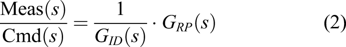
Inserting equation (1) into (2) yields

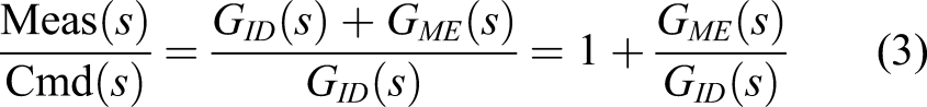
\frac{Meas (s)}{Cmd (s)} = \frac{G_{I D} (s) + G_{M E} (s)}{G_{I D} (s)} = 1 + \frac{G_{M E} (s)}{G_{I D} (s)}

(3)

Thus

Meas (s) = (1 + \frac{G_{M E} (s)}{G_{I D} (s)}) \cdot Cmd (s)

(4)

Expanding equation (4)

G_{M E} (s) = \frac{Meas (s) - Cmd (s)}{1 / G_{I D} (s) \cdot Cmd (s)}

(5)

where

1 / G_{I D} (s)

is the inverse of the identified transfer function,

G_{I D} (s)

. According to the FF–FB method mentioned, it can be rewritten as

G_{FF} (s)

G_{M E} (s) = \frac{Meas (s) - Cmd (s)}{G_{FF} (s) \cdot Cmd (s)}

(6)

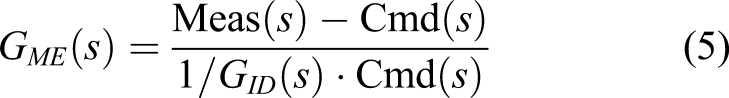
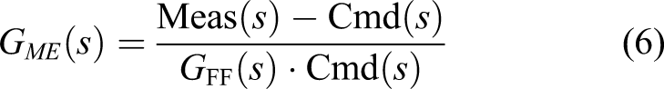
According to equation (6), $G_{M E} (s)$ can be identified using the experimental data. The input of $G_{M E} (s)$ is the command signal compensated by the FF compensator, and the output is the tracking error between the measured displacement and the command signal. However, through multiple trials, the transfer function of $G_{M E} (s)$ cannot be obtained directly via model identification. Therefore, a method was proposed to solve this problem. For completeness and continuity, the method and process of obtaining $G_{M E} (s)$ is described in Section 3.

After $G_{M E} (s)$ is obtained, let the system input command be equation (7)

Cmd (s) = Target (s) - Target (s) \cdot \frac{G_{M E} (s)}{G_{I D} (s)}

(7)

where

Target (s)

is the target displacement that the users want to track.

Then, substituting equation (7) into (4) yields

Meas (s) = (1 + \frac{G_{M E} (s)}{G_{I D} (s)}) \cdot (Target (s) - Target (s) \cdot \frac{G_{M E} (s)}{G_{I D} (s)})

(8)

After simplification

Meas (s) = Target (s) - Target (s) \cdot G_{M E}^{2} (s) \cdot G_{FF}^{2} (s)

(9)

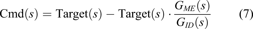
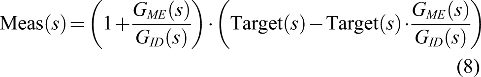
It is found that $G_{M E} (s)$ has a response of small magnitude during the experiment in the frequency domain. As a result, the last term in equation (9) can be completely negligible. This point will be proven in Section 3.

Thus, the equality between the input command and output measurement is achieved

Meas (s) = Target (s)

(10)

In this way, the output of the plant is consistent with the target displacement. The block diagram of the two-stage method is shown in Figure 1.

Figure 1.

Block diagram of two-stage compensate method.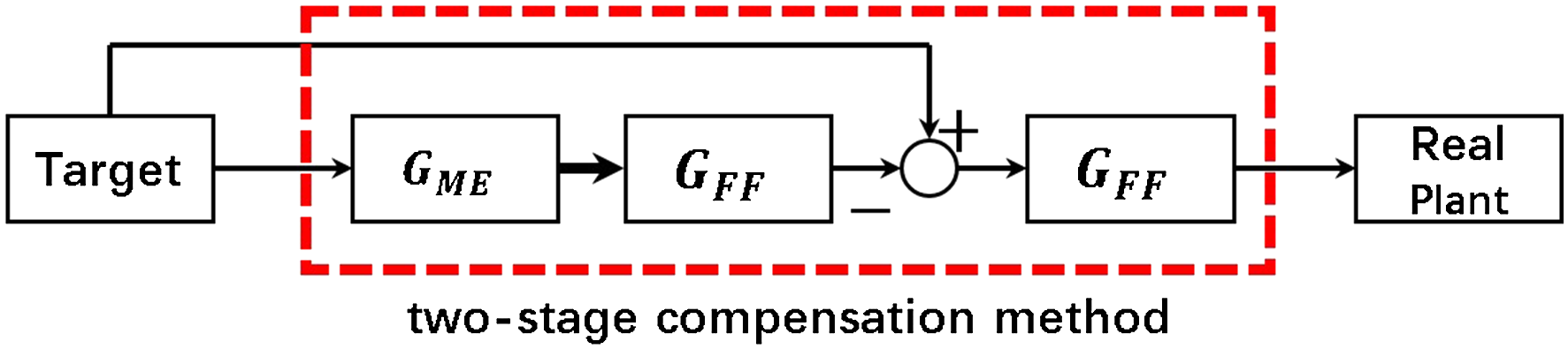

The difference between the model identified and the real plant has previously not been considered in the general model-based compensation method. In the present study, the performance of the model-based FF compensator is further improved by considering this difference. The experimental results in Section 4 show that the compensation effect of the two-stage method is better than that of the model-based FF compensator without considering the model error, $G_{M E} (s)$ , especially in the high-frequency bandwidth.

3. Identification procedure of $G_{ME} (s)$

To illustrate the identification process of $G_{M E} (s)$ and prove that this transfer function can indeed be obtained through experimental data, the identification process is explained using the real-time substructure test system of the Key Laboratory of Coast Civil Structures Safety of Ministry of Education, Tianjin University.

3.1. Experimental setup

The test facility was an MTS servo-hydraulic system (including a FlexTest 60 controller, 244.41s actuator (Figure 2), 340 L/min servo valve, and 600 L/min hydraulic power unit on 3000 psi). One can find more detailed information about the hydraulic servo system in the manuals provided by MTS company’s official Web site. SpeedGoat was used to calculate the compensated command and interact with the MTS controller in real time. SpeedGoat is a powerful real-time computing and processing machine, which is widely used in rapid control prototyping and hardware-in-the-loop simulation. One also can find details about SpeedGoat on its official Web site.

Figure 2.

MTS 244.41s actuator.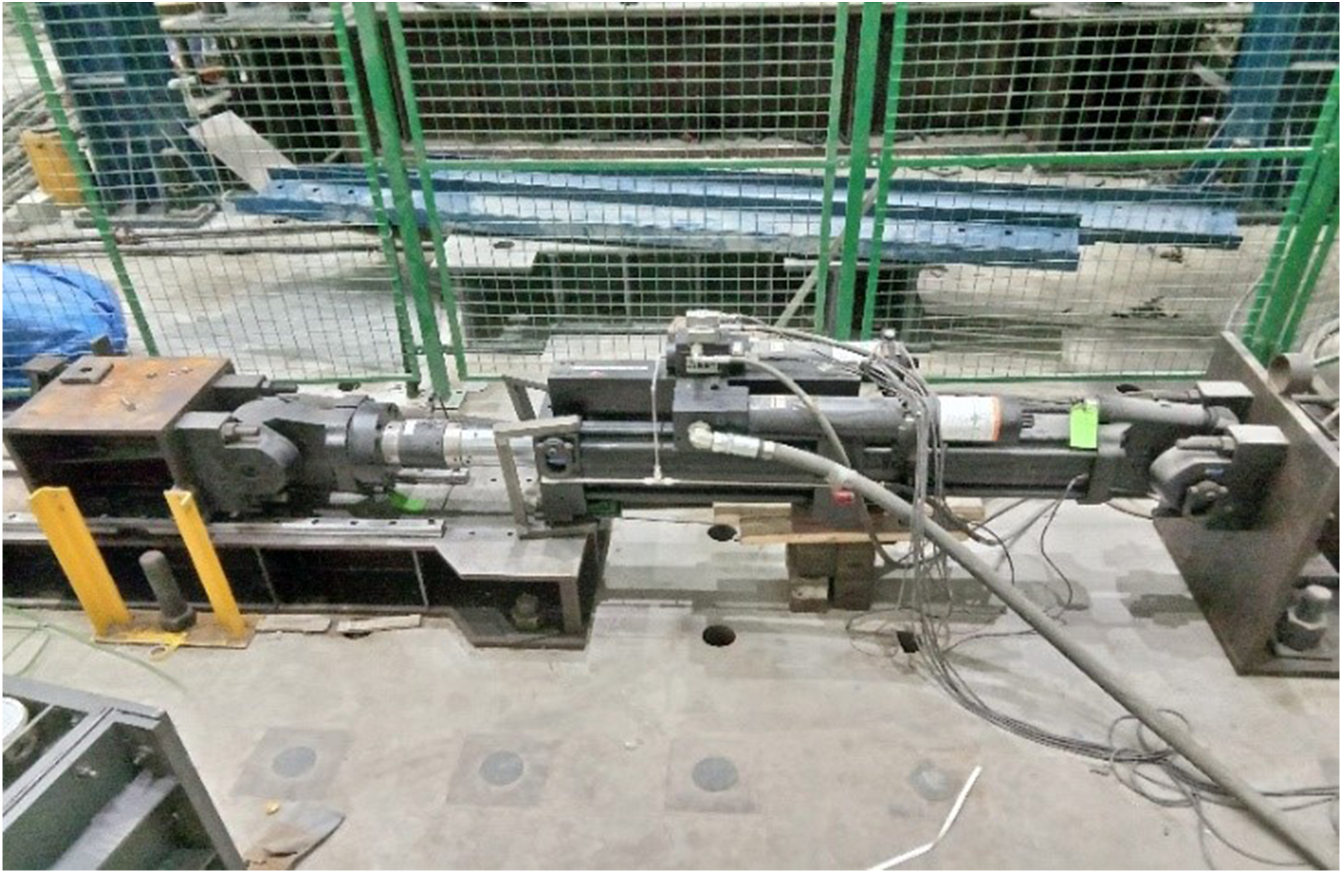

3.2. Identification of servo-hydraulic system model

In this section, the transfer function of the real plant (servo-hydraulic system) is identified to obtain the FF compensator. The frequency response of the servo-hydraulic plant (Figure 3) can be obtained by exciting the plant with a band-limited white noise (BLWN) of 0–50 Hz. For the frequency response (magnitude and phase) of the real plant, we used the “tfestimate” function in MATLAB to calculate it. For the identification of the system transfer function $(G_{ID} (s))$ , we used the “system identification toolbox” in MATLAB to get the transfer function by importing the input (BLWN of 0–50 Hz) and output (measured displacement) of the real plant in time domain.

Figure 3.

Frequency response of real plant and identified transfer function.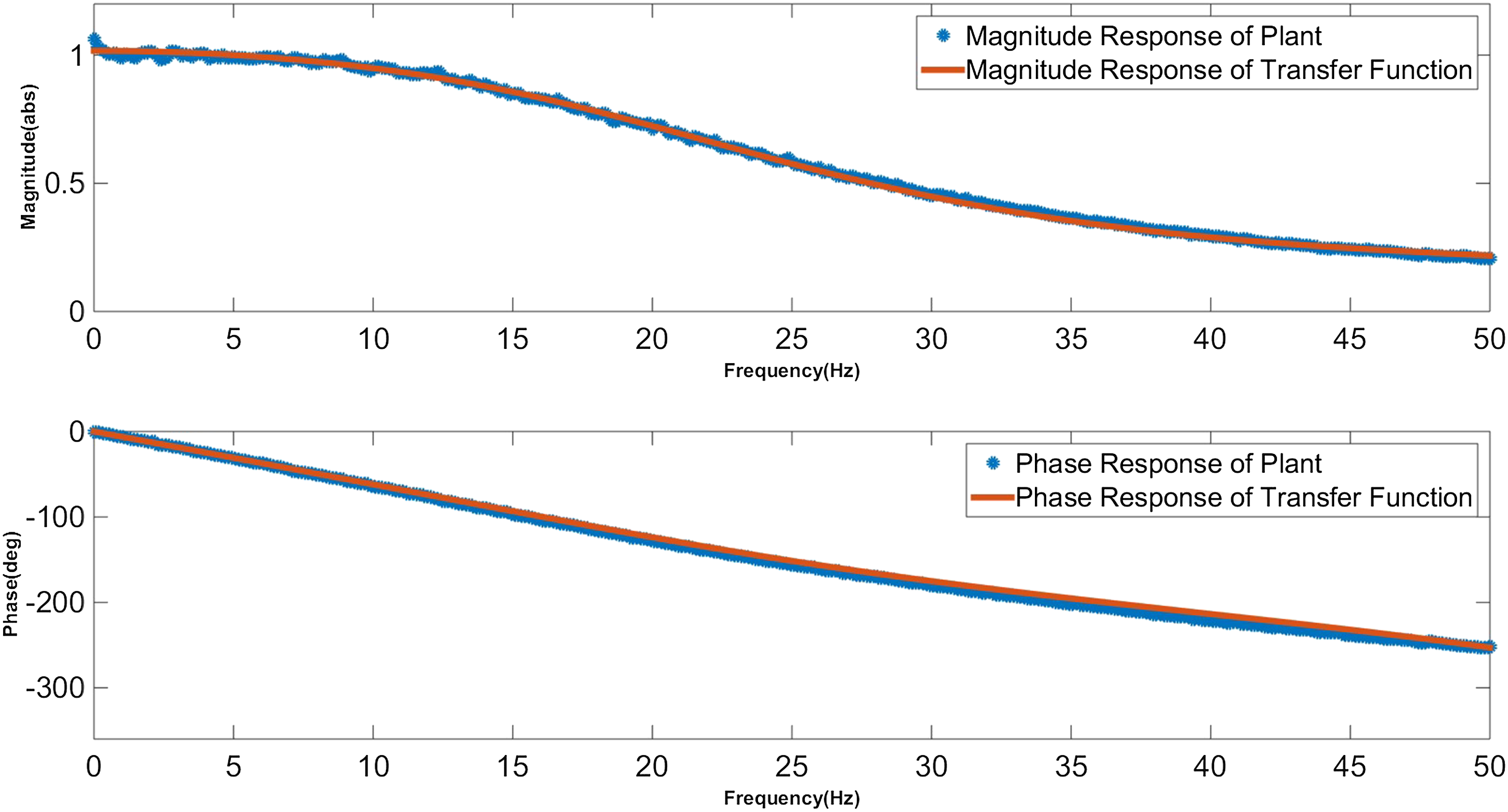

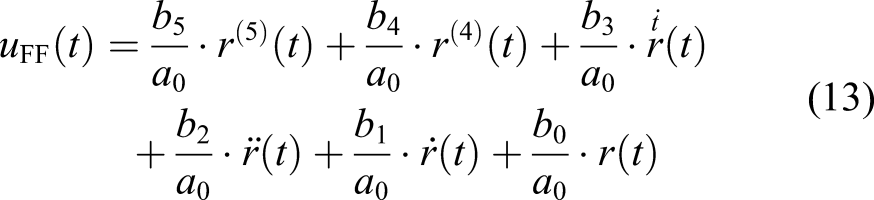
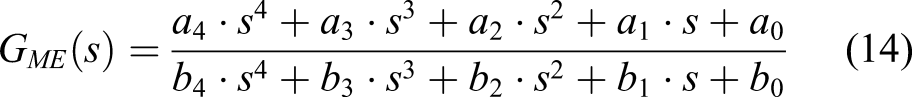
The identified transfer function, $(G_{ID} (s))$ , is

G_{I D} (s) = \frac{a_{0}}{b_{5} s^{5} + b_{4} s^{4} + b_{3} s^{3} + b_{2} s^{2} + b_{1} s + b_{0}}

(11)

where

a_{0} = 4.733 \times 10^{11}

b_{5} = 1

b_{4} = 499

b_{3} = 2.46 \times 10^{5}

b_{2} = 6.04 \times 10^{7}

b_{1} = 7.96 \times 10^{9}

, and

b_{0} = 4.65 \times 10^{11}

. After getting the

G_{I D} (s)

, we calculated the frequency response of the identified transfer function through the “Bode” function in MATLAB as shown in Figure 3. The transfer function of FF compensation,

G_{FF} (s)

, can be obtained by inverting the identified transfer function

G_{I D} (s)

G_{FF} (s) = \frac{b_{5}}{a_{0}} \cdot s^{5} + \frac{b_{4}}{a_{0}} \cdot s^{4} + \frac{b_{3}}{a_{0}} \cdot s^{3} + \frac{b_{2}}{a_{0}} \cdot s^{2} + \frac{b_{1}}{a_{0}} \cdot s + \frac{b_{0}}{a_{0}}

(12)

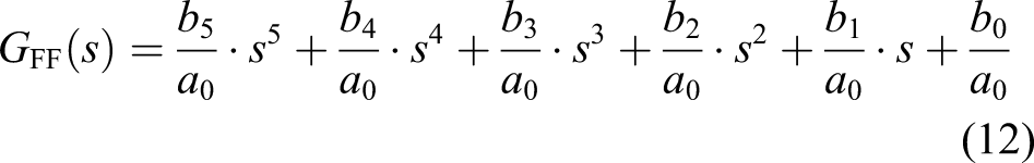
Rewriting equation (12) into the time domain yields

u_{FF} (t) = \frac{b_{5}}{a_{0}} \cdot r^{(5)} (t) + \frac{b_{4}}{a_{0}} \cdot r^{(4)} (t) + \frac{b_{3}}{a_{0}} \cdot \overset{⃛}{r} (t) + \frac{b_{2}}{a_{0}} \cdot \ddot{r} (t) + \frac{b_{1}}{a_{0}} \cdot \dot{r} (t) + \frac{b_{0}}{a_{0}} \cdot r (t)

(13)

3.3. Identification of $G_{ME} (s)$ model

In this section, the identification process and method of $G_{M E} (s)$ is introduced. As seen from equation (6), the input of $G_{M E} (s)$ is the command signal compensated by the FF compensator, and the output is the tracking error between the measured displacement and the command signal. After adding the obtained FF compensator to the control loop, we can get the input and output of $G_{M E} (s)$ . Consequently, the frequency response of the transfer function, $G_{M E} (s)$ , can be obtained by “tfestimate” function in MATLAB as shown in Figure 4.

Figure 4.

Frequency response of transfer function 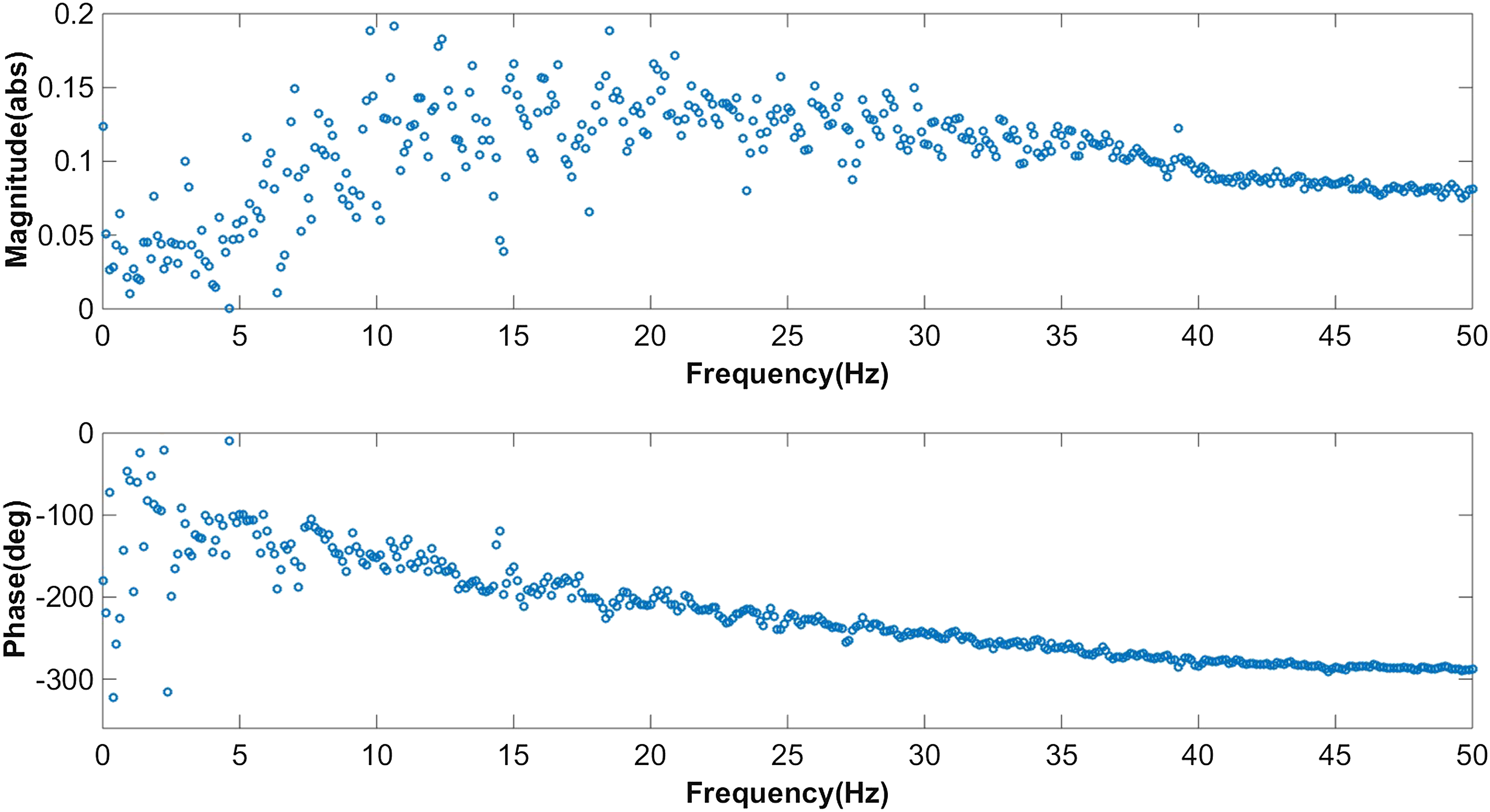$G_{ME} (s)$ .

It can be seen that the frequency response of $G_{M E} (s)$ shows dispersion at low frequencies (below 15 Hz, in this case). However, the trend of $G_{M E} (s)$ remains identifiable. After comparing the results of several methods, we proposed the following method to obtain the transfer function $G_{M E} (s)$ .

Step 1

Take the lower envelope (lower bound) points of magnitude and the upper envelope (upper bound) points of phase, which are shown in Figure 5. The envelope points are obtained by calculating the extreme points of the data points once and then calculating the extreme points again of the first-order extreme points obtained. These second-order extreme points are the envelope points.

Figure 5.

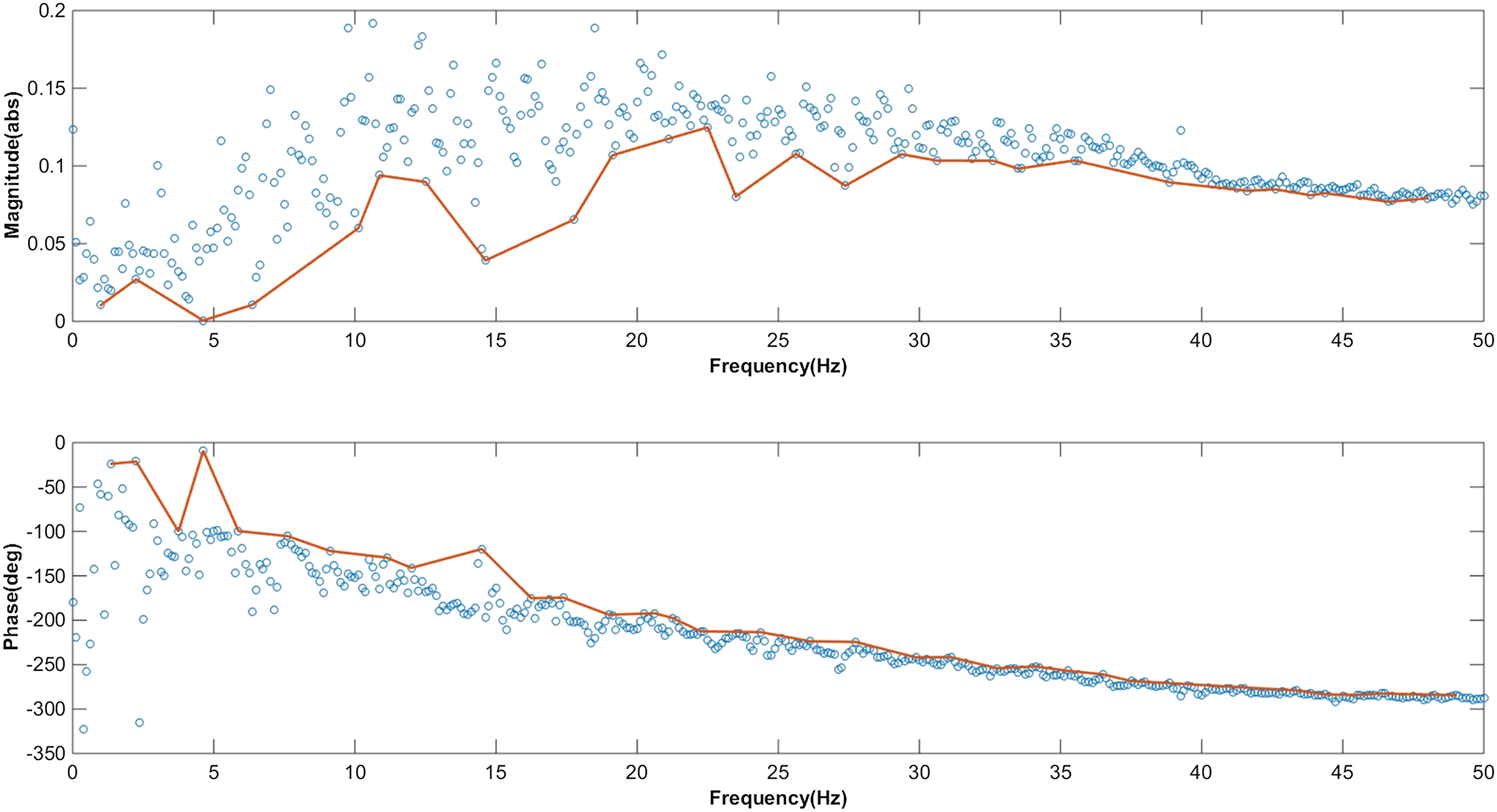
Lower envelope points of magnitude and upper envelope points of phase.

Step 2

Fit the envelope points obtained by the curve fitting toolbox in MATLAB to get the fitting curve, which is shown in Figure 6. This fitting curve is regarded as the frequency response of $G_{M E} (s)$ .

Figure 6.

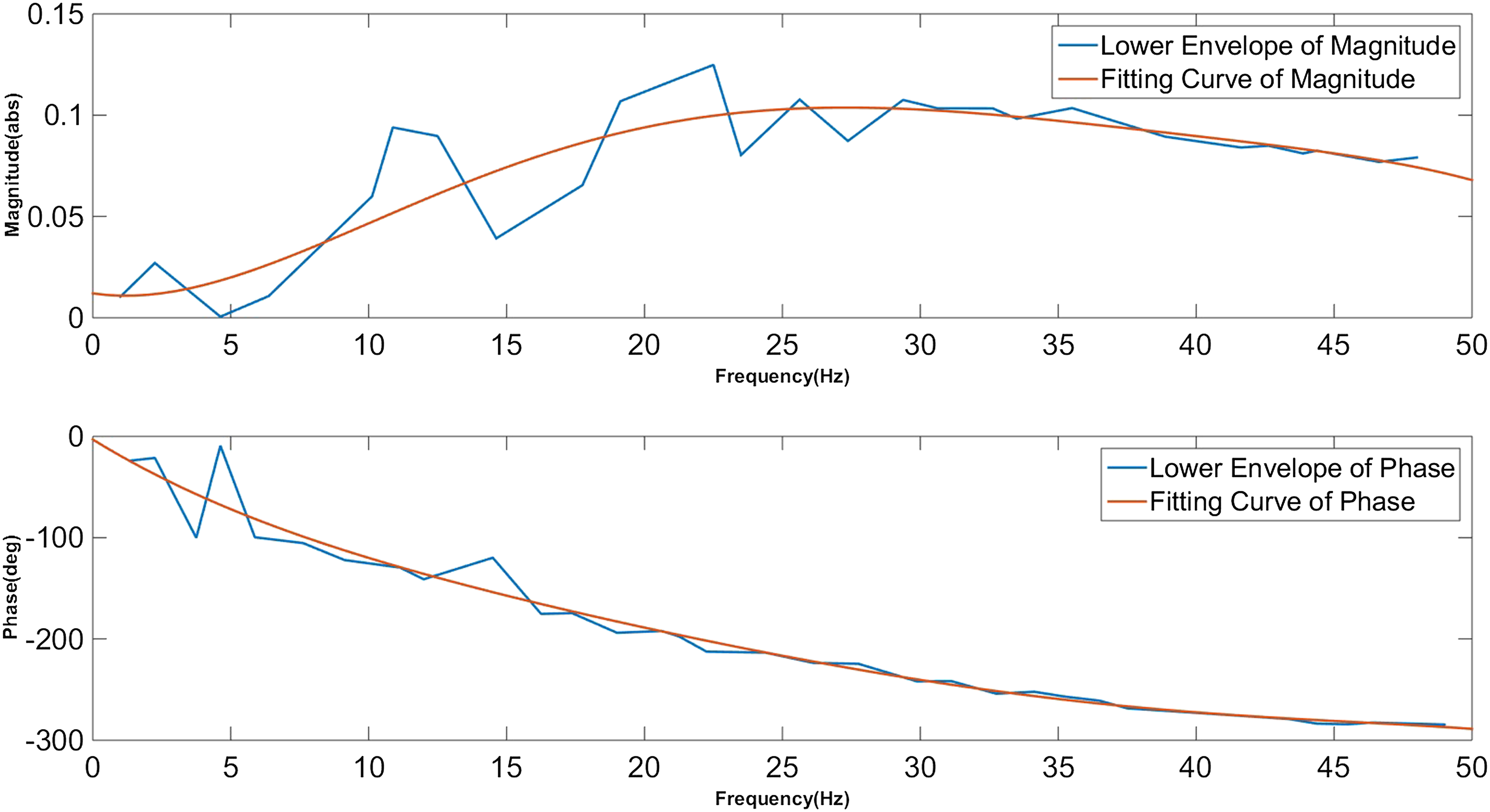
Fitting the frequency response of $G_{ME} (s)$ .

Step 3

After obtaining the frequency response of $G_{M E} (s)$ , we used the “frd” function in MATLAB to convert the frequency response to the format which was required by the system identification toolbox to identify the transfer functions. The result of identification of $G_{M E} (s)$ is shown in the following formula

G_{M E} (s) = \frac{a_{4} \cdot s^{4} + a_{3} \cdot s^{3} + a_{2} \cdot s^{2} + a_{1} \cdot s + a_{0}}{b_{4} \cdot s^{4} + b_{3} \cdot s^{3} + b_{2} \cdot s^{2} + b_{1} \cdot s + b_{0}}

(14)

where

a_{4} = 0.0486

a_{3} = - 9.624

a_{2} = 434.3

a_{1} = - 5.95 \times 10^{5}

a_{0} = 2.841 \times 10^{6}

b_{4} = 1

b_{3} = 271.4

b_{2} = 7.562 \times 10^{4}

b_{1} = 8.906 \times 10^{6}

, and

b_{0} = 7.412 \times 10^{8}

. Hence, the two-stage compensation method is obtained by combining

G_{M E} (s)

and

G_{FF} (s)

according to Figure 1.

4. Validation results and discussion

To verify the effect of the two-stage method proposed in this article, we compared it with the FF compensator in the model-based FF–FB method. The reasons for not considering the feedback in the model-based FF–FB actuator control are as follows.

The two-stage method proposed in this article was developed based on the FF compensator in the model-based FF–FB method. It is more convincing to compare it with the FF compensator, directly.

Fermandois Cornejo et al. (2018) mentioned that the linear quadratic Gaussian (LQG) regulator does not offer any reference tracking guarantee, and the FF compensator is the only instrument responsible for the reference tracking in the context of RTHS testing.

The FF compensator proposed in this article can be additionally combined with the feedback loop such as that in the LQG method and reduce the tracking error. This concept is shown in Section 5.

4.1. Tracking performance in time domain

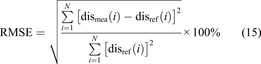
To prove the compensation effect of the two-stage algorithm proposed in this study, we first analyzed its effect in the time domain. A root mean square error (RMSE) was used to quantitatively analyze the effect of compensation delay. In addition, the synchronization plot was used to qualitatively evaluate the effects of the two methods. A total of eight conditions were tested, including BLWNs and chirp. In the following results, test cases denoted by “W” and “C” represent BLWN and chirp, respectively. The following numbers indicate the frequency bandwidth of the excitation. For example, W10 indicates that the excitation is 0–10 Hz BLWN.

The expression of the RMSE indicator is as follows

RMSE = \sqrt{\frac{\sum_{i = 1}^{N} {[{dis}_{mea} (i) - {dis}_{ref} (i)]}^{2}}{\sum_{i = 1}^{N} {[{dis}_{ref} (i)]}^{2}}} \times 100 %

(15)

It can be seen from Table 1 that for the BLWNs below 10 Hz, there is almost no difference between the two methods. The values of the RMSE are all less than 5%, which means that (Figure 7) the tracking performance is in a relatively ideal state. However, when the input frequency increases from 10 Hz to 30 Hz, the RMSE value of the FF method increases from 3.2% to 17.6%. The RMSE value of the two-stage method increases from 2.24% to 8.15%. Moreover, the RMSE of the FF method is more than twice that of the two-stage method in W30.

Table 1.

Root mean square error value of feedforward method and two-stage method (%).

	W1	W5	W10	W15	W20	W25	W30	C20
Feedforward	1.38	1.45	3.20	6.36	9.06	12.86	17.60	12.73
Two-stage	2.27	2.13	2.24	3.99	4.38	5.50	8.55	6.04

Figure 7.

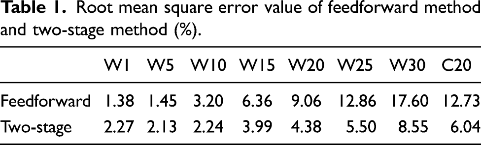
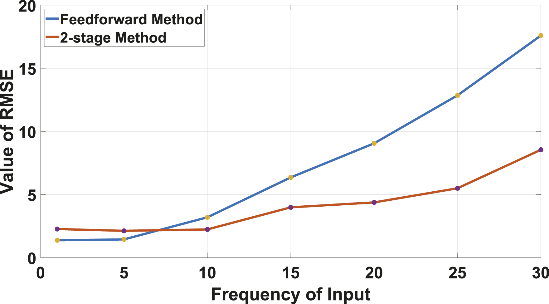
Root mean square error values of feedforward and two-stage compensate methods.

The second evaluation indicator is the synchronization plot, which is a qualitative indicator. The synchronization plot for each case is shown in Figure 8. When the BLWN is lower than 10 Hz, the plot is essentially a straight line at an angle of 45°. In other words, there is not much difference in terms of effectiveness between the two methods for BLWNs lower than 10 Hz. For BLWNs above 10 Hz, the coverage areas drawn by the two-stage method are smaller than those drawn by the FF method. These results imply that the effectiveness of the two-stage method is better than that of the FF method when the excitations are above 10 Hz.

Figure 8.

Synchronization plots of experiment cases.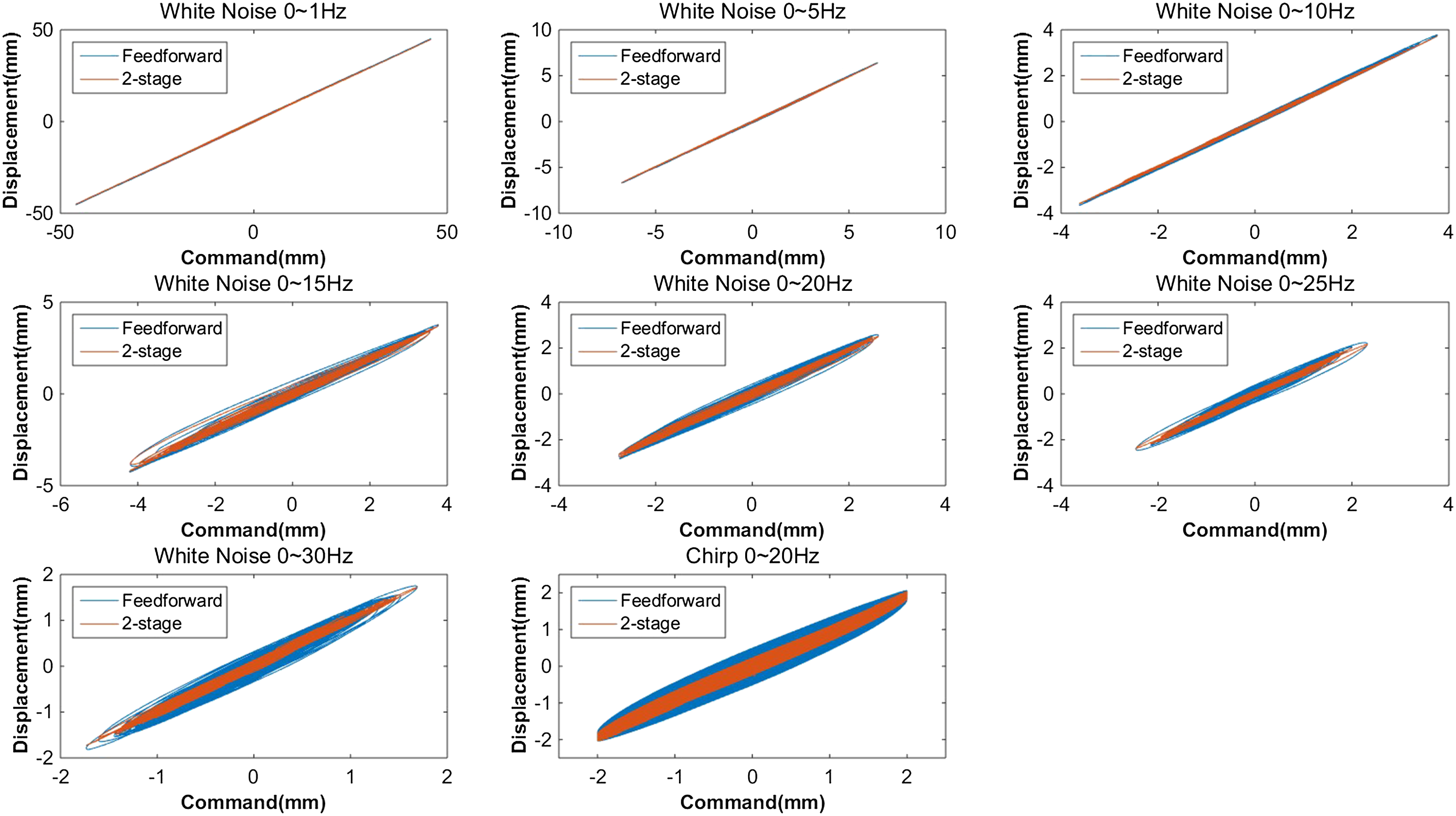

4.2. Tracking performance in frequency domain

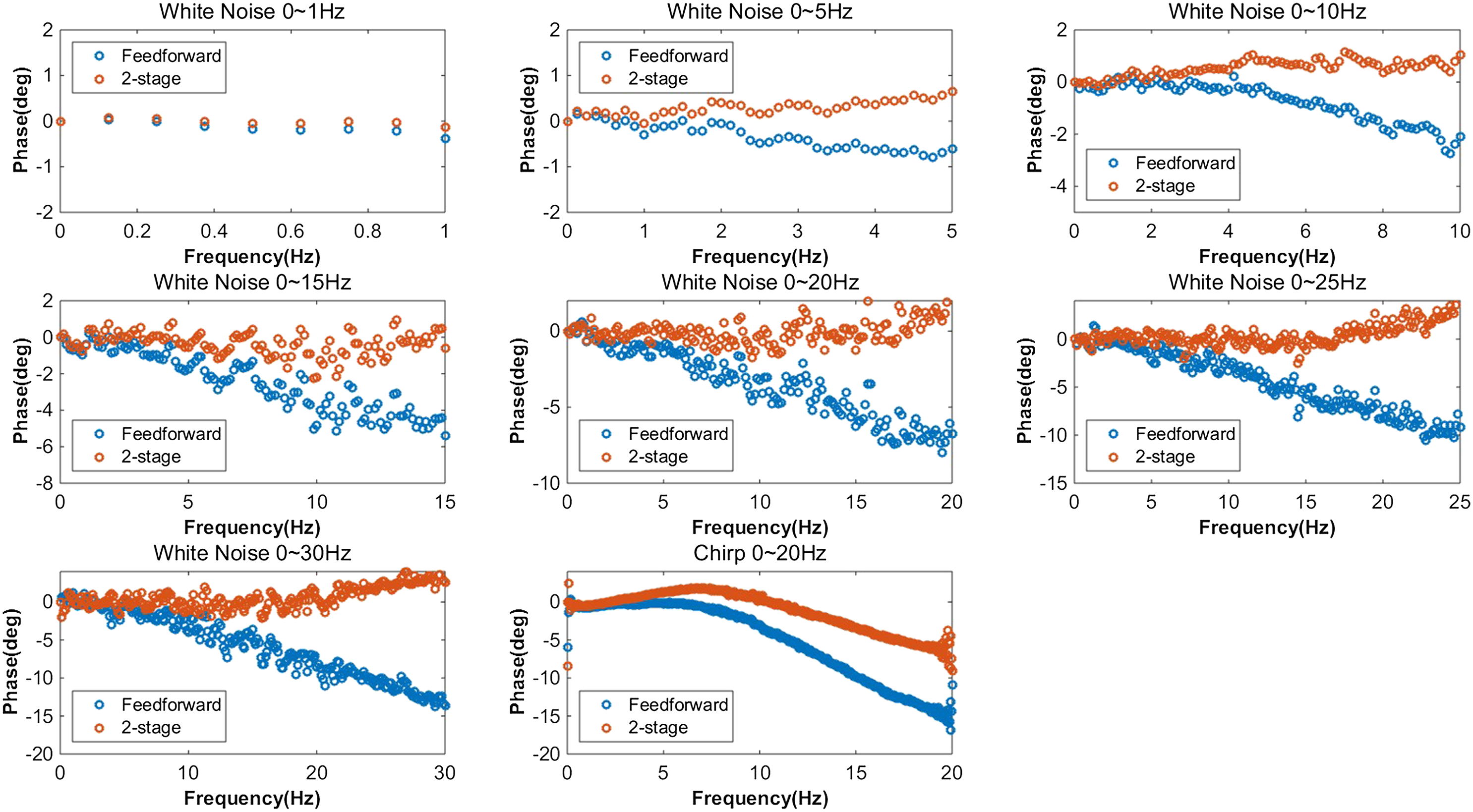
In this section, we evaluate the effects of the two methods from the perspective of frequency domain. The magnitude and phase are shown in Figures 9 and 10, respectively.

Figure 9.

Magnitude comparison of feedforward and two-stage compensate methods.

Figure 10.

Phase comparison of feedforward and two-stage compensate methods.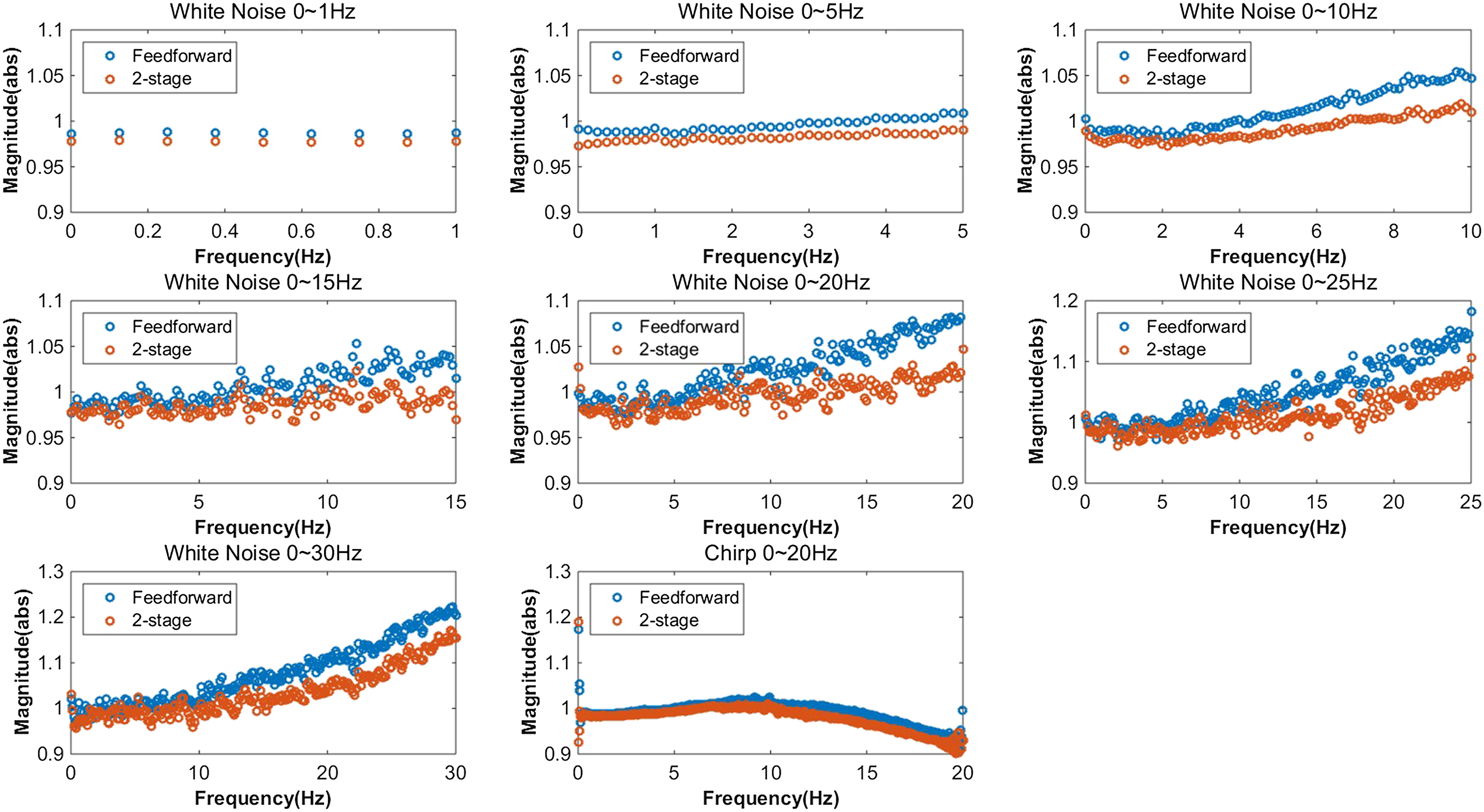

In Figure 9, when the BLWNs are below 10 Hz, the magnitudes of the two methods are approximately one. For BLWNs above 10 Hz, the effect of the two-stage method is better than that of the FF method in terms of magnitude. For instance, for a BLWN of 0–30 Hz, the maximum magnitude response of the FF method is 1.22, whereas that of the two-stage method is 1.15.

In Figure 10, for each case, the phase lag compensated by the two-stage method is distinctly lower than that compensated by the FF method, especially in the high-frequency bandwidth. The phase responses compensated by the two-stage method in every condition are within $\pm$ 5°. However, the phase response remains greatly attenuated after compensation by the FF method. For instance, for a BLWN of 0–30 Hz, the maximum phase lag compensated by the FF method is 15°.

5. RTHS of two-story frame

5.1. Division of substructures

After verifying the advantages of the two-stage method proposed in this study, we applied the method to an RTHS of a double-layer frame to confirm its compensation effect on time delay. In the RTHS, the second layer of the frame was selected as the PS, and the bottom layer was the NS, as shown in Figure 11.

Figure 11.

Division of substructures in real-time hybrid simulation.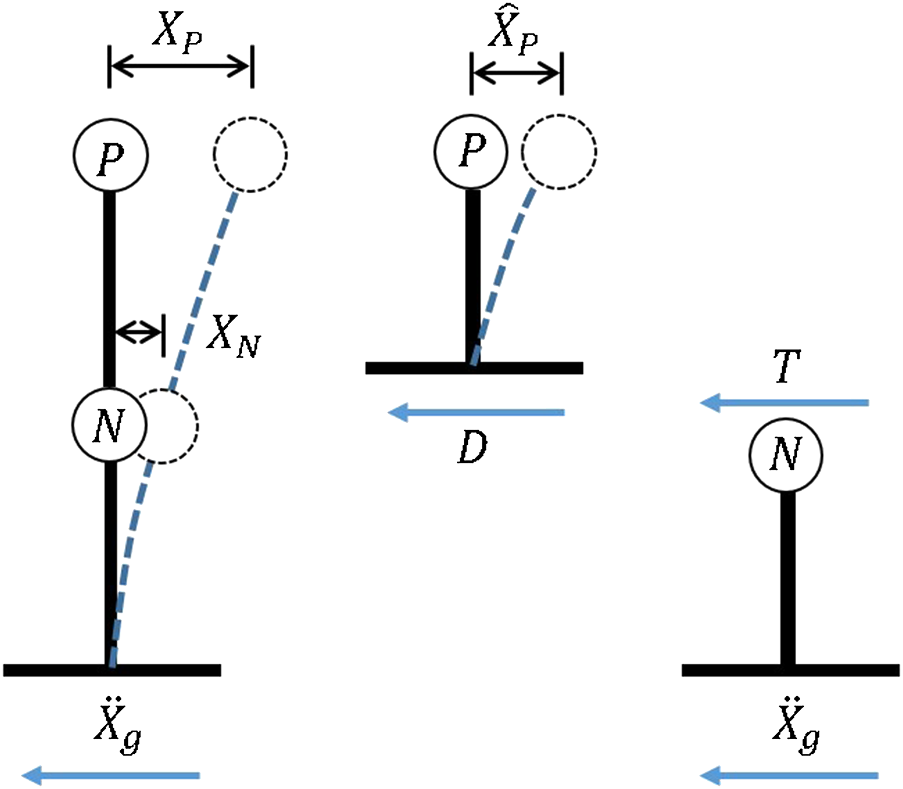

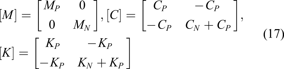
The equation of motion (EOM) of the overall structure is shown in equation (16)

[M] {\ddot{X}} + [C] {\dot{X}} + [K] {X} = {P}

(16)

[M] = [\begin{matrix} M_{P} & 0 \\ 0 & M_{N} \end{matrix}], [C] = [\begin{matrix} C_{P} & - C_{P} \\ - C_{P} & C_{N} + C_{P} \end{matrix}], [K] = [\begin{matrix} K_{P} & - K_{P} \\ - K_{P} & K_{N} + K_{P} \end{matrix}]

(17)

{P} = {- M_{P} {\ddot{X}}_{g}, - M_{N} {\ddot{X}}_{g}}^{T}

(18)

where [M] is the mass matrix, [C] is the damping matrix, [K] is the stiffness matrix, and {P} is the external force matrix.

{\ddot{X}} = {{\ddot{X}}_{P}, {\ddot{X}}_{N}}^{T}

{\dot{X}} = {{\dot{X}}_{P}, {\dot{X}}_{N}}^{T}

, and

{X} = {X_{P}, X_{N}}^{T}

The EOM of the entire structure is divided into the NS equation (19) and PS equation (22)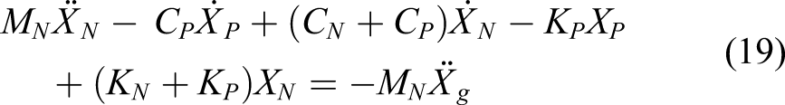

M_{N} {\ddot{X}}_{N} - C_{P} {\dot{X}}_{P} + (C_{N} + C_{P}) {\dot{X}}_{N} - K_{P} X_{P} + (K_{N} + K_{P}) X_{N} = - M_{N} {\ddot{X}}_{g}

(19)

Equation (19) is transformed to obtain equations (20) and (21)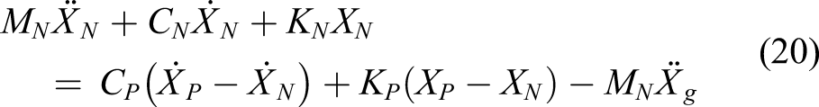

M_{N} {\ddot{X}}_{N} + C_{N} {\dot{X}}_{N} + K_{N} X_{N} = C_{P} ({\dot{X}}_{P} - {\dot{X}}_{N}) + K_{P} (X_{P} - X_{N}) - M_{N} {\ddot{X}}_{g}

(20)

M_{N} {\ddot{X}}_{N} + C_{N} {\dot{X}}_{N} + K_{N} X_{N} = C_{P} \hat{\dot{X}} + K_{P} \hat{X} - M_{N} {\ddot{X}}_{g}

(21)

where

\hat{X}

is the displacement of the PS relative to the NS and

C_{P} \hat{\dot{X}} + K_{P} \hat{X} = T

is the external force of the NS.

The PS equation is as follows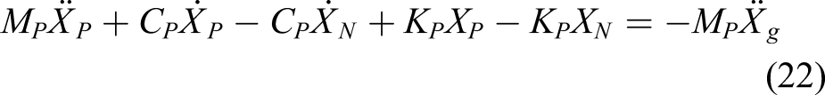

M_{P} {\ddot{X}}_{P} + C_{P} {\dot{X}}_{P} - C_{P} {\dot{X}}_{N} + K_{P} X_{P} - K_{P} X_{N} = - M_{P} {\ddot{X}}_{g}

(22)

Equation (22) is transformed to obtain equations (23) and (24).

M_{P} {\ddot{X}}_{P} - M_{P} {\ddot{X}}_{N} + C_{P} {\dot{X}}_{P} - C_{P} {\dot{X}}_{N} + K_{P} X_{P} - K_{P} X_{N} = - M_{P} {\ddot{X}}_{g} - M_{P} {\ddot{X}}_{N}

(23)

M_{P} \hat{\ddot{X}} + C_{P} \hat{\dot{X}} + K_{P} \hat{X} = - M_{P} ({\ddot{X}}_{g} + {\ddot{X}}_{N})

(24)

From the above analysis, the displacement at the bottom of the PS is the absolute displacement at the top of the NS, that is, $D = X_{g} + X_{N}$ . The external force on the top of the NS is $T = C_{P} \hat{\dot{X}} + K_{P} \hat{X}$ . At the same time, the bottom of the NS is subjected to the earthquake ground motion.

5.2. Test setup

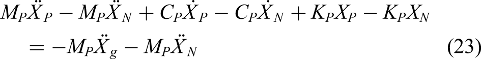
In this RTHS, the PS was a steel frame, as shown in Figure 12. After the identification of the structure, the stiffness of the PS was obtained as $K_{P} = 217.4$ N/m. The mass was $M_{P} = 5 kg$ and the damping was $C_{P} = 1.32 Ns / m$ . The mass of the PS was obtained by weighting. The stiffness can be obtained by applying a horizontal load on the top mass of the PS and stiffness equals load/displacement. The damping can be calculated by the following equation: $C = 2 M ζ \sqrt{K / M}$ , where $ζ$ is the damping ratio which was obtained by the free decay oscillation method, and in this article, the damping ratio is 0.02. Considering the stability of RTHS (Maghareh et al., 2013, 2014) and the safety of the experiment, we took the parameters of the NS as follows: the stiffness of the NS was taken as $K_{N} = 2174 N / m$ , mass was $M_{N} = 50 kg$ , and damping was $C_{N} = 65.94 Ns / m$ . The El Centro earthquake record was selected as the excitation and the magnitude of this seismic acceleration and was reduced by a factor of 10.

Figure 12.

Physical substructure.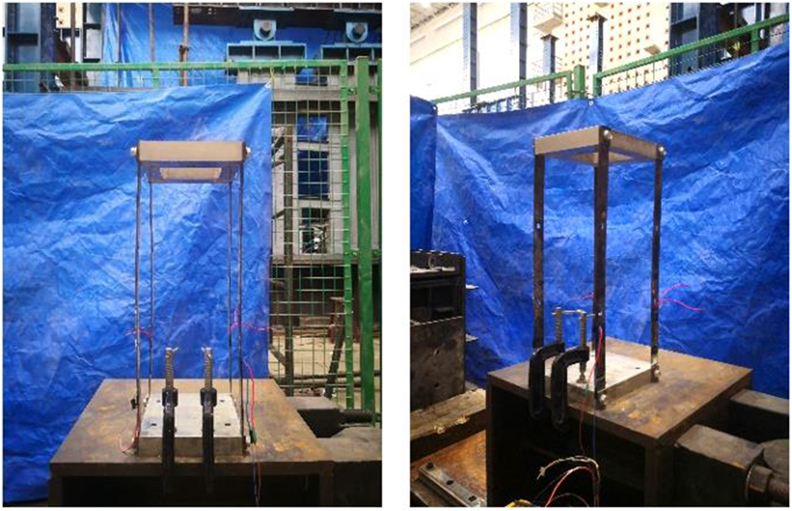

In this RTHS, the CR integral algorithm (Chen and Ricles, 2008) was used to solve the NS. The strain at the bottom of the structure was measured by strain gauges, and the measured data were sent to the national instruments (NIs) real-time data acquisition (DAQ) system. The data between the controller of hydraulic servo system, SpeedGoat, and NI DAQ system were exchanged through the shared memory boards (SCRAMNet) and optical fibers.

The reaction force $T$ applied to the NS was calculated via the correspondence between strain and shear force. The two-stage method was adopted as the FF controller, and the linear quadratic integral control (LQI) method was adopted as the FB controller. In the model-based FF–FB method, the LQG method was used to bring the deviation states to zero and thus reduce the tracking error. However, compared with LQG, the LQI method directly ensures that the output $y$ tracks the reference command $r$ . Therefore, we can reduce the tracking error by setting the reference $r$ and output of the deviation system $y$ to zero and minus the tracking error, respectively. The block diagram of the LQI method is shown in Figure 13, and the LQI method is detailed in the LQI help file of MATLAB.

Figure 13.

Block diagram of linear quadratic integral control method.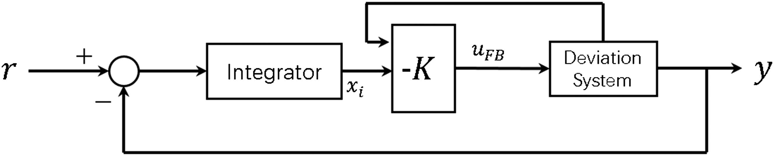

5.3. Analysis of test results

To verify the compensation performance of the two-stage method proposed in this study, the displacement command calculated by the NS and the measured displacement of the actuator were compared and analyzed.

The left figure in Figure 14 reveals the good overlap achieved between the calculated command and measured displacement. Moreover, it can be seen more clearly in the right figure that the synchronization plot is a 45° oblique line and that the time delay is compensated well. From a quantitative perspective, the RMSE value of the command and measured output was calculated to be 1.87%. The errors between the displacement command and measured output were substantially within ±0.2 mm. In summary, from the above analyses of the test results, it can be proven that the two-stage compensation method is an effective time delay compensation method.

Figure 14.

Compensated comparison for real-time hybrid simulation.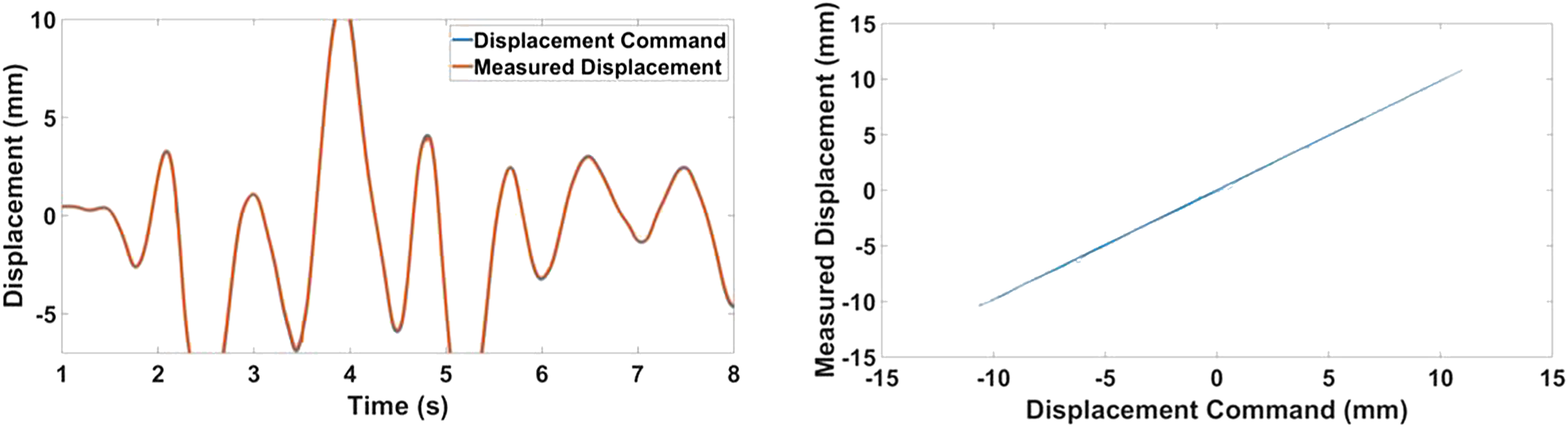

As the size of PS increases, the effect of time delay compensation might be affected. In the case of using relatively small PS, the impact on the loading system is relatively small. Although the original intention of RTHS is to investigate the physical part that cannot be accurately simulated, its response should be very concerned. To truly reproduce the structural response, RTHS requires the loading system to achieve near real-time loading and thus requires that its loading must not be close to or exceed the performance limit of the loading system (usually far below this limit). Please note that as another very important factor, because of the stability consideration of RTHS, it is still not possible to use a large proportion of the PS. And it is far beyond the scope of this article. Therefore, the effect of the PS–NS proportion on the time delay compensation is not addressed here.

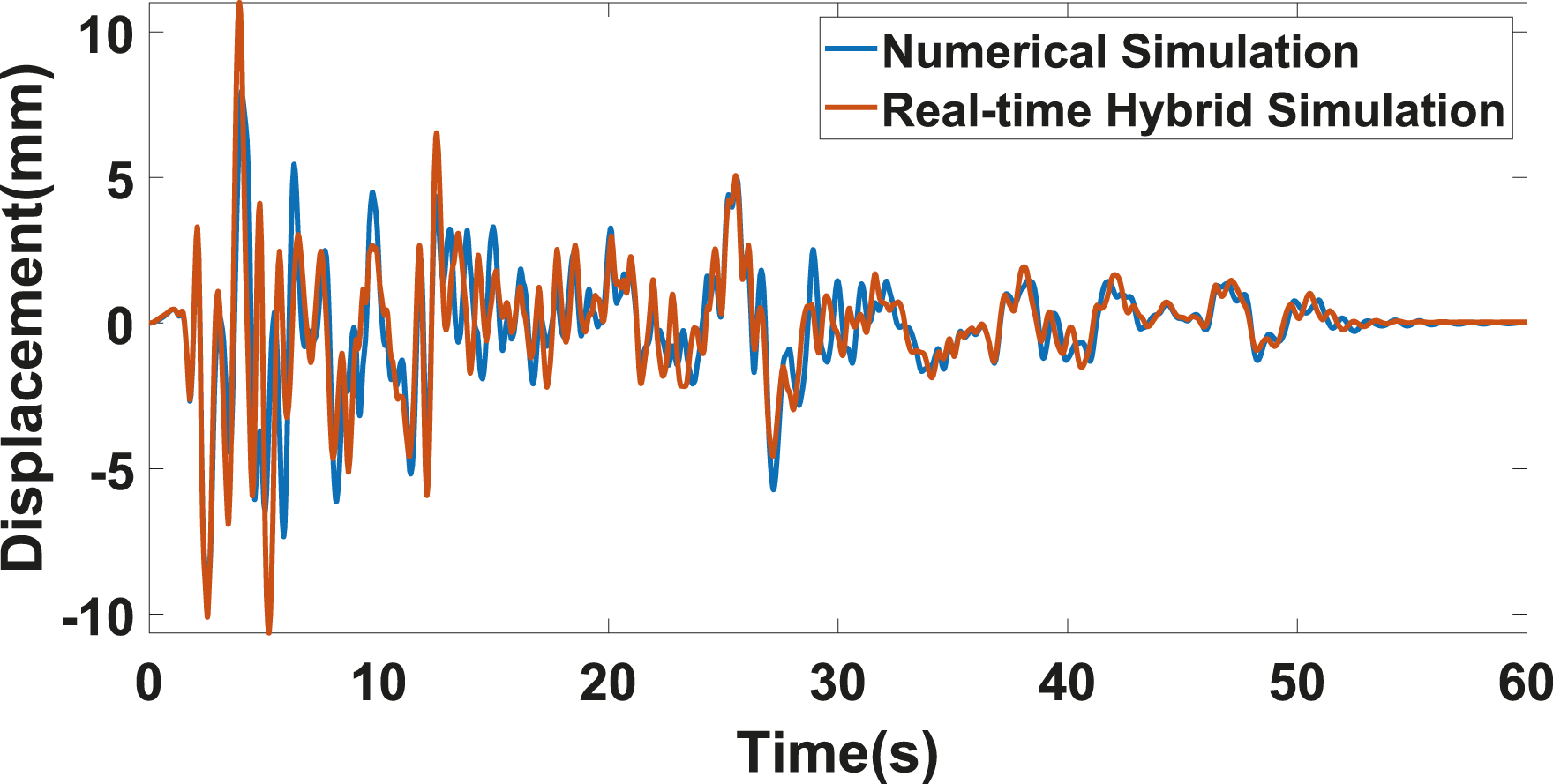
For validation of the proposed method used in RTHS, the absolute displacement responses on top of the NS from the RTHS and the numerical simulation of the entire structure using the EOM were compared in Figure 15. It can be found that the results of the numerical simulation are in good agreement with the results of RTHS. However, there are still some differences between the two results, which are mainly caused by the following aspects.

The PS is a flexible structure with installation errors, and its characteristics cannot be described completely by an EOM with reduced degree of freedoms.

The feedback force signal of the PS using the NI DAQ system contained environmental noises, and with the system uncertainty, they together caused unavoidable disturbances in the control loop.

Figure 15.

Absolute displacement response at the top of numerical substructure.

The results of RTHS and numerical simulation further proved the performance of the time-delay compensation method proposed in this article. By comparing the results, there is a more thorough understanding for the effect of the new compensation method on the accuracy of RTHS technology.

6. Conclusions

Based on the model-based FF–FB control method, we proposed in this study a new two-stage method for RTHS. The two-stage method introduced the error between the model identified and the real plant into the compensator to enhance the compensation performance. Moreover, we performed a comparative analysis of two different methods to confirm the effectiveness of the two-stage method. Furthermore, the efficacy of the proposed method was proved by an RTHS of a frame.

Compared with the model-based FF compensator, the two-stage method can achieve improved time-delay compensation performance, especially in the high-frequency bandwidth. This point was confirmed by comparing the results of the two methods both in the time domain and frequency domain.

The results of the RTHS proved that the two-stage method can effectively control the tracking error to achieve good tracking performance.

The proposed method additionally provided a new idea for the model-based time-delay compensation method. By considering the difference between the identified model and the real plant, the model-based compensation method can be further modified and improved to achieve enhanced compensation performance.

Footnotes

Declaration of conflicting interests

The authors declared no potential conflicts of interest with respect to the research, authorship, and/or publication of this article.

Funding

The authors disclosed receipt of the following financial support for the research, authorship, and/or publication of this article: The authors appreciate anonymous reviewers for critical reading of the manuscript and for offering many useful suggestions that led to significant improvement of the paper. The supports for this research provided by the National Key R & D Program of China (grant nos. 2018YFC1504306 and 2016YFC0701108) and the National Natural Science Foundation of China (grant nos. 51427901 and 51678407) also acknowledged.

ORCID iD

Ning Li

References

Ashasi-Sorkhabi

Malekghasemi

Mercan

(2015) Implementation and verification of real-time hybrid simulation (RTHS) using a shake table for research and education. Journal of Vibration and Control 21(8): 1459–1472.

Carrion

Spencer

Jr (2007) Model-Based Strategies for Real-Time Hybrid Testing. Urbana, IL: Newmark Structural Engineering Laboratory, University of Illinois at Urbana-Champaign.

Chae

Kazemibidokhti

Ricles

(2013) Adaptive time series compensator for delay compensation of servo-hydraulic actuator systems for real-time hybrid simulation. Earthquake Engineering & Structural Dynamics 42(11): 1697–1715.

Chen

(2007) Development and Numerical Simulation of Hybrid Effective Force Testing Method. Bethlehem, PA: Lehigh University.

Chen

Ricles

(2008) Development of direct integration algorithms for structural dynamics using discrete control theory [J]. Journal of Engineering Mechanics 134(8): 676–683.

Chen

Ricles

(2009) Improving the inverse compensation method for real-time hybrid simulation through a dual compensation scheme. Earthquake Engineering & Structural Dynamics 38(10): 1237–1255.

Chen

Ricles

(2010) Tracking error-based servohydraulic actuator adaptive compensation for real-time hybrid simulation. Journal of Surgical Education 136(4): 432–440.

Chen

Ricles

(2012) Large-scale real-time hybrid simulation involving multiple experimental substructures and adaptive actuator delay compensation. Earthquake Engineering & Structural Dynamics 41(3): 549–569.

Chen

Ricles

Marullo

, et al. (2009) Real-time hybrid testing using the unconditionally stable explicit CR integration algorithm. Earthquake Engineering & Structural Dynamics 38(1): 23–44.

10.

Chen

P-C

Chang

C-M

Spencer

, et al. (2015) Adaptive model-based tracking control for real-time hybrid simulation. Bulletin of Earthquake Engineering 13(6): 1633–1653.

11.

Darby

Williams

Blakeborough

(2002) Stability and delay compensation for real-time substructure testing. Journal of Engineering Mechanics 128(12): 1276–1284.

12.

Fermandois Cornejo

Spencer

Jr (2018) Development and Implementation of a Multi-Axial Real-Time Hybrid Simulation Framework. Urbana, IL: University of Illinois at Urbana-Champaign.

13.

Hayati

Song

(2016) Discrete-Time Compensation Technique for Real-Time Hybrid Simulation. Cham: Springer, Vol. 8, 351–358.

14.

Horiuchi

Inoue

Konno

, et al. (1999) Real-time hybrid experimental system with actuator delay compensation and its application to a piping system with energy absorber. Earthquake Engineering & Structural Dynamics 28(10): 1121–1141.

15.

Horiuchi

Konno

(2001) A new method for compensating actuator delay in real-time hybrid experiments. Philosophical Transactions of the Royal Society of London. Series A: Mathematical, Physical and Engineering Sciences 359(1786): 1893–1909.

16.

Zhou

, et al. (2019a) A novel two-stage time-delay compensation for real-time hybrid testing: simulation and experimental validation. Journal of Vibration and Shock 39: 31–38.

17.

Zhou

(2019b) Time-delay tracing based adaptive compensation algorithm for real-time hybrid testing. Engineering Mechanics 36(7): 38–46.

18.

Liu

Dyke

Liu

H-J

, et al. (2013) A novel integrated compensation method for actuator dynamics in real-time hybrid structural testing. Structural Control and Health Monitoring 20(7): 1057–1080.

19.

Maghareh

Dyke

Prakash

, et al. (2013) Establishing Predictive Indicators for Stability and Performance of SDOF Real-Time Hybrid Simulations [R], Report no IISL-004. West Lafayette, IN: Purdue University.

20.

Maghareh

Dyke

Prakash

, et al. (2014) Establishing a stability switch criterion for effective implementation of real-time hybrid simulation. Smart Structures and Systems 14(6): 1221–1245.

21.

Malekghasemi

Ashasi-Sorkhabi

Ghaemmaghami

, et al. (2015) Experimental and numerical investigations of the dynamic interaction of tuned liquid damper-structure systems. Journal of Vibration and Control 21(14): 2707–2720.

22.

Mirza Hessabi

Ashasi-Sorkhabi

Mercan

(2016) A new tracking error-based adaptive controller for servo-hydraulic actuator control. Journal of Vibration and Control 22(12): 2824–2840.

23.

Nakashima

Masaoka

(1999) Real-time on-line test for MDOF systems. Earthquake Engineering & Structural Dynamics 28(4): 393–420.

24.

Phillips

Spencer

Jr (2012a) Model-based Framework for Real-Time Dynamic Structural Performance Evaluation. Urbana, IL: Newmark Structural Engineering Laboratory, University of Illinois at Urbana-Champaign.

25.

Phillips

Spencer

Jr (2012b) Model-based feedforward-feedback actuator control for real-time hybrid simulation. Journal of Structural Engineering 139(7): 1205–1214.

26.

Phillips

Wierschem

Spencer

Jr (2014) Model-based multi-metric control of uniaxial shake tables. Earthquake Engineering & Structural Dynamics 43(5): 681–699.

27.

Schellenberg

Becker

Mahin

(2013) Hybrid shake table for the testing of midlevel seismic isolation systems. In: Proceedings of the 13th world conference on seismic isolation, energy dissipation and active vibration control of structures, 24–27 September 2013, Sendai, Japan.

28.

Shao

Reinhorn

Sivaselvan

(2010) Real-time hybrid simulation using shake tables and dynamic actuators. Journal of Structural Engineering 137(7): 748–760.

29.

Stehman

Nakata

(2016) IIR compensation in real-time hybrid simulation using shake tables with complex control-structure-interaction. Journal of Earthquake Engineering 20(4): 633–653.

30.

Strano

Terzo

(2016) Actuator dynamics compensation for real-time hybrid simulation: an adaptive approach by means of a nonlinear estimator. Nonlinear Dynamics 85(4): 2353–2368.

31.

Wallace

Wagg

Neild

(2005) An adaptive polynomial based forward prediction algorithm for multi-actuator real-time dynamic substructuring. Proceedings of the Royal Society A: Mathematical, Physical and Engineering Sciences 461(2064): 3807–3826.

32.

Wang

J-T

Gui

Zhu

, et al. (2016) Real-time hybrid simulation of multi-story structures installed with tuned liquid damper. Structural Control and Health Monitoring 23(7): 1015–1031.

33.

Zhang

Phillips

Taniguchi

, et al. (2017) Shake table real-time hybrid simulation techniques for the performance evaluation of buildings with inter-story isolation. Structural Control and Health Monitoring 24(10) e1971.

34.

Zhao

French

Shield

, et al. (2003) Considerations for the development of real-time dynamic testing using servo-hydraulic actuation. Earthquake Engineering & Structural Dynamics 32(11): 1773–1794.

35.

Zhou

Wagg

(2017) Equivalent force control combined with adaptive polynomial‐based forward prediction for real‐time hybrid simulation. Structural Control and Health Monitoring 24(11): e2018.

Improving model-based compensation method for real-time hybrid simulation considering error of identified model

Abstract

Keywords

Highlights

1. Introduction

2. Two-stage FF method

3. Identification procedure of G ME ( s )

3.1. Experimental setup

3.2. Identification of servo-hydraulic system model

3.3. Identification of G ME ( s ) model

4. Validation results and discussion

4.1. Tracking performance in time domain

4.2. Tracking performance in frequency domain

5. RTHS of two-story frame

5.1. Division of substructures

5.2. Test setup

5.3. Analysis of test results

6. Conclusions

Footnotes

Declaration of conflicting interests

Funding

ORCID iD

References

3. Identification procedure of $G_{ME} (s)$

3.3. Identification of $G_{ME} (s)$ model