Rail/wheel rolling noise generation due to parametric excitation

Abstract

When a wheel rolls over a railway rail, it ‘sees’ a varying stiffness downwards because the rail is periodically supported by sleepers, leading to parametric excitation of the rail/wheel system. This study investigates the importance of parametric excitation on railway noise generation. Because the problem is non-stationary, it is modelled in the time domain. Rail and wheel impulse response functions, together with an iteration scheme to match boundary conditions in the rail/wheel contact patch, yield rail and wheel response plus contact force at each wheel position on the rail. Forward velocity and rotation of the elastic wheel are accounted for. Feedback coupling between response and force takes part in the excitation. Numerical simulations show that, for a rail on stiff pads, parametric excitation is a major excitation mechanism, above all leading to increased excitation and noise levels in a broad frequency region around the pinned–pinned frequency.

Keywords

Railway noise rolling noise parametric excitation periodically supported rail pinned–pinned frequency time domain rail vibration

1. Introduction

Rail/wheel rolling noise is generated during the rolling process due to small-scale roughnesses on the rail/wheel running surfaces. Another excitation mechanism is parametric excitation due to the varying track stiffness because the rail is periodically supported on sleepers. A third mechanism is the feedback coupling mechanism between wheel/rail response and contact force. Of these three effects, roughness-induced excitation has been thoroughly investigated by Remington (1987a, 1987b) and Thompson (2009) and it is also known to be the main cause for rail/wheel rolling noise.

Parametric excitation increases noise generation at low frequencies, at the sleeper-passing frequency, and at higher frequencies around the rail pinned–pinned frequency, which occurs around 1 kHz, (Nordborg, 1998a, 2002) and (Wu and Thompson 2004, 2006). Parametric excitation can be neglected for a softly padded rail, Nordborg and Koh (2016), but it is shown in this study that for a rail on stiff pads, parametric excitation may be a major excitation mechanism.

The model presented in this study is more realistic than those in the references cited above because it also includes the wheel resonances, as opposed to the simpler rigid wheel mass models used before. In addition, the influences of high train speeds on rail and wheel dynamics are included in the moving rail Green’s function, as well as the rotating wheel Green’s function. Thus, the model adopts a Green’s function approach. Those Green’s functions are transformed to the time domain, represented there by impulse response functions. In the time domain, the system state variables (contact force and rail/wheel response) are computed for each time step by an iteration process, after which time and wheel position on the rail are incremented by a small amount. Because the model operates in the time domain, non-stationary processes (parametric excitation, feedback coupling and non-linear effects) can be accounted for. A frequency-domain model is incapable of doing that. The current model has previously been used to investigate non-linear rail/wheel contact mechanics during rolling (Lundberg et al., 2016). Similar Green’s function approaches of the railway track have been used to study the effects of curve squeal and impacts of wheel flats, Pieringer (2014) and Mazilu (2007), and on the effect of introducing rail dampers on the rail/wheel interaction (Sheng et al., 2016). The wheel was always a rigid mass in those investigations.

The simulation calculations of the current model result in broadband contact force and rail/wheel response spectra, as opposed to the discrete response spectra obtained in previous studies on the same topic mentioned above.

Parts of the current model have previously been presented in detail in a number of studies and conference proceedings (see the reference list at the end of the article) and are summarized in the following. An introduction to the theory of parametric excitation can be found in the book by Nayfeh and Mook (1979).

2. Theory

2.1. Rail

The rail is modelled as a uniform Euler beam of infinite length, resting on identical supports (sleepers) at periodic intervals (Figure 1) (Nordborg, 1998b). The Euler beam theory can be used up to at least 2000 Hz if the bending stiffness is reduced by an appropriate amount (Nordborg and Verhelst, 2019). The spacing between (the centres of) two sleepers is l. The supports are modelled as lumped mass-spring-damping systems. The rail is thus restrained to move in the vertical direction. Rotational constraints (Nordborg, 1999) as well as sleeper modes (Dalenbring, 1995) can also be included in the support description. The response, that is the vertical rail deflection, at coordinate x due to a stationary harmonic unit point force δ(x − x₀) at x₀, by definition is the Green’s function, G(x|x₀). As the rail–sleeper system is periodic with period l, according to Floquet’s theorem, Green’s function is a linear combination of solutions having the form defined by

Y (x + n l) = Y (x) e^{n g}

(1)

where the complex coefficient g determines vibration propagation and sound radiation from the rail. Integer n denotes the number of the sleeper bay. Waves (propagating to the right) decay if

ℜ (g) \leq 0

; such frequency ranges are called stopbands. On the other hand, if

ℜ (g) ≃ 0

(some damping is always present), the waves propagate almost unattenuated; these frequency ranges are called passbands.

Figure 1.

Discretely supported rail, with a wheel moving (rolling) forward, exciting rail and wheel into vibrations and noise radiation, due to surface roughnesses and parametric excitation.

Because Green’s function here has unit m/N, it represents the (point or transfer) receptance of the rail. The integral of vertical rail vibrations over the whole length of the rail, the energy spectral density ESD₁ (Nordborg and Koh, 2016) of the rail

{ESD}_{1} = \int_{- \infty}^{\infty} {| G_{ω_{0}} (x | x_{0}) |}^{2} d x

(2)

is an important property determining the amount of radiated noise. Subscript 1 indicates that the rail is excited by a unit point force. This integral, and thus the noise radiation, becomes large when vibrations can propagate unimpeded over long distances in the rail–sleeper system, that is when the real part of the propagation coefficient

ℜ (g) ≃ 0

(see equation (1)). The Track Decay Rate (TDR; Thompson, 2009) determines attenuation of rail vibration per metre rail length, TDR = −20 log(|e^g|)/l (dB/m), which can be rewritten as

TDR = - \frac{20}{ln (10)} \frac{1}{l} ℜ (g)

(3)

Green’s function can be used to calculate rail response Y (vertical vibration) and subsequently also the contact force. Assume the rail is excited by a general force, f(x,t) in the time domain and F(x,ω) in the frequency domain. The solution, vertical rail vibrations at the position x₀, can in the frequency domain be written as

Y (x_{0}, ω) = \int_{- \infty}^{\infty} G_{ω} (x | x_{0}) F (x, ω) d x

(4)

The problem to be solved is to calculate rail and wheel responses, y_r(x₀, t₀) and y_w, as the wheel rolls over the rail, and subsequently the noise radiation during the rolling process. In the time domain, the vertical rail deflection, y_r(x₀, t₀), at the moving point, x₀ = vt₀, (under the wheel) is a convolution of the rail Green’s function in the time domain, the impulse response function g(x, x₀; t, t₀) and the forward moving contact force f(x, t) = f(t) δ (x − vt) (Nordborg, 2002)

y_{r} (x_{0}, t_{0}) = \int \int g (x, x_{0}; t, t_{0}) f (x, t) d x d t

(5)

Green’s function in the time domain, g(x, x₀; t, t₀), is calculated by an inverse Fourier transform of Green’s function in the frequency domain, G(x|x₀).

2.2. Wheel

The wheel response (Nordborg and Kohrs, 2015) is as for the rail, calculated using the (wheel) impulse response function g_w

y_{w} = \int \int g_{w} f d x d t + y_{w, m}

(6)

The excitation force is the same as for the rail because the rail and wheel are in contact. The wheel impulse response function, g_w, is calculated in this study using inverse Fourier transform of point and transfer receptance in the radial direction of the wheel (more details about the calculation algorithm can be found in Klaus (2019)). However, the vertical displacement of the rigid mass of the wheel, y_w,m, is calculated separately by numerically solving the ordinary differential equation (ODE) of the wheel mass acted upon by inertia forces caused by the constant preload force P plus the contact force f (without the preload, caused by the weight of the train on the wheel axle, the wheel would not stay in contact with the rail). Therefore, the rigid mass mode of the modal model describing the frequency response functions (FRFs) of the wheel is excluded from the modal model, and thus not included in the impulse response function, g_w, of the wheel. Separation of the rigid mode and the other higher frequency modes of the wheel is a necessary step to perform the ODE integration mentioned above. In addition, it enables comparison of the effects of these higher wheel modes on the rail/wheel interaction with the response using a simple lumped mass model only (although not done in this study).

2.3. Contact

The compression of the wheel/rail contact region (patch) must simultaneously fulfil two equations. First, it is determined by the vertical rail and wheel deflections and surface roughness, y_s

δ = y_{r} + y_{s} - y_{w}

(7)

Second, according to Hertz, the indentation is a non-linear function of the contact force f, δ_H = δ_H(f). Of course, f ≥ 0 always; f = 0 implies the loss of wheel–rail contact, δ ≤ 0.

The rolling process is simulated by calculation of rail/wheel deflections and contact force at each time step. If δ and δ_H are not equal, the indentation is varied a little, and rail/wheel deflections and contact force are recalculated. Solving

δ - δ_{H} (f) ≃ 0

iteratively yields the contact force f (Nordborg, 2002) for the current time step. When the contact force f finally has been determined, rail and wheel deflections, y_r and y_w, respectively, can also be calculated with the help of the impulse response functions, and the convolutions described in equations (5) and (6). The time and wheel position on the rail is incremented, and the process described above is repeated.

2.4. Surface roughness

To calculate the contact force, we need to know y_s, the vertical deviation of the rail surface from a perfectly smooth rail surface. The roughness of the rail is usually expressed by a roughness amplitude spectrum (dB re. 1 μm) versus roughness wavelength. A random sequence y_s as a function of distance along the rail running surface is generated. The sequence is then processed to ensure that the spectrum takes the same form as the desired roughness amplitude spectrum. It is Fourier transformed to the frequency domain where the spectrum is shaped, then inverse Fourier transformed back to the time domain again. The spectrum used is a combined rail/wheel roughness spectrum, including contact filtering effects (Thompson, 2009).

2.5. Noise radiation

Sound radiation from the rail depends on the total rail vibration. It is shown (Nordborg 1998a) that the energy spectral density (ESD) of vertical rail vibrations excited by a moving force can be estimated by the expression

ESD = \frac{1}{v} S_{F F} {ESD}_{1}

(8)

if v << c_B (the bending wave speed in the rail) and the excitation force F (equation (4)) are periodic along the periodic rail–sleeper system. The factor

1 / v

appeared because the rail is excited by a moving force. The ESD₁ when the rail is excited by a stationary unit point force is defined by equation (2), and S_FF is the power spectral density of the contact force. Force as a function of time was calculated in section Contact above, from which the power spectral density is obtained. The pass-by time T_p, defined by the train length, yields the corresponding power spectral density of vertical rail vibrations

PSD = 1 / v T_{p} S_{F F} {ESD}_{1}

. Sound power W of radiated noise due to vertical rail vibrations also depends on rail width w and radiation efficiency σ

W = ρ_{0} c_{0} σ w ω^{2} \frac{1}{v T_{p}} S_{F F} {ESD}_{1}

(9)

Multiplication by ω² comes from going from vibration displacement to vibration velocity (squared).

3. Numerical simulations

3.1. Application example: time-domain versus frequency-domain models

With numerical simulations, it is shown why a model for prediction of rail/wheel rolling noise at least sometimes has to be performed in the time domain, and not in the frequency domain, to yield valid prediction results. Mostly, railway noise is predicted using frequency-domain models (see e.g. TWINS (Thompson, 2009)) because frequency-domain models have many advantages: they are relatively easy to perform and their calculation times are short. However, the disadvantage is that they sometimes are incapable of describing all relevant effects taking part in the rolling noise generation process, which leads to prediction errors. To illustrate this, numerical simulations with two models, one in the time domain developed in this paper, and the other in the frequency domain, are performed and the results compared and shown below. The frequency-domain model (Nordborg and Koh, 2016) uses the same input FRFs as the time-domain model; however, forward velocity and wheel rotation as well as the interaction between rail/wheel response and contact force cannot be included. It will be shown, that for a track with stiff pads (used in this calculation example), in addition to rail surface roughnesses, parametric excitation and the feedback coupling mechanism between wheel/rail response and contact force are important excitation mechanisms.

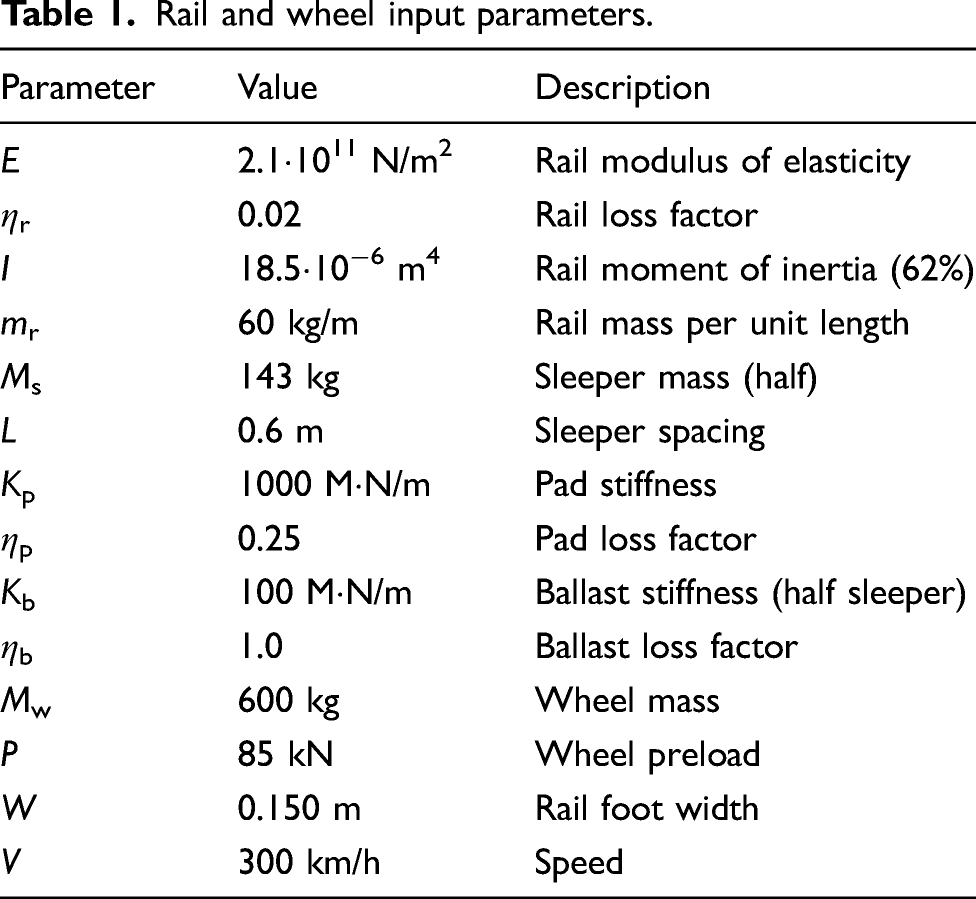
3.2. Input parameters

Table 1 shows values of input parameters used for the calculations. Stiff pads are assumed, with a stiffness value of 1000 M·N/m. This is a high value but not unrealistic because the pad stiffness generally increases with frequency (Nordborg and Verhelst, 2019) and load. In Germany, the most commonly used rail pad has a dynamic stiffness higher than 1000 M·N/m. The rail moment of inertia has been chosen to 62% of the nominal value. The ballast stiffness value regards half a sleeper. The wheel preload includes the wheel mass. In the time-domain model, non-linear Hertzian contact mechanics determines the value of the contact spring stiffness; in the frequency-domain model, the Hertzian contact spring stiffness is linearized. The rail surface roughness level used is the one for a rather rough rail; the TSI (the European railway standard Technical Specifications for Interoperability) limits plus 3 dB. The speed is 300 km/h for all calculations in this study.

Table 1.

Rail and wheel input parameters.

Parameter	Value	Description
E	2.1⋅10¹¹ N/m²	Rail modulus of elasticity
η _r	0.02	Rail loss factor
I	18.5⋅10⁻⁶ m⁴	Rail moment of inertia (62%)
m _r	60 kg/m	Rail mass per unit length
M _s	143 kg	Sleeper mass (half)
L	0.6 m	Sleeper spacing
K _p	1000 M·N/m	Pad stiffness
η _p	0.25	Pad loss factor
K _b	100 M·N/m	Ballast stiffness (half sleeper)
η _b	1.0	Ballast loss factor
M _w	600 kg	Wheel mass
P	85 kN	Wheel preload
W	0.150 m	Rail foot width
V	300 km/h	Speed

3.3. Rail/wheel Green’s functions

For the rail, point (Figure 2) and transfer FRFs (receptances) are needed to construct the moving impulse response function (Figure 3) and the moving FRF (Figure 4). Inverse Fourier transforms yield the moving impulse response function in the time domain (Nordborg, 2002) and transforming back again to the frequency domain, the moving FRF. It may be interesting to note, that the force point is not fixed to any particular position on the rail, but it is moving in the x-direction along the rail surface.

Figure 2.

Rail receptance (magnitude) (colour online). The upper curve shows the receptance between two sleepers and the lower on a sleeper position.

Figure 3.

Moving impulse response function of the rail. The rail is hit between two sleepers. The plot shows the impulse response in the point moving with the forward velocity v = 300 km/h along the rail surface.

Figure 4.

Moving rail receptance (magnitude). The rail is excited by a force moving with the forward velocity v = 300 km/h over the rail surface.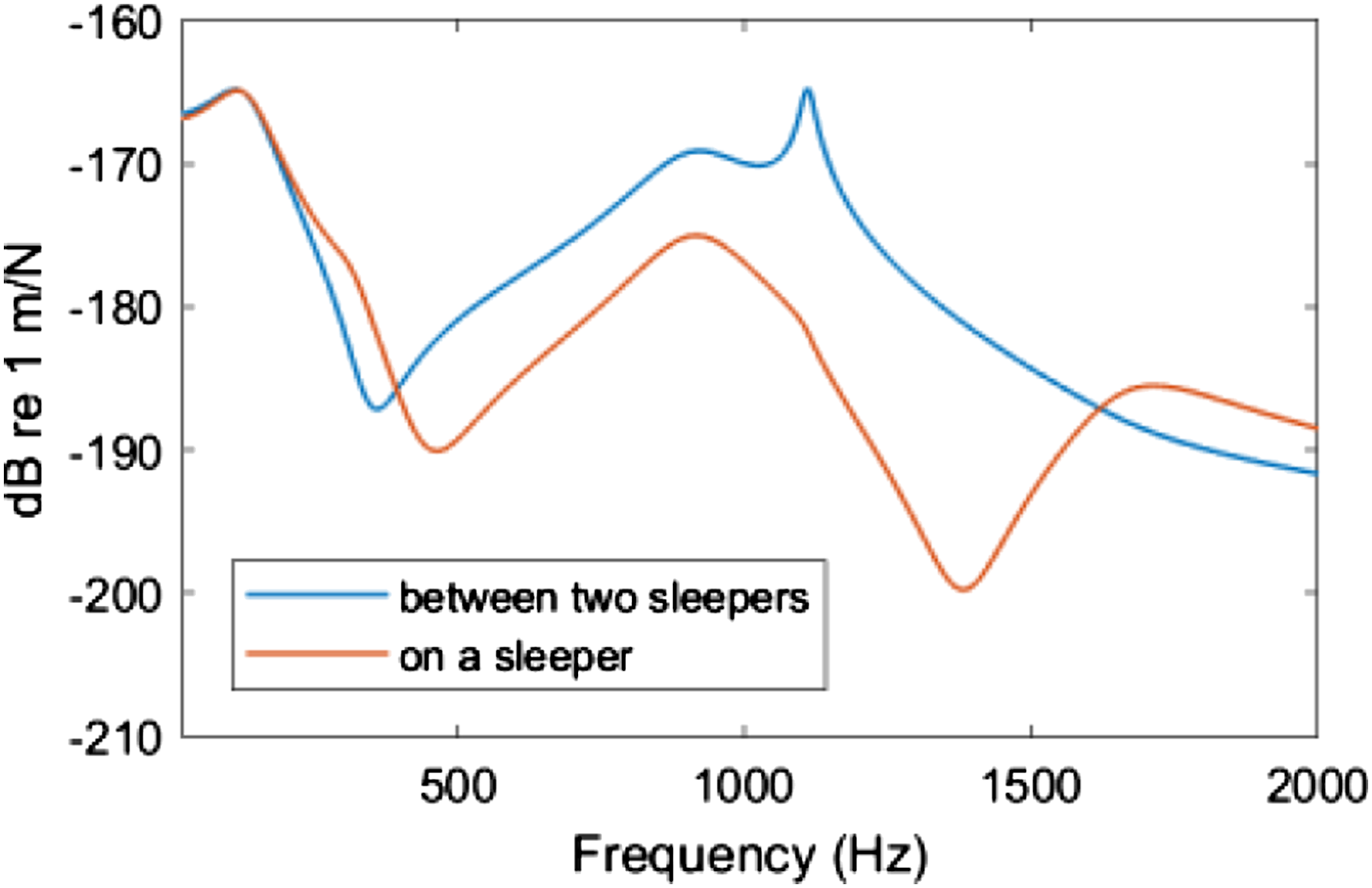

For the wheel, as for the rail, we need the moving (or rotating) impulse response function, in the rail/wheel contact point rotating around the perimeter. The same calculation scheme as for the rail is used, but a finite element model of the wheel yields the input and transfers FRFs in the radial direction (Nordborg and Kohrs, 2015). Using these functions, inverse Fourier transforms then generate the rotating impulse response function in the time domain (Figure 5). Fourier transforming the rotating impulse response function then generates the rotating FRF in the frequency domain (Figure 6).

Figure 5.

Rotating impulse response function of the wheel in the radial direction. The wheel is hit radially. The plot shows the radial impulse response in the point moving (rotating) around the wheel perimeter with the rotational velocity v = 300 km/h.

Figure 6.

Rotating wheel receptance in the radial direction. The wheel is excited by a force moving (rotating) around the wheel perimeter with the rotational velocity v = 300 km/h. For comparison, the stationary (non-rotating) point receptance is also shown.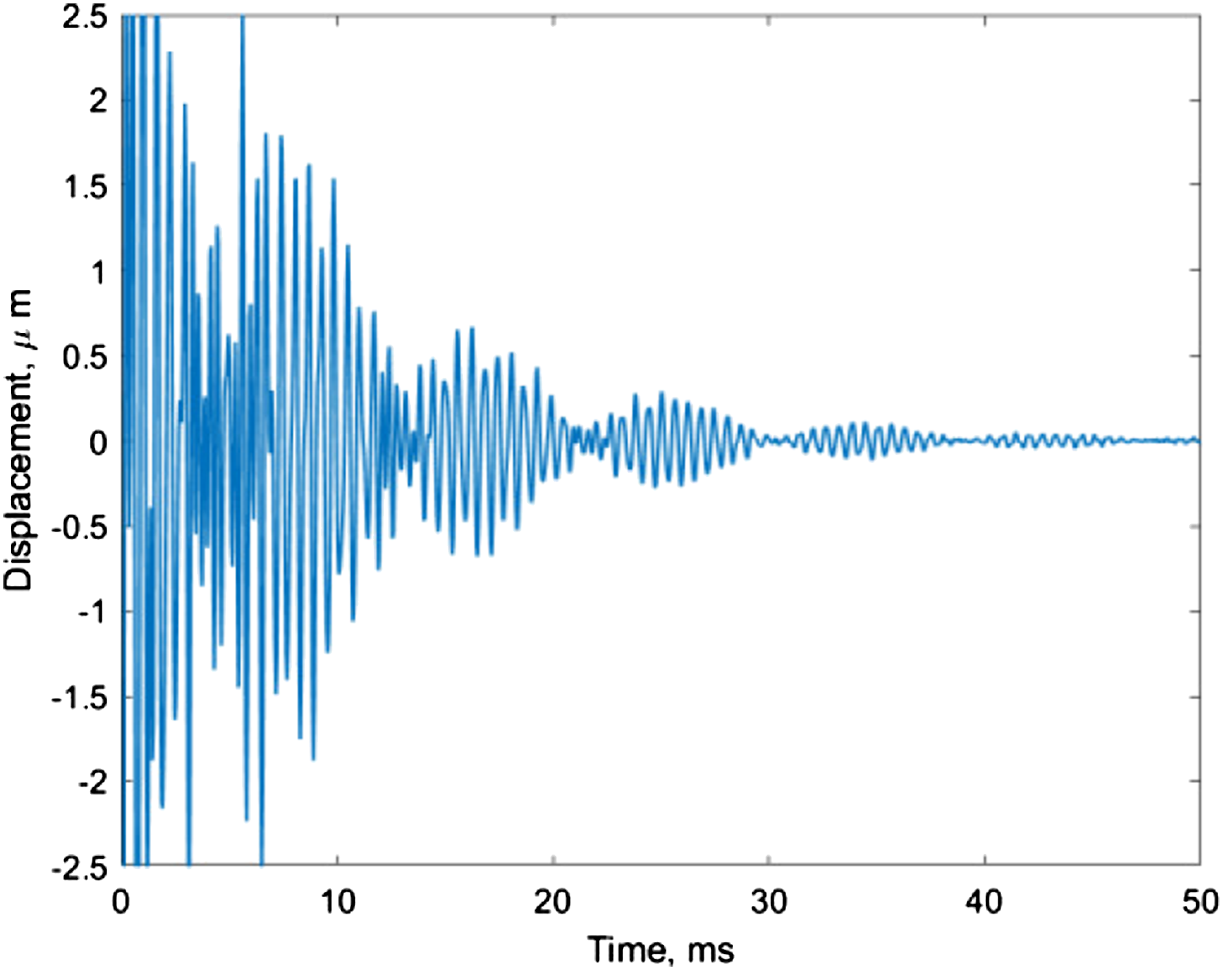

3.4. Rail/wheel interaction contact force: smooth rail surface.

In the first calculation example, a wheel rolling over a perfectly smooth rail is simulated. The rail/wheel contact force spectrum is shown in Figure 7. Also shown are spectra for a wheel rolling on a rail with a roughness spectrum 3 dB above the TSI limit and 10 dB below that.

Figure 7.

Rail/wheel interaction contact force when the rail surface is perfectly smooth −200 dB. Also shown are contact force spectra when the rail has a roughness level of Technical Specifications for Interoperability + 3 dB, and 10 dB below that. (colour online).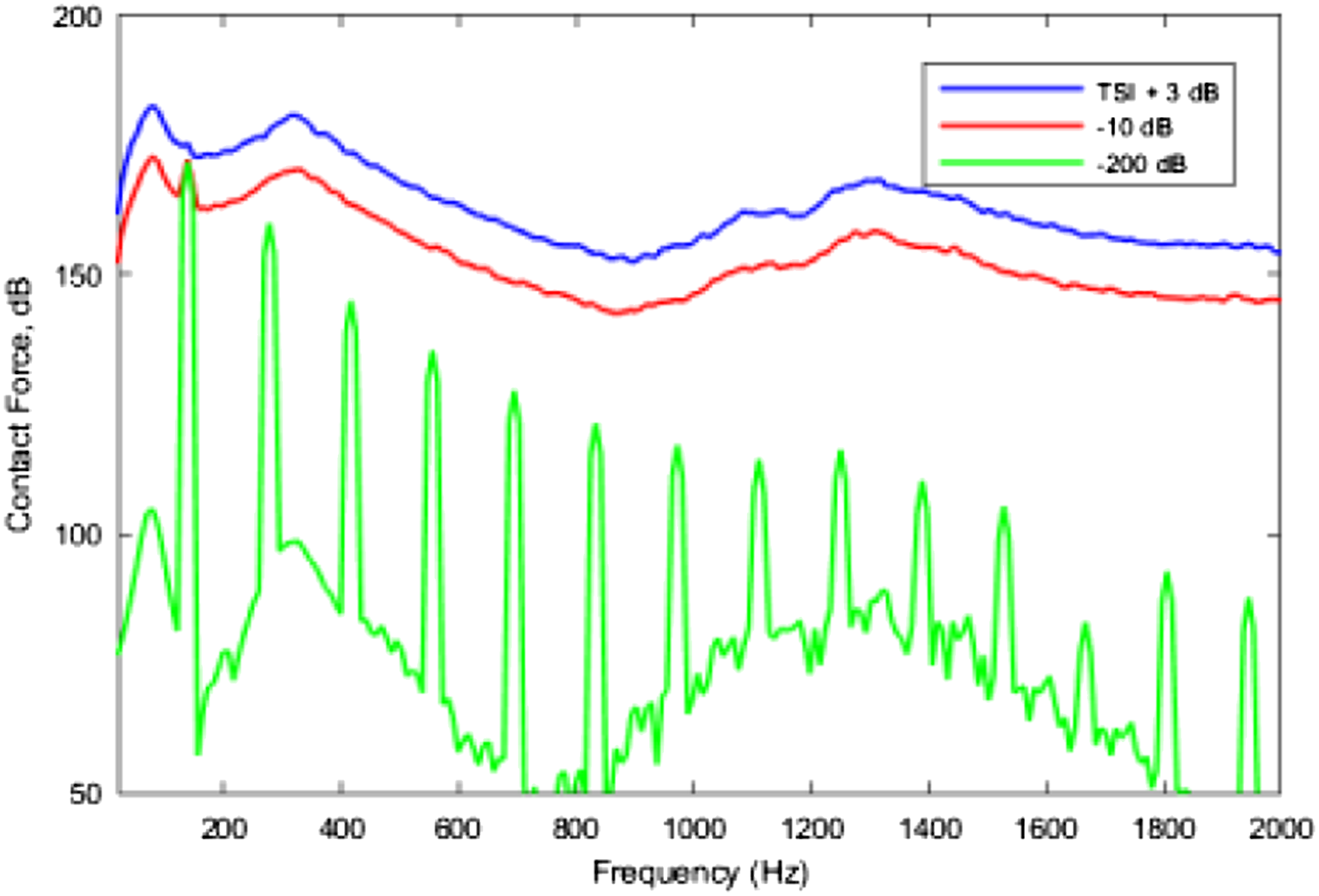

3.5. Rail/wheel interaction and rolling noise generation: rough rail surface

When the wheel rolls over the rail, the contact force f excites the rail and wheel into vibration, y_r, equation (5), and y_w, equation (6). As a consequence, the rail radiates noise W equation (9). Plots of spectra of the contact force and rail and wheel vibrations are shown in Figures 8 and 9. The plot in Figure 10 shows rail noise radiation. The time-domain model developed in this study is compared with the frequency-domain model (Nordborg and Koh, 2016). The interpretation of the plots is discussed in the next section.

Figure 8.

Contact force spectrum for time- (thick line) and frequency-domain (thin line) models (Nordborg and Koh, 2016). The frequency domain model has the same rail/wheel parameters as the time-domain model, but the rail/wheel interaction force is only a function of the roughness spectrum and the stationary point receptances of rail and wheel.

Figure 9.

Rail and wheel response vibration levels for the time-domain model (thick line) and the frequency-domain model (thin line) (colour online).

Figure 10.

Sound power level spectrum (narrow bands) of rail noise radiation for the time-domain model developed in this study and for the frequency-domain model (Nordborg and Koh, 2016).

4. Discussion

4.1. Rail/wheel Green’s functions

The plot of the vertical rail point receptance (Figure 2) shows three maxima caused by system resonances: the first caused by the vibration of the mass of the rail and sleepers on the ballast stiffness, the second caused by vibrations of the rail mass on the pad stiffness and the third, distinct one around 1.1 kHz, is the pinned–pinned frequency, where the rail vibrates with a bending wavelength equal to two sleeper spans, with nodes at the sleeper positions. The calculated point receptance curves at midspan and on a sleeper position exhibit a striking resemblance with measured ones (Nordborg and Verhelst, 2019). The receptance through a sleeper span varies substantially due to the stiff pads, with consequences for rolling noise generation, as discussed below. The moving impulse response function of the rail (Figure 3) contains a clearly visible contribution of the pinned–pinned frequency, superimposed on the lower frequency vibrations caused by vibrations of rail and sleeper masses on pad and ballast stiffnesses. The forward velocity leads to a splitting of the pinned–pinned frequency (Nordborg, 2002) (Figure 4).

What is striking from the rotating impulse response function (Figure 5) and receptance plot (Figure 6) of the wheel is the beating of the vibration amplitude in the time domain and splitting of resonance peaks in the frequency domain. The distance between the two peaks corresponds to the rotational speed and wheel diameter.

In changing the dynamic behaviour of the wheel response, amplitude and frequency of the wheel resonances, it is important to include the rotation, in particular at high frequencies for high-speed trains. However, below 1500 Hz, where rail vibrations around the pinned–pinned frequency are important, the frequency response for the wheel is flat, where a lumped mass model of the wheel probably also would work fine.

4.2. Rail/wheel interaction and rolling noise generation

When the wheel rolls over a perfectly smooth rail, parametric excitation (Nordborg, 1998a, 2002) due to varying rail receptance through the sleeper spans gives rise to peaks at the sleeper-passing frequency f_s = v/l (around 140 Hz) with harmonics, dominating the contact force spectrum (Figure 7). This peak is also present in the contact force spectrum for a rail with surface roughnesses. There are broadband contributions to the excitation around frequencies where the rail/wheel system has resonances: wheel–ballast resonance, rail–pad–sleeper resonance and the pinned–pinned frequency. These results are obtained with the time-domain model. The frequency-domain model would yield no response at all for a wheel rolling over a perfectly smooth rail. Parametric excitation can be seen also in the spectra for the rough rails, as an increased contact force around the pinned–pinned frequency (just above 1 kHz).

At first glance at Figure 7, it appears as if the peaks at the sleeper-passing frequency f_s = v/l (around 140 Hz) with harmonics are the most important and interesting contribution of parametric excitation caused by the periodic track stiffness due to the periodic rail supports. This excitation at discrete frequencies has been thoroughly investigated in other studies, for example in Nordborg (1998a, 2002), but broadband parametric excitation has not been addressed before. However, in this study, we focus on broadband contributions to the excitation, which, for example can be seen in the plot for the perfectly smooth rail in the frequency region 800–1800 Hz. This excitation is also caused by the periodic rail stiffness – that is – it is an effect of parametric excitation. It cannot be modelled properly by a linear model in the frequency-domain model because the process is non-stationary. This is why the calculated contact force is about 10–15 dB higher for the time-domain model than for the frequency-domain model in this frequency region in Figure 8.

The frequency-domain model, not including parametric excitation, underpredicts the contact force and rail vibration levels below 1500 Hz (Figures 8 and 9). The error is around 10 dB in a broad region around the pinned–pinned frequency, which occurs at 1.1 kHz in these simulation calculations. The reason for the underprediction of rail vibration levels is that the frequency-domain model cannot include the effects of parametric excitation and the feedback coupling mechanism between wheel/rail response and contact force, which on the other hand, the time-domain model automatically does. Rail (and wheel) deflections (Figure 3 and 5) due to vibrational response to the excitation force have the same effect on the contact force as the surface roughnesses, in equation (7); so, they are effectively taking part in the excitation process. In this way, a feedback from response to excitation force arises. At the pinned–pinned frequency, the rail vibrates with large amplitudes. Through the feedback coupling, the pinned–pinned mode thus strongly takes part in the excitation around the pinned–pinned frequency, explaining the big difference in vibration levels obtained with the two different (time- and frequency-domain) models. Stiff pads make the pinned–pinned mode more pronounced and increase the modulation around the pinned–pinned frequency, which increases noise radiation (Nordborg, 1998a, 2002).

After having multiplied, the force level spectrum (Figure 8) with the ESD₁ of the rail, the sound power spectrum (equation (9) and Figure 10) is obtained. For the rail on stiff pads in this calculation example, the difference in noise radiation between the time- and the frequency-domain models is greater than 3 dB (after A-weighting) because the frequency-domain model fails to capture the effects of parametric excitation. However, other sources also contributing to wayside railway noise (e.g. lateral rail vibration and aeroacoustic noise) may reduce the importance of rail noise near the pinned–pinned frequency, in particular, given the high speed (300 km/h) used in the simulation calculations in this study. Nevertheless, in addition to rail surface roughnesses, parametric excitation and the feedback coupling mechanism between wheel/rail response and contact force can be important excitation mechanisms and should be accounted for.

5. Conclusion

When a railway wheel rolls over a perfectly smooth sleeper-supported rail, the rail and wheel are excited into vertical vibration. Parametric excitation and modulation due to varying rail receptance through the sleeper spans and interaction feedback coupling between rail/wheel response and contact force determine the excitation contact force spectrum. For a stiffly padded rail with surface roughnesses, these effects contribute to the total A-weighted rail/wheel rolling noise generation with amounts that cannot be neglected. A proper modelling requires a time-domain model.

Footnotes

Acknowledgements

Thanks to Torsten Kohrs, Bombardier Transportation, Hyoin Koh, Korea Railroad Research Institute and to Katja Stampka, Technische Univesität Berlin for help and support.

Declaration of conflicting interests

The authors declared no potential conflicts of interest with respect to the research, authorship and/or publication of this article.

Funding

The authors received no financial support for the research, authorship and/or publication of this article.

ORCID iD

Anders Nordborg

References

Dalenbring

(1995) A study of the effect of track parameter changes on vertical rail vibrations. Technical Report no TRITA-FKT 9506. Stockholm: Department of Vehicle Engineering, Kungl Tekniska Högskolan.

Klaus

(2019) Einfluss von Radparametern auf Rollgeräusche bei Schienenfahrzeugen. Master’s Thesis, Technische Universität Berlin, Germany.

Lundberg

Nordborg

Lopez Arteaga

(2016) The influence of surface roughness on the contact stiffness and the contact filter effect in nonlinear wheel-track interaction. Journal of Sound and Vibration 366: 429–446.

Mazilu

(2007) Green's functions for analysis of dynamic response of wheel/rail to vertical excitation. Journal of Sound and Vibration 306: 31–58.

Nayfeh

and Mook

(1979) Nonlinear Oscillations. New York: John Wiley & Sons.

Nordborg

(1998a) Vertical rail vibrations: pointforce excitation. Acta Acustica 84(2): 280–288.

Nordborg

(1998b) Vertical rail vibrations: parametric excitation. Acta Acustica 84(2): 289–300.

Nordborg

(1999) Rail/wheel parametric excitation: laboratory and field measurements. Acta Acustica 85(3): 355–365.

Nordborg

(2002) Wheel/rail noise generation due to nonlinear effects and parametric excitation. The Journal of the Acoustical Society of America 111(4): 1772–1781.

10.

Nordborg

Koh

(2016) Comparison of two different models describing railway noise generation and radiation. In: Inter-noise congress and conference proceedings, Hamburg, Germany. INCE.

11.

Nordborg

Kohrs

(2015) Ein Zeitbereichsmodell Zur Beschreibung der Rollgeräuschentstehung. In: DAGA congress and conference proceedings, Nurnberg, Germany.

12.

Nordborg

Verhelst

(2019) Validation and Comparison with Measurements at Infrabel of a Time Domain Model Describing Railway Noise Generation. In: IWRN13 congress and conference proceedings, Ghent, Belgium.

13.

Pieringer

(2014) A numerical investigation of curve squeal in the case of constant wheel/rail friction. Journal of Sound and Vibration 333: 4295–4313.

14.

Remington

(1987a) Wheel/rail rolling noise, I: theoretical analysis. The Journal of the Acoustical Society of America 81: 1805–1823.

15.

Remington

(1987b) Wheel/rail rolling noise, II: validation of the theory. The Journal of the Acoustical Society of America 81: 1824–1832.

16.

Sheng

Xiao

Zhang

(2016) The time domain moving green function of a railway track and its application to wheel-rail interactions. Journal of Sound and Vibration 377: 133–154.

17.

Thompson

(2009) Railway Noise and Vibration. Oxford: Elsevier.

18.

Thompson

(2004) On the parametric excitation of the wheel/track system. Journal of Sound and Vibration 278: 725–747.

19.

Thompson

(2006) On the rolling noise generation due to wheel/track parametric excitation. Journal of Sound and Vibration 293: 566–574.