H ∞ Control law for line of sight stabilization in two-axis gimbal system

Abstract

A two-axis gimbaled stabilization system in air vehicles must stabilize the line of sight of the payload toward a target against the external motion induced by air vehicle maneuvering and aerodynamic forces. The target tracking and pointing performances of the air vehicles are largely affected by air vehicle motion decoupling capability. In this work, the $H_{\infty}$ controller design is carried out for a two-axis gimbal system. The plant model is generated using experimental frequency response data and mathematical formulation of the system. The mixed sensitivity problem is posed and weighting functions are selected so that they not only fulfill all the design goals but also accommodate the modeling uncertainties. The stabilization loop is designed and implemented in digital signal processor-based hardware for only one axis (in azimuth).

Keywords

Line of sight gimbal system electro optic payload model uncertainty mixed sensitivity digital signal processor

1. Introduction

A stabilized platform is an electromechanical system was designed primarily to isolate a “payload” from its environment. The payload might be a forward-looking infrared receiver (FLIR), TV camera, Laser designator, missile seeker, or other active elements. The motion of the aircraft, missile, ship, or land vehicle, which carries the payload, determines the environment. The second objective of a stabilized platform is to “point” the payload in a given direction as it is operated in its environment as explained by Gawronski (2007) and Hong et al (2011). Therefore, the stabilization system is a mechanical interface between the sensor payload and the vehicle, which carries the payload. It consists of a mechanism, which enables the payload’s line of sight (LOS) orientation to be altered with respect to the vehicle orientation and a means for manipulating the mechanism so that the LOS is controlled in some desired manner.

The torque disturbances in the system can be due to bearing and motor friction, unbalanced aerodynamics, and vibration forces from onboard mechanisms. Lesser residual jitter on the LOS enables longer operating ranges. Figure 1 shows a typical stabilization loop in azimuth axis.

Figure 1.

Block diagram of stabilization loop in azimuth axis.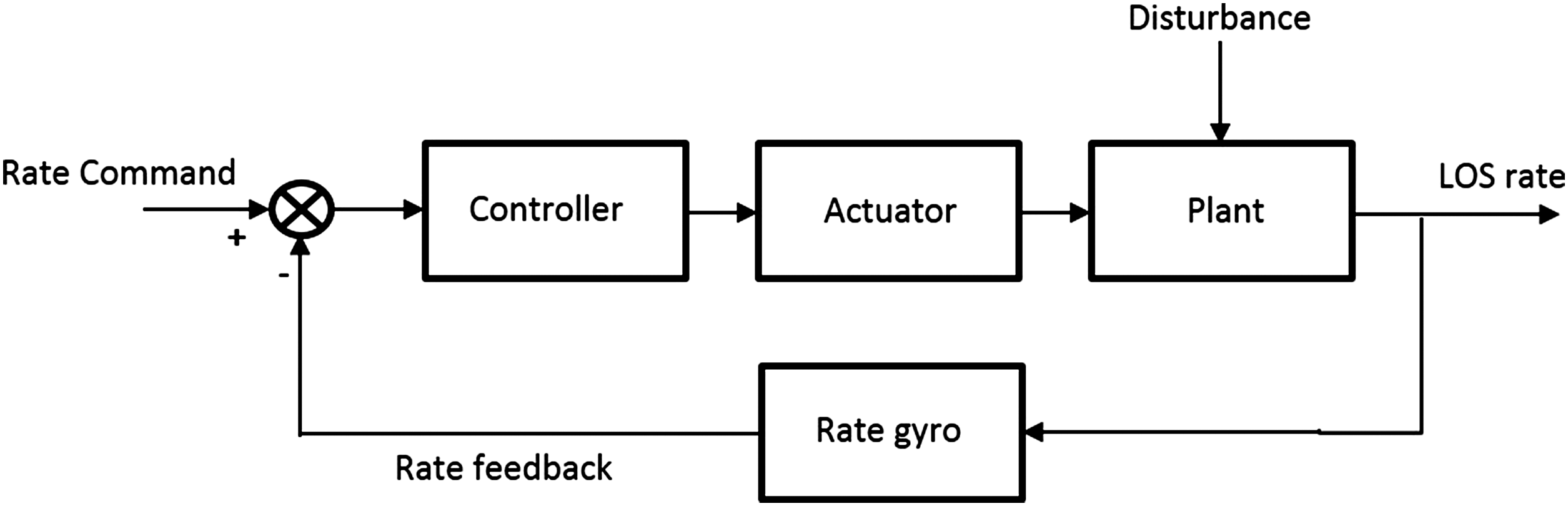

Several methods for LOS stabilization of gimbal system have been proposed in the literature. Abdo et al. (2014) constructed the azimuth and elevation axes stabilization loops with cross-coupling using a fuzzy PID-type controller. Wang et al. (2014) developed the FOPI controller for the LOS stabilization system with some nonlinearity and uncertainty. Toloei et al. (2016) developed the stabilization loop with DC motor, rate gyro, and inertia-utilizing model predictive control, and evaluated the performance of one-axis gimbal system in various conditions, considering the gimbal friction, mass imbalance, and disturbance torques. Fang. et al. (2015a, 2015b) used the neural network compensator and input–output feedback linearization to design an adaptive decoupling controller for three-axis gyro-stabilized platform. The nonlinearity and coupling are resolved by input–output feedback linearization, and the uncertainties & disturbances are estimated by the radial basis function neural networks. Ashok Kumar and Kanthalakshmi (2018) used weighted sensitivity approach to design optimal H infinity controller for an Inverted pendulum system by interatively varying performance weight function.

In this study, we carried out the modeling of two-axis gimbal system using experimental frequency response approach and mathematical formulation of the system. The $H_{\infty}$ control methodology (mixed sensitivity) is used to design the rate stabilization loop in azimuth axis to mainly cater for requirements such as uncertainty in the model and disturbance rejection. The $H_{\infty}$ control with mixed sensitivity design provides direct means of shaping the sensitivity $S (s)$ & complementary sensitivity functions $T (s)$ and in particular to tackle unstructured modeling uncertainties. The design specifications for robust stability and command following are met by appropriately designing the various weight functions.

The design specifications are:

Closed loop (−3 dB) bandwidth 25–30 Hz

Gain margin, >9 dB

Phase margin, >40 deg

Damping coefficient, 0.5–0.7

System should cater for disturbances up to 10 Hz

Command signals are typically up to 5 Hz

The rest of this study is organized as follows: Section 2 describes a mathematical modeling of two-axis gimbal system. Then, when having a state space model of the system, Section 3 describes the perturbed model; Section 4 explains the design of weight functions; and Section 5 describes design of the controller. Finally, the results from simulations will then be presented, compared, and concluded in Sections 6 and 7, respectively.

2. Model of two-axis gimbal system

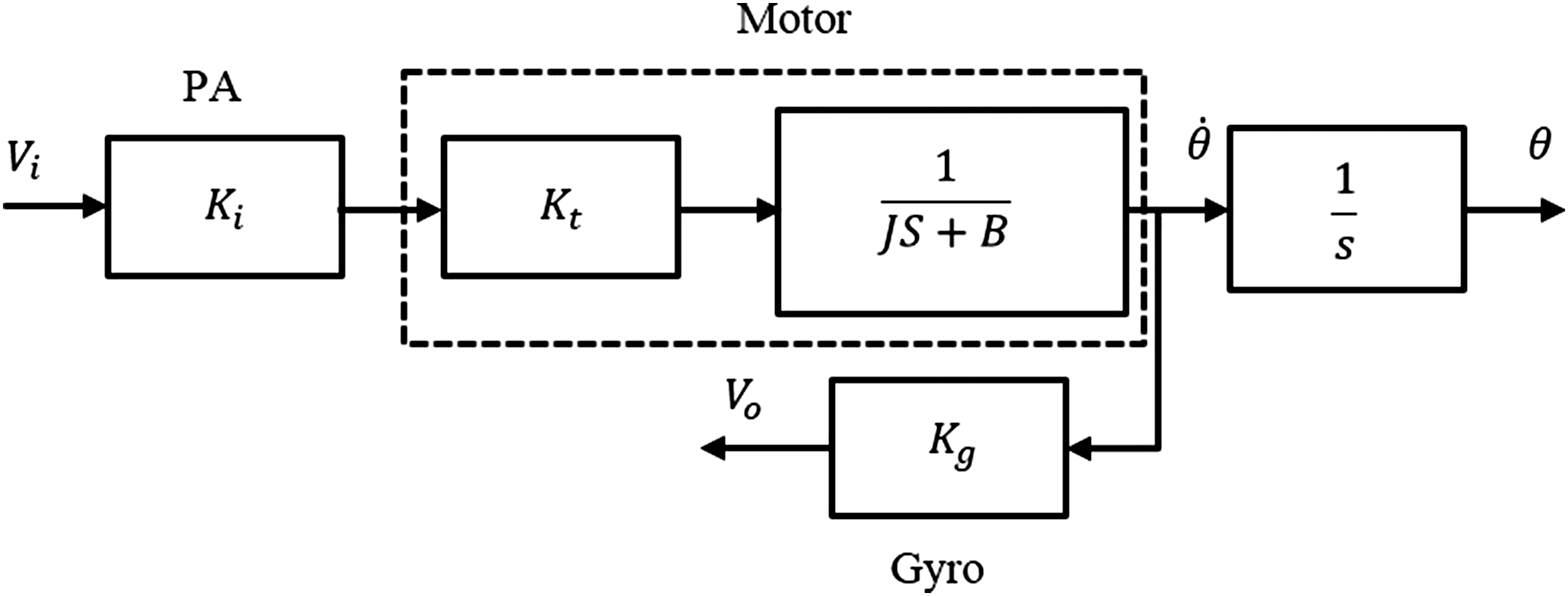
The two-axis gimbal system under consideration is an electromechanical system which consists of two power amplifiers and DC motors as actuators as shown in Figure 2. The power amplifiers are operated in current mode and the DC motors are permanent magnet type. The payloads (FLIR and TV camera) are fixed in the innermost gimbal, that is, elevation. The rate of the gimbal is sensed by high-performance rate gyros in both the axes. The block diagram of the gimbal system in azimuth axis is illustrated in Figure 3. Because the gimbal system has mechanically high precision and mechanical axes of the gimbal are truly orthogonal, cross-coupling between the two axes are negligible.

Figure 2.

The two-axis gimbal configuration.

Figure 3.

The block diagram of gimbal system in azimuth axis. Where, 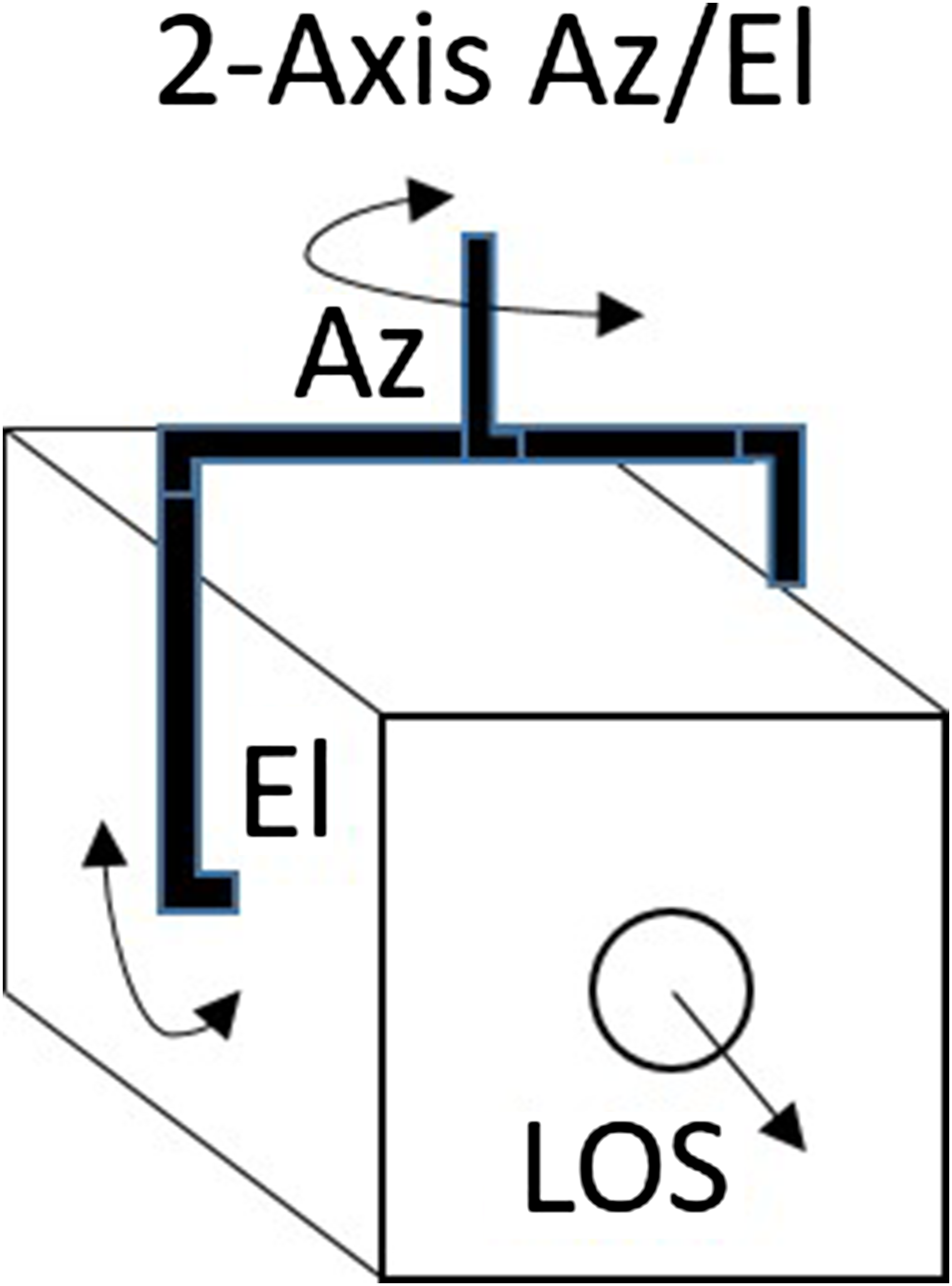$K_{i} =$ current amplifier gain (amp/volt), $K_{t} =$ motor torque constant (N·m/amp), $K_{g} =$ gyro scale factor (volt/deg/s), $J =$ gimbal moment of inertia $(kg \cdot m^{2})$ , and $B =$ viscous friction coefficient (N·m/rad/s).

The physical plant open loop frequency response data for the azimuth channel were obtained experimentally using the dynamic signal analyzer. The data used for the modeling are obtained by taking average of 10 datasets. The frequency response experimental setup is illustrated in Figure 4.

Figure 4.

Frequency response experimental setup.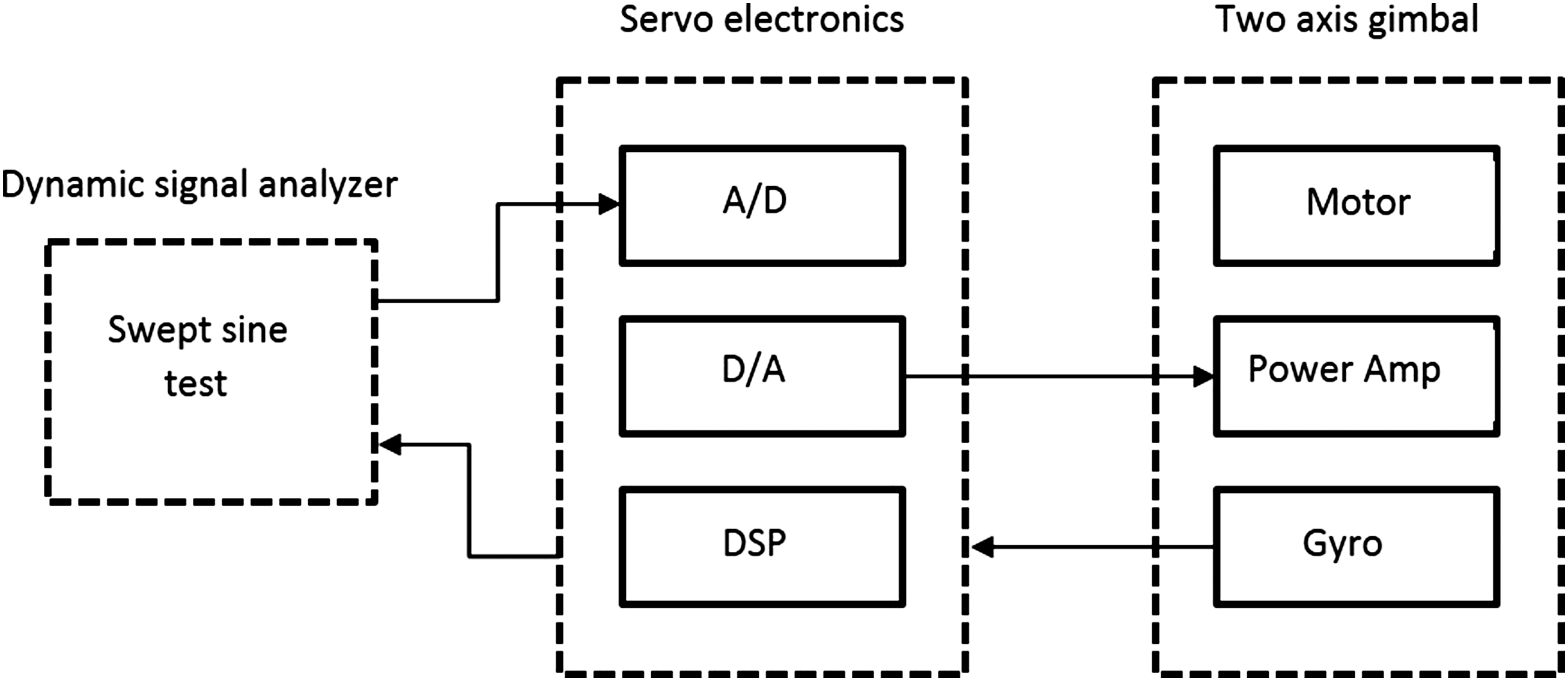

The frequency response data from dynamic signal analyser are shown in the form of a Bode plot. An eighth-order model was fitted to this experimental data, and further, a second-order model is obtained by reducing it. Figure 5 represents experimental frequency response, curve-fitted model (eighth order), and reduced model (second order).

Figure 5.

Bode plots of experimental data, eighth- and second-order models.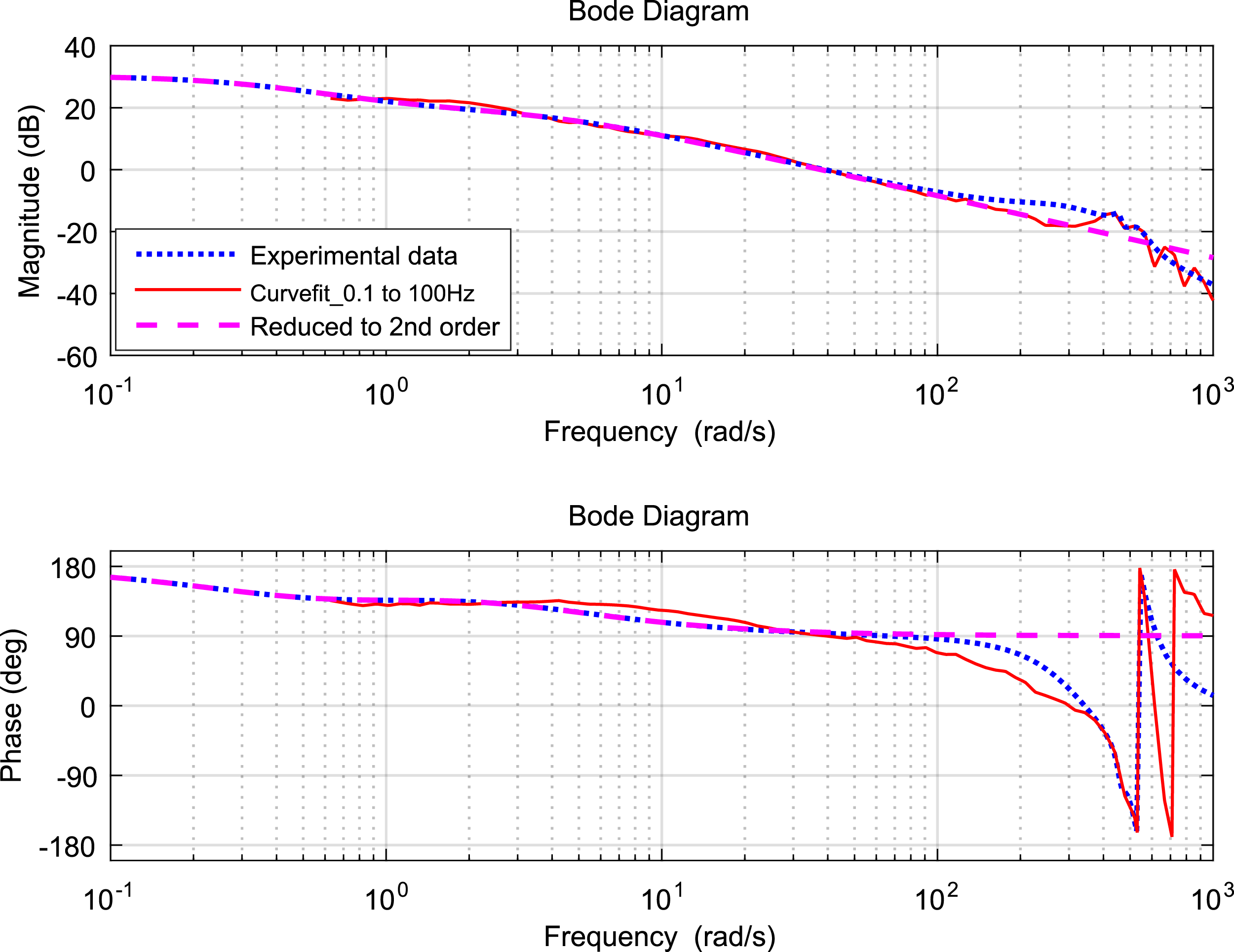

The state space representation of the second-order plant model is given in equations (1)–(5)

2 nd order TF = \frac{- 37.96 s - 40.67}{s^{2} + 4.376 s + 1.255}

(1)

[\begin{matrix} {\dot{x}}_{1} \\ {\dot{x}}_{2} \end{matrix}] = [\begin{matrix} - 0.7174 & - 1.171 \\ - 1.171 & - 3.659 \end{matrix}] [\begin{matrix} x_{1} \\ x_{2} \end{matrix}] + [\begin{matrix} - 4.435 \\ - 4.278 \end{matrix}] u

(2)

y = [\begin{matrix} 4.435 & 4.278 \end{matrix}] [\begin{matrix} x_{1} \\ x_{2} \end{matrix}] + [0] u

(3)

Alternatively

[\begin{matrix} {\dot{x}}_{1} \\ {\dot{x}}_{2} \end{matrix}] = [\begin{matrix} - 4.376 & 1 \\ - 1.255 & 0 \end{matrix}] [\begin{matrix} x_{1} \\ x_{2} \end{matrix}] + [\begin{matrix} - 37.96 \\ - 40.67 \end{matrix}] u

(4)

y = [\begin{matrix} 1 & 0 \end{matrix}] [\begin{matrix} x_{1} \\ x_{2} \end{matrix}] + [0] u

(5)

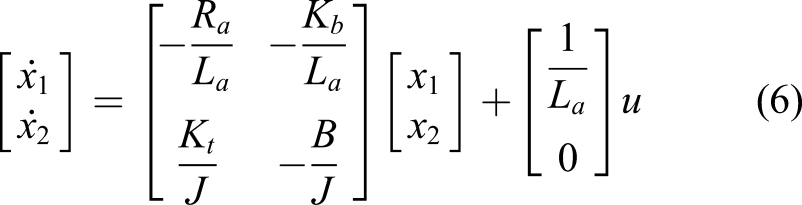
By referring to Figure 3, the typical mathematical model for the two-axis gimbal system in azimuth alone can be derived as in equations (6) and (7)

[\begin{matrix} {\dot{x}}_{1} \\ {\dot{x}}_{2} \end{matrix}] = [\begin{matrix} - \frac{R_{a}}{L_{a}} & - \frac{K_{b}}{L_{a}} \\ \frac{K_{t}}{J} & - \frac{B}{J} \end{matrix}] [\begin{matrix} x_{1} \\ x_{2} \end{matrix}] + [\begin{matrix} \frac{1}{L_{a}} \\ 0 \end{matrix}] u

(6)

y = [\begin{matrix} 0 & 1 \end{matrix}] [\begin{matrix} x_{1} \\ x_{2} \end{matrix}] + [0] u

(7)

where

x_{1} = i_{a} =

armature current,

x_{2}

ω

=

\dot{θ}

= angular rate, and θ = angular position.

After substituting the nominal parameters from Table 1

[\begin{matrix} {\dot{x}}_{1} \\ {\dot{x}}_{2} \end{matrix}] = [\begin{matrix} - 2 e 5 & 1 \\ - 6.341 e 4 & 0 \end{matrix}] [\begin{matrix} x_{1} \\ x_{2} \end{matrix}] + [\begin{matrix} 0 \\ 7.915 e 6 \end{matrix}] u

(8)

y = [\begin{matrix} 1 & 0 \end{matrix}] [\begin{matrix} x_{1} \\ x_{2} \end{matrix}] + [0] u

(9)

Table 1.

Nominal parameters of plant.

Symbol	Description	Value/unit
$R_{a}$	Armature resistance	$2 Ω$
$L_{a}$	Armature inductance	$0.0001 H$
$K_{b}$	Back electromotive force	$0.0001 volt / rad / s$
$K_{t}$	Torque constant	$0.43 N \cdot m / A$
$B$	Viscous friction coefficient	$0.031 N \cdot m / rad / s$
$J$	Rotor inertia	$0.09779 kg \cdot m^{2}$

Both experimental and mathematical models of second order are plotted in Figure 6.

Figure 6.

Bode plots of experimental and mathematical models.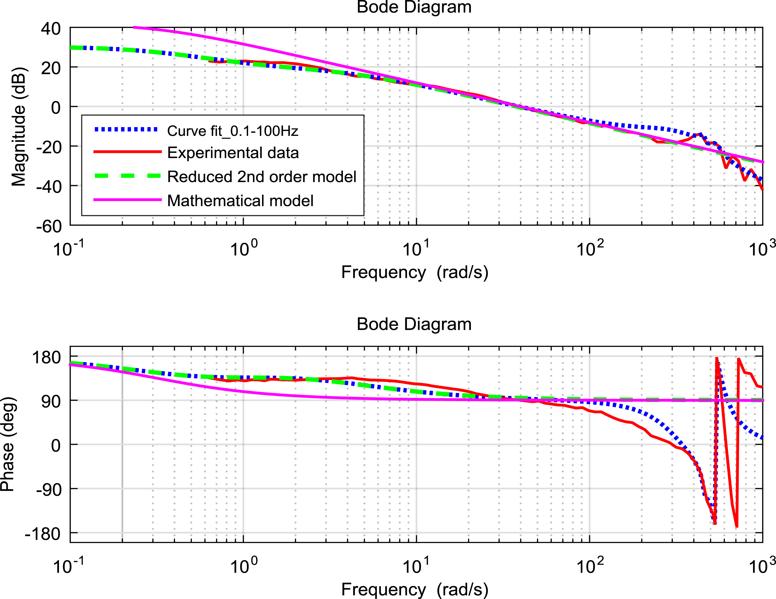

From Figure 6, it is concluded that the second-order mathematical model is sufficiently representing the plant at the low-frequency region. Therefore, this second-order model can be used to design the controller.

3. Perturbation model

The response of perturbed and nominal models are shown below in Figures 7 and 8.

Figure 7.

Bode plots of nominal and perturbed models.

Figure 8.

Step response of nominal and perturbed models.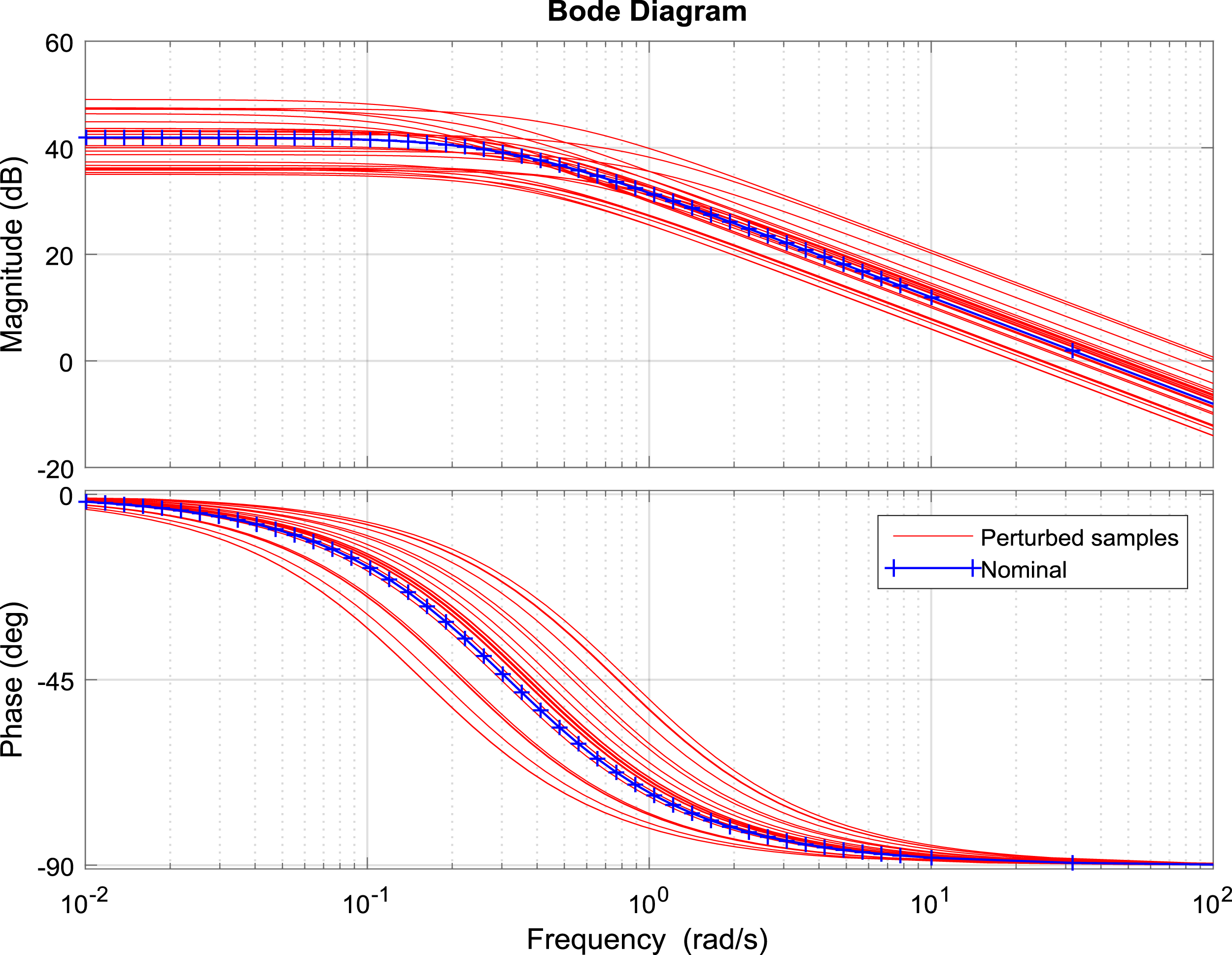

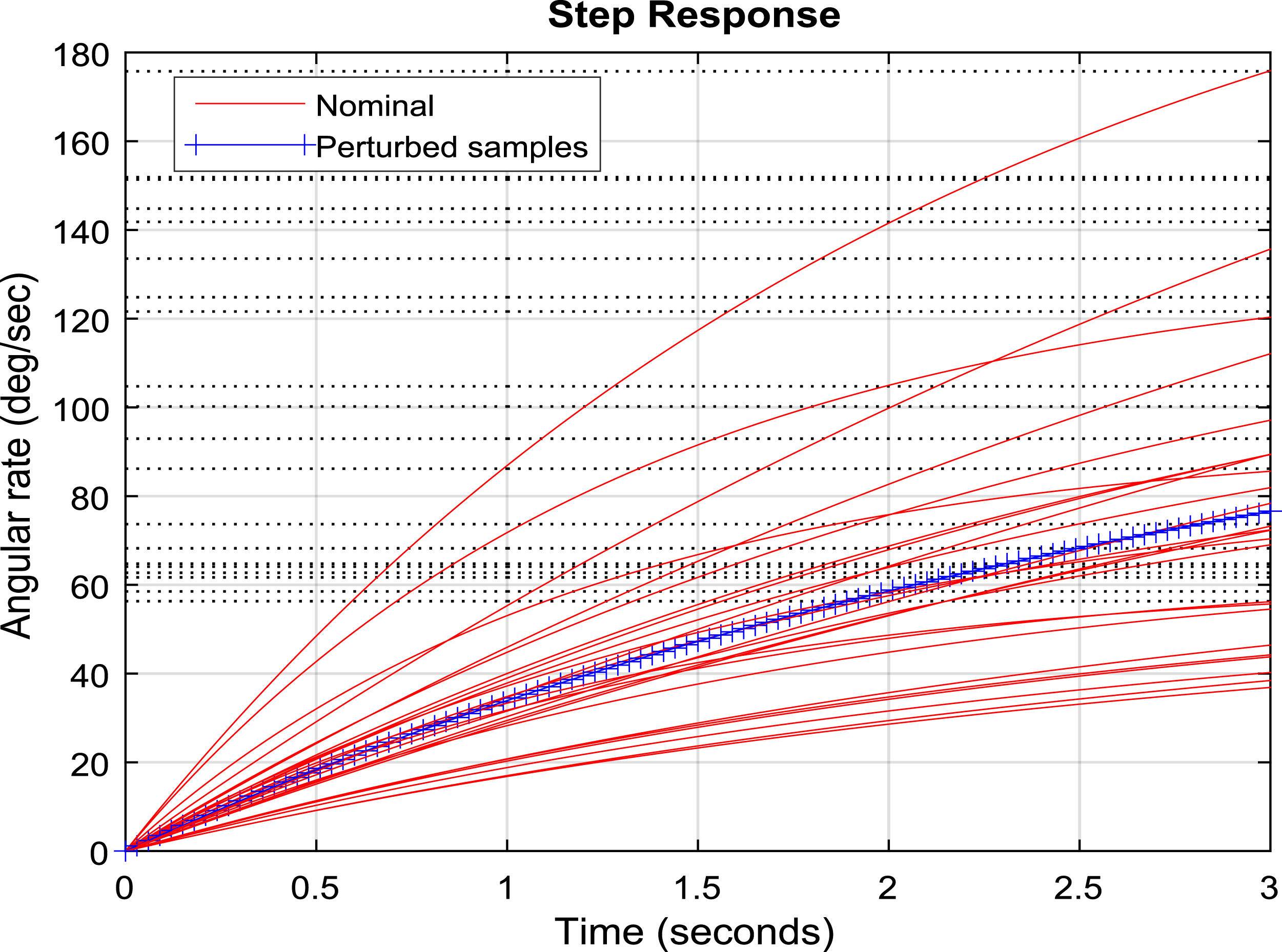
Perturbed models are generated by referring to the nominal model of the plant from equations (8) and (9), and from the nominal parameters of two-axis gimbal system from Table 1, the uncertainty is introduced in viscous friction coefficient $(B)$ , moment of inertia $(J)$ , and torque constant $(K_{t})$ with variability (−50,50)%.

4. $H_{\infty}$ Control methodology

The standard $H_{\infty}$ configuration is shown in Figure 9 (Skogestad and Postlethwaite, 2007). $P$ is the generalized plant (contains the plant, weights, and uncertainties if any), K is the controller (it internally stabilizes the plant, $P$ ), $x$ represents state vector, $w$ represents disturbance, $u$ represents control inputs and $v$ represents measured output variables, and $z$ represents controlled output variables.

\begin{array}{l} \dot{x} = A x + B_{1} w + B_{2} u \\ z = C_{1} x + D_{11} w + D_{12} u \\ v = C_{2} x + D_{21} w + D_{22} u \end{array}

(10)

P (s) = [\begin{matrix} P_{11} & P_{12} \\ P_{21} & P_{22} \end{matrix}] = [\begin{matrix} A & B_{1} & B_{2} \\ C_{1} & D_{11} & D_{12} \\ C_{2} & D_{21} & D_{22} \end{matrix}]

(11)

\begin{array}{l} {T_{z w} (s) |}_{u = 0} = P_{11} (s) = C_{1} {(S I - A)}^{- 1} B_{1} + D_{11} \\ {T_{v w} (s) |}_{u = 0} = P_{21} (s) = C_{2} {(S I - A)}^{- 1} B_{1} + D_{21} \\ {T_{z u} (s) |}_{w = 0} = P_{12} (s) = C_{1} {(S I - A)}^{- 1} B_{2} + D_{12} \\ {T_{v u} (s) |}_{w = 0} = P_{22} (s) = C_{2} {(S I - A)}^{- 1} B_{2} + D_{22} \end{array}

(12)

Figure 9.

The standard $H_{\infty}$ configuration.

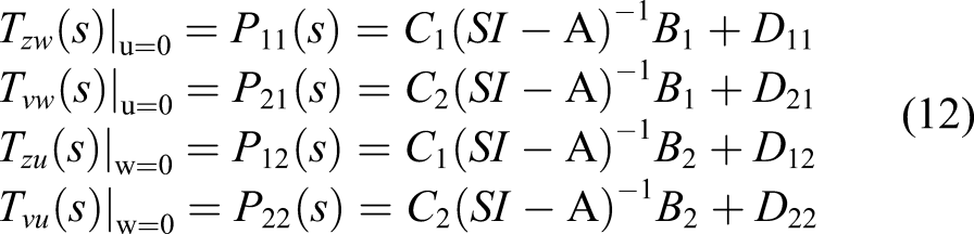
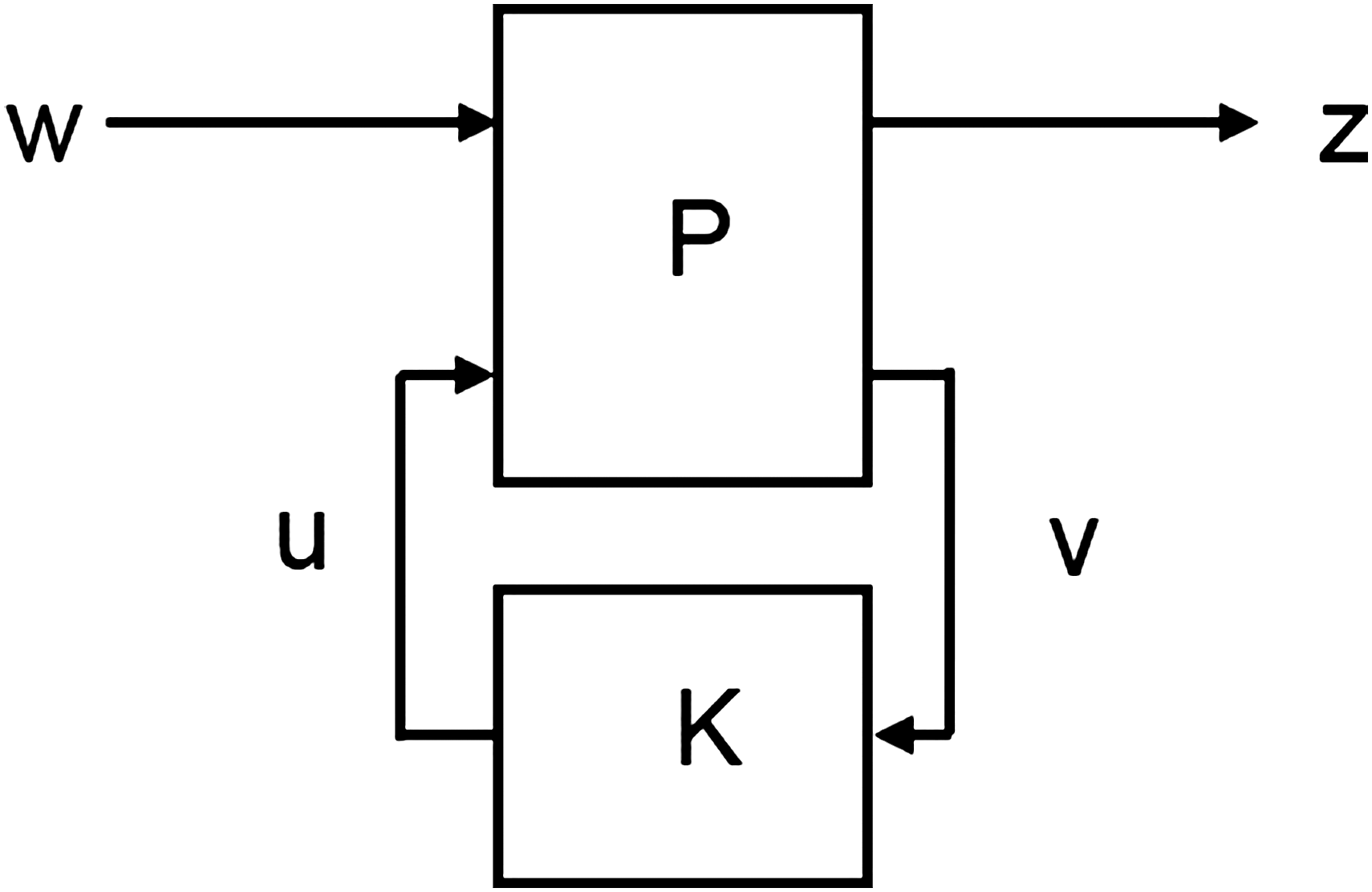
The closed-loop transfer function is given by

T_{z w} = F_{l} (P, K) = \frac{Z (S)}{W (S)} = P_{11} + P_{12} K {(I - P_{22} K)}^{- 1} P_{21}

(13)

where

F_{l} (P, K)

is referred to as a lower linear fractional transformation (Skogestad and Postlethwaite, 2007)

\underset{K (s) stabilising}{minimize} {‖ F_{l} (P (s), K (s)) ‖}_{H_{\infty}}

(14)

The optimal $H_{\infty}$ Control problem is to find all admissible controllers K(s) such that the transfer function from $w$ to $z$ , ${‖ T_{z w} ‖}_{\infty}$ is minimized (i.e., ${‖ T_{z w} ‖}_{\infty} < γ > 0$ ). By solving the two algebraic Ricatti equations (AREs) (Balas et al., 2008; Kwakernaak 1993) as shown in equations (15) and (17), the controller and estimator gains can be computed and are given in equations (16) and (20), respectively

X_{\infty} : R i c [\begin{matrix} A B_{2} {\bar{D}}_{12} D_{12} C_{1} & B_{2} {\bar{D}}_{12} B_{2}^{T} - γ^{- 2} B_{1} B_{1}^{T} \\ - {\bar{C}}_{1}^{T} {\bar{C}}_{1} & {(A - B_{2} {\bar{D}}_{12} {\bar{D}}_{12}^{T} C_{1})}^{T} \end{matrix}]

(15)

where

γ

is a positive quantity and

{(D_{12}^{T} D_{12})}^{- 1} = {\bar{D}}_{12}

and

\bar{C_{1}} = (I - D_{12} {\bar{D}}_{12} D_{12}^{T}) C_{1}

K_{c} = {\bar{D}}_{12} (B_{2}^{T} X_{\infty} + D_{12}^{T} C_{1})

(16)

Y_{\infty} : R i c [\begin{matrix} {(A - B_{1} D_{21}^{T} {\bar{D}}_{21} C_{2})}^{T} & - (C_{2}^{T} {\bar{D}}_{21} C_{2} - γ^{- 2} C_{1}^{T} C_{1}) \\ - {\bar{B}}_{1} {\bar{B}}_{1}^{T} & - (A - B_{1} D_{21}^{T} {\bar{D}}_{21} C_{2}) \end{matrix}]

(17)

where

{\bar{D}}_{12} = {(D_{21}^{T} D_{21})}^{- 1}

and

\bar{B_{1}} = (I - D_{21}^{T} {\bar{D}}_{21} D_{21}) B_{1}

K_{e} = (Y_{\infty} C_{2}^{T} + B_{1} D_{21}^{T}) {\bar{D}}_{21}

(18)

Z_{\infty} = {(I - γ^{- 2} Y_{\infty} X_{\infty})}^{- 1}

(19)

K_{L} = Z_{\infty} K_{e}

(20)

The estimator equation is given as

\dot{\hat{X}} = A \hat{X} (t) + B_{1} \hat{w} (t) + B_{2} u (t) + K_{L} (y (t) - \hat{y} (t))

(21)

where

\hat{w} (t) = γ^{- 2} B_{1}^{T} X_{\infty} \hat{X} (t)

and

\hat{y} (t) = C_{2} \hat{X} (t) + D_{21} \hat{w} (t)

K (s) : [\begin{matrix} (A - B_{2} K_{c} - K_{L} C_{2} - γ^{- 2} (B_{1} B_{1}^{T} - K_{L} D_{21} B_{1}^{T}) X_{\infty} & K_{L} \\ - K_{c} & 0 \end{matrix}]

(22)

ρ (X_{\infty}, Y_{\infty}) < γ^{2}

(23)

where

ρ

is the spectral radius

(ρ (A) = {max}_{i} | λ_{i} (A) |)

as explained by McFarlane and Glover (1992).

The value of $γ$ represents the accuracy factor within which the loop gain approaches the desired value as explained in Davidson and Ushakumari (2016).

4.1. Mixed sensitivity design

The performance objectives are as follows:

Weighted sensitivity (tracking error and bandwidth)

{‖ W_{P} (s) S (s) ‖}_{H_{\infty}} \leq 1

(24)

2. Actuation limits

{‖ W_{u} (s) K (s) S (s) ‖}_{H_{\infty}} \leq 1

(25)

3. Complementary sensitivity (reduced sensitivity to noise and uncertainty at high frequencies)

{‖ W_{T} (s) T (s) ‖}_{H_{\infty}} \leq 1

(26)

The bounded 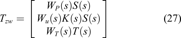$\bar{σ} (S)$ (for performance), $\bar{σ} (T)$ (for robustness and to avoid sensitivity to noise), and $\bar{σ} (K S)$ (to penalize large inputs) requirements are combined and represented as a stacked $H_{\infty}$ problem, that is, stacked S/T/KS problem

T_{z w} = [\begin{matrix} W_{P} (s) S (s) \\ W_{u} (s) K (s) S (s) \\ W_{T} (s) T (s) \end{matrix}]

(27)

where

W_{P} (s), W_{T} (s)

, and

W_{u} (s)

are the frequency-dependent weighting functions. The mixed sensitivity problem formulation is given in Section 5

{‖ T_{z w} ‖}_{H_{\infty}} = \sup_{ω} \bar{σ} (T_{z w} (j ω)) \leq γ

(28)

where

\sup_{ω} \bar{σ} (T_{z w} (j ω)) = \sup_{ω} \bar{σ} \sqrt{{| W_{P} S |}^{2} + {| W_{u} K S |}^{2} + {| W_{T} T |}^{2}}

The transfer function matrix $(P (s))$ , between $z$ and $w$ , $T_{z w}$ in equation (27) and Figure 9, the standard $H_{\infty}$ configuration can be represented by the block diagram in Figure 10 (Gu et al., 2005; Mackenroth 2010). Here, $w$ represents a reference command or disturbance entering at the output and $z$ consists of the weighted input $z 2 = W_{u} u$ , the weighted output $z 3 = W_{T} y$ , and the weighted control error $z 1 = W_{p} (y - r)$ . $where w = [\begin{matrix} w_{1} \\ w_{2} \\ w_{3} \end{matrix}] = [\begin{matrix} d \\ r \\ n \end{matrix}]; e = y - r; v = r - y_{m} = r - y - n$ ; $d, r, n, y & y_{m}$ are disturbance, command, noise, actual output, and measured output, respectively.

Figure 10.

Equivalent representation of the standard 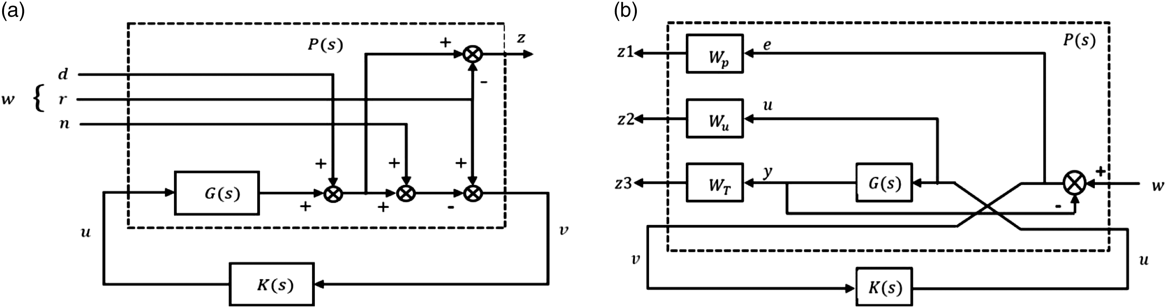$H_{\infty}$ configuration.

In $H_{\infty}$ synthesis problems, the weighting functions are very important. They should be selected in such a way that all design requirements are satisfied. After a selection of suitable weights, the algorithm given in Section 4 can be implemented, and after few iterations on $γ$ , an optimal controller is obtained.

5. $H_{\infty}$ Controller design

The key factor in the $H_{\infty}$ control design is the selection of the weighting functions. Weight on the sensitivity function, $W_{p}$ , is selected to satisfy 31 dB up to 1 Hz, and then, at least equal to 21 dB up to 3 Hz to meet the disturbance attenuation specifications for this plant. The gains are calculated to reject the worst-case disturbance around 10 Hz (by calculating the ratio of the input disturbance rate and the allowable residual jitter of the LOS rate at that frequency). And bandwidth is targeted such that the sensitivity function of 0 dB crossover occurs at 27 Hz. Also, maximum peak of the sensitivity function, $M_{s}$ chosen to be less than two and steady state error chosen as $5 \times 10^{- 6}$ to avoid pure integrator in the controller.

W_{p} = \frac{0.47 s^{3} + 437.3 s^{2} + 1.324 e 5 s + 1.304 e 7}{s^{3} + 385.8 s^{2} + 3.393 e 4 s + 33.93}

(29)

The frequency response plots of $W_{P}^{- 1}$ and $S$ are shown in Figure 11(a). The frequency response plots of $W_{T}^{- 1}$ and $T$ are shown in Figure 11(b) below.

Figure 11.

Bode magnitude plots of weight functions and resultant sensitivity and complementary functions. (a) Bode magnitude plots of 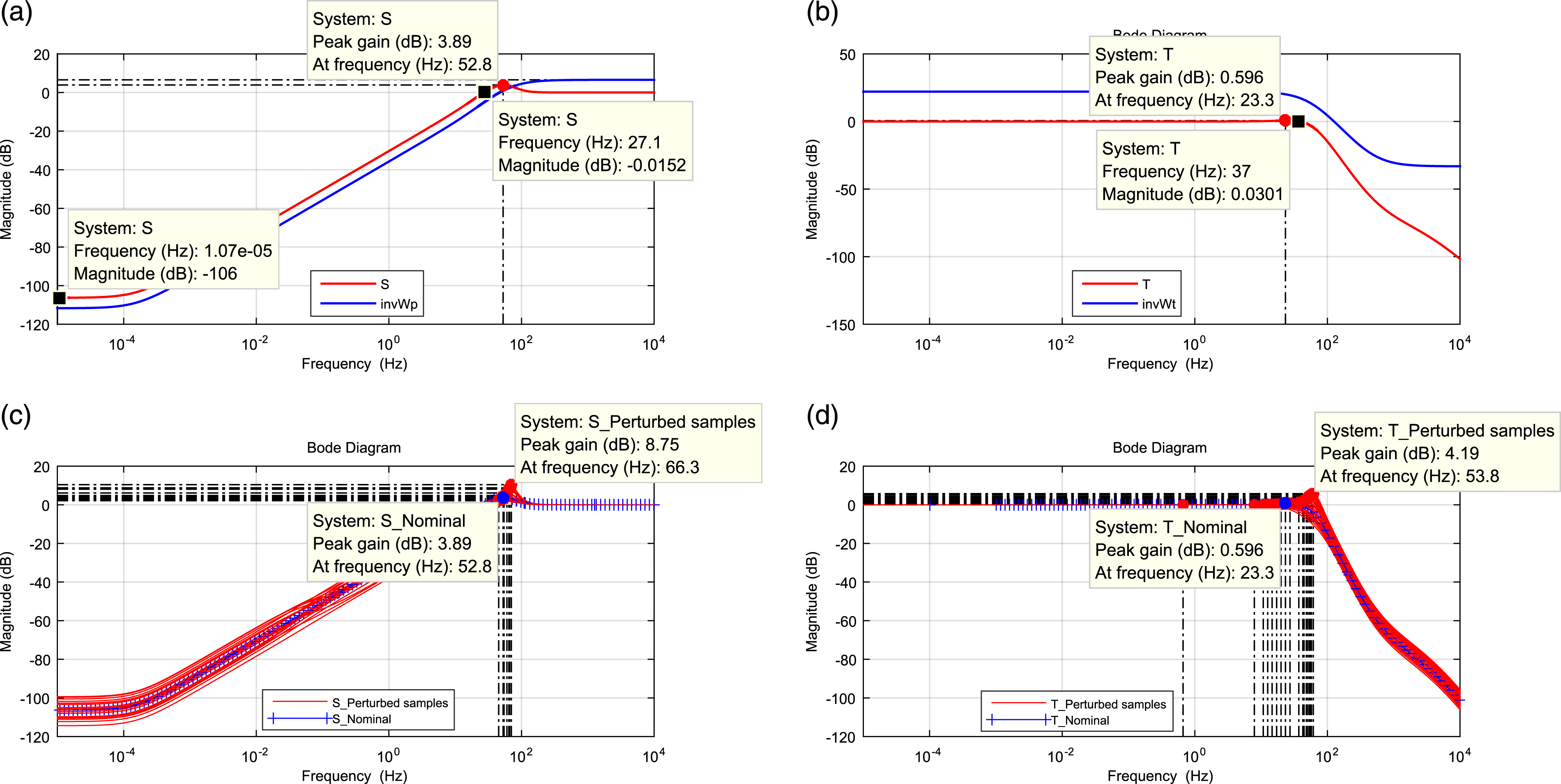$W_{P}^{- 1}$ and $S$ , (b) Bode magnitude plots of $W_{T}^{- 1}$ and $T$ , (c) Bode magnitude plot of the sensitivity function (S), and (d) Bode magnitude plot of the complementary sensitivity function (T).

Weight on the complementary sensitivity function, $W_{T}$ , is selected to satisfy maximum peak, $M_{T}$ is not more than 0.6, and attenuation of measurement noise, that is, $| T (jω) |$ is smaller when $ω \to \infty$ .

W_{T} = \frac{45.5 s^{3} + 49140 s^{2} + 1.769 e 7 s + 2.123 e 9}{s^{3} + 9000 s^{2} + 2.7 e 7 s + 2.7 e 10}

(30)

The sensitivity function must be small at low-frequency range to attenuate disturbance effects and also for set-point tracking. Hence, $W_{p}$ weight must have high gain at lower frequencies, that is, it should be a low-pass filter. Similarly, the complimentary sensitivity function must be small at high-frequency range to attenuate high-frequency noise and plant uncertainty at high-frequency range (Fang et al., 2015a, 2015b).

The two AREs are solved to get the $H_{\infty}$ controller by minimizing the cost function gamma $(γ)$ as explained in Section 4. The $H_{\infty}$ controller obtained is of eighth order.

The gain corresponding to the maximum singular value of the closed-loop system is a measure of optimality in the $H_{\infty}$ control theory. The $H_{\infty}$ norm of the closed-loop system is found to be 1.864 (i.e., $γ$ = 1.864), which is an optimal solution for the given plant with the designed controller.

Figure 11(c) shows that peak value of the nominal sensitivity function is 3.89 dB and worst-case peak value is 8.75 dB. Figure 11(d) shows that peak value of the nominal complementary sensitivity function is 0.596 dB and worst-case peak value is 4.19 dB.

The resultant eighth-order controller is as given in equation (31). The reduced third-order controller is obtained using the algorithm BALMR in Matlab Robust Control Tool Box shown in equation (32). It was observed that further model reduction did not retain the required performance

\frac{915.4 s^{7} + 1.917 e 8 s^{6} + 1.752 e 12 s^{5} + 5.671 e 15 s^{4} + 7.076 e 18 s^{3} + 2.258 e 21 s^{2} + 2.042 e 23 s + 6.451 e 22}{s^{8} + 2.25 e 5 s^{7} + 5.041 e 9 s^{6} + 9.049 e 12 s^{5} + 7.163 e 15 s^{4} + 3.03 e 18 s^{3} + 5.881 e 20 s^{2} + 3.905 e 22 s + 3.905 e 19}

(31)

\frac{252.3 s^{2} + 1.011 e 06 s + 3.471 e 05}{s^{3} + 654.1 s^{2} + 2.1 e 05 s + 210.2}

(32)

The frequency response characteristics of eighth-, third-, and second-order controllers are compared in Figure 12(a).

Figure 12.

Bode plots of the controller and compensated system in open loop and closed loop. (a) Bode plot of eighth order and reduced third- and second-order controllers, (b) compensated system stability margins with third-order controller, (c) closed-loop response of perturbed systems, and (d) closed-loop response of the nominal system.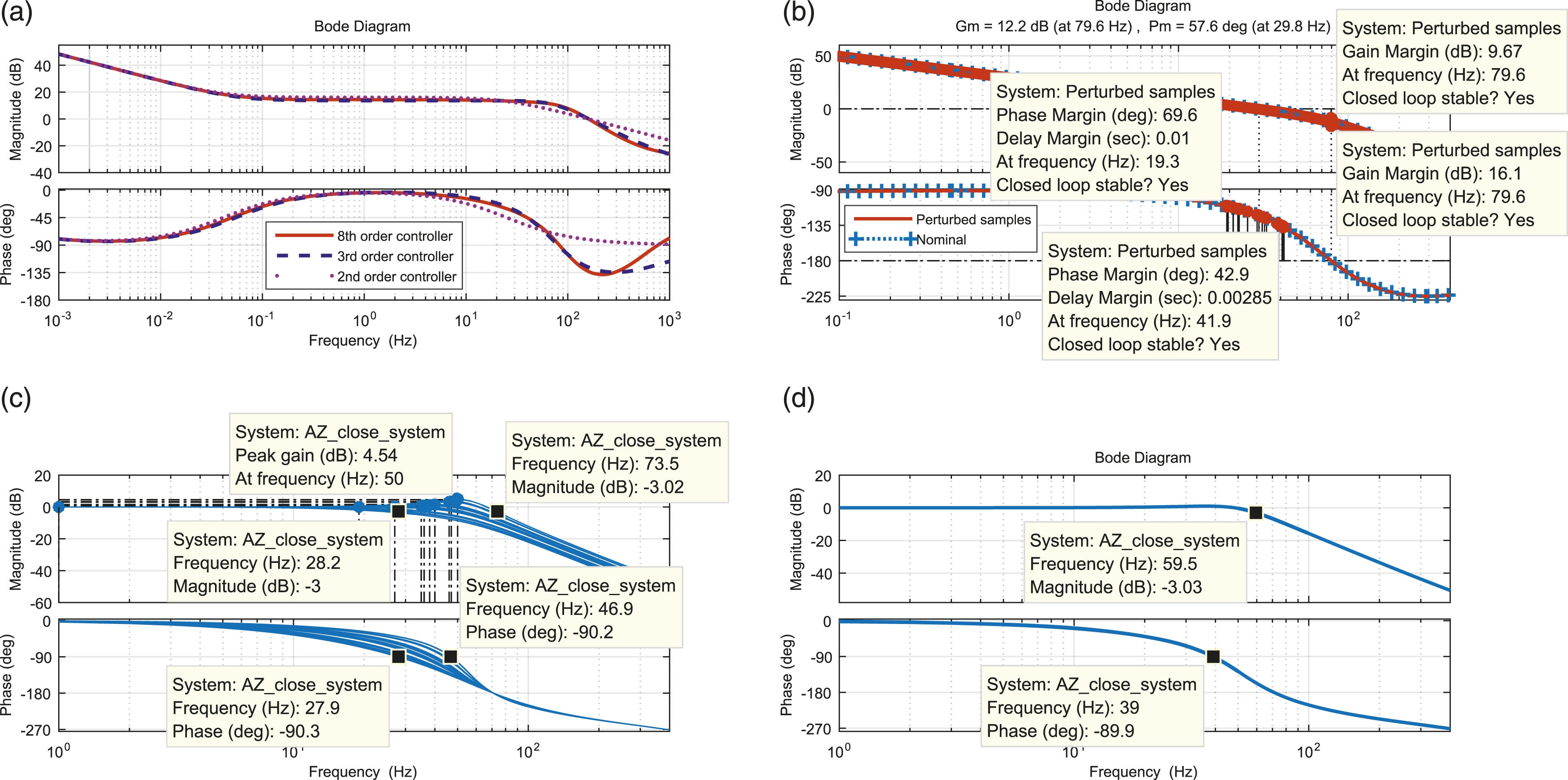

Figure 12(b) shows the stability margins of the nominal and the worst-case system. The gain margin is varying from 9.67 to 16.1 dB and the phase margin is 42.9–69.6 deg., whereas the nominal compensated system has a gain margin of 12.2 dB and phase margin of 57.6 deg.

Figure 12(c) shows that the bandwidth (at -90 deg. phase) of the closed-loop system varies from 27.9 to 46.9 Hz as the parameters of the plant vary and the worst-case peak of the closed-loop system is 4.54 dB (1.68).

Figure 12(d) shows the bandwidth of the nominal closed-loop system of 39 Hz. From this simulation/analysis, the designed controller is satisfying the design specifications mentioned in Section 1.

6. Controller implementation in digital signal processor

This third-order compensator was realized in digital domain using the digital signal processor (DSP) (TMS320F2812). The analog compensator was digitized using the Tustin method. Sampling was done at 3 kHz. The digital compensator (in the $z$ domain) is given in equation (33)

\frac{0.06455 - 0.01223 z^{- 1} + 0.06454 z^{- 2} + 0.01224 z^{- 3}}{1 - 2.779 z^{- 1} + 2.58 z^{- 2} + 0.801 z^{- 3}}

(33)

Simulation and practical results achieved with this compensator are tabulated in Table 2. Figure 13 shows the achieved experimental closed-loop system response, and Figure 14 shows transient response characteristics when the system is subjected to a body disturbance of 16 deg/s at 1 Hz. It can be seen that all the design parameters are met.

Table 2.

Achieved parameters of the compensated system.

Description	Design specifications	Simulation results	Achieved results
Gain margin	≥9 dB	12.2 dB	11.5 dB
Phase margin	≥40 deg	57.6 deg	55 deg
Closed-loop bandwidth	≥25 Hz	39 Hz	29.6 Hz
Damping coefficient	0.5–0.7	0.58	0.56

Figure 13.

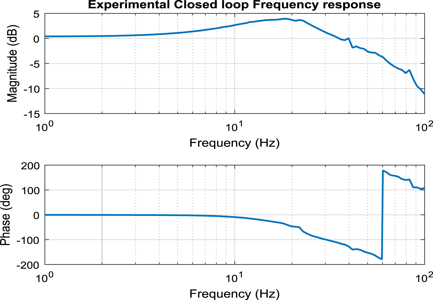
Closed-loop system response.

Figure 14.

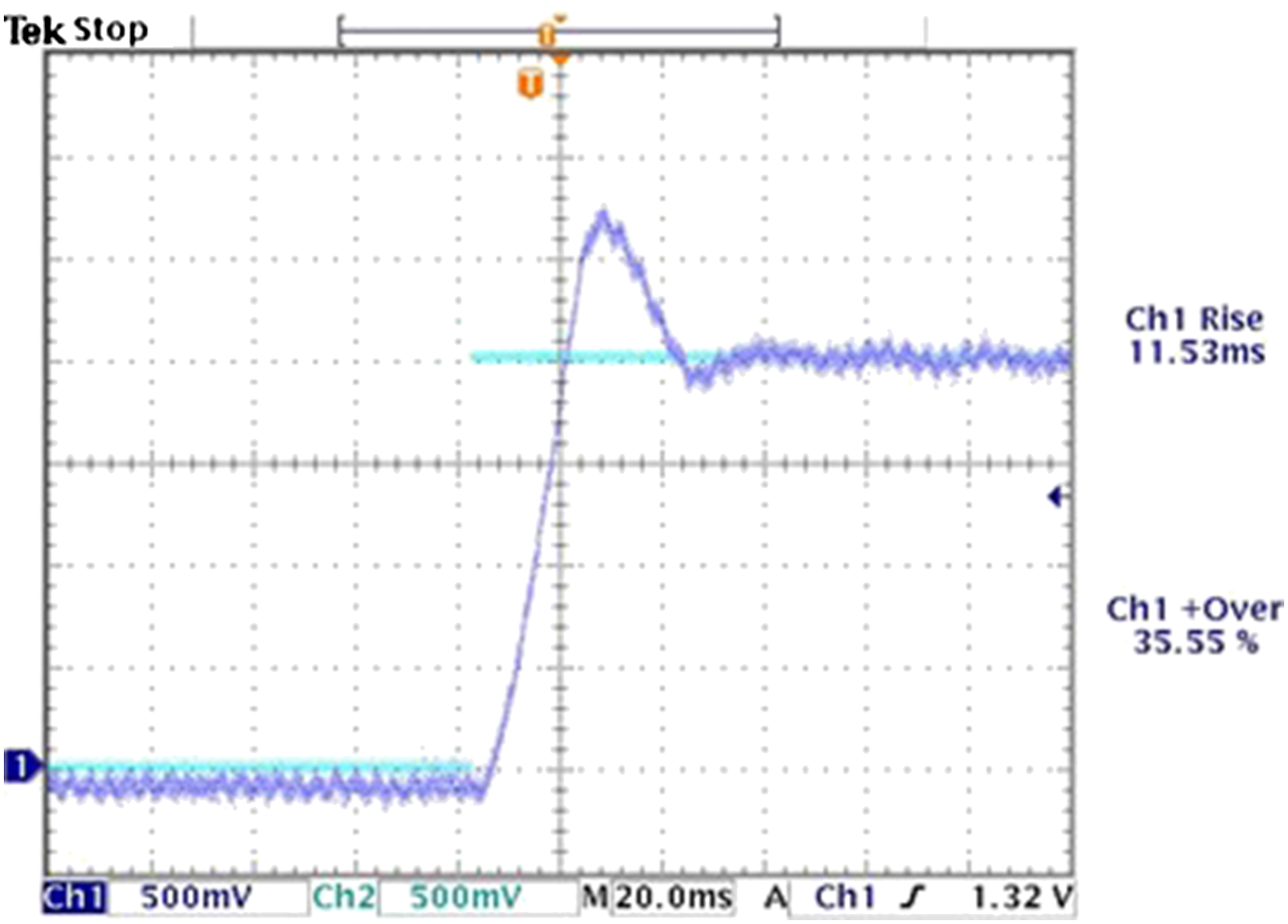
Step response of the system.

7. Conclusion

This study presents modeling of the two-axis gimbal system using an experimental approach and a mathematical formulation of the system. The $H_{\infty}$ controller is designed by using the mixed sensitivity approach. The rate of LOS is stabilized in the azimuth axis with a high degree of disturbance. The designed controller is implemented in DSP-based hardware, and the specifications for the robust stability and command following are met.

Footnotes

Declaration of conflicting interests

The authors declared no potential conflicts of interest with respect to the research, authorship, and/or publication of this article.

Funding

The authors received no financial support for the research, authorship, and/or publication of this article.

ORCID iD

M. Ashok Kumar

References

Abdo

Vali

Toloei

, et al. (2014) Stabilization loop of a two axes gimbal system using self-tuning PID type fuzzy controller. ISA Transactions 53(2): 591–602.

Ashok Kumar

Kanthalakshmi

(2018) H_∞ tracking control for an inverted pendulum. Journal of Vibration and Control 24(16): 3515–3524.

Balas

Chiang

Packard

, et al. (2008) Robust Control Toolbox-User’s Guide. Natick, MA: The MathWorks Inc.

Davidson

Ushakumari

(2016) H-infinity loop shaping controller for load frequency control of a deregulated power system. Procedia Technology 25: 775–784.

Fang

Yin

Lei

(2015a) An adaptive decoupling control for three-axis gyro stabilized platform based on neural networks. Mechatronics 27: 38–46.

Fang

Fei

Wang

(2015b) H-infinity control of MEMS gyroscope using TS fuzzy model. IFAC-PapersOnLine 48(14): 241–246.

Gawronski

(2007) Control and pointing challenges of large antennas and telescopes. IEEE Transactions on Control Systems Technology 15(2): 276–289.

Petkov

Konstantinov

(2005) Robust Control with MATLAB. London: Springer-Verlag.

Hong

Cho

Park

, et al. (2011) Trajectory generation and H_∞ robust control for inertially stabilized system. In: IEEE/ASME international conference on advanced intelligent mechatronics, Budapest, Hungary, 3–7 July 2011, pp. 695–700. IEEE.

10.

Kwakernaak

(1993) Robust control and H-Infinity optimization-tutorial paper. Automatica 29(2): 255–273.

11.

Mackenroth

(2010) Robust Control Systems, Theory and Case Studies. New Delhi: Springer India Pvt. Ltd.

12.

McFarlane

Glover

(1992) A loop-shaping design procedure using H/sub infinity/synthesis. IEEE Transactions on Automatic Control 37(6): 759–769.

13.

Skogestad

Postlethwaite

(2007) Multivariable Feedback Control: Analysis and Design. New York: Wiley.

14.

Toloei

Pirzadeh

Vali

(2016) Design of predictive control and evaluate the effects of flight dynamics on performance of one axis gimbal system, considering disturbance torques. Aerospace Science and Technology 54: 143–150.

15.

Wang

Yao

Wang

Guan

(2014) Line-of-sight stabilization system based on fractional-order control. Advanced Materials Research 962–965: 2703–2707.

H ∞ Control law for line of sight stabilization in two-axis gimbal system

Abstract

Keywords

1. Introduction

2. Model of two-axis gimbal system

3. Perturbation model

4. H ∞ Control methodology

4.1. Mixed sensitivity design

5. H ∞ Controller design

6. Controller implementation in digital signal processor

7. Conclusion

Footnotes

Declaration of conflicting interests

Funding

ORCID iD

References

4. $H_{\infty}$ Control methodology

5. $H_{\infty}$ Controller design