A numerical approach for solving fractional optimal control problems with mittag-leffler kernel

Abstract

In this work, we present a numerical approach based on the shifted Legendre polynomials for solving a class of fractional optimal control problems. The derivative is described in the Atangana–Baleanu derivative sense. To solve the problem, operational matrices of AB-fractional integration and multiplication, together with the Lagrange multiplier method for the constrained extremum, are considered. The method reduces the main problem to a system of nonlinear algebraic equations. In this framework by solving the obtained system, the approximate solution is calculated. An error estimate of the numerical solution is also proved for the approximate solution obtained by the proposed method. Finally, some illustrative examples are presented to demonstrate the accuracy and validity of the proposed scheme.

Keywords

Fractional optimal control problems atangana–baleanu derivative shifted legendre polynomials operational matrix lagrange multiplier method

1. Introduction

Since approximately the year 2000, fractional calculus theory has gained substantial popularity and significance. It has tremendously attractive applications in diverse and widespread fields of physics and engineering, such as rheology, viscoelasticity, electromagnetic theory, diffusive transport, fluid flow, and electrical networks (Ali et al., 2020; Aydogan et al., 2020; Kilbas et al., 2006; Mainardi, 2010; Podlubny, 1999; Samko et al., 1993; Zaslavsky, 2005). Fractional order models are often more accurate than classical integer order descriptions because fractional order derivatives and integrals embed the description of the memory and hereditary properties of different substances (Baleanu and Mendes Lopes, 2019). These derivatives are useful in rheology as crucial features of cell rheological behavior (Djordjevic et al., 2003). Recently, many authors have modeled the dynamics of novel coronavirus (2019-nCov) with fractional derivative (see Ahmed et al., 2020; Hussain et al., 2020; Khan and Atangana, 2020).

The most important fractional operators (FOs) are the Riemann–Liouville (RL) and Caputo. Because a kernel of type local and singular exists in the definition of these operators, it is difficult or impossible to describe many nonlocal dynamic systems. Hence, many authors have introduced several definitions for fractional integral and derivative operators with the nonlocal and non-singular kernel such as Caputo–Fabrizio (CF) (Caputo and Fabrizio, 2015); Losada and Nieto, 2015) and Atangana–Baleanu (Atangana and Baleanu, 2016).

The optimal control theory is an area in mathematics which has been under development for years. The FOCPs as a development of the classical optimal control problems (OCPs) are getting more and more popular. In these problems, the dynamical system and (or) the objective function may be involved with FOs. For more details, see Bahaa (2017) and references therein.

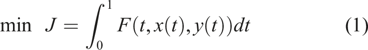
An FOCP can be defined with respect to different definitions of FOs. In this work, we numerically investigate the FOCPs in which FO is defined in the AB derivative sense as follows

\min J = \int_{0}^{1} F (t, x (t), y (t)) d t

(1)

Subject to fractional dynamic system

{}^{A B C}{D_{t}^{ω}} x (t) = ξ (t) x (t) + η (t) y (t)

(2)

And the initial condition

x (0) = b

(3)

where 0 < ω ≤ 1, F is given continuous function, ξ and η are given known functions, and y, x, and J are called the control, the state functions, and the performance index, respectively. In Lotfi et al. (2011), the above problems (1)–(3), is discussed with the Caputo fractional derivative. In Dehestani and Ordokhani (2020), Heydari (2020), Sweilam et al. (2020), Tajadodi et al. (2021), authors have considered different models of FOCPs and have presented various methods for solving these types of problems.

Orthogonal basis functions have been generally used to achieve approximate solution for many problems in various fields of science. Approximation of the solution using these functions is known as a useful tool in solving many classes of equations numerically, for example, differential equations (Ganji et al., 2020a; Jafari et al., 2019; Sadeghi et al., 2020), partial differential equations (Tajadodi, 2020; Tuan et al., 2020b), integro-differential equations (Ganji et al., 2020b; Jafari et al., 2021; Tuan et al., 2020a), and FOCPs (Heydari et al., 2020; Lotfi et al., 2011; Nemati, 2016) of various orders (fixed, fractional, or variable order).

The order of this article is as follows: In Section 2, we recall basic definitions of fractional operators. The main properties of the SLPs are presented in Section 3. Section 4 is devoted to proposing a numerical method for solving problems (1)–(3), while an error estimate of the numerical solution is discussed in Section 5. Section 6 includes some illustrative examples. Finally, we conclude the article in Section 7.

2. Basic definitions

The main aim of this section is to recall those definitions of the FOs which will be used further.

Definition 1

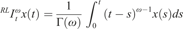
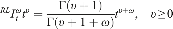
(See Podlubny, 1999 ) Let 0 < ω ≤ 1. The RL integral is defined as

{}^{R L}{I_{t}^{ω}} x (t) = \frac{1}{Γ (ω)} \int_{0}^{t} {(t - s)}^{ω - 1} x (s) d s

The RL integral of order ω satisfies the following property

{}^{R L}{I_{t}^{ω}} t^{υ} = \frac{Γ (υ + 1)}{Γ (υ + 1 + ω)} t^{υ + ω}, υ \geq 0

Definition 2

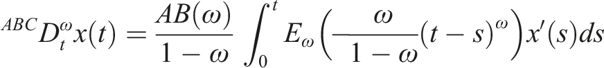
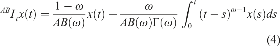
(See Atangana and Baleanu, 2016). Let 0 < ω ≤ 1, x ∈ H¹(0, 1) and AB(ω) be a normalization function such that AB(0) = AB(1) = 1 and $A B (ω) = 1 - ω + ω / Γ (ω)$ . Then

1. The AB derivative is defined as

{}^{A B C}{D_{t}^{ω}} x (t) = \frac{A B (ω)}{1 - ω} \int_{0}^{t} E_{ω} (- \frac{ω}{1 - ω} {(t - s)}^{ω}) x^{'} (s) d s

where

E_{ω} (t) = \sum_{i = 0}^{\infty} t^{i} / Γ (ω i + 1)

is the Mittag-Leffler function.

2. The AB integral is given as

{}^{A B}I {}_{t}^{ω}x (t) = \frac{1 - ω}{A B (ω)} x (t) + \frac{ω}{A B (ω) Γ (ω)} \int_{0}^{t} {(t - s)}^{ω - 1} x (s) d s

(4)

Let

α_{ω} = 1 - ω / A B (ω)

and

β_{ω} = 1 / A B (ω) Γ (ω)

; then, we can rewrite (4) as

{}^{A B}{I_{t}^{ω}} x (t) = α_{ω} x (t) + β_{ω} Γ (ω + 1) {}^{R L}{I_{t}^{ω}} x (t)

It is easy to report that the AB integral satisfies the following properties (Abdeljawad and Baleanu, 2016; Abdeljawad, 2017; Abdeljawad and Baleanu, 2017):

1. ${}^{A B}{I_{t}^{ω}} C = C (α_{ω} + β_{ω} t^{ω}), C \in ℝ$ ,

2. ${}^{A B}{I_{t}^{ω}} t^{υ} = t^{υ} (α_{ω} + β_{ω} (υ + ω + 1) B (υ + 1, ω + 1) t^{ω})$ , where B(⋅, ⋅) is the Beta function, and

3. ${}^{A B}{I_{t}^{ω}} ({}^{A B C}{D_{t}^{ω}} x (t)) = x (t) - x (0)$ .

Theorem 1

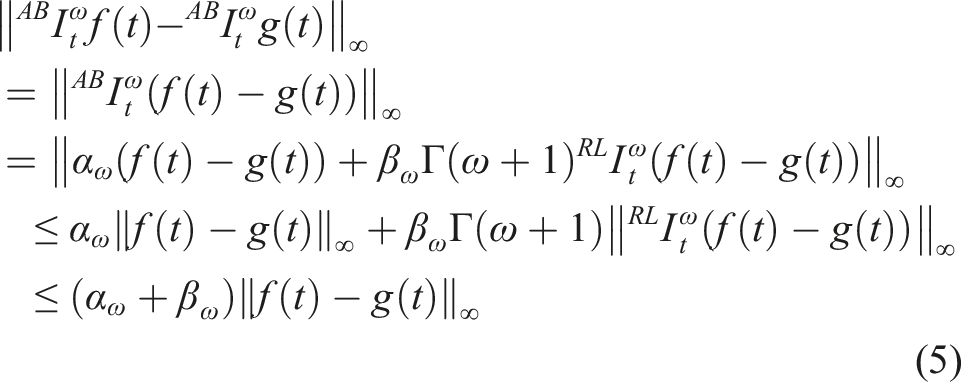
Let C[0, 1] be the space of all continuous functions defined on [0, 1] and f, g ∈ C[0, 1]. Then, the following inequality can be established

{‖ {}^{A B}{I_{t}^{ω}} f (t) - {}^{A B}{I_{t}^{ω}} g (t) ‖}_{\infty} \leq ε {‖ f (t) - g (t) ‖}_{\infty}

where ɛ = α_ω + β_ω.

Proof

According to definition of the AB integral, we have

\begin{array}{l} {‖ {}^{A B}{I_{t}^{ω}} f (t) -^{A B} I_{t}^{ω} g (t) ‖}_{\infty} = {‖ {}^{A B}{I_{t}^{ω}} (f (t) - g (t)) ‖}_{\infty} \\ = {‖ α_{ω} (f (t) - g (t)) + β_{ω} Γ (ω + 1) {}^{R L}{I_{t}^{ω}} (f (t) - g (t)) ‖}_{\infty} \\ \leq α_{ω} {‖ f (t) - g (t) ‖}_{\infty} + β_{ω} Γ (ω + 1) {‖ {}^{R L}{I_{t}^{ω}} (f (t) - g (t)) ‖}_{\infty} \\ \leq (α_{ω} + β_{ω}) {‖ f (t) - g (t) ‖}_{\infty} \end{array}

(5)

Taking ɛ = α_ω + β_ω, the proof is complete.

Theorem 2

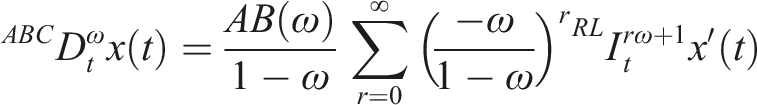
(See Tajadodi, 2020 ). Let 0 < ω ≤ 1. Then, we can rewrite the AB derivative by

{}^{A B C}{D_{t}^{ω}} x (t) = \frac{A B (ω)}{1 - ω} \sum_{r = 0}^{\infty} {(\frac{- ω}{1 - ω})}^{r} {}^{R L}{I_{t}^{r ω + 1}} x^{'} (t)

3. The SLPs and operational matrices based on the SLPs

In this section, we present some of the main properties of the SLPs.

3.1. The SLPs

The explanation of the SLPs on [0, 1] is

ℒ_{n} (t) = L_{n} (2 t - 1), n = 0, 1, 2, \dots,

where L_n(t) is the well-known Legendre polynomial (LP) of degree n. The recursive formula of LP on [−1, 1] given by

\begin{array}{l} L_{0} (t) = 1 \\ L_{1} (t) = t \\ L_{n + 1} (t) = \frac{2 n + 1}{n + 1} t L_{n} (t) - \frac{n}{n + 1} L_{n - 1} (t), n = 1, 2, 3, \dots \end{array}

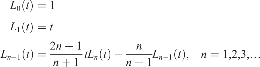
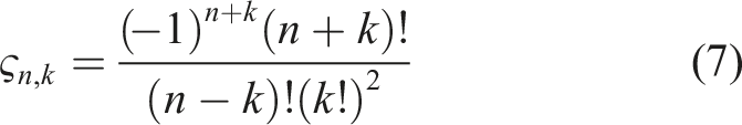
The analytic form of the SLPs of degree n is defined by

ℒ_{n} (t) = \sum_{k = 0}^{n} ς_{n, k} t^{k}

(6)

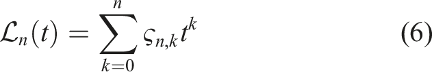
Where

ς_{n, k} = \frac{{(- 1)}^{n + k} (n + k)!}{(n - k)! {(k!)}^{2}}

(7)

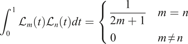
The orthogonality property is satisfied for the SLPs as follows

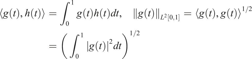
\int_{0}^{1} ℒ_{m} (t) ℒ_{n} (t) d t = {\begin{array}{l} \frac{1}{2 m + 1} & m = n \\ 0 & m \neq n \end{array}

For two arbitrary functions g, h ∈ L²[0, 1], the inner product and norm in this space are defined, respectively, by

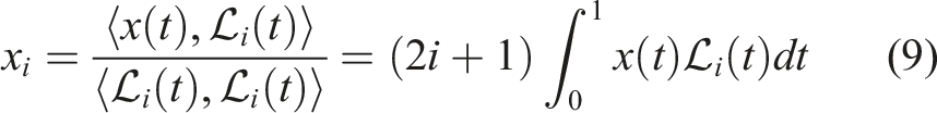
〈 g (t), h (t) 〉 = \int_{0}^{1} g (t) h (t) d t, {‖ g (t) ‖}_{L^{2} [0,1]} = {〈 g (t), g (t) 〉}^{1 / 2} = {(\int_{0}^{1} {| g (t) |}^{2} d t)}^{1 / 2}

Suppose that x(t) ∈ L²[0, 1]. Then, the function x(t) can be expanded in terms of the SLPs by

x (t) = \sum_{i = 0}^{\infty} x_{i} ℒ_{i} (t)

(8)

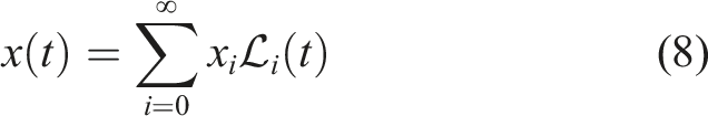
where

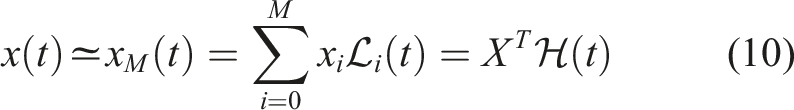
x_{i} = \frac{〈 x (t), ℒ_{i} (t) 〉}{〈 ℒ_{i} (t), ℒ_{i} (t) 〉} = (2 i + 1) \int_{0}^{1} x (t) ℒ_{i} (t) d t

(9)

By taking only the first M + 1 terms in (8), x(t) can be approximated as

x (t) ≃ x_{M} (t) = \sum_{i = 0}^{M} x_{i} ℒ_{i} (t) = X^{T} ℋ (t)

(10)

where

X = {[x_{0}, x_{1}, \dots, x_{M}]}^{T}

and

ℋ (t) = {[ℒ_{0} (t), ℒ_{1} (t), \dots, ℒ_{M} (t)]}^{T}

(11)

Theorem 3

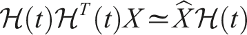
(See Ganji et al, 2020b ). The OM of the product of the vector $ℋ (t)$ given by (11) can be approximated as

ℋ (t) ℋ^{T} (t) X ≃ \hat{X} ℋ (t)

where $\hat{X}$ is given in Ganji et al. (2020b).

Theorem 4

Suppose 0 < ω ≤ 1 and $ℋ (t)$ be the SLPs vector defined by (11), then

{}^{A B}{I_{t}^{ω}} ℋ (t) ≃ ℐ^{ω} ℋ (t)

where

ℐ^{ω} = α_{ω} I + β_{ω} Γ (ω + 1) Ω^{ω}

is called the OM of the AB integral based on the SLPs and I is an (M + 1) × (M + 1) identity matrix. Also, Ω^ω is called the OM of RL integral based on the SLPs which is given by

Ω^{ω} = [\begin{matrix} σ_{0,0,0} & σ_{0,1,0} & \dots & σ_{0, M, 0} \\ \sum_{l = 0}^{1} σ_{1,0, l} & \sum_{s = 0}^{1} σ_{1,1, l} & \dots & \sum_{s = 0}^{1} σ_{1, M, l} \\ ⋮ & ⋮ & \dots & ⋮ \\ \sum_{l = 0}^{M} σ_{M, 0, l} & \sum_{l = 0}^{M} σ_{M, 1, l} & \dots & \sum_{l = 0}^{M} σ_{M, M, l} \end{matrix}]

With

σ_{i, s, l} = \frac{Γ (s + 1) ς_{i, l} d_{l, s}}{Γ (l + ω + 1)}

Proof

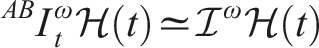
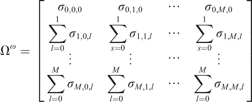
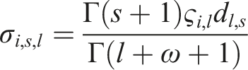
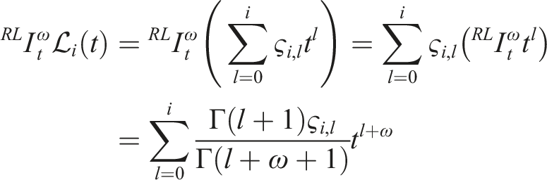
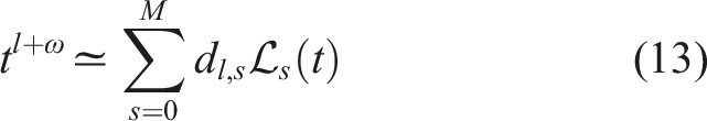
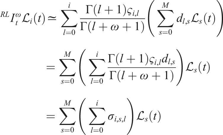
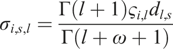
By applying the AB integral operator, ${}^{A B}{I_{t}^{ω}}$ , on $ℋ (t)$ yields

{}^{A B}{I_{t}^{ω}} ℋ (t) = α_{ω} ℋ (t) + β_{ω} Γ (ω + 1) {}^{R L}{I_{t}^{ω}} ℋ (t)

(12)

Now, we must obtain the OM of RL integral of order ω. To do this, we apply the LR integral operator, ${}^{R L}{I_{t}^{ω}}$ , on $ℒ_{i} (t), i = 0, 1, \dots, M$ as

{}^{R L}{I_{t}^{ω}} ℒ_{i} (t) = {}^{R L}{I_{t}^{ω}} (\sum_{l = 0}^{i} ς_{i, l} t^{l}) = \sum_{l = 0}^{i} ς_{i, l} ({}^{R L}{I_{t}^{ω}} t^{l}) = \sum_{l = 0}^{i} \frac{Γ (l + 1) ς_{i, l}}{Γ (l + ω + 1)} t^{l + ω}

By approximating the function t^l+ω in terms of the SLPs, we have

t^{l + ω} ≃ \sum_{s = 0}^{M} d_{l, s} ℒ_{s} (t)

(13)

In view of (13) and for i = 0, 1, …, M, we get

\begin{array}{l} {}^{R L}{I_{t}^{ω}} ℒ_{i} (t) ≃ \sum_{l = 0}^{i} \frac{Γ (l + 1) ς_{i, l}}{Γ (l + ω + 1)} (\sum_{s = 0}^{M} d_{l, s} ℒ_{s} (t)) \\ = \sum_{s = 0}^{M} (\sum_{l = 0}^{i} \frac{Γ (l + 1) ς_{i, l} d_{l, s}}{Γ (l + ω + 1)}) ℒ_{s} (t) \\ = \sum_{s = 0}^{M} (\sum_{l = 0}^{i} σ_{i, s, l}) ℒ_{s} (t) \end{array}

Therefore, for i = 0, 1, …, M, we can write

{}^{R L}{I_{t}^{ω}} ℋ (t) = Ω^{ω} ℋ (t)

(14)

Where

Ω^{ω} = [\begin{matrix} σ_{0,0,0} & σ_{0,1,0} & \dots & σ_{0, M, 0} \\ \sum_{l = 0}^{1} σ_{1,0, l} & \sum_{l = 0}^{1} σ_{1,1, l} & \dots & \sum_{l = 0}^{1} σ_{1, M, l} \\ ⋮ & ⋮ & \dots & ⋮ \\ \sum_{l = 0}^{M} σ_{M, 0, l} & \sum_{l = 0}^{M} ρ_{M, 1, l} & \dots & \sum_{l = 0}^{M} σ_{M, M, l} \end{matrix}]

With

σ_{i, s, l} = \frac{Γ (l + 1) ς_{i, l} d_{l, s}}{Γ (l + ω + 1)}

By substituting (14) into (12), the proof completes.

4. Numerical method

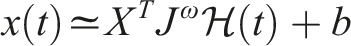
Here, we present a numerical method for solving the FOCP (1)–(3). For this purpose, first we approximate ${}^{A B C}{D_{t}^{ω}} x (t)$ as

{}^{A B C}{D_{t}^{ω}} x (t) ≃ X^{T} ℋ (t)

(15)

where

X = {[\begin{matrix} x_{0}, x_{1}, \dots, c_{M} \end{matrix}]}^{T}

By taking the AB integral of (15) and using the initial condition, we have

x (t) ≃ X^{T} J^{ω} ℋ (t) + b

By approximating

b ≃ X_{0}^{T} ℋ (t)

, x(t) could be rewritten as

x (t) ≃ γ ℋ (t)

(16)

where

γ = X^{T} J^{ω} + X_{0}^{T}

, and the elements of vector X₀ can be computed by (9).

We expand the variable t and the function y(t) in terms of the SLPs as

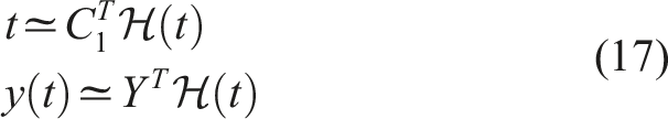
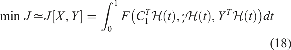
\begin{array}{l} t ≃ C_{1}^{T} ℋ (t) \\ y (t) ≃ Y^{T} ℋ (t) \end{array}

(17)

By substituting (16) and (17) into the performance index, we obtain

\min J ≃ J [X, Y] = \int_{0}^{1} F (C_{1}^{T} ℋ (t), γ ℋ (t), Y^{T} ℋ (t)) d t

(18)

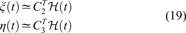
Now, we approximate the functions ξ(t) and η(t) as

\begin{array}{l} ξ (t) ≃ C_{2}^{T} ℋ (t) \\ η (t) ≃ C_{3}^{T} ℋ (t) \end{array}

(19)

According to the product operational matrix of the shifted Legendre basis and using (16), (17), and (19), we can write

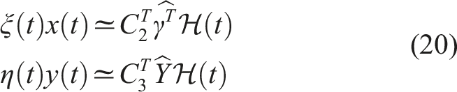
\begin{array}{l} ξ (t) x (t) ≃ C_{2}^{T} \hat{γ^{T}} ℋ (t) \\ η (t) y (t) ≃ C_{3}^{T} \hat{Y} ℋ (t) \end{array}

(20)

Then, using (15) and (20), the dynamic system given by (2) is converted to

X^{T} - C_{2}^{T} \hat{γ^{T}} - C_{3}^{T} \hat{Y} = 0

(21)

Moreover, according to the Lagrange multiplier for minimizing (18) subject to the condition given in (21), we define

J^{*} [X, Y, λ] = J [X, Y] + (X^{T} - C_{2}^{T} \hat{γ^{T}} - C_{3}^{T} \hat{Y}) λ

(22)

where

λ = {[\begin{matrix} λ_{0}, λ_{1}, \dots, λ_{M} \end{matrix}]}^{T}

is the unknown Lagrange multiplier. Now, the necessary optimality conditions are as follows

\frac{\partial J^{*}}{\partial X} = 0, \frac{\partial J^{*}}{\partial Y} = 0, \frac{\partial J^{*}}{\partial λ} = 0

(23)

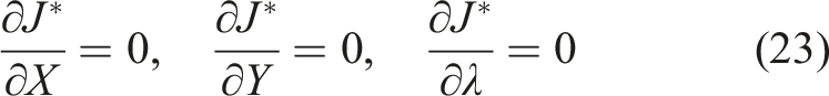
In view of (23), we have a system of nonlinear algebraic equations. The unknown parameters of the vectors X, Y, and λ are computed by solving this system. Finally, approximations of the optimal control and corresponding state functions are given by (16) and (17), respectively.

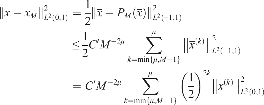
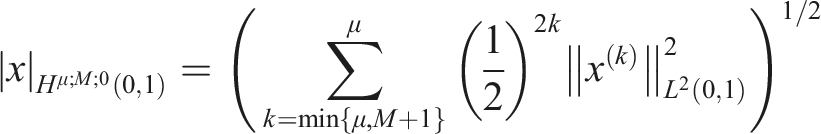
5. Error bound

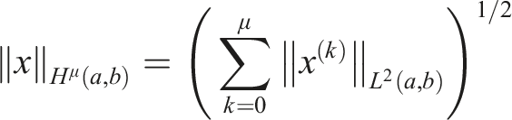
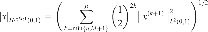
The Sobolev norm of integer order μ ≥ 0 in the interval (a, b) is given by

{‖ x ‖}_{H^{μ} (a, b)} = {(\sum_{k = 0}^{μ} {‖ x^{(k)} ‖}_{L^{2} (a, b)})}^{1 / 2}

where x^(k) denotes the kth derivative of x and H^μ(a, b) is a Sobolev space.

Lemma 1

(See Canuto et al,. 2006 ). Let μ ≥ 0 and x ∈ H^m(−1, 1). Suppose that $P_{M} (x) = \sum_{i = 0}^{M} x_{i} L_{i} (t)$ be the truncated Legendre series of x. Then,

{‖ x - P_{M} (x) ‖}_{L^{2} (- 1,1)} \leq C M^{- μ} {| x |}_{H^{μ; M} (- 1,1)}

where

{| x |}_{H^{μ; M} (- 1,1)} = {(\sum_{k = \min {μ, M + 1}}^{μ} {‖ x^{(k)} ‖}_{L^{2} (- 1,1)}^{2})}^{1 / 2}

and C is a positive constant independent of function x and integer M.

Lemma 2

(See Ganji et al., 2020b ). Let $x : (0, 1) \to ℝ$ be a function in H^μ(0, 1). Suppose that function $\bar{x} : (- 1, 1) \to ℝ$ is given by $\bar{x} (t) = x (1 / 2 (t + 1))$ for all t ∈ (−1, 1). Then, for 0 ≤ k ≤ μ

{‖ {\bar{x}}^{(k)} ‖}_{L^{2} (- 1,1)} = 2^{1 / 2 - k} {‖ x^{(k)} ‖}_{L^{2} (0,1)}

Theorem 5

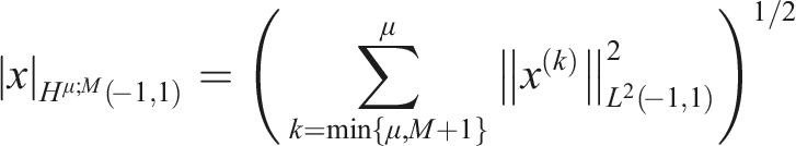
Suppose μ ≥ 0 and x ∈ H^μ(0, 1). Let $x_{M} (t) = \sum_{i = 0}^{M} x_{i} ℒ_{i} (t)$ is the approximate solution obtained by the proposed method in Section 4. Then,

{‖ x - x_{M} ‖}_{L^{2} (0,1)} \leq C M^{- μ} {| x |}_{H^{μ; M; 0} (0,1)}

And

{‖ x^{'} - x_{M}^{'} ‖}_{L^{2} (0,1)} \leq C^{*} M^{- μ} {| x |}_{H^{μ; M; 1} (0,1)}

Where

{| x |}_{H^{μ; M; r} (0,1)} = {(\sum_{k = \min {μ, M + 1}}^{μ} {(\frac{1}{2})}^{2 k} {‖ x^{(k + r)} ‖}_{L^{2} (0,1)}^{2})}^{1 / 2}, r = 0, 1

Proof

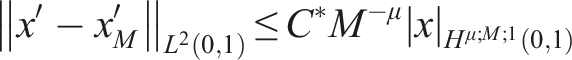
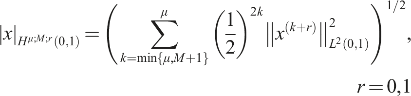
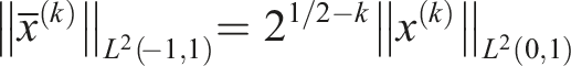
With the help of Lemma 2, we obtain

\begin{array}{l} {‖ x - x_{M} ‖}_{L^{2} (0,1)}^{2} = \frac{1}{2} {‖ \bar{x} - P_{M} (\bar{x}) ‖}_{L^{2} (- 1,1)}^{2} \\ \leq \frac{1}{2} C^{'} M^{- 2 μ} \sum_{k = \min {μ, M + 1}}^{μ} {‖ {\bar{x}}^{(k)} ‖}_{L^{2} (- 1,1)}^{2} \\ = C^{'} M^{- 2 μ} \sum_{k = \min {μ, M + 1}}^{μ} {(\frac{1}{2})}^{2 k} {‖ x^{(k)} ‖}_{L^{2} (0,1)}^{2} \end{array}

By definition

{| x |}_{H^{μ; M; 0} (0,1)} = {(\sum_{k = \min {μ, M + 1}}^{μ} {(\frac{1}{2})}^{2 k} {‖ x^{(k)} ‖}_{L^{2} (0,1)}^{2})}^{1 / 2}

The proof is complete. In a similar way, we obtain

{‖ x^{'} - x_{M}^{'} ‖}_{L^{2} (0,1)} \leq C^{*} M^{- μ} {| x |}_{H^{μ; M; 1} (0,1)}

where

{| x |}_{H^{μ; M; 1} (0,1)} = {(\sum_{k = \min {μ, M + 1}}^{μ} {(\frac{1}{2})}^{2 k} {‖ x^{(k + 1)} ‖}_{L^{2} (0,1)}^{2})}^{1 / 2}

Theorem 6

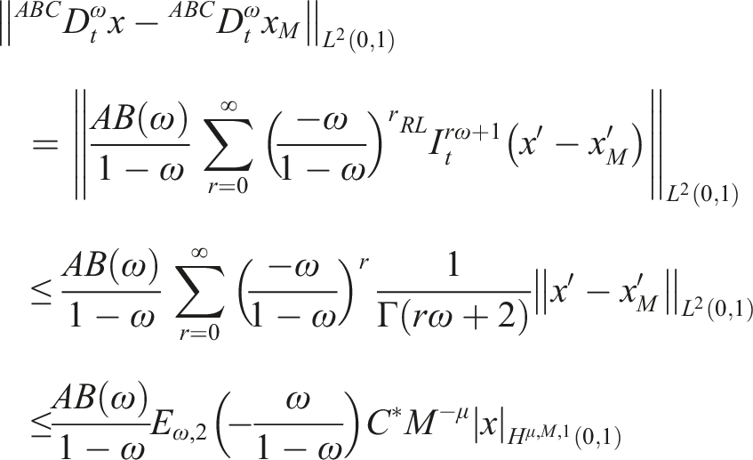
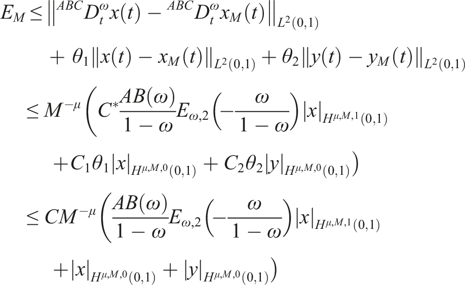
Suppose that 0 < ω ≤ 1 and x ∈ H^μ(0, 1) satisfies in Theorem 5. Then

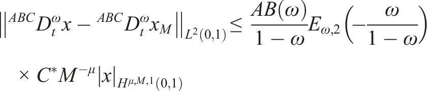
\begin{array}{l} {‖ {}^{A B C}{D_{t}^{ω}} x - {}^{A B C}{D_{t}^{ω}} x_{M} ‖}_{L^{2} (0,1)} \leq \frac{A B (ω)}{1 - ω} E_{ω, 2} (- \frac{ω}{1 - ω}) \\ \times C^{*} M^{- μ} {| x |}_{H^{μ, M, 1} (0,1)} \end{array}

Proof

By using Theorems 2 and 5, we get

\begin{array}{l} {‖ {}^{A B C}{D_{t}^{ω}} x - {}^{A B C}{D_{t}^{ω}} x_{M} ‖}_{L^{2} (0,1)} \\ = {‖ \frac{A B (ω)}{1 - ω} \sum_{r = 0}^{\infty} {(\frac{- ω}{1 - ω})}^{r} {}^{R L}{I_{t}^{r ω + 1}} (x^{'} - x_{M}^{'}) ‖}_{L^{2} (0,1)} \\ \leq \frac{A B (ω)}{1 - ω} \sum_{r = 0}^{\infty} {(\frac{- ω}{1 - ω})}^{r} \frac{1}{Γ (r ω + 2)} {‖ x^{'} - x_{M}^{'} ‖}_{L^{2} (0,1)} \\ \leq \frac{A B (ω)}{1 - ω} E_{ω, 2} (- \frac{ω}{1 - ω}) C^{*} M^{- μ} {| x |}_{H^{μ, M, 1} (0,1)} \end{array}

Theorem 7

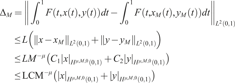
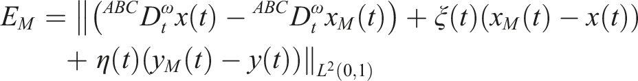
Suppose that μ ≥ 0 and x, y ∈ H^μ(0, 1) satisfy in Theorems 5 and 6. Let F satisfies the Lipschitz conditions with the constant L and $θ_{1} = \max_{0 \leq t \leq 1} | ξ (t) |, θ_{2} = \max_{0 \leq t \leq 1} | η (t) |$ . Then, $Δ_{M} = {‖ J - J_{M} ‖}_{L^{2} (0,1)}$ and E_M, the error bound of the proposed method, are bounded as follows

\begin{array}{l} Δ_{M} \leq LC M^{- μ} ({| x |}_{H^{μ, M, 0} (0,1)} + {| y |}_{H^{μ, M, 0} (0,1)}) \\ E_{M} \leq C M^{- μ} (\frac{A B (ω)}{1 - ω} E_{ω, 2} (- \frac{ω}{1 - ω}) {| x |}_{H^{μ, M, 1} (0,1)} \\ + {| x |}_{H^{μ, M, 0} (0,1)} + {| y |}_{H^{μ, M, 0} (0,1)}) \end{array}

Proof

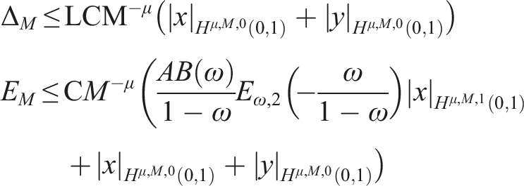
According to (1), we have

\begin{array}{l} Δ_{M} = {‖ \int_{0}^{1} F (t, x (t), y (t)) d t - \int_{0}^{1} F (t, x_{M} (t), y_{M} (t)) d t ‖}_{L^{2} (0,1)} \\ \leq L ({‖ x - x_{M} ‖}_{L^{2} (0,1)} + {‖ y - y_{M} ‖}_{L^{2} (0,1)}) \\ \leq L M^{- μ} (C_{1} {| x |}_{H^{μ, M, 0} (0,1)} + C_{2} {| y |}_{H^{μ, M, 0} (0,1)}) \\ \leq LC M^{- μ} ({| x |}_{H^{μ, M, 0} (0,1)} + {| y |}_{H^{μ, M, 0} (0,1)}) \end{array}

where C = max{C₁, C₂}. Also, in view of (2), we can write

\begin{array}{l} E_{M} = ‖ ({}^{A B C}{D_{t}^{ω}} x (t) - {}^{A B C}{D_{t}^{ω}} x_{M} (t)) + ξ (t) (x_{M} (t) - x (t)) \\ {+ η (t) (y_{M} (t) - y (t)) ‖}_{L^{2} (0,1)} \end{array}

Because

θ_{1} = \max_{0 \leq t \leq 1} | ξ (t) |, θ_{2} = \max_{0 \leq t \leq 1} | η (t) |

, we have

\begin{array}{l} E_{M} \leq {‖ {}^{A B C}{D_{t}^{ω}} x (t) - {}^{A B C}{D_{t}^{ω}} x_{M} (t) ‖}_{L^{2} (0,1)} \\ + θ_{1} {‖ x (t) - x_{M} (t) ‖}_{L^{2} (0,1)} + θ_{2} {‖ y (t) - y_{M} (t) ‖}_{L^{2} (0,1)} \\ \leq M^{- μ} (C^{*} \frac{A B (ω)}{1 - ω} E_{ω, 2} (- \frac{ω}{1 - ω}) {| x |}_{H^{μ, M, 1} (0,1)} \\ + C_{1} θ_{1} {| x |}_{H^{μ, M, 0} (0,1)} + C_{2} θ_{2} {| y |}_{H^{μ, M, 0} (0,1)}) \\ \leq C M^{- μ} (\frac{A B (ω)}{1 - ω} E_{ω, 2} (- \frac{ω}{1 - ω}) {| x |}_{H^{μ, M, 1} (0,1)} \\ + {| x |}_{H^{μ, M, 0} (0,1)} + {| y |}_{H^{μ, M, 0} (0,1)}) \end{array}

where

C = \max {C^{*}, C_{1} θ_{1}, C_{2} θ_{2}}

6. Test examples

This section includes some illustrative examples which show the accuracy and efficiency of the proposed method.

Example 1

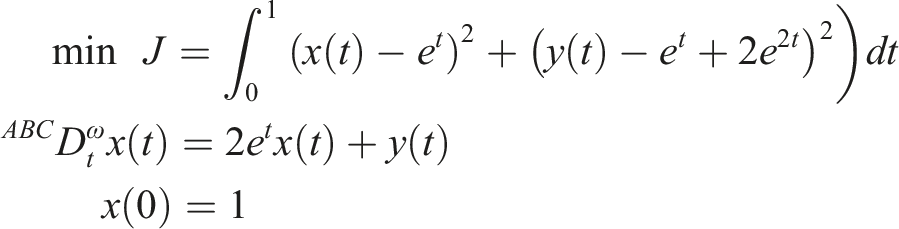
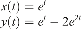
Consider the following FOCP

\begin{array}{l} \min J = \int_{0}^{1} {(x (t) - e^{t})}^{2} + {(y (t) - e^{t} + 2 e^{2 t})}^{2}) d t \\ {}^{A B C}{D_{t}^{ω}} x (t) = 2 e^{t} x (t) + y (t) \\ x (0) = 1 \end{array}

where

\begin{array}{l} x (t) = e^{t} \\ y (t) = e^{t} - 2 e^{2 t} \end{array}

when ω = 1. We have applied the proposed method to this problem and reported the numerical results in Figures 1–3 and Tables 1 and 2 . By considering M = 5, the numerical solutions obtained by different values of ω together with the exact solution are displayed in Figure 1. Figure 2 shows the results obtained by different values of M and ω = 0.9. Comparison of L_∞-norm and L₂-norm errors is shown in Figure 3 and Table 1 . Table 2 reports the values of performance index by setting M = 5. From Figure 1 and Table 1 , we see that the numerical solution converges to the exact one when the value of ω tends to 1.

Figure 1.

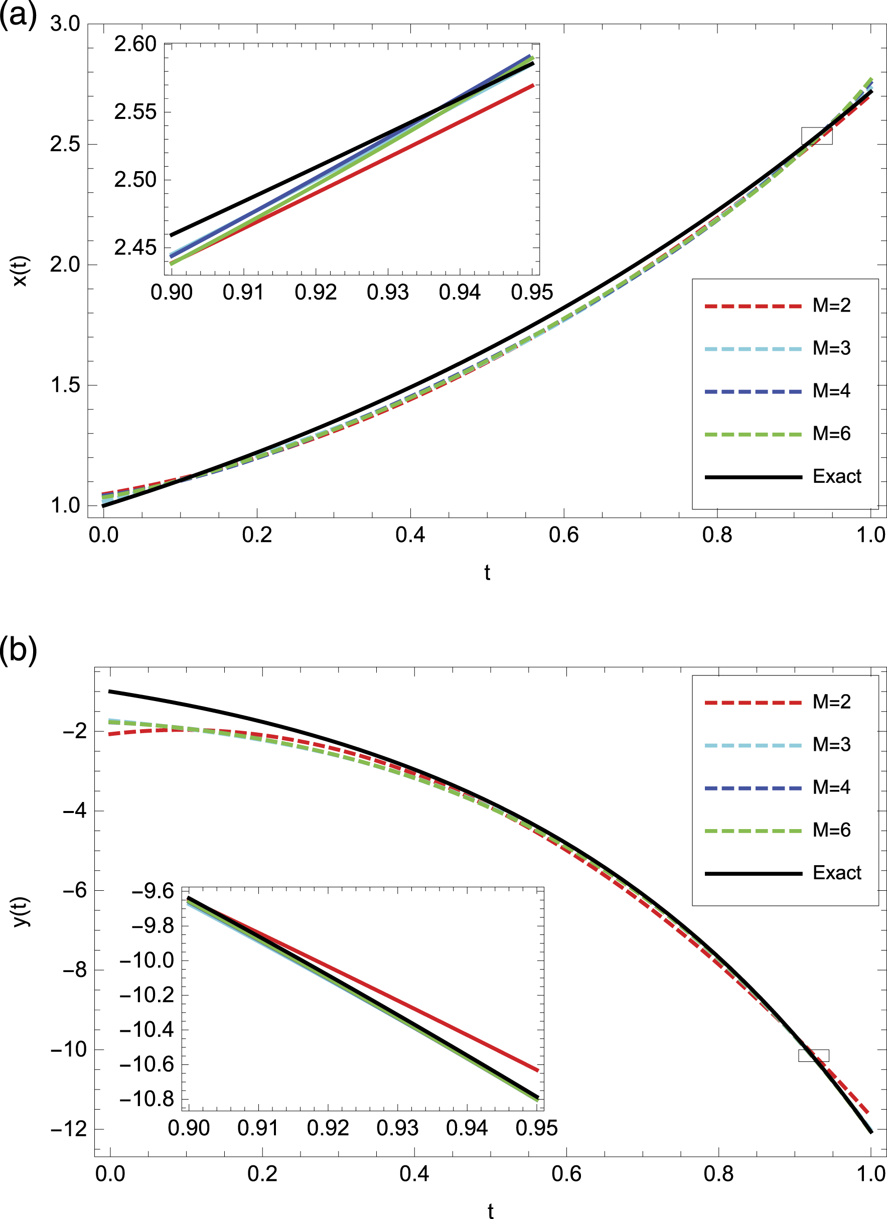
(Example 1) (a) The exact and approximate solutions (x(t)) and (b) the exact and approximate solutions (y(t)) and M = 5.

Figure 2.

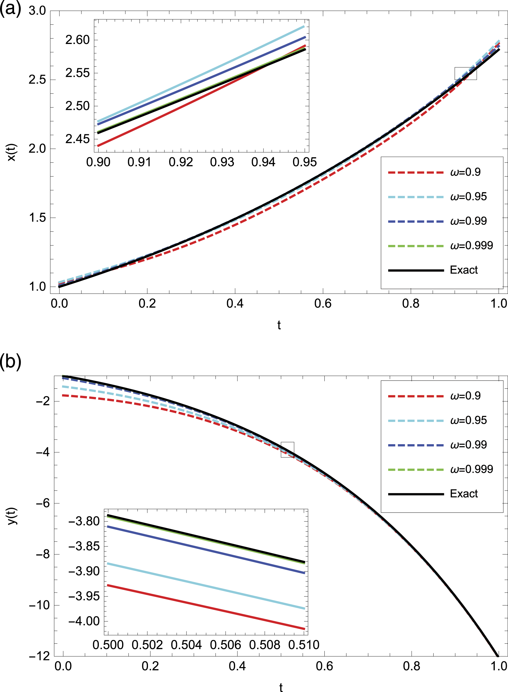
(Example 1) (a) The exact and approximate solutions (x(t)) and (b) the exact and approximate solutions (y(t)) and ω = 0.9.

Figure 3.

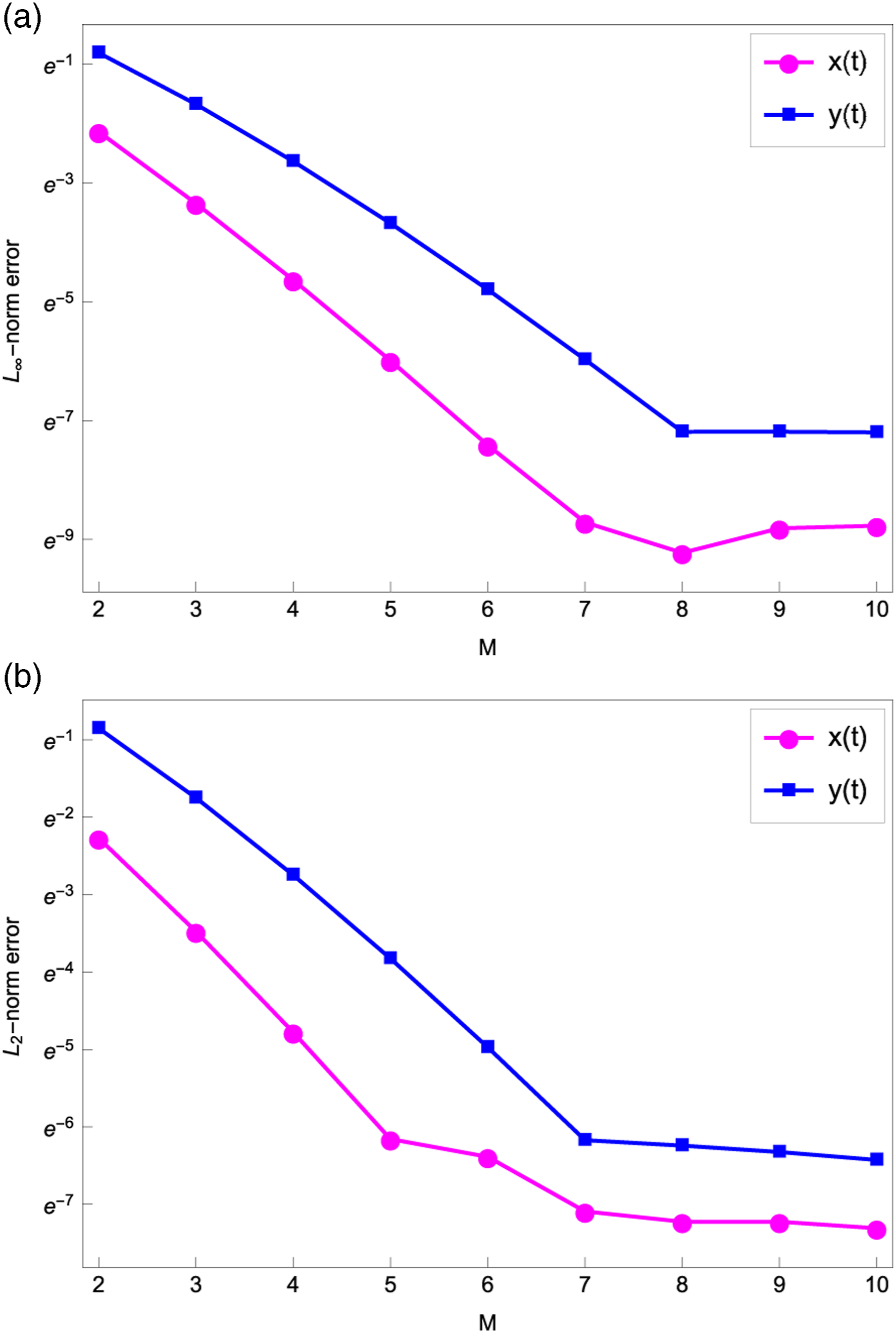
(Example 1) Comparison of (a) L_∞-norm error and (b) L₂-norm error by different values of M and ω = 1.

Table 1.

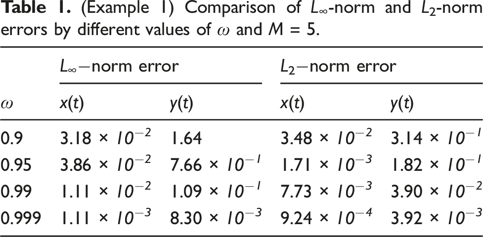
(Example 1) Comparison of L_∞-norm and L₂-norm errors by different values of ω and M = 5.

ω	L_∞−norm error		L₂−norm error
ω	x(t)	y(t)	x(t)	y(t)
0.9	3.18 × 10⁻²	1.64	3.48 × 10⁻²	3.14 × 10⁻¹
0.95	3.86 × 10⁻²	7.66 × 10⁻¹	1.71 × 10⁻³	1.82 × 10⁻¹
0.99	1.11 × 10⁻²	1.09 × 10⁻¹	7.73 × 10⁻³	3.90 × 10⁻²
0.999	1.11 × 10⁻³	8.30 × 10⁻³	9.24 × 10⁻⁴	3.92 × 10⁻³

Table 2.

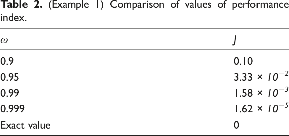
(Example 1) Comparison of values of performance index.

ω	J
0.9	0.10
0.95	3.33 × 10⁻²
0.99	1.58 × 10⁻³
0.999	1.62 × 10⁻⁵
Exact value	0

Example 2

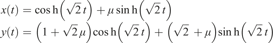
(See Lotfi et al., 2011 ; Nemati, 2016 ; Oh and Luus, 1989 ). Consider the following FOCP

\begin{array}{l} \min J = \int_{0}^{1} \frac{1}{2} (x {(t)}^{2} + y {(t)}^{2}) d t \\ {}^{A B C}{D_{t}^{ω}} x (t) = - x (t) + y (t) \\ x (0) = 1 \end{array}

With

\begin{array}{l} x (t) = cos h (\sqrt{2} t) + μ sin h (\sqrt{2} t) \\ y (t) = (1 + \sqrt{2} μ) cos h (\sqrt{2} t) + (\sqrt{2} + μ) sin h (\sqrt{2} t) \end{array}

when ω = 1 and

μ = - cos h (\sqrt{2}) + \sqrt{2} sin h (\sqrt{2}) / \sqrt{2} \cos (\sqrt{2} + sin h (\sqrt{2}))

. This problem is solved with different methods given in Lotfi et al. (2011), Nemati (2016) , Oh and Luus (1989) which include spectral method based on the second-kind Chebyshev polynomials, operational matrix, and orthogonal collocation method, respectively. Hence, in Tables 3 and 4 , the numerical results obtained via the proposed method are compared with the results given in Lotfi et al. (2011), Nemati (2016) , Oh and Luus (1989) at some selected points when ω = 1. Also, by considering M = 5, the numerical solutions obtained by different values of ω together with the exact solution are displayed in Figure 4, and comparison of L_∞-norm and L₂-norm errors is reported in Figure 5 and Table 5 .

Table 3.

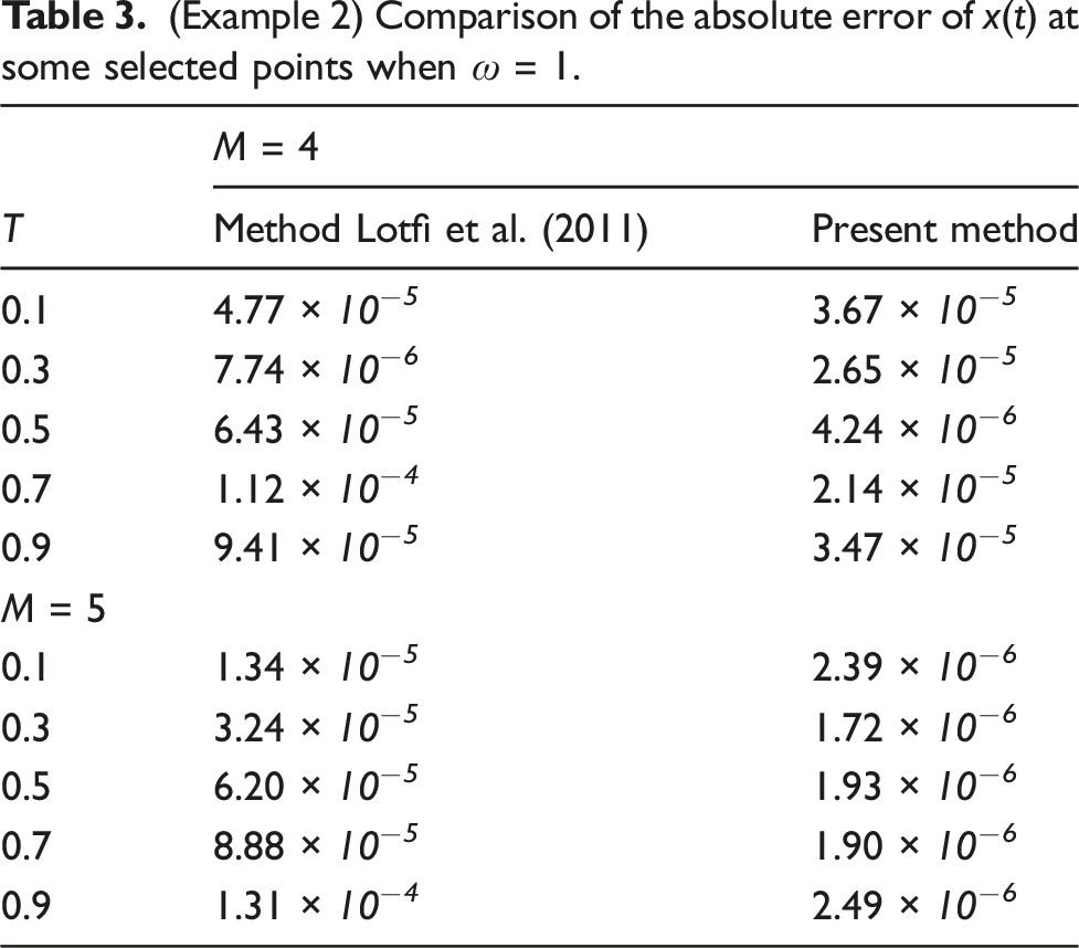
(Example 2) Comparison of the absolute error of x(t) at some selected points when ω = 1.

	M = 4
T	Method Lotfi et al. (2011)	Present method
0.1	4.77 × 10⁻⁵	3.67 × 10⁻⁵
0.3	7.74 × 10⁻⁶	2.65 × 10⁻⁵
0.5	6.43 × 10⁻⁵	4.24 × 10⁻⁶
0.7	1.12 × 10⁻⁴	2.14 × 10⁻⁵
0.9	9.41 × 10⁻⁵	3.47 × 10⁻⁵
M = 5
0.1	1.34 × 10⁻⁵	2.39 × 10⁻⁶
0.3	3.24 × 10⁻⁵	1.72 × 10⁻⁶
0.5	6.20 × 10⁻⁵	1.93 × 10⁻⁶
0.7	8.88 × 10⁻⁵	1.90 × 10⁻⁶
0.9	1.31 × 10⁻⁴	2.49 × 10⁻⁶

Table 4.

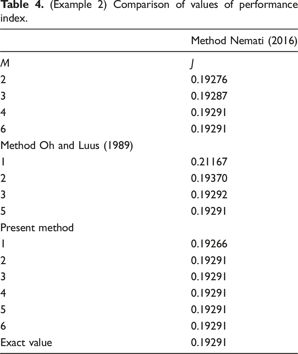
(Example 2) Comparison of values of performance index.

	Method Nemati (2016)
M	J
2	0.19276
3	0.19287
4	0.19291
6	0.19291
Method Oh and Luus (1989)
1	0.21167
2	0.19370
3	0.19292
5	0.19291
Present method
1	0.19266
2	0.19291
3	0.19291
4	0.19291
5	0.19291
6	0.19291
Exact value	0.19291

Figure 4.

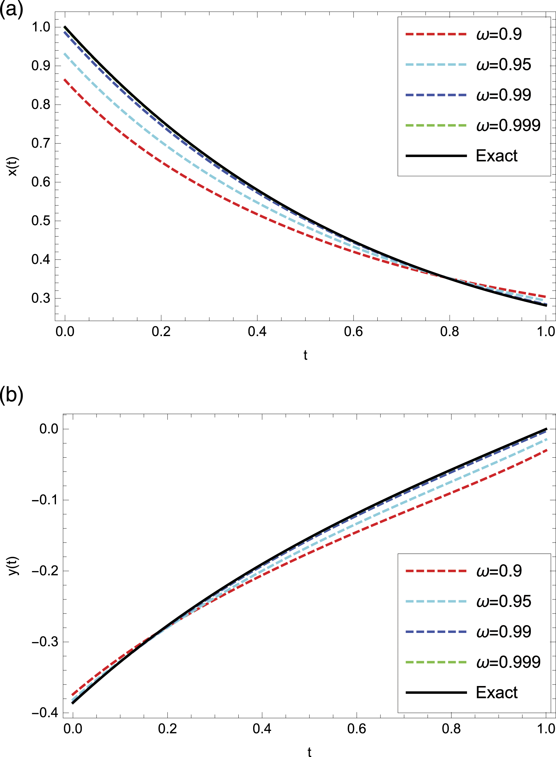
(Example 2) (a) The exact and approximate solutions (x(t)) and (b) the exact and approximate solutions (y(t)) and M = 5.

Figure 5.

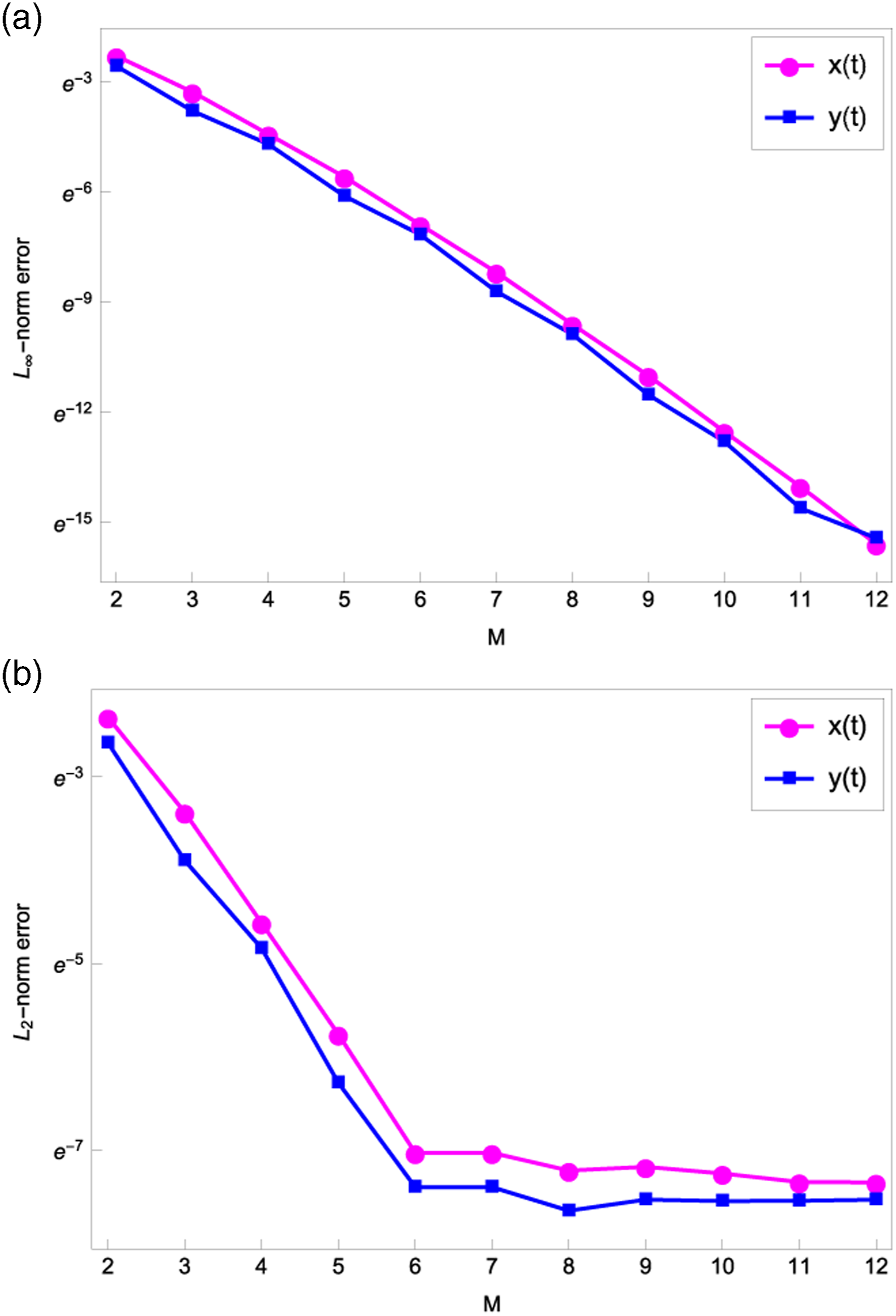
(Example 2) Comparison of (a) L_∞-norm error and (b) L₂-norm error by different values of M and ω = 1.

Table 5.

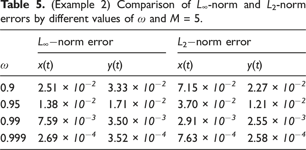
(Example 2) Comparison of L_∞-norm and L₂-norm errors by different values of ω and M = 5.

ω	L_∞−norm error		L₂−norm error
ω	x(t)	y(t)	x(t)	y(t)
0.9	2.51 × 10⁻²	3.33 × 10⁻²	7.15 × 10⁻²	2.27 × 10⁻²
0.95	1.38 × 10⁻²	1.71 × 10⁻²	3.70 × 10⁻²	1.21 × 10⁻²
0.99	7.59 × 10⁻³	3.50 × 10⁻³	2.91 × 10⁻³	2.55 × 10⁻³
0.999	2.69 × 10⁻⁴	3.52 × 10⁻⁴	7.63 × 10⁻⁴	2.58 × 10⁻⁴

Example 3

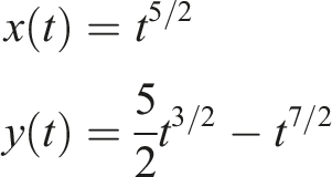
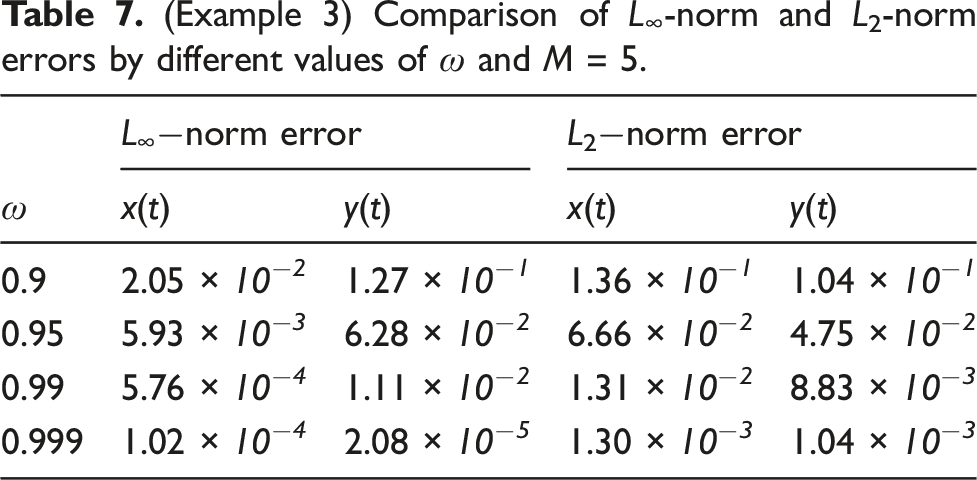
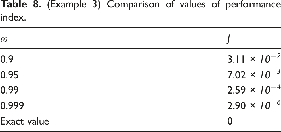
Consider the following FOCP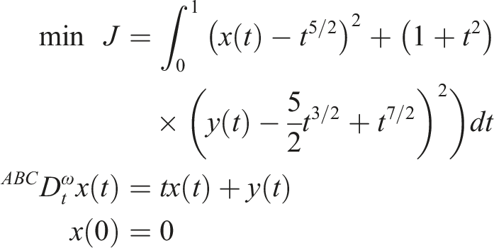

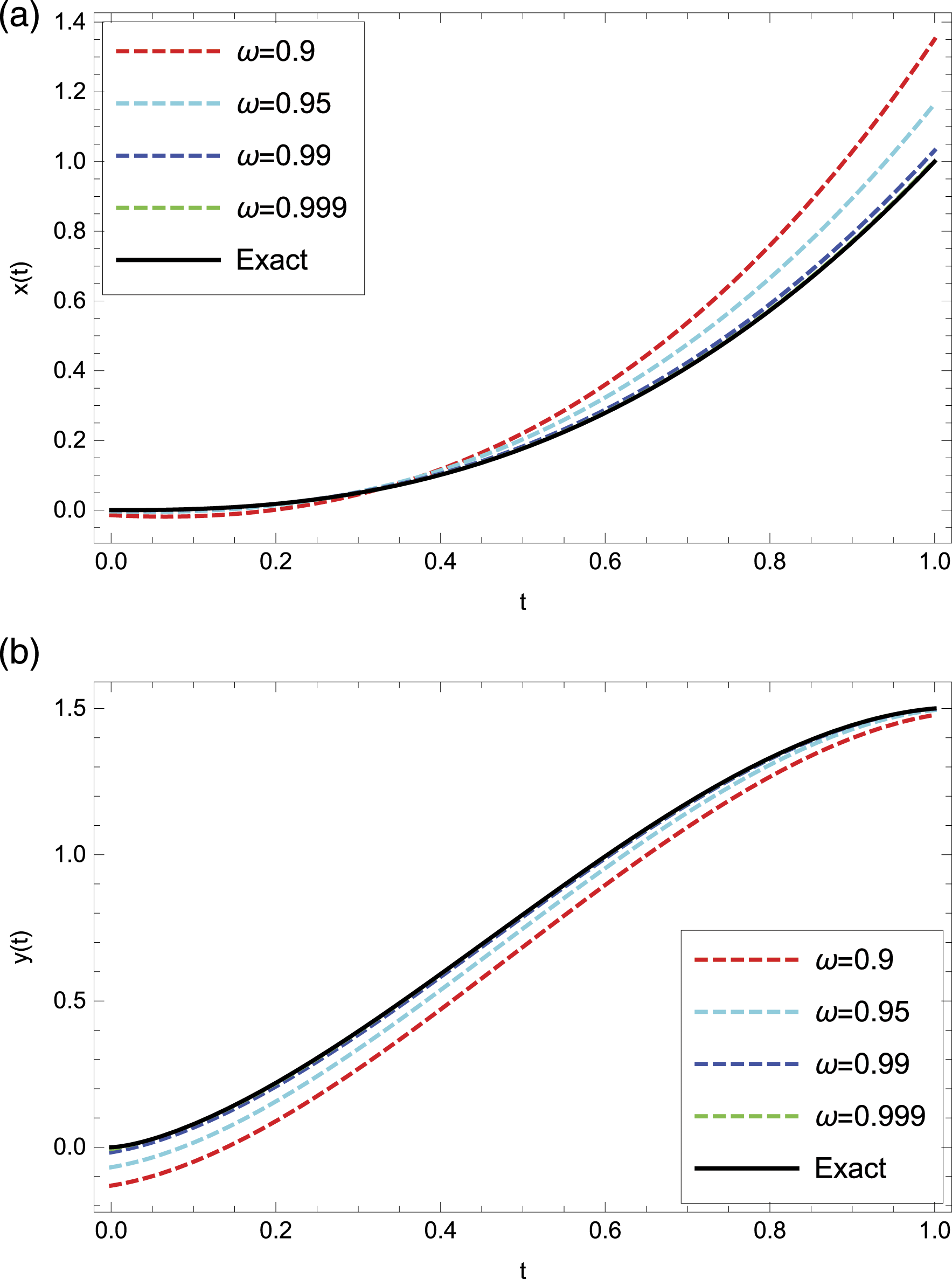
\begin{array}{l} \min J = \int_{0}^{1} {(x (t) - t^{5 / 2})}^{2} + (1 + t^{2}) {(y (t) - \frac{5}{2} t^{3 / 2} + t^{7 / 2})}^{2}) d t \\ {}^{A B C}{D_{t}^{ω}} x (t) = t x (t) + y (t) \\ x (0) = 0 \end{array}

where

\begin{array}{l} x (t) = t^{5 / 2} \\ y (t) = \frac{5}{2} t^{3 / 2} - t^{7 / 2} \end{array}

for ω = 1. By setting M = 5, the results obtained using the proposed method are shown by different values of ω in Figure 6 and Tables 6 – 8 . Also, comparison of L_∞-norm and L₂-norm errors for various values of M is plotted in Figure 7.

Figure 6.

(Example 3) (a) The exact and approximate solutions (x(t)) and (b) the exact and approximate solutions (y(t)) and M = 5.

Table 6.

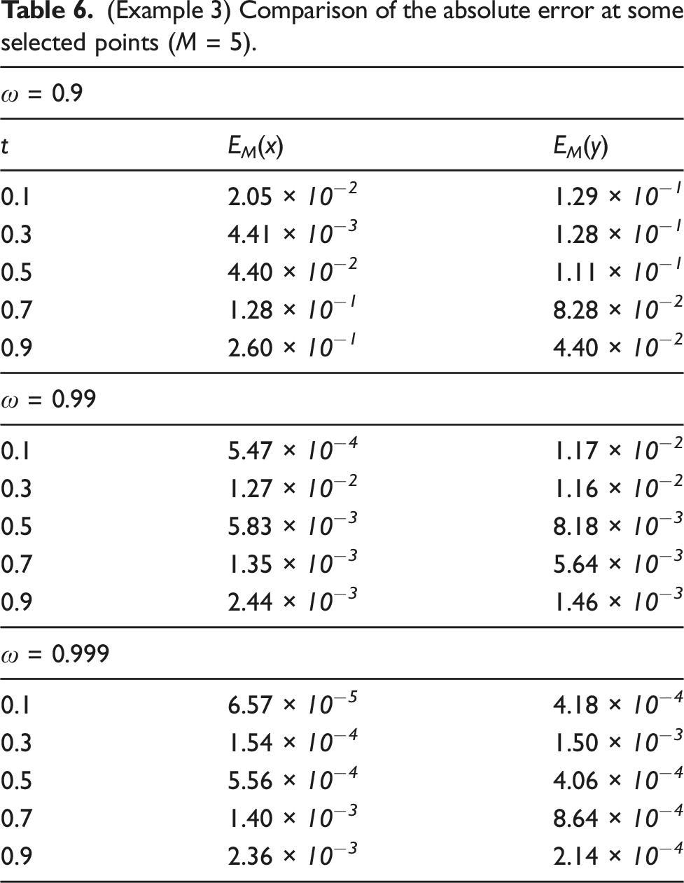
(Example 3) Comparison of the absolute error at some selected points (M = 5).

ω = 0.9
t	E_M(x)	E_M(y)
0.1	2.05 × 10⁻²	1.29 × 10⁻¹
0.3	4.41 × 10⁻³	1.28 × 10⁻¹
0.5	4.40 × 10⁻²	1.11 × 10⁻¹
0.7	1.28 × 10⁻¹	8.28 × 10⁻²
0.9	2.60 × 10⁻¹	4.40 × 10⁻²
ω = 0.99
0.1	5.47 × 10⁻⁴	1.17 × 10⁻²
0.3	1.27 × 10⁻²	1.16 × 10⁻²
0.5	5.83 × 10⁻³	8.18 × 10⁻³
0.7	1.35 × 10⁻³	5.64 × 10⁻³
0.9	2.44 × 10⁻³	1.46 × 10⁻³
ω = 0.999
0.1	6.57 × 10⁻⁵	4.18 × 10⁻⁴
0.3	1.54 × 10⁻⁴	1.50 × 10⁻³
0.5	5.56 × 10⁻⁴	4.06 × 10⁻⁴
0.7	1.40 × 10⁻³	8.64 × 10⁻⁴
0.9	2.36 × 10⁻³	2.14 × 10⁻⁴

Table 7.

(Example 3) Comparison of L_∞-norm and L₂-norm errors by different values of ω and M = 5.

ω	L_∞−norm error		L₂−norm error
ω	x(t)	y(t)	x(t)	y(t)
0.9	2.05 × 10⁻²	1.27 × 10⁻¹	1.36 × 10⁻¹	1.04 × 10⁻¹
0.95	5.93 × 10⁻³	6.28 × 10⁻²	6.66 × 10⁻²	4.75 × 10⁻²
0.99	5.76 × 10⁻⁴	1.11 × 10⁻²	1.31 × 10⁻²	8.83 × 10⁻³
0.999	1.02 × 10⁻⁴	2.08 × 10⁻⁵	1.30 × 10⁻³	1.04 × 10⁻³

Table 8.

(Example 3) Comparison of values of performance index.

ω	J
0.9	3.11 × 10⁻²
0.95	7.02 × 10⁻³
0.99	2.59 × 10⁻⁴
0.999	2.90 × 10⁻⁶
Exact value	0

Figure 7.

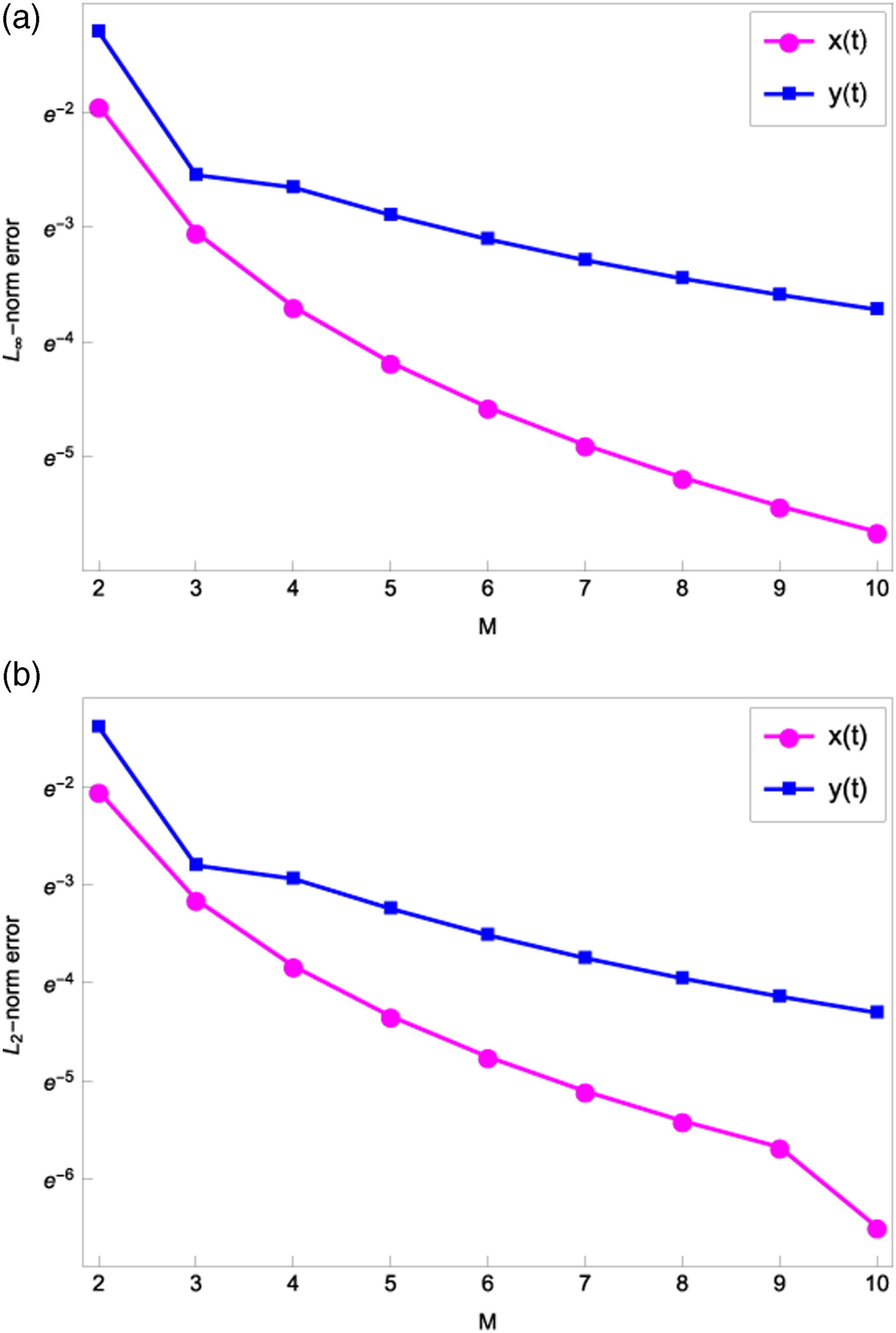
(Example 3) Comparison of (a) L_∞-norm error and (b) L₂-norm error by different values of M and ω = 1.

7. Conclusion

In this article, we have put forth a new numerical method for solving the fractional optimal control problems. By the definition of the Atangana–Baleanu integral operator and properties of the shifted Legendre polynomials (SLPs), the operational matrices of fractional integration and product have been presented. The approximation of the unknown function and its derivative in terms of the SLPs allow us to reduce the FOCPs to a set of nonlinear algebraic equations which greatly simplifies the problem. Then, an error analysis of this scheme has been given. Moreover, several examples have been presented to demonstrate the accuracy and efficiency of the proposed method. The numerical results show that the theoretical findings are in accordance with numerical experiments, and that the proposed algorithm is superior to others available in the literature. Finally, it seems that the global convergence and asymptotic stability of variable order FOCPs can be examined as further works for different type of fractional derivative.

Footnotes

Declaration of conflicting interests

The author(s) declared no potential conflicts of interest with respect to the research, authorship, and/or publication of this article.

Funding

The author(s) received no financial support for the research, authorship, and/or publication of this article.

ORCID iDs

Hossein Jafari

Dumitru Baleanu

References

Abdeljawad

Baleanu

(2016) Discrete fractional differences with nonsingular discrete mittag-leffler kernels. Advances in Difference Equations 232: 18.

Abdeljawad

(2017) A lyapunov type inequality for fractional operators with nonsingular mittag-leffler kernel. Journal of Inequalities and Applications 2017: 130. DOI: 10.1186/s13660-017-1400-5.

Abdeljawad

Baleanu

(2017) Integration by parts and its applications of a new nonlocal fractional derivative with mittag-leffler nonsingular kernel. The Journal of Nonlinear Sciences and Applications 10(3): 1098–1107.

Ahmed

Baba

Yusuf

, et al. (2020) Analysis of caputo fractional-order model for COVID-19 with lockdown. Advances in Difference Equations 2020: 394–414.

Ali

Shah

Abdeljawad

, et al. (2020) On existence and stability results to a class of boundary value problems under mittag–leffler power law. Advances in Difference Equations 407: 1–13.

Atangana

Baleanu

(2016) New fractional derivatives with nonlocal and non-singular kernel: theory and application to heat transfer model. Thermal Science 20: 763–769.

Aydogan

Baleanu

Mohammadi

, et al. (2020) On the mathematical model of Rabies by using the fractional caputo–fabrizio derivative. Advances in Difference Equations 382: 1–14.

Bahaa

(2017) Fractional optimal control problem for variable-order differential systems. Fractional Calculus and Applied Analysis 20: 1447–1470.

Baleanu

Mendes Lopes

(2019) Handbook of Fractional Calculus with Applications, Volume 7 Applications in Engineering, Life and Social Sciences, Part A, Southampton: Comput Mech Publicat. Reference Work. Berlin, Boston: De Gruyter.

10.

Canuto

Hussaini

Quarteroni

, et al. (2006) Spectral Methods. Scientific Computation. Berlin: Springer-Verlag.

11.

Caputo

Fabrizio

(2015) A new definition of fractional derivative without singular kernel. Progress in Fractional Differentiation and Applications 1: 73–85.

12.

Dehestani

Ordokhani

(2020) A spectral framework for the solution of fractional optimal control and variational problems involving mittag–leffler nonsingular kernel. Journal of Vibration and Control. DOI: 10.1177/1077546320974815

13.

Djordjevic

Jaric

Fabry

, et al. (2003) Fractional derivatives embody essential features of cell rheological behavior. Annals of Biomedical Engineering 31: 692–699.

14.

Ganji

Jafari

Baleanu

(2020a) A new approach for solving multi variable orders differential equations with mittag-leffler kernel. Chaos, Solitons & Fractals 130: 109405.

15.

Ganji

Jafari

Nemati

(2020b) A new approach for solving integro-differential equations of variable order. Journal of Computational and Applied Mathematics 379: 112946.

16.

Heydari

(2020) Numerical solution of nonlinear 2D optimal control problems generated by atangana-riemann-liouville fractal-fractional derivative. Applied Numerical Mathematics 150: 507–518.

17.

Heydari

Atangana

Avazzadeh

(2020) Numerical solution of nonlinear fractal-fractional optimal control problems by legendre polynomials. Mathematical Methods in the Applied Sciences 44(2): 1–12.

18.

Hussain

Baleanu

Adeel

(2020) Existence of solution and stability for the fractional order novel coronavirus (nCoV-2019) model. Advances in Difference Equations 2020: 384–389.

19.

Jafari

Tajadodi

Ganji

(2019) A numerical approach for solving variable order differential equations based on Bernstein polynomials. Computational and Mathematical Methods 1: e1055.

20.

Jafari

Tuan

Ganji

(2021) A new numerical scheme for solving pantograph type nonlinear fractional integro-differential equations. Journal of King Saud University - Science 33: 101185.

21.

Khan

Atangana

(2020) Modeling the dynamics of novel coronavirus (2019-nCov) with fractional derivative. Alexandria Engineering Journal 59: 2379–2389.

22.

Kilbas

Srivastave

Trujillo

(2006) Theory and Applications of Fractional Differential Equations. Amsterdam, Netherlands: Elsevier.

23.

Losada

Nieto

(2015) Properties of a new fractional derivative without singular kernel. Progress in Fractional Differentiation and Applications 1: 87–92.

24.

Lotfi

Dehghan

Yousefi

(2011) A numerical technique for solving fractional optimal control problems. Computers & Mathematics with Applications 62: 1055–1067.

25.

Mainardi

(2010) Fractional Calculus and Waves in Linear Viscoelasticity. London, UK: Imperial College Press.

26.

Nemati

(2016) A spectral method based on the second kind Chebyshev polynomials for solving a class of fractional optimal control problems. Sahand Communications in Mathematical Analysis (SCMA) 4: 15–27.

27.

Luus

(1989) Use of orthogonal collocation method in optimal control problems. International Journal of Control 26: 657–673.

28.

Podlubny

(1999) Fractional Differential Equations. San Diego, CA, USA: Academic Press.

29.

Sadeghi

Jafari

Nemati

(2020) Operational matrix for atangana-baleanu derivative based on genocchi polynomials for solving FDEs. Chaos, Solitons & Fractals 135: 109736.

30.

Samko

Kilbas

Marichev

(1993) Fractional Integrals and Derivatives Theory and Applications. New York: Gordon and Breach.

31.

Sweilam

Al-Mekhlafi

Assiri

, et al. (2020) Optimal control for cancer treatment mathematical model using Atangana-Baleanu-Caputo fractional derivative. Advances in Difference Equations 2020: 334. DOI: 10.1186/s13662-020-02793-9

32.

Tajadodi

(2020) A Numerical approach of fractional advection-diffusion equation with Atangana-Baleanu derivative. Chaos, Solitons & Fractals 130: 109527.

33.

Tajadodi

Khan

Francisco Gómez‐Aguilar

, et al. (2021) Optimal control problems with Atangana‐Baleanu fractional derivative. Optimal control Applications and Methods 42: 96–109.

34.

Tuan

Nemati

Ganji

, et al. (2020a) Numerical solution of multi-variable order fractional integro-differential equations using the Bernstein polynomials. Engineering with Computers 1–9. DOI: 10.1007/s00366-020-01142-4

35.

Tuan

Ganji

Jafari

(2020b) A numerical study of fractional rheological models and fractional newell-whitehead-segel equation with non-local and non-singular kernel. Chinese Journal of Physics 68: 308–320.

36.

Zaslavsky

(2005) Hamiltonian Chaos and Fractional Dynamics. Amazon: Oxford University Press.