A sub-domain adaptive transfer learning base on residual network for bearing fault diagnosis

Abstract

Bearing fault diagnosis is an important research field for rotating machinery health monitoring. Recently, many intelligent fault diagnosis methods driven by big data, such as transfer learning, have been studied. However, there are two shortcomings for the prior transfer learning method in industry application. First, it is necessary to design a complex loss function to enhance the similarity between the two domains further. Second, previous studies required big data both in source and target task, without considering the lack of sufficient training samples. Inspired by relevant research work, this article proposes a local joint distribution discrepancy to increase similar features. A sub-domain adaptive transfer learning is designed to detect bearing faults based on the residual network. Two kinds of transfer experiments are designed to verify the method effectiveness. After that, the impact of small training samples and noise on the results is explored. The proposed method reaches high accuracy.

Keywords

bearing fault diagnosis transfer learning sub-domain adaption small sample training deep learning

1. Introduction

As modern industrial equipment becomes large-scale, automatic, and complex, links between industrial equipment are getting closer. This raises higher requirements for health monitoring of the production process. Therefore, it is necessary to develop efficient methods to diagnose faults. As an important component of rotating equipment, healthy bearing plays an important role in ensuring normal operation of equipment and is an important research object in fault diagnosis (Cerrada et al., 2018).

On the other hand, in order to deal with the growing data, establishing a fast, flexible, and high-precision diagnostic model, and liberating people from the tedious work of extracting features in the past, researchers tried to design an end-to-end diagnostic model. Among them, data-driven intelligent fault diagnosis represented by deep learning has made great progress (Lei et al., 2020; Zhao et al., 2019). For example, the convolutional neural network (CNN) is widely used in fault diagnosis of different rotating components (Zhu et al., 2019; Jiang et al., 2019; Zhang et al., 2018; Ince et al., 2016). The common character of these research studies is to design a CNN frame–based method to solve the problems for different components. Taking different types of rotating components as research objects, CNN-based methods achieve higher accuracy than traditional methods.

Two problems must be solved for fault diagnosis in actual industrial scenarios. First, limited by different operating conditions, different units, the interference of equipment wear, and environmental noise, the same type of fault characteristics for similar components is different, which causes a sharp decline in diagnostic performance for most methods. Second, labeled data are generally collected in the laboratory or test equipment; such data are usually quite different from the target data to be detected. In order to enable target tasks to be diagnosed by the model trained on labeled data efficiently, the method of retraining or fine-tuning (Tong et al., 2019) is adopted in training. However, it is essential for the target task to collect and label large amounts of data. If the target task is to detect the fault of actual unit components, it will be difficult, costly, and even impossible to collect massively labeled data.

Transfer learning is a method of applying knowledge learned from a domain or task to different but relevant domains or tasks (Pan and Yang, 2010). At present, more and more studies (Li et al., 2020a) adopt feature-based transfer learning methods to solve the problems mentioned above. The core idea of a feature-based transfer learning method is to find similar features between source domain and target domain. Appropriate metrics are designed to increase the similarity of features between the two domains. We conclude by reviewing literature in the fault diagnosis research, that the metrics can be divided into three categories: feature discrepancy based, generative adversarial based, joint generative adversarial and feature discrepancy based. The method based on feature discrepancy is mainly to add an adaptive layer in the network and use a simple formula as a measurement criterion to shorten source and target domains as close as possible after mapping, so it is simple and efficient. Wen et al. (2019) proposed a transfer learning method based on sparse automatic encoder machine (SAE) and used the maximum mean discrepancy (MMD) as a metric criterion to realize the fault transfer of bearings between different working conditions. Yang et al. (2019) used the multi-kernel MMD (MK-MMD) as the metric criterion to transfer laboratory bearing faults to real bearing faults. The method based on adversarial is to replace the adaptive layer and the traditional metric by designing the discriminant network and the discriminant loss function. It overcomes the problem that traditional domain adaptation can only select fixed features and has greater flexibility. (Cheng et al., 2020) explored the fault transfer of bearings under different working conditions and different sensor measuring location by using Wasserstein generative adversarial networks (WGAN) to learn the similar features in the two domains. Li et al. (2020b) studied the problem that the source domain fault category is far more than that of the target domain based on the partial domain generative adversarial. The method based on joint adversarial and feature discrepancy combines the above advantages, but it needs to balance multiple loss, which is more complex. Based on a convolutional neural network, Guo et al. (2019) designed a domain classifier to assist in extracting the similar features between source domain and target domain. MMD was also adopted in Guo’s research. Based on the residual network, Jiao et al. (2020) used joint distribution discrepancy (JDD) as the metric criterion and adopted adversarial to enhance similar features in two domains.

Through the above literature research, it can be seen that in order to increase the feature similarity between the two domains, different methods were adopted to design metrics. However, there are two shortcomings in the above research.

First, in order to increase the feature similarity between the two domains, a single (Wen et al., 2019) or multiple global loss functions (Li et al., 2020b; Guo et al., 2019; Yang et al., 2019) are usually designed; the similarity within each category (finer granularity information) is seldom paid attention. Although adversarial based methods can focus on local similarity, it needs to design discriminant network and discriminant loss function and balance the strong and weak relationship between them. When the design is unreasonable, it is difficult to converge. Second, requirement that both source domain and target domain have large amounts of data was needed in the existing research, but the lack of training samples was not considered fully. In fact, in order to achieve rapid deployment, it may be difficult to collect massive source and target domain data within a short time. To solve these problems, some related work has been carried out. In the field of image recognition, Zhu et al. (2021) designed the local maximum mean difference (LMMD), which divides the global features into multiple subspaces to measure the local similarity of the two domain features based on the classification while retaining the simplicity. This method does not need to resort to adversarial methods, and only a simple division method is used to focus on the local information of data. For the second problem, the influence on minor labeled auxiliary samples in source on transfer results was discussed in literature (Wu et al., 2020). However, according to the literature investigation, it is necessary to supplement the research on local features of transfer. And the research on the impact of training sample size on transfer learning is not comprehensive. Furthermore, this article uses the deep convolution residual network proposed by Kaiming et al. (2016) as standard and then designs the network on this basis. Research on fault diagnosis and the residual network has been proved to be effective in bearing (Zhang et al., 2019), gear (Ma et al., 2019), transfer fault diagnosis (Wang et al., 2021), and so on.

A sub-domain adaptive transfer learning for the fault diagnosis method is proposed in this research. The main contributions are as follows:

A local joint distribution discrepancy is designed to increase similar features, and a transfer method is proposed.

The effects of the method are studied from two perspectives. The transfer learning between different degrees of failure under different working conditions and the transfer learning between different types of faulty bearings.

The impact of the training sample size on the diagnosis result is comprehensively studied, especially when training with small samples.

The adaptability and robustness of this transfer method to noise are studied in detail.

The remaining organizations of article are as follows. The related work of deep neural networks is introduced in section 2. The method is introduced in section 3. The performance of this method is explored in section 4. The mechanism of the method to achieve high precision is analyzed in section 5. Finally, the summaries and prospects is introduced in section 6.

2. Related works

2.1. Convolution neural network

The convolutional neural network has been universally adopted to automatically extract fault features in the diagnosis recently. Compared with the original residual network model, this article replaces two-dimensional convolution with one-dimensional convolution and reduces the number of residual units to 4. The structure of the convolutional network in this article is shown in Figure 1. The key network parameters of each part are shown in Table 1.

Figure 1.

Architecture of the method.

Table 1.

Details of the method.

Layers	Parameters	Output size
Input	/	1024 × 1
Convolution layer 1	Kernels=64×1×32, stride=8×1	128 × 32
Basic block 1	Kernels ${\begin{matrix} 1 = 3 \times 1 \times 32 \\ 2 = 3 \times 32 \times 32 \\ 3 = 3 \times 1 \times 32 \end{matrix}$ , stride = 2 × 1	64 × 32
Basic block 2	Kernels ${\begin{matrix} 1 = 3 \times 32 \times 64 \\ 2 = 3 \times 64 \times 64 \\ 3 = 3 \times 32 \times 64 \end{matrix}$ , stride = 2 × 1	32 × 64
Basic block 3	Kernels ${\begin{matrix} 1 = 3 \times 64 \times 128 \\ 2 = 3 \times 128 \times 128 \\ 3 = 3 \times 64 \times 128 \end{matrix}$ , stride = 2 × 1	16 × 128
Basic block 4	Kernels ${\begin{matrix} 1 = 3 \times 128 \times 256 \\ 2 = 3 \times 256 \times 256 \\ 3 = 3 \times 128 \times 256 \end{matrix}$ , stride = 2 × 1	8 × 256
Pooling	Kernels=8 × 1 × 256, stride=8 × 1	1 × 256
Flatten	/	256 × 1
Fully connected layer	Weights=256 × 4, Bias=4×1	4 × 1

2.2. Feature extraction based on convolution neural network

Let $x_{i}^{Δλ}$ denotes the input data of the source domain or the target domain, where $x_{i}^{Δλ} \in ℜ_{L \times M}^{Δ}$ , the output of the convolutional layer is

x_{i, L_{l + 1}, M_{l + 1}}^{l + 1, Δλ} = w_{K_{l + 1}, M_{l}, M_{l + 1}}^{l} * x_{i, L_{l}, M_{l}}^{l, Δλ} + b^{l}

(1)

where l represents the l-th convolutional layer, i represents the i-th sample, L and M represent the feature length and the number of feature channels of data, respectively, K represents the size of the one-dimensional convolution kernel, and * represents the convolution operation

{[w_{K_{l + 1}, M_{l}, M_{l + 1}}^{l} * x_{i, L_{l}, M_{l}}^{l, Δλ}]}_{i, j, h} = \sum_{r = 1}^{M_{l}} \sum_{p = 1}^{K_{l + 1}} x_{i, s j + p - 1, r}^{l, Δ} w_{p, r, h}^{l}

(2)

where s represents the size of stride,

j \in {1, \dots L_{l + 1}}

_∘.

The batch sample is normalized as follows

{\hat{x}}_{i, L_{l + 1}, M_{l + 1}}^{l + 1, Δλ} = \frac{x_{i, L_{l + 1}, M_{l + 1}}^{l + 1, Δλ} - E_{B, L_{l + 1}, M_{l + 1}} (x_{i, L_{l + 1}, M_{l + 1}}^{l + 1, Δλ})}{\sqrt{V A ℝ_{B, L_{l + 1}, M_{l + 1}} (x_{i, L_{l + 1}, M_{l + 1}}^{l + 1, Δλ}) + ϵ}} γ_{i, M_{l + 1}}^{l + 1} + β_{i, M_{l + 1}}^{l + 1}

(3)

where

B

represents a batch of training and

E_{B, L_{l + 1}, M_{l + 1}}

and

V A ℝ_{B, L_{l + 1}, M_{l + 1}}

represents the mathematical expectation and variance of

x_{i, L_{l + 1}, M_{l + 1}}^{l + 1, Δλ}

in each channel, respectively

\begin{array}{l} E_{B, L_{l + 1}, M_{l + 1}} (x_{i, L_{l + 1}, M_{l + 1}}^{l + 1, Δλ}) = \frac{1}{N_{B} L_{l + 1}} \sum_{i}^{N_{B}} \sum_{j}^{L_{l + 1}} x_{i, j, M_{l + 1}}^{l + 1, Δλ} \\ V A ℝ_{B, L_{l + 1}, C_{l + 1}} (x_{i, L_{l + 1}, M_{l + 1}}^{l + 1, Δλ}) = \frac{N_{B}}{N_{B} - 1} E_{B, L_{l + 1}, M_{l + 1}} ({[x_{i, L_{l + 1}, M_{l + 1}}^{l + 1, Δλ} - E_{B, L_{l + 1}, M_{l + 1}} (x_{i, L_{l + 1}, M_{l + 1}}^{l + 1, Δλ})]}^{2}) \end{array}

(4)

where

N_{B}

denotes the batch size and

γ_{i, M_{l + 1}}^{l + 1}

and

β_{i, M_{l + 1}}^{l + 1}

are parameters of network learning.

The non-linear activation function ReLU is usually added to increase non-linearity between the neural network layers

v_{i, L_{l + 1}, M_{l + 1}}^{l + 1, Δλ} = \max (0, {\hat{x}}_{i, L_{l + 1}, M_{l + 1}}^{l + 1, Δλ})

(5)

where

v_{i}^{Δλ}

denotes the features after the activation function. Formulas (1)–(5) constitute the main part of the convolutional layer. In addition, the residual structure is used to connect the convolutional layer, as shown in Figure 1.

An average pooling layer before the classifier can effectively reduce the feature dimension and prevent overfitting to a certain extent

{(z_{i}^{l e + 1, Δλ})}_{k, m} = [\frac{1}{j} \sum_{g = 1}^{j} v_{i, g, m}^{l e, Δ} | j \in N^{+}, s (k - 1) + 1 \leq j \leq s k, \forall v_{i, j, m}^{l e, Δ} \in v_{i, L_{l e}, M_{l e}}^{l e, Δλ}]

(6)

z_{i}^{Δλ}

represents the feature after average pooling, le represents the last layer of feature extraction, and s represents the step size.

2.3. Classifier

The high-level features extracted by the upper convolution layer will be flattened to regular dimension before being sent to the classifier, and then the probability distribution of the input data is calculated through the softmax function

h_{i, Q}^{l e + 1, Δλ} = O (z_{i, L_{l e + 1}, M_{l e + 1}}^{l e + 1, Δλ})

(7)

o_{i, j}^{Δλ} = w_{j, Q}^{l e + 1} h_{i, Q}^{l e + 1, Δλ} + b^{l e + 1}

(8)

P (y_{i}^{Δ} = j | o_{i, j}^{Δλ}) = \frac{\exp (o_{i, j}^{Δλ})}{\sum_{j = 1}^{C} \exp (o_{i, j}^{Δλ})}

(9)

where

O (˙)

O(.) denotes the flattening operation,

Q = L_{l e + 1} \times M_{l e + 1}

is the dimension size of the feature after processing, C is the number of categories, and y is the label.

3. The proposed method

3.1. Joint distribution discrepancy

For a domain containing random variables $X = {x, Y}$ , $x_{i} \in X$ is its elements, and each element $x_{i}$ corresponds to a category $y \in Y$ . Then, $P (x)$ is the marginal distribution of $X$ , $P (y | x)$ is the conditional distribution, and $P (x, y)$ is the joint distribution. The transfer learning method can be summarized as how to use labeled source domain data $Δ^{s} = {x^{s}, P (x^{s})}$ to calibrate completely unlabeled target domain data $Δ^{t} = {x^{t}, P (x^{t})}$ . Mingsheng et al. (2016) proposed joint distribution discrepancy (JDD) to simultaneously adapt the marginal distribution and conditional distribution of the source and target domains

J D D_{H} (P (x^{s}, y^{s}), P (x^{t}, y^{t})) = {‖ \frac{1}{N_{s}} \sum_{i = 1}^{N_{s}} ϕ (x_{i}^{s}) \otimes ψ (y_{i}^{s}) - \frac{1}{N_{t}} \sum_{j = 1}^{N_{t}} ϕ (x_{j}^{t}) \otimes ψ (y_{j}^{t}) ‖}_{H}^{2}

(10)

3.2. Local joint distribution discrepancy

In most feature-based transfer learning methods, MMD is used to reduce the feature difference between the source domain $Δ^{s}$ and the target domain $Δ^{t}$ , which can align the features of the two domains. It uses a non-linear kernel function $ϕ$ to map the features to the kernel Hilbert space $H$ . This method is a global alignment method; thus, the local differences are not fully considered. As shown in Figure 2, the features under different methods are adaptive, where black curve represents the hyperplane of classification. In the MMD method, the hyperplane learned from the source domain can distinguish most of samples in the target domain, but the sample cluster is too indistinguishable to calculate. In the JDD method, the edge distribution and conditional distribution are taken into account, and the hyperplane learned from the source domain can distinguish different categories better. Inspired by Zhu et al. (2021), we consider local joint distribution of data. As shown in Figure 2 (c), similar samples are divided into the same sub-domain according to some conditions; for example, the sub-domain of source is divided by hyperplane space, and the sub-domain of target is divided by pseudo-hyperplane space. Therefore, in the target domain, there will be misclassification near the edges of adjacent sub-domains, but with continuous learning, the pseudo-hyperplane will be iteratively updated, and finally the samples will be correctly classified. The local joint distribution discrepancy is proposed in this article

L J D D_{H} (x_{i}^{s}, x_{i}^{t}) = \frac{1}{C} {\sum_{c = 1}^{C} ‖ \sum_{i = 1}^{N_{s}} ω_{i}^{s c} ϕ (x_{i}^{s}) \otimes ψ (y_{i}^{s}) - \sum_{i = 1}^{N_{t}} ω_{i}^{t c} ϕ (x_{i}^{t}) \otimes ψ (y_{j}^{t}) ‖}_{H}^{2}

(11)

Figure 2.

Feature adaptive indication with different methods: (a) domain adaption with MMD, (b) domain adaption with JDD, and (c) the proposed method.

Take the result of equation (6) into (11)

L J D D_{H} (z_{i}^{Δ^{s} λ}, z_{i}^{Δ^{t} λ}) = \frac{1}{C} {\sum_{c = 1}^{C} ‖ \sum_{i = 1}^{N_{s}} ω_{i}^{s c} ϕ (z_{i}^{Δ^{s} λ}) \otimes ψ (y_{i}^{s}) - \sum_{i = 1}^{N_{t}} ω_{i}^{t c} ϕ (z_{i}^{Δ^{t} λ}) \otimes ψ (y_{j}^{t}) ‖}_{H}^{2}

(12)

The definition of weight $ω_{i}^{c}$ is as follows

ω_{i}^{c} = \frac{P (y_{i}^{Δ} = c | o_{i}^{Δλ})}{\sum_{j = 1}^{N_{Δ}} P (y_{j}^{Δ} = c | o_{j}^{Δλ})}

(13)

For the source domain $Δ^{s}$ , $P (y_{i}^{Δ^{s}} = c | o_{i}^{Δ λ^{s}})$ is known, and for the target domain $Δ^{t}$ , $P (y_{i}^{Δ^{t}} = c | o_{i}^{Δ λ^{t}})$ is the predicted label probability. Comparing equation (6) with equation (11), equation (11) divides the whole feature space into C subspaces based on category and then aligns the features of source domain and target domain by minimizing the feature discrepancy of subspaces.

3.3. Loss function and training process

The classification loss function is

ℓ_{c} = - \frac{1}{N_{B}} [\sum_{i = 1}^{N_{B}} \sum_{j = 1}^{c} I [y_{i} = c] \log P (y_{i}^{Δ} = j | o_{i, j}^{Δλ})]

(14)

The distribution difference of the advanced features learned by the deep network from the two domains is measured by equation (12); let $N_{s} = N_{t} = N_{B}$

ℓ_{Δ} = L J D D_{H} (v_{i}^{Δ^{s} λ}, v_{i}^{Δ^{t} λ})

(15)

The final optimization objection is

ℓ = \min (ℓ_{c} + λ ℓ_{Δ})

(16)

The parameter λ is calculated as follows

λ_{i} = \frac{2}{1 + \exp (- 10 \times (e_{i} / e_{max}))} - 1

(17)

where

e_{i}

represents the i-th iteration; in this article,

e_{max} = 400

The Adaptive Moment Estimation optimizer (Kingma and Ba, 2014) is adopted to train the network. In this article, the learning rate $η$ is calculated as follows Ganin et al. (2015)

η_{i} = \frac{η_{0}}{{(1 + 10 \times (e_{i} - 1 / e_{max}))}^{0.75}}

(18)

where

η_{i}

denotes the learning rate of the i-th iteration,

η_{0}

represents the initial learning rate, the initial learning rate of the convolutional layer is 0.001, and the initial learning rate of the classifier is 0.01.

4. Case study

4.1. Dataset description

CWRU Bearing Fault Dataset (Smith and Randall, 2015): In the CWRU bearing failure test, SKF6205 bearings are installed on the driven end. The data collected at 12 kHz sampling frequency are selected in this research. These data contain four different bearing states: health, inner race failure, rolling failure, and outer race failure (at 3 o’clock, 6 o’clock, and 12 o’clock). The failure status includes three different failure levels (fault diameters are 0.007 inches, 0.014 inches, and 0.021 inches, respectively).

IMS Bearing Fault Dataset (Qiu et al., 2006): IMS bearing failure test adopts ZA-2115 bearing and collects data at 20 kHz sampling frequency. These data contain three datasets; each one describes a run-to-failure experiment of one bearing, including inner race failure, rolling failure, and outer race failure. Therefore, four near-real states of bearing can be obtained from this dataset.

4.2. Case designing

Case1

A more practical task is to collect data to train the model under a safe condition, such as the condition of incipient fault and low load, and then to identify the data collected under the condition of severe fault and high load. Therefore, in the CWRU dataset, 0.007 inches fault diameter, 0 hp, and 1797 rpm are used as dataset A, and 0.021 inches fault diameter, 3 hp, and 1730 rpm are used as dataset B, and the transfer task is designed: A→B, B→A.

Case2

It is significant research to study the transfer learning from artificial fault bearings to real fault bearings. In the CWRU dataset, 0.007 inches fault diameter, 2 hp, and 1750 rpm are selected as the dataset C. The failure signal segment is selected on the IMS as the dataset D. The transfer task is designed: C→D, D→C. Guo et al. (2019) studied the transfer learning between CWRU and IMS previously, and the average accuracy was 89.8%. This article will use the proposed method to study this transfer task.

The specific description of dataset is shown in Table 2.

Table 2.

Details of datasets.

Name	Bearing	Damage	Sampling, kHz	Speed	Load
A	SKF6205	Artificial damages	12	1797 r/min	0 hp
B			12	1730 r/min	3 hp
C			12	1750 r/min	2 hp
D	ZA-2115	Real damages caused by accelerated lifetime test	20	2000 r/min	26.6 kN

4.3. Data augmentation

In order to obtain sufficient samples in the CWRU and IMS datasets, overlap sampling techniques are used to expand the data. The overlap sampling technique is shown in Figure 3. A fixed-length window is used to slide along time sequence direction. There may be overlapping parts between adjacent segments. Along the time sequence direction, the purple line (splitter) divides the long signal into two equal segments. Taking the first Tr segment as the training set and the last Te segment as the test set. The advantage of dividing training samples and test samples in this way is to avoid cross interference between training samples and test samples, which can use historical information to diagnose possible failures in the future. Especially, the data from source domain or target domain are both divided into training set and test set. Thus, the source domain training set participates in supervised training, while the test set evaluates the training accuracy. The target domain training set participates in unsupervised training, while the test set evaluates the final accuracy.

Figure 3.

Data augment with overlap.

The window size is 1024 and Tr and Te is 200 in this article; thus, a dataset is divided into 800 samples; each category contains 200 samples.

4.4. The influence of batch size and the comparison of different methods

In section 3, two important hyperparameters λ and $η$ have been determined, and batch size is another important hyperparameter in deep learning. Studies have shown that (Hoffer et al., 2017), although a large batch size can shorten training time, it may cause a decline in generalization ability of the model. Hereby, several common batch size combinations in deep learning will be selected to study in the article. Figure 4 shows the influence of batch size on precision. When batch size = 8, the accuracy of 4 transfer tasks decreases significantly, indicating that a smaller batch size will have a certain impact on the results. When batch size ≥24, the average accuracy of 4 transfer tasks is very high. Considering the accuracy and generalization ability of the model, this article selects 32 as the batch size value.

Figure 4.

The effect of batch size.

Comparing the transfer results of SVM, RF, TCA, JDA, TiCNN (Zhang et al., 2018), ResNet (Zhang et al., 2019), DDC (Wang et al., 2021), and ours on several tasks. As shown in Table 3, TiCNN and ResNet methods reach the lowest accuracy. This may be because the task has fewer data categories and two domains are not similar, resulting in easy overfitting. The accuracy of SVM and RF is higher than that of TCA and JDA methods but is lower than that of DDC methods. Compared with the other seven methods, the method proposed in this article achieves the highest accuracy on all tasks; the average accuracy is 99.83%.

Table 3.

Accuracy on different transfer tasks.

	A→B, %	B→A, %	C→D, %	D→C, %	Average, %
SVM	73.33	98.88	94.54	78.32	86.27
RF	66.03	69.19	70.06	68.40	68.42
TiCNN	19.06	16.49	13.23	10.46	14.81
ResNet	24.14	18.92	11.13	25.00	19.80
TCA	65.50	50.88	33.75	33.63	45.94
JDA	61.38	50.12	33.63	33.25	44.59
DDC	97.35	96.19	94.63	90.06	94.56
Ours	100.00	100.00	99.61	99.72	99.83

4.5. The effect of training sample size on results

It is well known that the properties of detection methods based on deep learning are closely related to the training sample size and data quality. In transfer learning, samples from the source domain participate in supervised learning and domain adaptive unsupervised learning, while samples from the target domain only participate in domain adaptive unsupervised learning. In fact, in a transfer task, there may be fewer training samples from the target domain. Another corresponding scenario is that the number of labeled source domains may be small, while a large number of samples exist in the target domain to be detected.

Assuming that all samples in the source domain participate in training, α is the ratio of samples participating in training to the total samples in the target domain. In the target domain, 5%, 10%, 15%, 25%, 35%, 45%, and 50% samples of α are selected. The test sample is a total sample of all target domains. Figure 5 shows that when fewer target domain samples are involved in training, the average accuracy is lower and stability is poor. When α = 5%, the detection effect is the worst. Among them, the average detection accuracy of C→D and D→C is the lowest and the result is unstable, and the detection accuracy is even far less than 80% in the results. When α ≥ 45%, the detection accuracy distribution of multiple calculations has been relatively stable. The minimum detection accuracy is higher than 98%, and the average detection accuracy is higher than 99%. With the increase of α, the average detection accuracy is obviously improved. When α ≥ 15%, the average detection accuracy of the 4 tasks is higher than 99%.

Figure 5.

The effect of training sample size from target domain on results.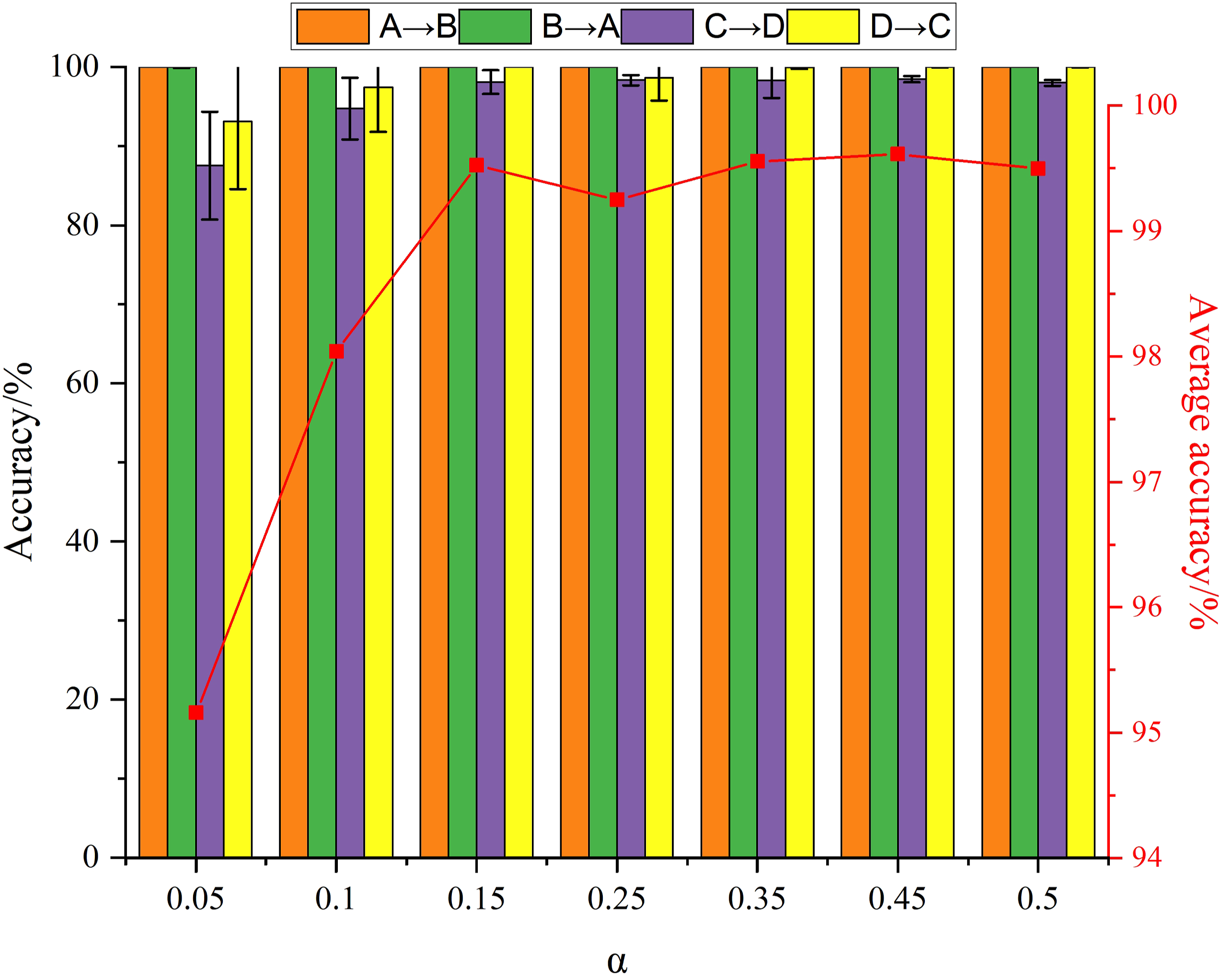

Supposing that all samples in the target domain participate in training, β is the ratio of samples participating in training to the total samples in the source domain. β is taken as 5%, 15%, 25%, 35%, 45%, and 50% in the source domain for training. Figure 6 shows that the accuracy of all tasks is higher than 90%, and task C → D is greatly affected by β. Compared with the accuracy and variance of the other three tasks, task C → D has the lowest accuracy and larger variance. When β increases, the average accuracy decreases slightly, but it is much higher than 99%.

Figure 6.

The effect of training sample size from source domain on results.

In general case, only part of samples in both source domain and target domain participated in training, α = {5%, 15%, 25%, 35%, 45%, 50%, 100%} and β = {5%, 15%, 25%, 35%, 45%, 50%, 100%}; the average accuracy and variance of the four tasks under different parameter combinations are shown in Figure 7.

Figure 7.

The effect of training sample size from source domain and target domain on results: (a) accuracy and (b) variance.

The transition color in Figure 7 (a) brightens from the lower left corner to the upper right corner. The color of upper right corner in Figure 7 is lighter, which indicates that increasing the training sample size of source and target domains at the same time will significantly improve the accuracy of the model and ensure the stability of the results. The reason for this phenomenon is that increasing the training sample simultaneously can enhance the generalization ability of the model. Figure 7 (b) shows that the transition color darkens from the upper left corner to the lower right corner with the largest variance in the lower right corner. Correspondingly, the lower right corner in Figure 7 (a) has the darkest color and the lowest accuracy, which indicates that reducing the training sample size of the target domain while increasing the training sample size of the source domain will lead to instability of the result and decline of the detection accuracy because only increasing the training samples in the source domain will strengthen the supervised learning ability of the model to the classification knowledge, but weaken the unsupervised learning ability of the transfer knowledge, and then further weaken the generalization ability of the model. In addition, it can be seen intuitively from Figure 7 that most areas are light-colored, indicating the model has high accuracy under the combination of most sample sizes, and the model has good performance.

4.6. The influence of noise in the target domain on the result

This section discusses the detection accuracy of the current method under a noisy environment. In a real industrial scenario, researchers can perform pre-processing on the source domain data such as noise reduction or feature enhancement to improve the quality, while the target domain data may contain a lot of noise. Different degrees of Gaussian noise are added to the original target domain data in order to approximating the actual data. The definition of signal-to-noise ratios is as follows

SNR = 10 \log_{10} (\frac{P_{signal}}{P_{noise}})

(19)

where

P_{signal}

and

P_{noise}

are the power of signal and noise, respectively.

Figure 8 shows the accuracy of different transfer tasks under different signal-to-noise ratios. It shows that when the signal-to-noise ratio is high, the classification accuracy of all tasks is very high. When SNR ≥ 2 dB, the average accuracy will exceed 99%, and the accuracy of C→D is the lowest, but it is also higher than 98%. When SNR is less than or equal to 0 dB, the accuracy of C→D drops significantly, lower than 90%.

Figure 8.

The effect of SNR.

5. Why works?

In order to quantify the distribution differences between two domains, α-distance (Ben-David et al., 2010) is generally adopted to estimate the difference between different distributions

A (Δ_{s}, Δ_{t}) = 2 (1 - 2 err (h))

(20)

where

err (h)

represents the hinge loss of the linear classifier and the linear classifier is trained to distinguish features from the source domain or the target domain. The smaller the value of α-distance is, the smaller the difference is. In this article, linear support vector classifier will be adopted.

Figure 9 shows the α-distance values of different methods and the proposed method in this article on different tasks. It shows that the α-distance value of the proposed method is the smallest, which is significantly lower than the values of other methods. It indicates that if the extracted features both from the source domain and target domain are very similar, the linear classifier is difficult to distinguish domain features. TICNN and ResNet have the worst performance on tasks because α-distance value of them is the highest. This indicates that the extracted features are not similar and are easily distinguished by linear classifiers.

Figure 9.

α-distance on different task.

The features of network learning are clustered and displayed by the t-SNE algorithm (Van der Maaten and Hinton, 2008). Taking task C→D as an example, as shown in Figure 10. Figure 10 (a) shows the source and target domain features distribution scatter diagram extracted by this method. It can be seen from Figure 10 (a) that the category features are well separated, with almost no overlap, and the feature scatters of the same category from source domain and target domain are almost overlapped. It can be seen from Figure 10 (b)–(e) that the feature scatters in the source domain are well separated, but the features in the target domain are not well separated, and the features of the target domain and the source domain do not overlap. It can be seen from Figure 10 (f) that the feature scatters of source domain and target domain are well separated, and only littles of samples overlap on the source domain.

Figure 10.

Feature visualization via t-SNE on task C→D: (a) ours, (b) TICNN, (c) ResNet, (d) TCA, (e) JDA, and (f) DDC.

Taking task C → D as an example, the feature map of last convolutional layer for dataset D is extracted, as shown in Figure 11. It shows only a few bright color bands on the feature spectrum of the four categories, which means that the features extracted by the neural network are sparse. From the perspective of signal analysis, the method based on deep learning transforms the fault signal from the original space to a new space in the training process. In the new space, if the signal has only a small amount of non-zero values, it is sparse in this new space, and this space is named a good sparse domain. The sparsely expressed features will improve the robustness of the model.

Figure 11.

Feature map of the last convolution layer: (a) health, (b) roller fault, (c) inner fault, and (d) outer fault.

6. Conclusion

Aiming at diagnosing bearing faults, a method based on local joint distribution discrepancy is proposed in this article to increase similar features. And a sub-domain adaptive transfer learning method is designed based on the residual network. This article studies the transfer learning of bearings under different working conditions and different fault degrees and studies the fault transfer learning of different types of bearings. The results show that compared with other methods, the method proposed achieves the highest accuracy in various tasks. The influence of noise and training sample size on the proposed method is further studied. The results show that the method has a certain anti-noise ability and good generalization ability.

Footnotes

Declaration of conflicting interests

The author(s) declared no potential conflicts of interest with respect to the research, authorship, and/or publication of this article.

Funding

The author(s) disclosed receipt of the following financial support for the research, authorship, and/or publication of this article: The authors gratefully acknowledge the financial support by the 111 Project P.R.China (Grant No. B16038).

ORCID iD

Di Zhang

References

Ben-David

Blitzer

Crammer

, et al. (2010) A theory of learning from different domains. Mach. Learn 79(1–2): 151–175.

Cerrada

Sánchez

R-V

, et al. (2018) A review on data-driven fault severity assessment in rolling bearings. Mechanical Systems and Signal Processing 99: 169–196.

Cheng

Zhou

, et al. (2020) Wasserstein distance based deep adversarial transfer learning for intelligent fault diagnosis with unlabeled or insufficient labeled data. Neurocomputing 409: 35–45.

Ganin

Ustinova

Ajakan

, et al. (2015) Domain-adversarial training of neural networks. Computer Science 17: 1–35.

Guo

Lei

Xing

, et al. (2019) Deep convolutional transfer learning network: a new method for intelligent fault diagnosis of machines with unlabeled data. IEEE Transactions on Industrial Electronics 66(9): 7316–7325.

Hoffer

Hubara

Soudry

(2017) Train longer, generalize better: closing the generalization gap in large batch training of neural networks. Advances in Neural Information Processing Systems 30: 1731–1741.

Ince

Kiranyaz

Eren

, et al. (2016) Real-time motor fault detection by 1-D convolutional neural networks. IEEE Transactions on Industrial Electronics 63(11): 7067–7075.

Jiang

Yan

, et al. (2019) Multiscale convolutional neural networks for fault diagnosis of wind turbine gearbox. IEEE Transactions on Industrial Electronics 66(4): 3196–3207.

Jiao

Zhao

Lin

, et al. (2020) Residual joint adaptation adversarial network for intelligent transfer fault diagnosis. Mechanical Systems and Signal Processing 145: 106962.

10.

Kaiming

Xiangyu

Shaoqing

, et al. (2016) Deep residual learning for image recognition. In: 2016 IEEE Conference on Computer Vision and Pattern Recognition (CVPR), Las Vegas, NV, 27-30 June. DOI: 10.1109/CVPR.2016.90.770-778

11.

Kingma

(2014) Adam: a method for stochastic optimization. Computer Science.

12.

Lei

Yang

Jiang

, et al. (2020) Applications of machine learning to machine fault diagnosis: A review and roadmap. Mechanical Systems and Signal Processing 138: 106587.

13.

Zhang

Qin

, et al. (2020a) A systematic review of deep transfer learning for machinery fault diagnosis. Neurocomputing 407: 121–135.

14.

Zhang

, et al. (2020b) Partial transfer learning in machinery cross-domain fault diagnostics using class-weighted adversarial networks. Neural Networks 129: 313–322.

15.

Chu

Han

(2019) Deep residual learning with demodulated time-frequency features for fault diagnosis of planetary gearbox under nonstationary running conditions. Mechanical Systems and Signal Processing 127: 190–201.

16.

Mingsheng

Jianmin

Jordan

(2016) Deep Transfer Learning with Joint Adaptation Networks [arXiv]. arXiv. 10 pp.

17.

Pan

S. J.

Yang

(2010) A survey on transfer learning. Ieee Transactions on Knowledge and Data Engineering 22(10): 1345–1359.

18.

Qiu

Lee

Lin

, et al. (2006) Wavelet filter-based weak signature detection method and its application on rolling element bearing prognostics. Journal of Sound and Vibration 289(4–5): 1066–1090.

19.

Smith

Randall

(2015) Rolling element bearing diagnostics using the Case Western Reserve University data: A benchmark study. Mechanical Systems and Signal Processing 64-65: 100–131.

20.

Tong

Zhi

Hang

, et al. (2019) Bag of tricks for image classification with convolutional neural networks. In: 2019 IEEE/CVF Conference on Computer Vision and Pattern Recognition. Long Beach, CA, pp. 558–567.

21.

van der Maaten

Hinton

(2008) Visualizing data using t-SNE. Journal of Machine Learning Research 9: 2579–2605.

22.

Wang

Xie

Zhang

(2021) Deep learning for bearing fault diagnosis under different working loads and non-fault location point. Journal of Low Frequency Noise, Vibration and Active Control 40(1): 588–600.

23.

Wen

Gao

(2019) A new deep transfer learning based on sparse auto-encoder for fault diagnosis. IEEE Transactions on Systems, Man, and Cybernetics: Systems 49(1): 136–144.

24.

Jiang

, et al. (2020) A deep transfer maximum classifier discrepancy method for rolling bearing fault diagnosis under few labeled data. Knowledge-Based Systems 196: 105814.

25.

Yang

Lei

Jia

, et al. (2019) An intelligent fault diagnosis approach based on transfer learning from laboratory bearings to locomotive bearings. Mechanical Systems and Signal Processing 122: 692–706.

26.

Zhang

Peng

, et al. (2018) A deep convolutional neural network with new training methods for bearing fault diagnosis under noisy environment and different working load. Mechanical Systems and Signal Processing 100: 439–453.

27.

Zhang

Ding

(2019) Deep residual learning-based fault diagnosis method for rotating machinery. Isa Transactions 95: 295–305.

28.

Zhao

Yan

Chen

, et al. (2019) Deep learning and its applications to machine health monitoring. Mechanical Systems and Signal Processing 115: 213–237.

29.

Zhu

Hou

Zhou

, et al. (2019) Rotor fault diagnosis using a convolutional neural network with symmetrized dot pattern images. Measurement 138: 526–535.

30.

Zhu

Zhuang

Wang

, et al. (2021) Deep subdomain adaptation network for image classification. IEEE Transactions on Neural Networks and Learning Systems 32(4): 1713–1722.