
Abstract
The fuzzy set theory for optimal control design of underactuated dynamical systems with uncertainty is proposed. The uncertainty is (possibly fast) time varying whose bound is unknown and lies in a prescribed set expressed by a fuzzy set. Control goals of uncertain dynamical systems are formulated as a series of constraints, which may be holonomic and nonholonomic. From the view of constraint-following control, we design an adaptive robust control based on a creative uncertainty decomposition, which divides the uncertainty into matched and mismatched terms. This decomposition renders the mismatched term to “disappear” in the stability analysis. The proposed control is able to drive the system to approximately follow the constraints and guarantee system performance (uniform boundedness and uniform ultimate boundedness), in the presence of the uncertainty. It is in deterministic form and not “if–then” fuzzy rules based. Because of the expressed fuzzy set of the uncertainty bounds, a performance index, which balances the conflict between system performance and control cost, can be constructed. An optimal design gain can be obtained by minimizing the performance index whose solution is guaranteed to always exist. Numerical results on a planar vertical takeoff and landing aircraft are presented for demonstration.
Keywords
1. Introduction
Because underactuated systems extensively exist in the engineering practice, servo control design for underactuated systems has been a hot spot issue in recent years (Chen and Sun, 2019; Kant et al., 2019; Xu and Ümit, 2008; Yin et al., 2020). Research studies on the motion control of underactuated systems, such as planar vertical takeoff and landing aircraft (Castañeda et al., 2018), active suspension system (Pan and Sun, 2019), two-wheeled mobile robot (Silva and Sup, 2017), and so on, have been widely attracted by academia and industry. From the perspective of the motion control design, a salient feature of underactuated systems is that it has fewer control inputs than the degrees of freedom to be controlled. Therefore, this is a challenge problem usually encountered by researchers. Despite of the complexity, there are various control approaches considering this issue from different angles (Liu et al., 2019; Mobayen, 2019). However, the problem of the control design for underactuated systems still needs new development and more insight. The purpose of this study is to contribute to addressing this problem.
In real-world systems, uncertainty always exist in practical underactuated dynamic systems (Azimi and Koofigar, 2015; Hwang et al., 2013; Roy and Baldi, 2020), such as parameters, external disturbance, and so on, which may significantly influence the system performance. Therefore, it is necessary to consider the uncertainty when designers design control strategies. In general, if the bound of uncertainty in underactuated systems is known, a robust control can be designed to ensure the system performance (Petersen and Tempo, 2014; Yang et al., 2019). During the design process of robust control, the uncertainty set must cover all the possible values, and the bound of uncertainty can be defined. Therefore, the defined bound may be too large and thus be rather conservative, which may lead to obtain an unnecessary high control gain. On the contrary, an adaptive robust control does not need the known bound of the uncertainty (Chen et al., 2019; Sun et al., 2018a, 2018b). Generally, the bound can be emulated by constructing an adaptive law (e.g., leakage law), which aims to avoid generating a high control gain. The adaptive robust control can effectively deal with the unknown bound of the time-varying uncertainty in underactuated systems.
As for the unknown bound of time-varying uncertainty, researchers can collect a certain amount of data to design the special distribution function for describing the unknown bound. The distribution function can be used for optimal design of an adaptive robust control and constructed by a particular uncertainty theory. The probability theory is famous for handling this issue (Durrett, 2010). It expresses the bound of uncertainty by the frequency occurrence. From the 1950s, the integration between the probability theory and the dynamic systems occurs, which is called stochastic dynamical system. Many researchers have worked for its development and achieved great success (Haddad et al., 2019; Rajpurohit and Haddad, 2016; Rajpurohit and Haddad, 2017). However, there exist some criticisms about the probability theory. The main contention is that the probability theory is precisely constructed on the basis of obtaining a large amount of data, whereas it is very hard to complete such task in the engineering practice (Adhikari and Khodaparast, 2014). To solve the above problem, the fuzzy set theory can be selected and used for describing the unknown bound of uncertainty.
In 1965, Zadeh (1965) proposed the fuzzy set theory, which is not a fuzzy logic theory. The fuzzy set theory is different from the probability theory. It expresses the uncertainty by the degree of occurrence and focus on indicating the vague information such as “Jim’s age is close to 18 years old.” Therefore, the fuzzy theory does not involve collecting a large amount of data but is determined by the professional experience. Until now, the fuzzy theory has been widely used for expressing the uncertainty and successfully applied in various fields (Maues et al., 2020; Taylan et al., 2016). For the control field, the fuzzy set theory is less well known than the fuzzy logic control theory which is based on the “if–then” fuzzy rules (Gu et al., 2019). Fortunately, many researchers have carried out some constructive work about applying the set theory for the full actuated dynamical systems. For example, Chen (2001), (2011) pioneered to investigate the merger between the fuzzy set theory and the full actuated dynamical systems; Huang et al. (2015) explored the integration between an adaptive robust control and the fuzzy set theory for full actuated systems from the avenue of the constraint-following control.
The constraint-following control initiated based on the Udwadia–Kalaba (U–K) approach is well known for its capability to handle both holonomic and nonholonomic constraints in mechanical systems (Chen, 2009). It is also accompanied with advantages, such as not requiring any system linearizations or nonlinear cancellations, or any auxiliary variables (such as Lagrange multiplier), or pseudo variables (such as generalized speeds), rendering the control force to satisfy Gauss’s minimum principle and the Lagrange’s form of d’Alembert’s principle (hence exhibiting a modest control magnitude in practice). These advantages inspire some researchers to keep exploring an adaptive robust control for full actuated systems, in which uncertainty bound is described by the fuzzy set, from the avenue of constraint-following control (Xu et al., 2015; Zhao et al., 2016). However, there are few research studies on applying the fuzzy set theory in underactuated dynamical systems for optimal control gain from the view of the constraint-following control. Therefore, it is promising to call for more explorations.
The main contribution of this study is to apply the fuzzy set theory to design an adaptive robust control based on the constraint-following control and obtain optimal control gain for underactuated dynamical systems with uncertainty. The uncertainty is (possibly fast) time varying whose bound is unknown and lies in a prescribed set expressed by a fuzzy set. It should be emphasized that the fuzzy numbers in the fuzzy set are all crisp. The control design is implemented in three steps. First, we formulate the control goals of underactuated dynamical systems as a class of constraints, which may be holonomic and nonholonomic. According to constraints and the structure of systems, a creative uncertainty decomposition is proposed to ensure the mismatched portion to “invisible,” which can be taken advantage of the stability analysis. Second, based on the constraint-following control, an adaptive robust control for underactuated dynamical systems is designed, in which a smooth-zone adaptive law of leakage type is constructed. The control is deterministic and is not “if–then” fuzzy rules based. The uniform boundedness (UB) and uniform ultimate boundedness (UUB) of underactuated dynamical systems under the proposed control are rigorously proved, which indicates that the approximate constraint-following is guaranteed. Third, the optimal control design can be achieved by using the fuzzy set numbers that describe the bound of uncertainty. Specifically, the combined cost, including the average system performance described by fuzzy numbers and control effort, is designed to be minimized by an appropriate choice of the control gain. This is formulated as a constrained optimal design problem, whose solution is guaranteed to always exist. Numerical simulation results on a planar vertical takeoff and landing aircraft are presented for verification.
2. Basic of fuzzy set theory
The fuzzy set can be regarded as a generalization of the conventional set (Chen, 2011). In the scenario of the conventional set, an element is either “totally belonging to” or “totally not belonging to” the set. However, an element can be “possibly belonging to” the set in the scenario of the fuzzy set. In general, a fuzzy set

In general, the fuzzy set
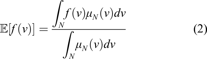
Consider a fuzzy number described as (1). For any function f: N →
Lemma 1For any crisp constant a ∈ The proof of Lemma 1 and some other properties of fuzzy numbers are presented in Appendix (Chen, 2011).

3. Uncertain underactuated system subject to constraints
Consider the dynamical model of underactuated systems with uncertainty as follows
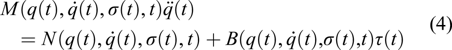
Here, t ∈
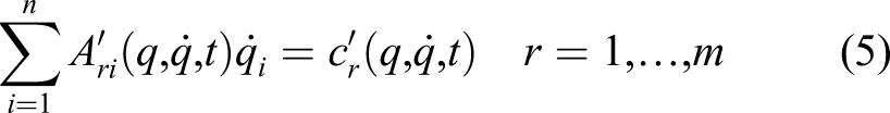
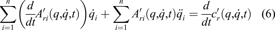
The displacement q can be selected as generalized coordinate. The matrices N(⋅) and B(⋅) are continuous. Now, we formulate control goals of dynamical systems as the following first-order form constraints (Yin et al., 2020) To obtain the second-order form of constraints (5), we take derivative of (5) with respective to t, and the following is obtained Because Furthermore, the first-order form of constraints, that is, (5), can be rewritten as


The proposed constraints in (15) are different from those in Chen (2009), which cover the velocity vector
Definition 1For given Γ and ϒ, the equation ΓΛ = ϒ is called consistent if there exists at least one solution Λ.
Constraint (12) is consistent with respect to
3.1. Adaptive robust servo control design
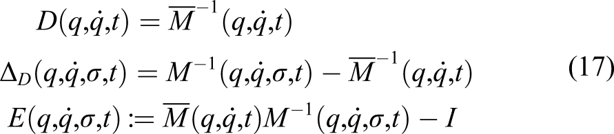
Now, we decompose the matrices M, N, and B in (4) as follows
For all Let We obtain We decompose E based on E is decomposed into two portions: the matched portion The uncertain portion Δ
B
is decomposed based on


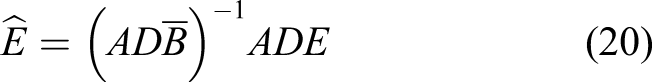
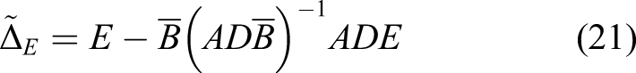
Let

To prove (22), we take the case
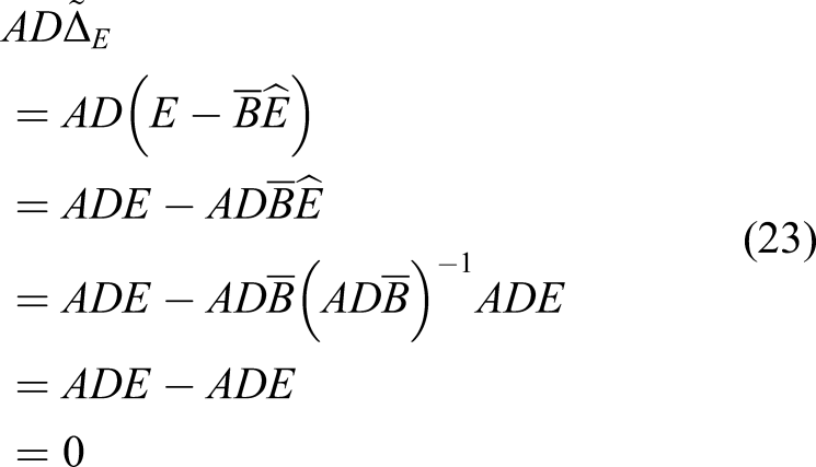
By (22), the above uncertainty decomposition ((20) and (21)) creatively assigns the mismatched uncertain portions to be within the null space of AD. Consequently, the mismatched portions are always invisible, and only the matched portions in the range space of AD are in question. As A and D are, respectively, related to the constraints and the system, this decomposition in a sense is based on the structure of the system and constraints. It will be used in later development.
Based on Assumption 2, for given positive definite matrix G ∈ There exists a constant ρ
E
≥ −1 such that for all q ∈ Ω
q
,
If there is no uncertainty in M, that is,
Let, We now construct the control as Here The estimated parameter
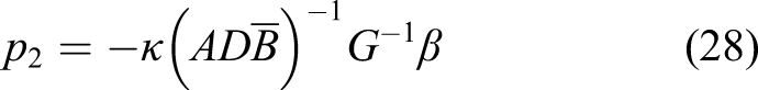


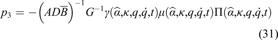
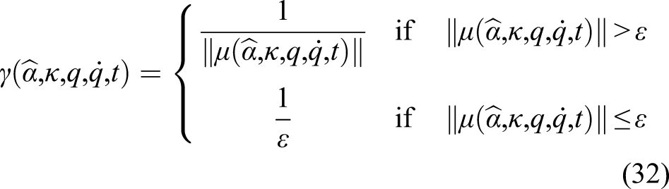

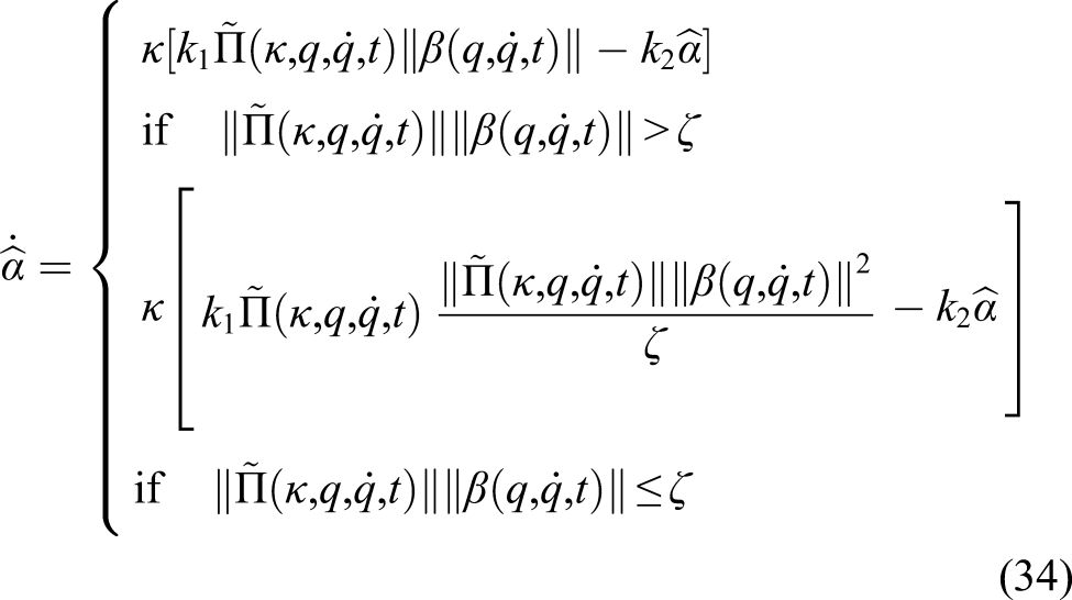
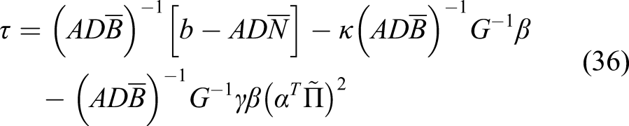
Compared with the dead-zone adaptive law, the proposed adaptive law is continuous at the critical point. Therefore, we call it the smooth-zone adaptive law. The first terms on the RHS of (34) intend to emulate the increase of By using (27)–(29), (31), and (33), the control input (30) can be rewritten as By (36), the proposed control is a model-based state feedback control. The control input τ is determined by the constraint matrix (i.e., A) and the dynamical model (i.e.,
Consider the dynamical systems (4) and let Uniform boundedness: For any r > 0, there is a d(r) < ∞ such that if ||δ(t0)|| < r, then ||δ (t)|| ≤ d(r) for all t ≥ t0; Uniform ultimate boundedness: For any r > 0 with ||δ(t0)|| < r, there exists a
See the Appendix 1.
From the analysis in the proof (see the Appendix 1), we can find that the proposed control can enable the uniform boundedness and the uniform ultimate boundedness of dynamical systems subject to uncertainties and constraints, which may be holonomic or nonholonomic. From (90)–(93), it can be found that the control parameter κ affects the size of the uniform boundedness and the uniform ultimate boundedness, which is associated with the system performance. On the other hand, κ also influences the control cost. This indicates a trade-off between the system performance and the control cost. Because the fuzzy sets describing the uncertainty bounds are available, it is possible to address the trade-off by optimal design considerations with utilization of them.
4. Optimal gain design
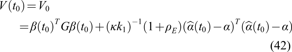
4.1. Performance index for the optimal gain design
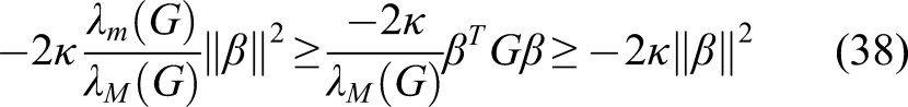
By Rayleigh’s principle, we yield

Because λ
m
(G) > 0, we can obtain
From (86)–(88), we have

By Hale (1969), the corresponding differential equation of (41) is

The solution of (43) can be described as
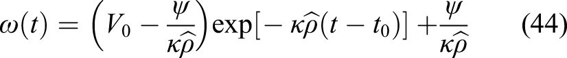
Based on the theory of differential inequality, we can get

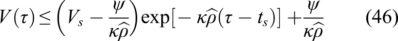
By (37), we can find
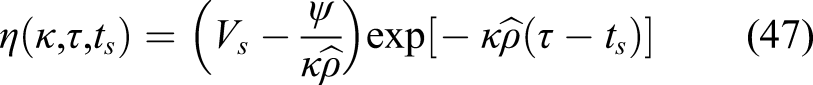
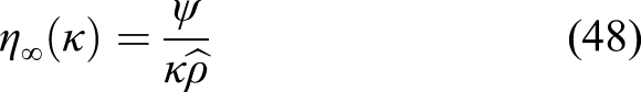
It can be found that for any given κ and t
s
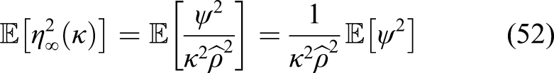
, η(κ, τ, ts) → 0 as τ → ∞. We propose the performance index as follows: for any t
s
, let
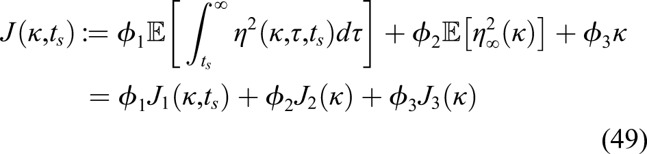
Considering the first term on the RHS of (49), we have
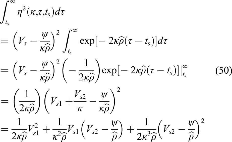
Therefore
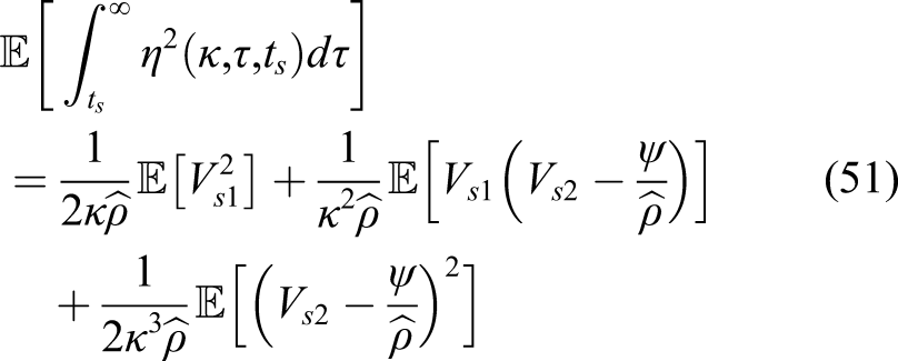
Considering the second term on the RHS of (49), we have
Based on (49), (51), and (52), we obtain
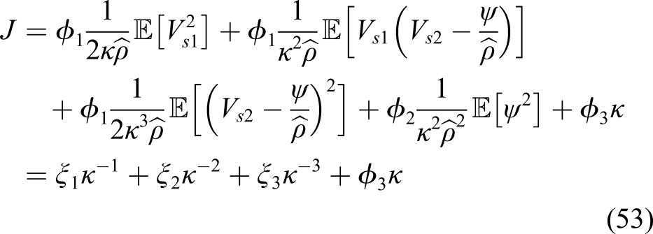
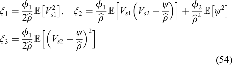
The optimal gain design problem can be described as the following constrained optimization problem: for any t
s

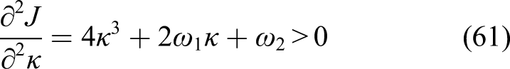
By (52), it can be found that (1) J can be viewed as a continuous function of κ on (0; + ∞); (2) J > 0; and (3) J → + ∞ as κ → 0+ or κ → + ∞. Therefore, we can conclude that the minimum of J always exists by the property of continuous functions, that is, the solution of (55) always exists. How to obtain the solution of (55) will be presented as follows.
4.2. Solution of the optimal gain design
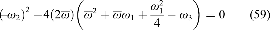
The solution of the constrained optimization problem (55) belongs to the set of roots of the following the equation

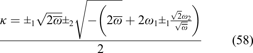
Denote the four roots of (55) in (58) as κ1,2,3,4. Based on the discussions in the last paragraph, we can conclude that there is at least one positive real root among κ1,2,3,4. As ω3 < 0, we can further conclude that there may be one or three positive real roots among κ1,2,3,4. By the property of the roots of quartic equations, we make the following discussions. In the case that there is only one positive real root among κ1,2,3,4, the other three roots may be all negative real numbers or one negative real number with two conjugate complex numbers. Denote the only one positive real root as κopt+; then, the solution of the constrained optimization problem (55) is 2. In the case that there are three positive real roots among κ1,2,3,4, the other root is a negative real number. Among the three positive real roots, there exists at least one root satisfying

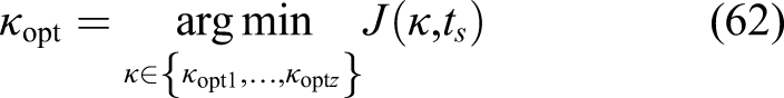
Suppose that there are z roots with 1 ≤ z ≤ 3 satisfying (61) and denote them as κopti (i = 1, …, z). Then, the solution of the constrained optimization problem (55) is
5. Illustrative example
A planar vertical takeoff and landing aircraft, which is shown in Figure 1, is used for demonstrating the proposed control approach. The dynamical equation of normalization parameter can be expressed as (Hauser et al., 1992) Planar vertical takeoff and landing aircraft.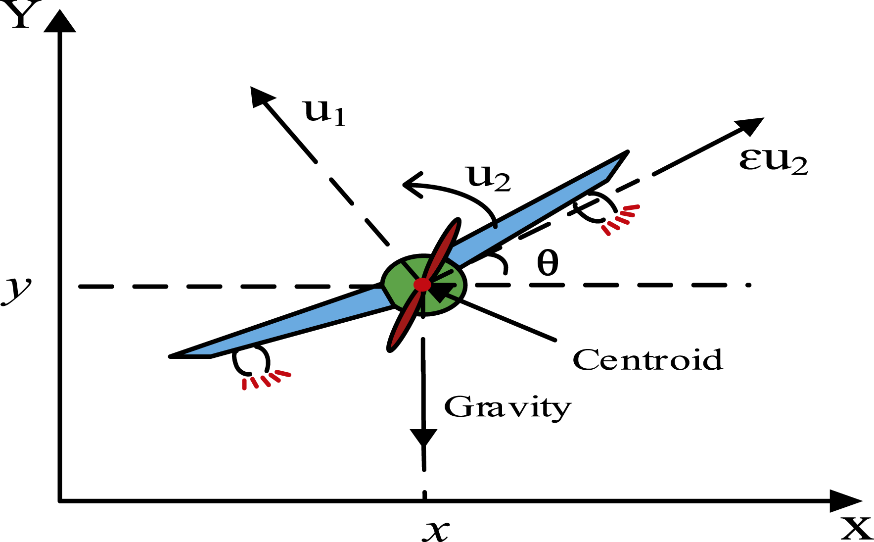
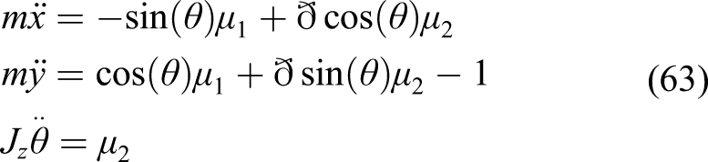
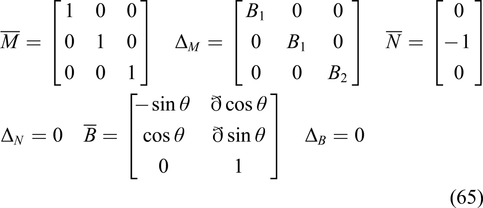
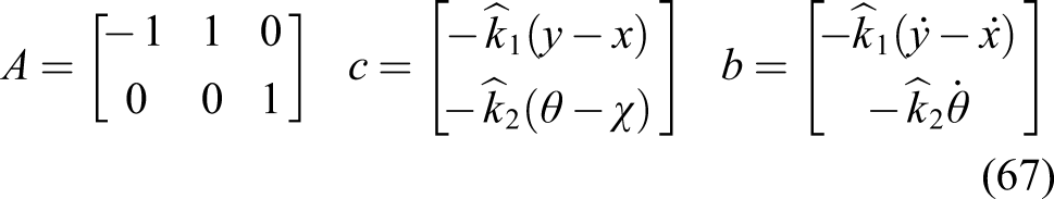
Equation (63) can be cast into the form of (4) by letting
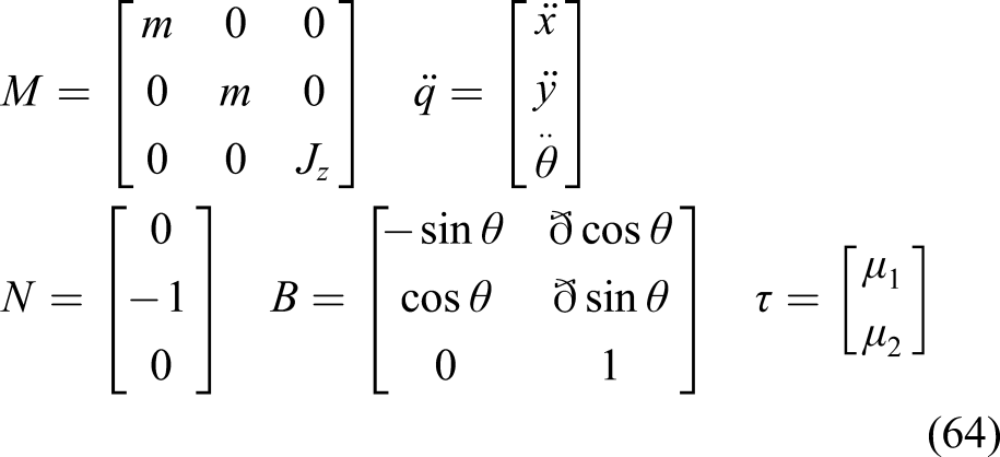
Suppose that there exist uncertainties in m and J
z
, and the nominal values of them are 1 kg and 1 kg ⋅m2. Then, m and J
z
can be decomposed as m = 1 + B1 and J
z
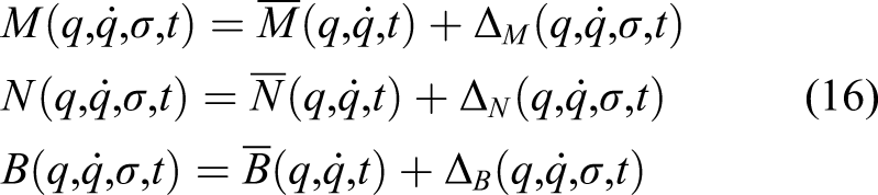
= 1 + B2, where B1 and B2 are the time-varying uncertainties. These uncertainties are bounded as |B1| ≤ B1m and |B2| ≤ B2m with B1m and B2m unknown constants but lying within the prescribed fuzzy numbers. M, N, and B can be decomposed into the form of (16) by letting
Suppose that the following constraints are imposed on the motion of a planar vertical takeoff and landing aircraft

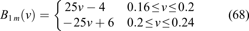
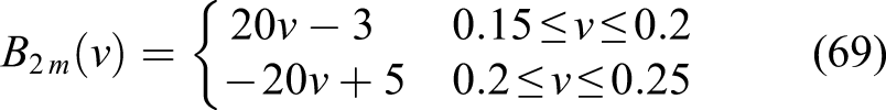
The unknown bounds of B1m and B2m lie within the following fuzzy numbers. The fuzzy (linguistic) descriptions of B1m and B2m are expressed as “B1m and B2m are close to 0.2.” The corresponding membership functions for B1m and B2m are (all triangular)
For simulation, we select G = I, ζ = ɛ = 0.5, k1 = k2 = 1,
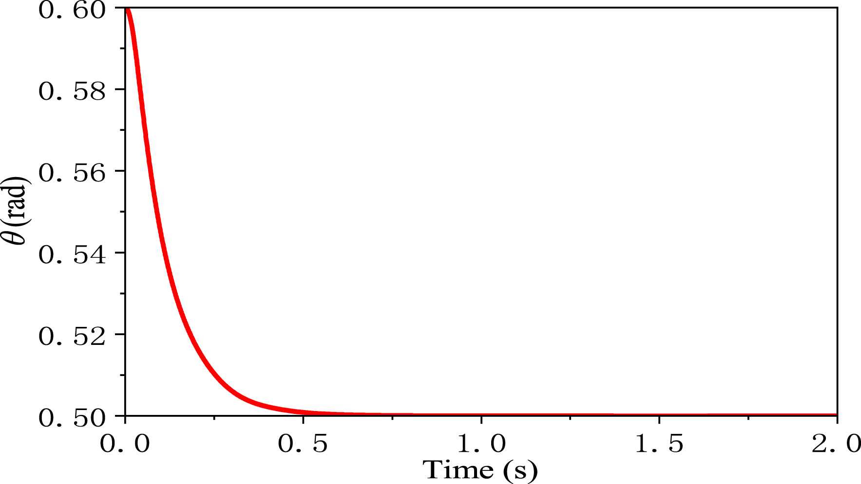
Figure 2 and Figure 3 show the horizontal position, the vertical position, and the angle with respect to the time under the proposed control. It can be found from Figure 2 and Figure 3 that the system of the planar vertical takeoff and landing aircraft meets the constraint (66) in finite time under the effect of the uncertainty. Horizontal and vertical positions with respect to the time under the proposed control. Angle with respect to the time under the proposed control.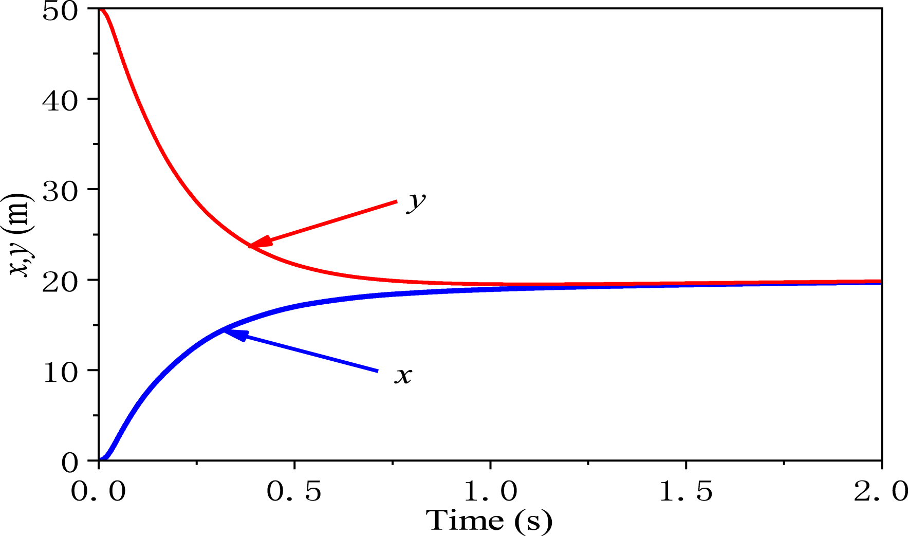
To show the merit of the proposed control, the sliding mode control (Aguilar-Tbanez, 2016) is selected for comparison, which is well known for the capability of handling the model error and parametric uncertainties. It is designed and based on a simple feedback linearization procedure in combination with a saturation function. The selected control parameters for the sliding mode control only guarantee the locally asymptotically stable, which is not obtained by the optimal design.
The constraint-following error ||β(t)|| is used for indicating the system performance. Figure 4 shows the ||β(t)|| histories under no control, the sliding mode control, and the proposed control (under κopt = 4.5835 when using ϕ1 = ϕ2 = 1, ϕ3 = 0.25). It can be found that ||β(t)|| history under no control is far from 0, whereas ||β(t)|| histories under the proposed control and the sliding mode control converge to 0 in finite time. Furthermore, it can be found that the accumulation error of ||β(t)|| (i.e., Constraint-following error histories under no control, the proposed control, and the sliding mode control. Comparison of control input τ1 under the sling mode control and the proposed control. Comparison of control input τ2 under the sling mode control and the proposed control. Adaptive parameter history.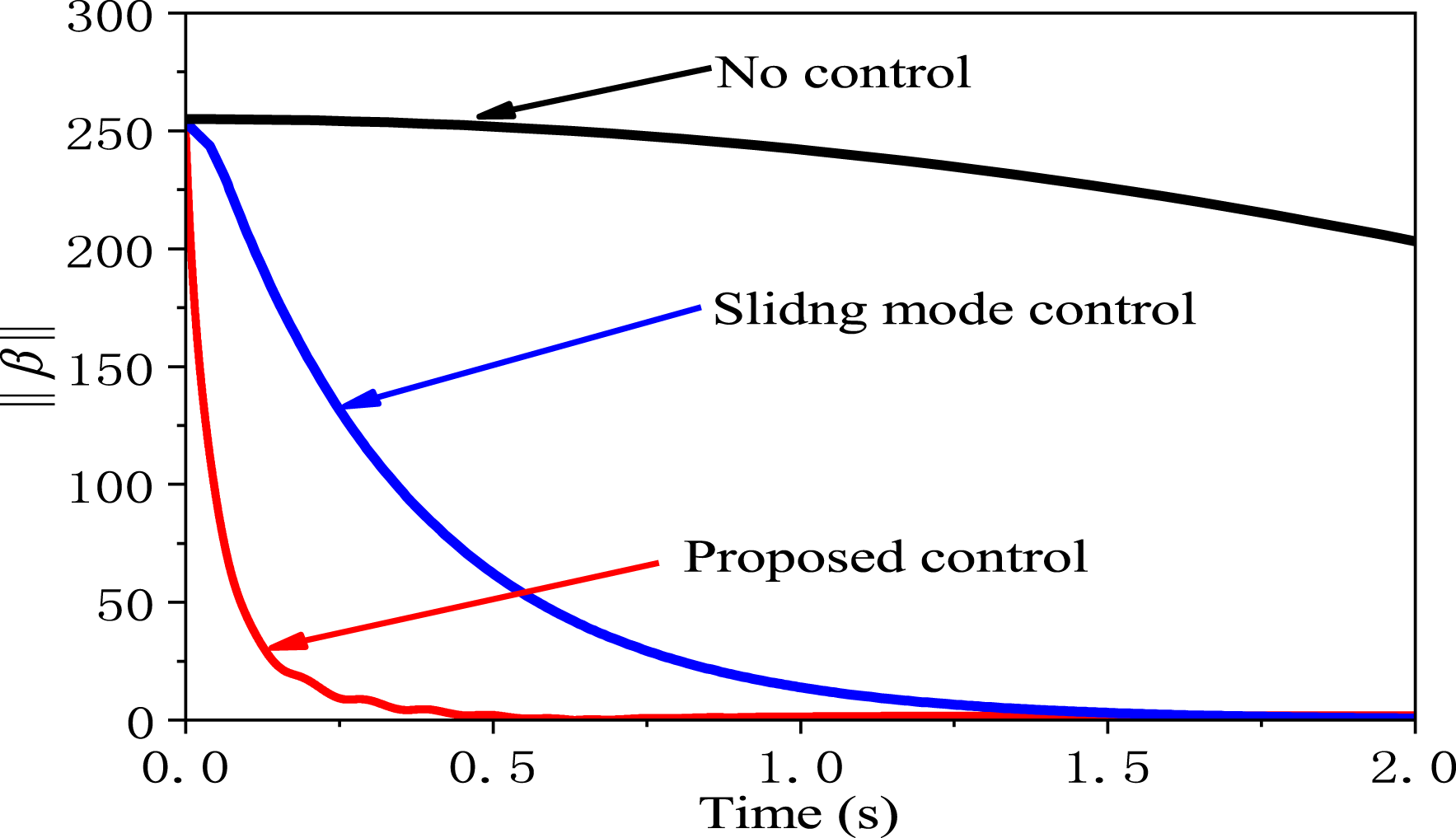
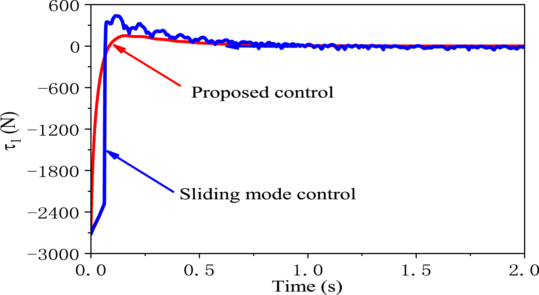
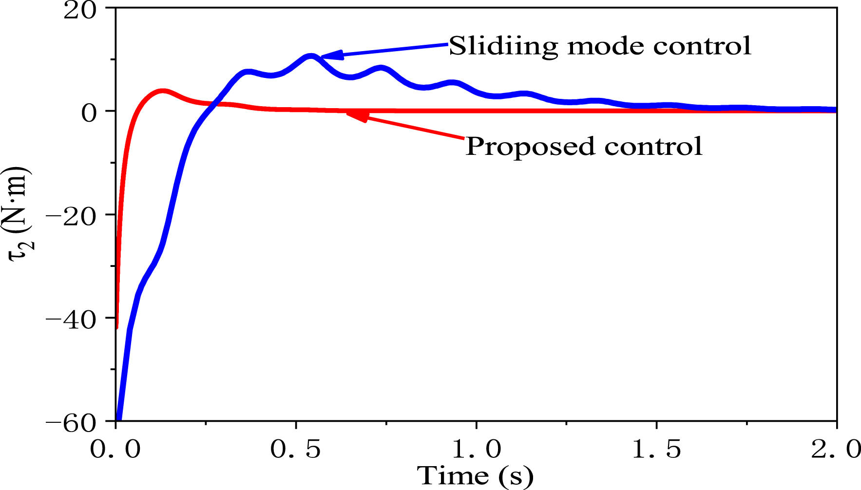
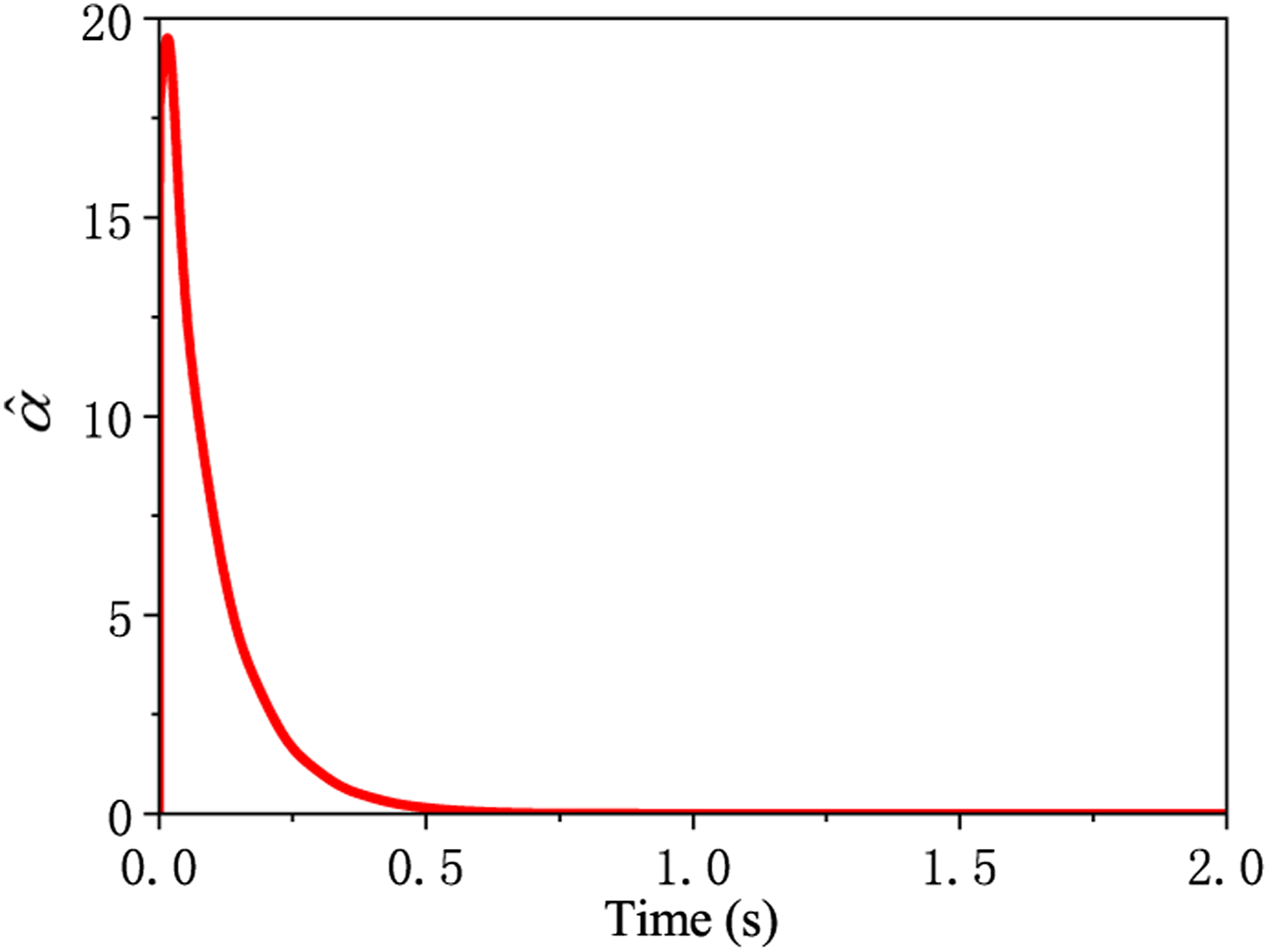
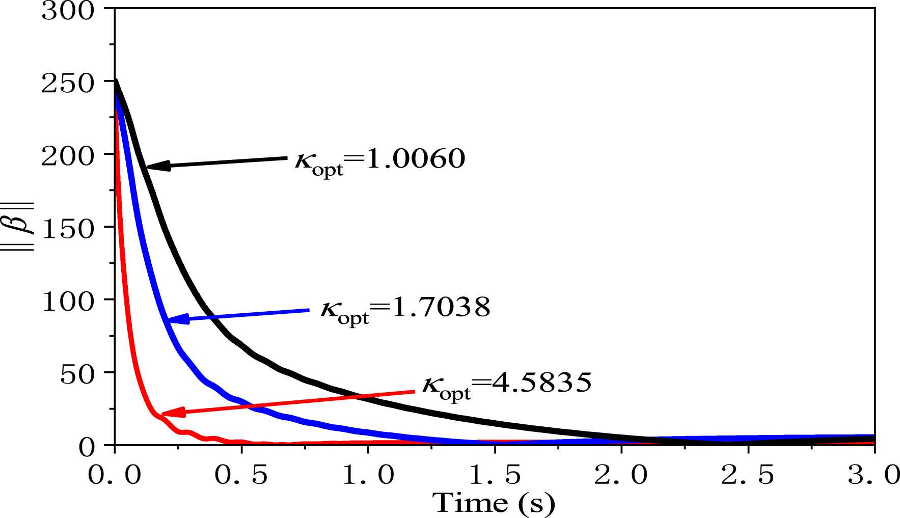
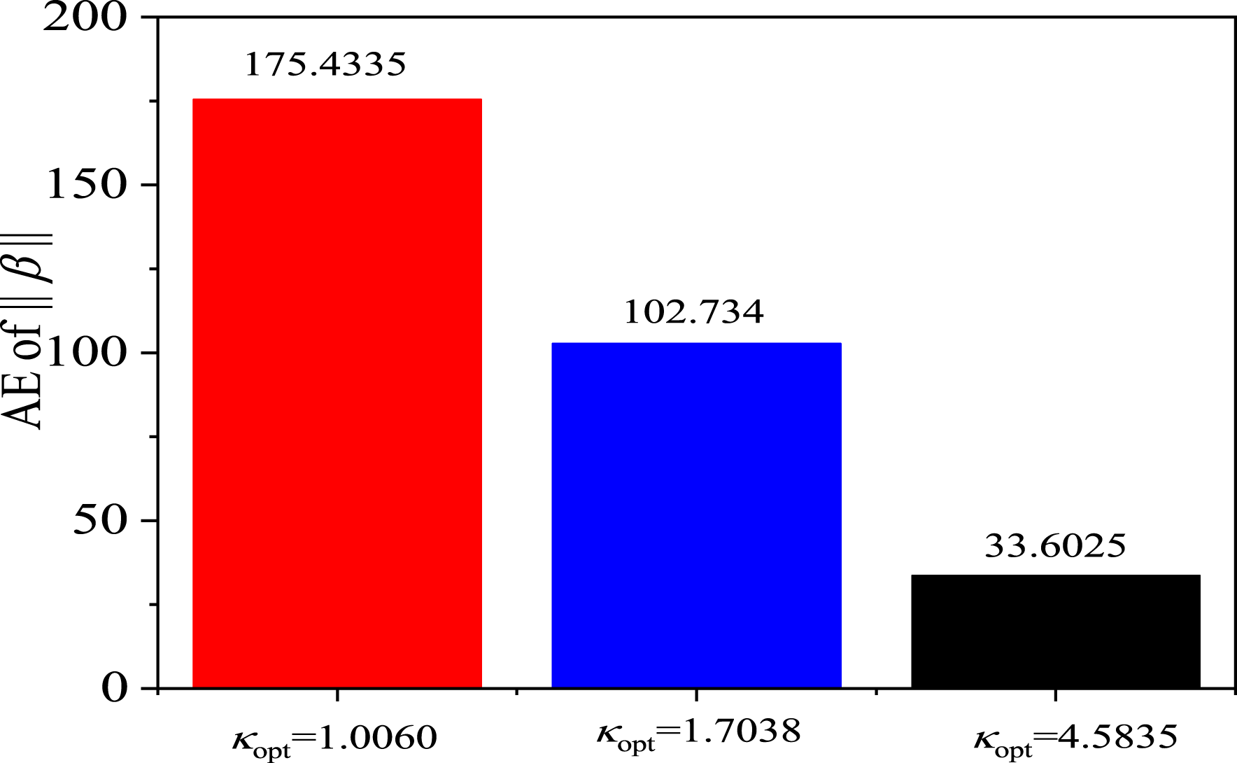
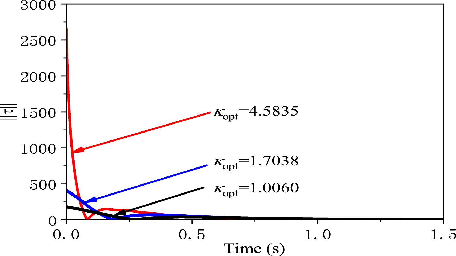
Figure 8 shows the performance index J as a function of the parameter κ under three groups of weighing factors (ϕ1, ϕ2, ϕ3). It can be found that κopt always exists and makes the performance index J minimize under three different groups of weighing factor (ϕ1, ϕ2, ϕ3). Figure 9 shows the ||β(t)|| histories under three different κopt. Figure 10 shows accumulation errors under different κopt. It can be found that the larger the κopt value, the smaller the accumulation error is. Figure 11 plots the time histories of the control efforts ∥τ∥ under three different κopt. Performance index J. Comparison of constraint-following errors under different κopt. Comparison of accumulation errors under different κopt. Comparison of control efforts under different κopt.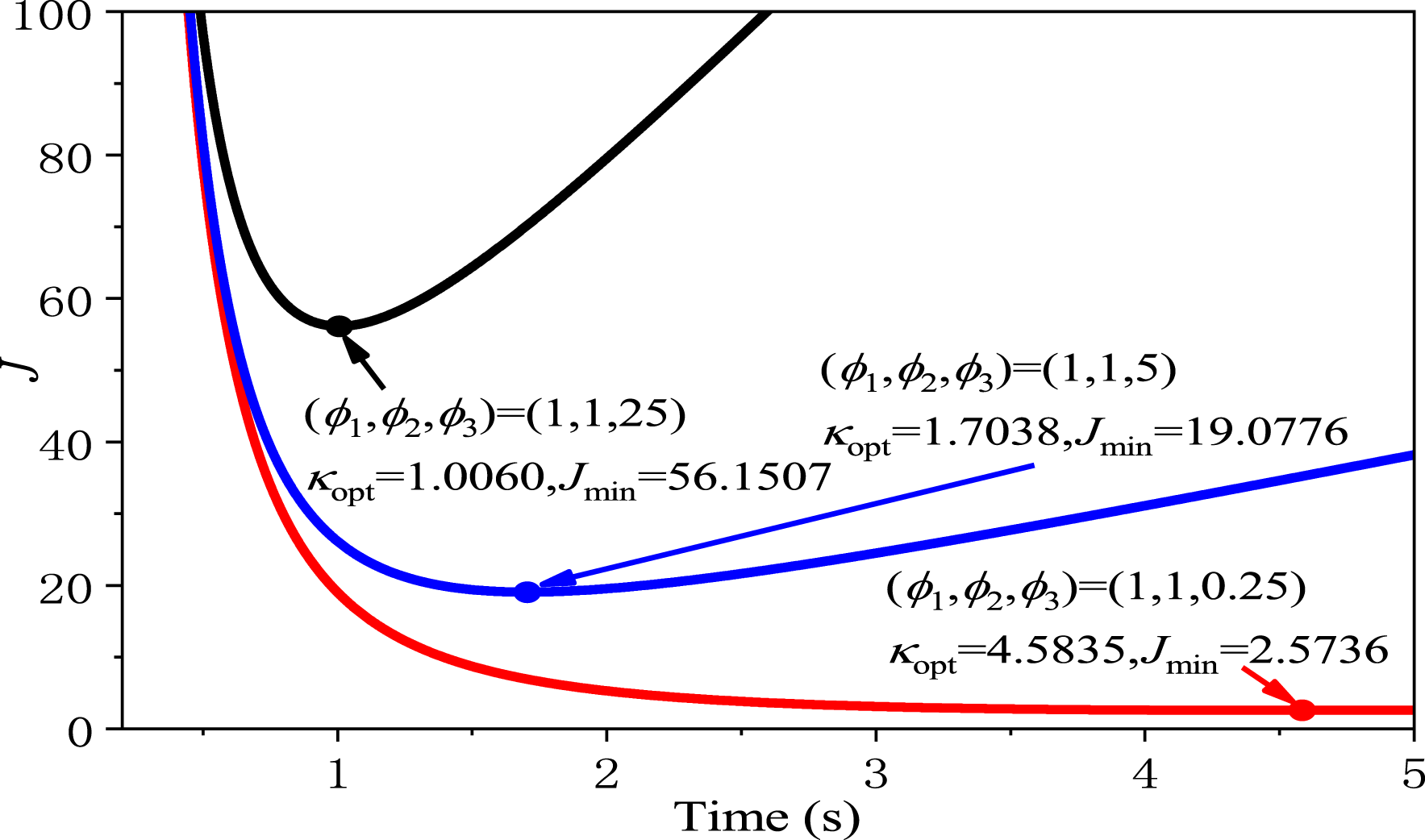
Footnotes
Declaration of conflicting interests
The author(s) declared no potential conflicts of interest with respect to the research, authorship, and/or publication of this article.
Funding
The author(s) disclosed receipt of the following financial support for the research, authorship, and/or publication of this article: The article is supported by the National Natural Science Foundation of China under Grant 51806066 and the Natural Science Foundation for Young Scholars of Jiangxi Province under Grant 20181BAB216023.
Appendix.1
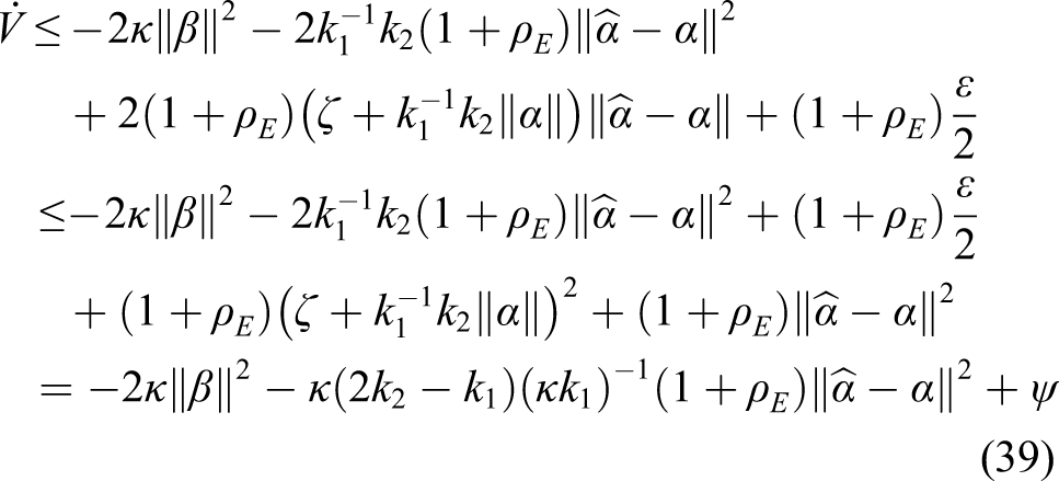
Choose the Lyapunov function candidate as
Taking derivative of V with respect to t yields (for simplicity, most of arguments of functions in this proof are omitted except for some critical ones)
By using the decompositions M−1 = D + Δ
D
and
Notice that
Based on
By applying Assumption 4 yields
Next, by (72), we have
Using
By applying Δ
D
= DE and (22), we have
According to (76)–(78), Assumption 3,
Based on (72)–(75) and (79)–(81), we can obtain, for ||μ|| > ɛ
Now, we deal with the second term on the RHS of (71) as follows. With the adaptive law ((34) and (35)), we have that if
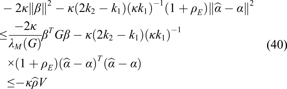
Based on (71), (84), and (87), we have
By Khalil (2002), we can obtain uniform boundedness with
Furthermore, uniform ultimate boundedness follows with