
Abstract
Due to the three-dimensional non-axisymmetric shape of the volute, its interaction with the impeller increases the internal flow field complexity and instability of the marine centrifugal pump, representing the main reason for pump body vibration and hydraulic noise. First, the basic principle of fluid machinery noise calculation was explained based on the Lighthill acoustic analogy method and Curle’s theory. Then, the fluid pressure pulsation and flow characteristics of centrifugal pumps were analyzed using the Fluent software, after which the Actran software was used to examine the flow-induced vibration noise properties. The results showed that the clearance size significantly impacted the pump head, while the peak value of the flow-induced vibration response was mainly twice the blade frequency. Although a larger ring clearance increased the structural vibration, it had little impact on the sound pressure level changes in the external sound field. The results provided a new method for the structural optimization and low-noise design of marine centrifugal pumps.
Keywords
Centrifugal pumps, widely used in marine cooling, bilge ballast, circulating water, and fire protection systems, represent the primary noise sources in marine water pipelines, significantly affecting the marine environment and safety (Wu et al., 2022). Therefore, the vibrational noise during pump operations and the stability of pump equipment have raised significant concerns.
The comprehensive simulated calculation of the internal pump flow field and related vibration and noise is essential for designing “quiet” centrifugal pumps. Studies have investigated the generation and propagation characteristics of centrifugal pump noise (Si et al., 2019). A sequential coupling method including fluid and acoustic simulation was proposed to obtain the flow-induced emitted noise characteristics. Lighthill (1952) proposed a pioneering sound analogy theory for acoustic flow issues. Goldstein (1975) studied the acoustic propagation of moving objects in a fluid medium and derived the generalized Lighthill equation. Chu et al. (1995) determined the flow field distribution in the centrifugal pump via particle displacement velocity measurements, indicating that the main reason for far-field flow noise was the interaction between the blade and the volute tongue, as well as the uneven flow at the impeller outlet. Computational fluid dynamics (CFD) has been widely used in many engineering fields (Wang et al., 2017, 2019), which could comprehensively and physically understand complicated rotating flow phenomena combined with advanced signal processing technology (Qian et al., 2018; Zhu et al., 2019a, 2019b). Si et al. (2019) summarized the recent developments of the flow-induced noises in a centrifugal pump; especially, the different numerical and experimental methods that had been used to analyze the internal flow properties and its effect on the generation of flow-induced noise. Li et al. (2021) explored the trends of variation and the corresponding underlying mechanisms for flow-induced noise at various locations and under different operating conditions. Jiang et al. (2007) used multi-stage centrifugal pump and showed that the generation of noise could be best calculated by the fluid-structure weakly coupled simulations.
This paper uses fluid calculation software, structural vibration analysis software, and acoustic calculation software for the fluid–solid acoustic coupling simulated calculation of centrifugal pumps. This study aims to design a low-noise pump by analyzing the hydraulic pulsation of the pump during operation while various sound sources and contributions causing pump vibration and noise are identified. This provides a new perspective and approach for the future structural optimization and low-noise design of marine centrifugal pumps.
Basic theory and methods
The Lighthill acoustic analogy theory
The following assumptions are typically made when analyzing sound wave propagation in rigid pipes: (1) It is assumed that non-viscous media are ideal fluids with no viscosity and no energy loss when sound waves propagate in a medium. (2) It is assumed that homogeneous and continuous fluid media are macroscopically static without acoustic disturbance, that is, both the static pressure and static density remain constant. (3) It is assumed that acoustic wave propagation is an adiabatic process with no heat exchange between the media and adjacent parts due to temperature differences caused by acoustic wave propagation. (4) It is assumed that ideal elastic isotropic media show small amplitude acoustic wave propagation, and each acoustic parameter is a first-order trace.
The Lighthill sound analogy method and Curle’s theory are combined to calculate the flow-induced vibration noise using the Actran software according to the mass conservation equation:
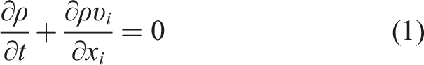
where
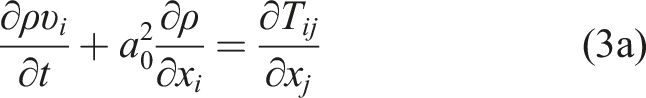
The momentum conservation equation is as follows:
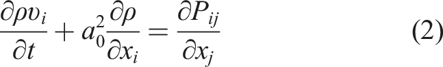
where

where
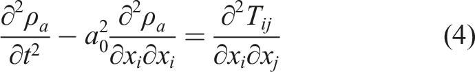
The above derivation shows that the Lighthill equation is the direct result of the mass conservation and momentum conservation equations and is, therefore, suitable for all practical flow problems, as well as the acoustic free jet emission challenge. However, it is difficult to solve since the nonlinear equation 3b contains a quantity
For the static fluid in an infinite region and a relatively small range of free turbulence without solid boundaries, the viscous stress inside the turbulence

Moreover, in isentropic conditions, the density fluctuation inside the free turbulence is exceedingly small, namely,

The aerodynamic noise calculation principle of rotating machinery
Actran/AeroAcoustics is based on the Lighthill method and combined with Curle’s theory: (1) The volume fraction of Curle’s equation is used as the volume source for the finite element region. (2) The area component of Curle’s equation is used as the boundary condition. (3) The Green’s function of the free field is employed for the other boundary conditions.
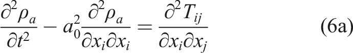
Curle’s theory is introduced based on Lighthill’s sound analogy theory. Equation 6a is integrated on the boundary
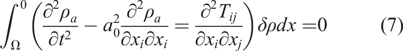
Integration by parts is used to produce weak variational form:
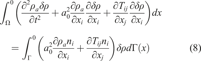
The stress tensor is used on the surface integral:
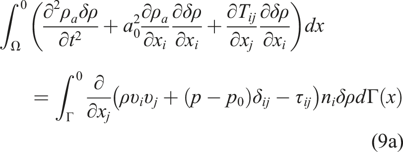

Equation 9a can be expressed as:
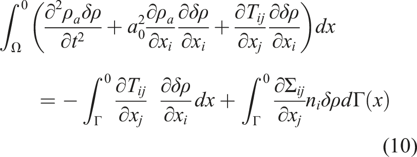
The first term on the right side of the equation represents the body source, while the second term denotes the surface source, corresponding to the noise of the rotating machinery. In the Actran software, it corresponds to the Lighthill body source and Lighthill surface source, respectively.
The numerical calculation of the flow-induced pump noise
The centrifugal pump noise spectrum displays broadband characteristics, with peaks ranging from tens of hertz to thousands of hertz (Liu et al., 2016). The peak value of the axial frequency and its higher harmonics in the spectrum is mainly caused by pressure pulsation, while the high-frequency off-peak noise primarily results from random noise, such as bubbles, turbulence, and shock. Therefore, this paper investigated (a) the vibrational noise caused by water pulsating pressure in the pump and (b) the vibrational noise caused after the turbulence generated by the water body in the pump is converted into a sound source. The specific steps were as follows: (1) Using the Fluent Mesh software, a CFD model was established to simulate water in the pump, including geometric cleaning, CFD mesh generation, and processing. (2) The steady-state debugging and calculation of the water CFD model were performed. The steady-state flow field information was provided, the time-averaged flow field was obtained, and the distribution characteristics of the velocity, pressure, and streamline in the pump were determined using the Fluent software. (3) The unsteady-state debugging and calculation of the CFD model in the pump were performed. The transient characteristics were analyzed, the periodic flow field characteristics of water movement in the pump were reproduced, the pulsating pressure at key points was detected, and the transient data for the flow-induced aerodynamic noise analysis were provided using the Fluent software. (4) Based on the results of flow field analysis, the acoustic calculation domain for flow-induced noise calculation was selected for acoustic grid division and processing. The acoustic model boundaries, components, and solvers were established for calculation using HyperMesh and Actran. (6) Seven blades were used at a rotational speed of 3,000 RPM, while the noise mainly occurred at the fundamental frequency and frequency multiplication of the water pump, that is, around 350 Hz and 700 Hz. The noise calculation typically needed to cover three times the fundamental frequency, that is, about 1,000 Hz. To capture more detailed broadband acoustic information, 2,000 Hz was selected as the highest calculation frequency. (7) The following sound source loading method was used to calculate the flow-induced noise: CFD transient calculation results were imported into the acoustic calculation software and converted into surface and volume sound sources, which were mapped to the acoustical grid using an integral interpolation method. The time-domain data were transformed into frequency-domain data via fast Fourier transform (FFT), after which the distribution characteristics of the noise sources were analyzed. (8) A sound propagation model was established, after which a nephogram of the sound pressure level distribution of the water in the pump was created, which was subjected to debugging and calculation. The sound propagation was determined, the distribution characteristics of the sound pressure were analyzed, and the sound pressure value at the monitoring point was obtained. (9) The fluid-induced noise calculation considered the fluid–solid coupling and pump vibration. Different operating conditions were established to determine the pump vibration characteristics caused by the various pressure components using Actran.
A flow chart of the flow-induced noise calculation is shown in Figure 1. Flow-induced noise calculation process.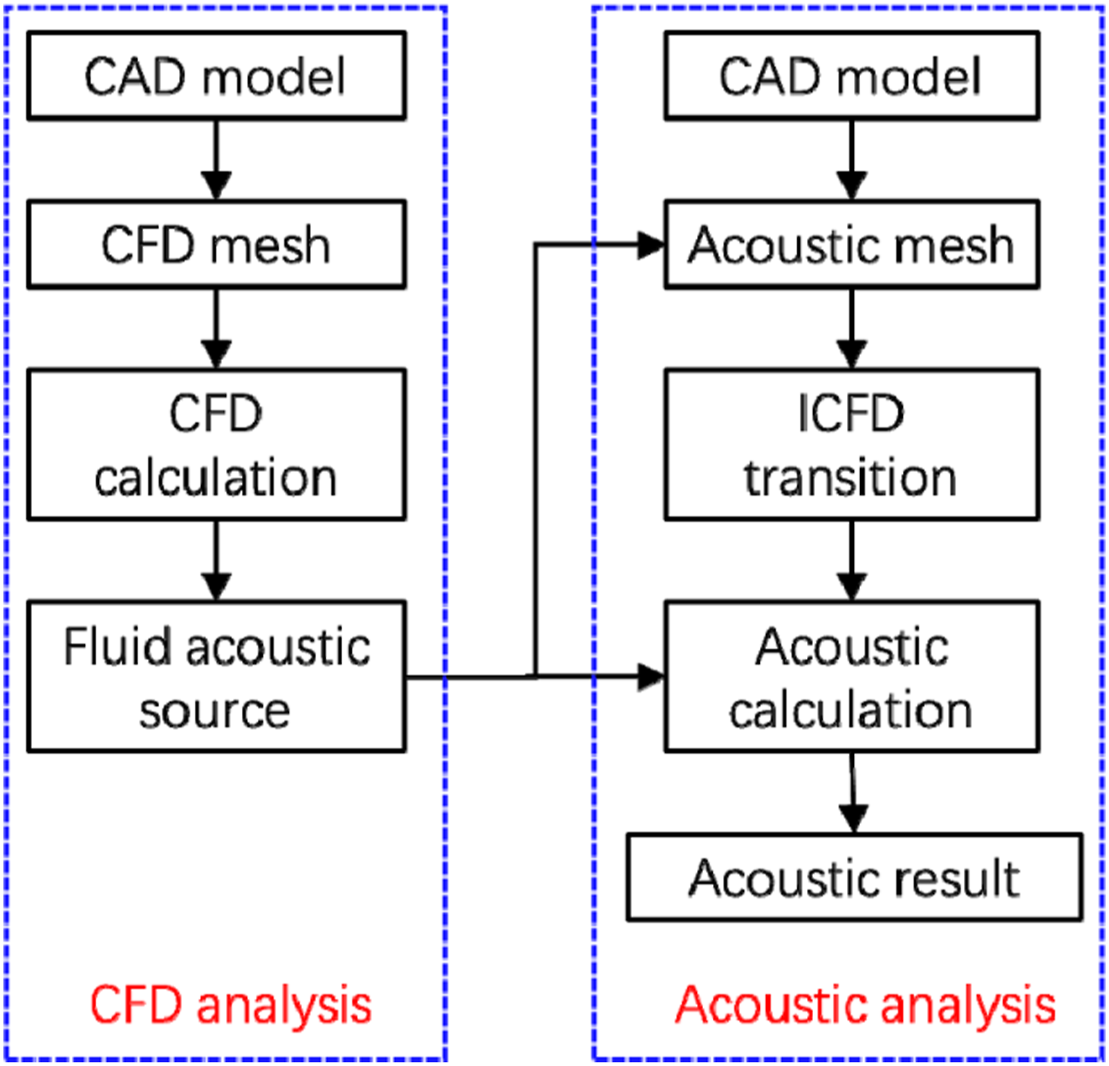
Fluid pressure pulsation and flow characteristics of centrifugal pumps
Geometric processing, meshing, and parameter establishment
The fluid domain of the pump model is shown in Figure 2. The fluid entered from the left, converting mechanical energy into kinetic energy via the rotational motion of the impeller, after which the downstream volute further converted kinetic energy into potential energy. A pressure difference was evident between the upstream inlet and the downstream volute of the impeller. The flow in the volute affected by the pressure difference returned to the inlet area via the clearance. Fluid domain of the pump model.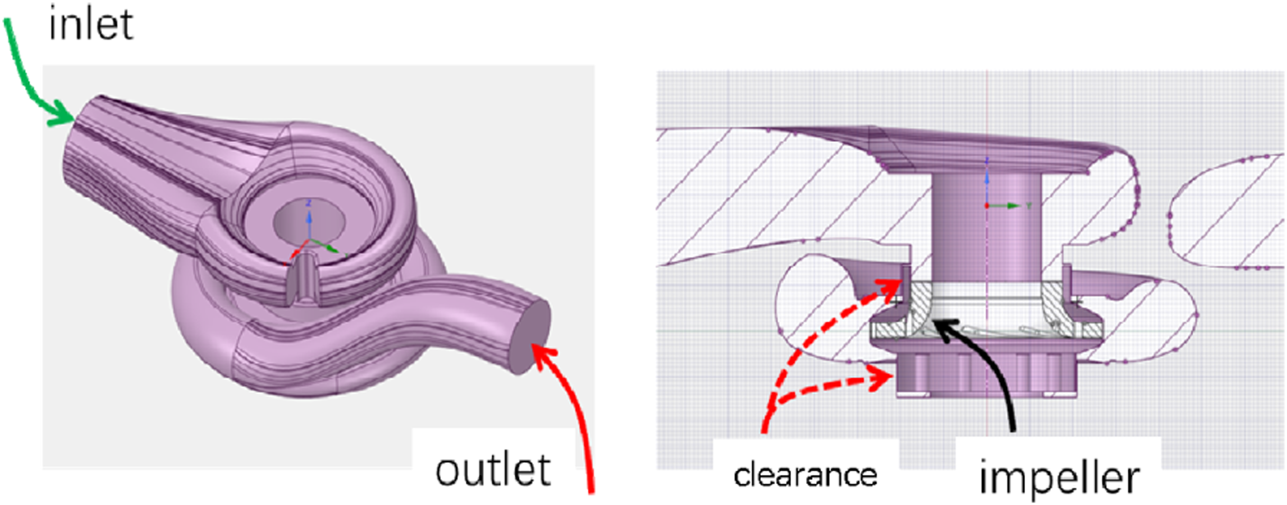
Since the upstream and downstream of the pump related to the pipeline during water pump operations, the inlet and outlet of the current pump were extended three to five times the diameter of the pipeline. The model was simplified using the ANSYS pre-processing software SpaceClaim, while the CFD grid was divided via Fluent meshing. The geometric models of the different parts were imported successively, and the corresponding grid sizes, curvature captures, clearance captures, and grid growth rates were established.
The corresponding parameters for the CFD calculation process were set using Fluent software, which included the physical parameters and boundary conditions, steady-state calculation process, and transient calculation process. The turbulence model and physical parameters are set as follows: (1) Set the model unit to millimeters based on actual dimensions. (2) Set up a turbulence model. In the flow calculation of the water pump impeller, the flow is in turbulence, and the industry commonly uses the RNG turbulence model; this model can better capture the flow field of rotating flow, and wall functions are used at the wall, with non-equilibrium wall functions commonly used in the industry. (3) Add water properties parameters. The viscosity parameter of water density is set to the default value.
The boundary conditions were established as follows:
The rotational speed and direction were determined according to actual conditions. In this case, the flow direction of the impeller was in the Z direction. The clockwise rotation was positive along the flow direction, while the counterclockwise rotation was negative. Therefore, the fan rotated positively. The rotational speed and direction were determined according to actual conditions at a relative rotational speed of 0 rad/s. The rotational speed was given because it was within the rotational region. In this coordinate system, the blades were relatively stationary. The inlet speed was calculated based on the operational flow rate and inlet area of the water pump equipped with a pressure outlet. The inlet and outlet turbulence intensity was established according to that of a uniform atmospheric environment at about 5%, with a turbulent viscosity rate of 10.
The turbulence model, recognized as more accurate in the industry, was used for separated vortex DES simulation to capture the large and small eddies generated by the rotation of the impeller. To distinguish the computing regions more accurately, the DDES model is recommended. The time term used a second-order implicit scheme, while the momentum equation used a boundary center difference scheme. Several vital parameter determination principles were used to initiate the transient calculations.
The determination of the time step was related to the frequency of the calculation required. The time step for the simulation calculation was generally considered the time interval when the blade rotated by 1–3°. In this case, the time required for the blade to rotate by 3° was Δ T=(3*60)/(360*3000) = 0.00016667s, while the maximum frequency corresponding to this time step was 3,300 Hz, which can meet the frequency range that the water pump is concerned about.
For each iteration within a time step, it was necessary to ensure that the time step converged. The judgment could be based on whether it was reduced by an order of magnitude from the beginning to the end or monitoring a physical quantity that remained unchanged when the physical iteration reached a certain number of steps. In this case, 15 iterations were judged to ensure the convergence of the time step, and 15 iterations were selected.
The determination principle of the time step: the flow field that obtained quasi-periodic signals was determined based on the pressure fluctuation at the monitoring point.
The geometric model above was imported into the Fluent messaging software, and the mesh size, curvature capture, clearance capture, and mesh growth rate were established, as shown in Figure 3(a). The maximum value of the grid was derived from the frequency of the subsequent aero-acoustic calculations. The maximum frequency was 4,000 Hz, while the corresponding wavelength was 85 mm. The maximum grid value was set as 10 mm according to an eight-grid division per wavelength. After importation, the Fluent mesh automatically converted the geometry to face meshes. Figure 3(b) shows an enlarged display of the local surface grid of the inlet interface. Inlet grid division diagram.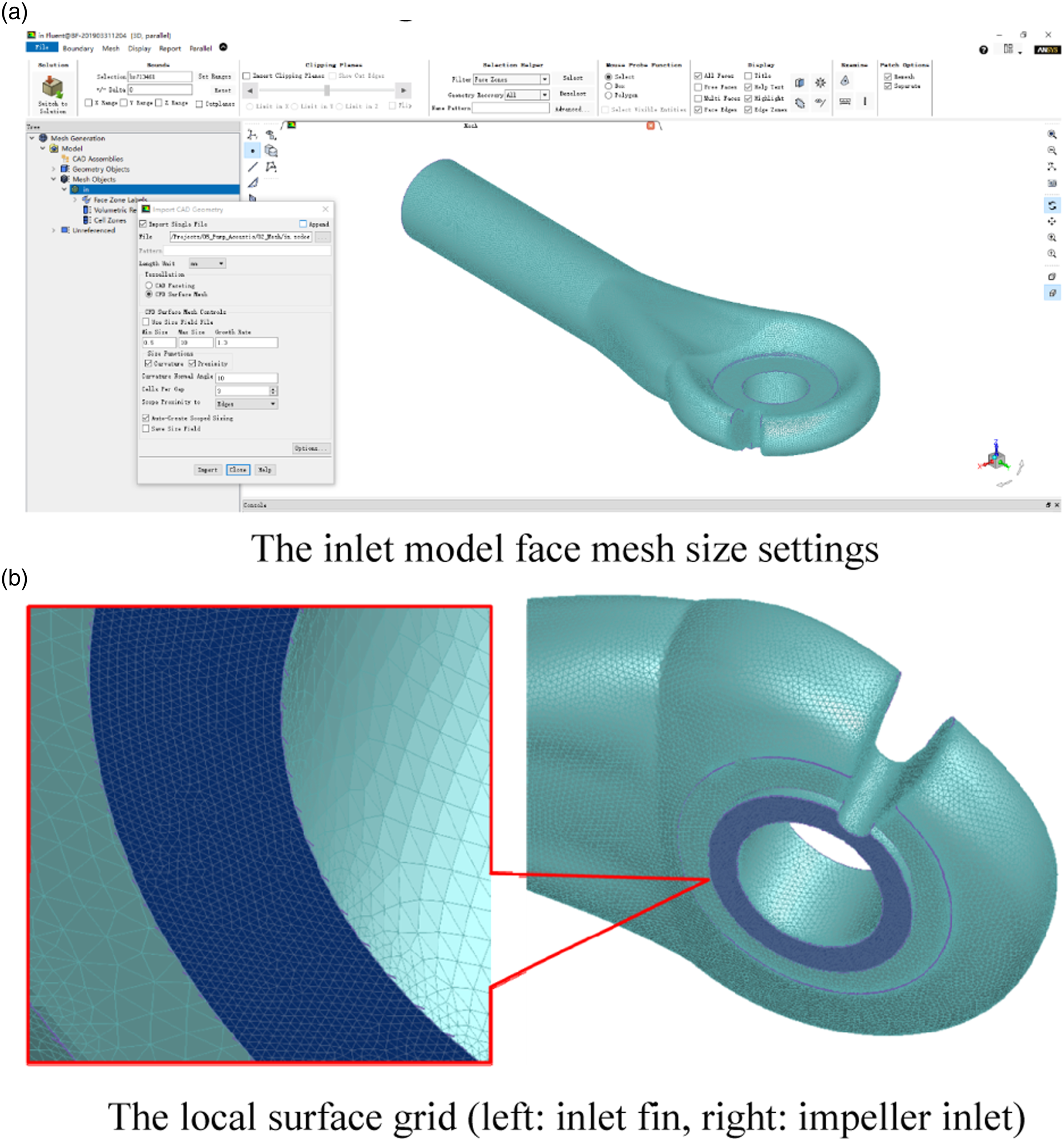
The import grid generation process allowed an export area grid to be generated, as shown in Figure 4. Exit grid division.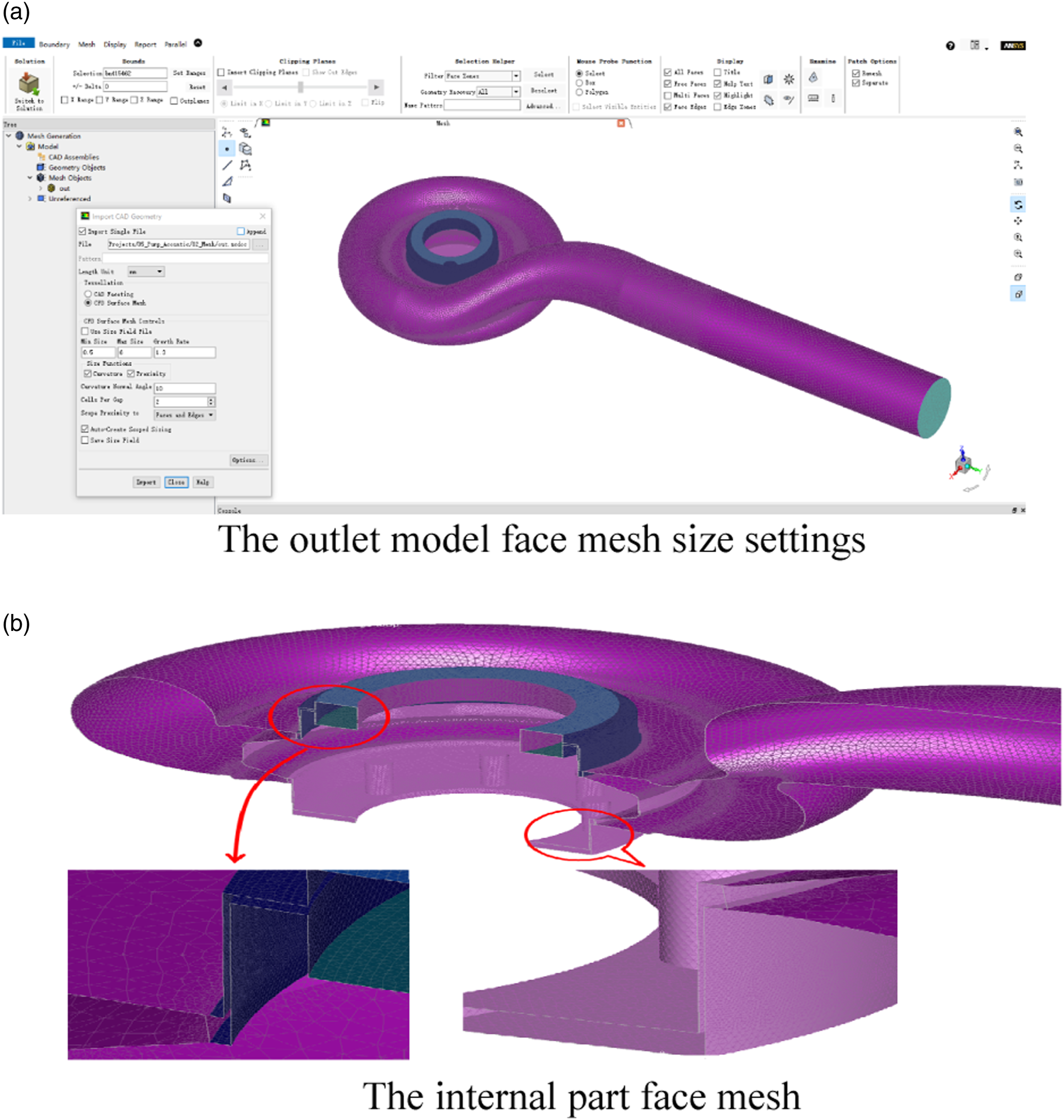
Since the impeller produced significant noise due to high-speed rotation, it was necessary to divide it into a denser grid. The impeller grid division settings are shown in Figure 5. Impeller grid division.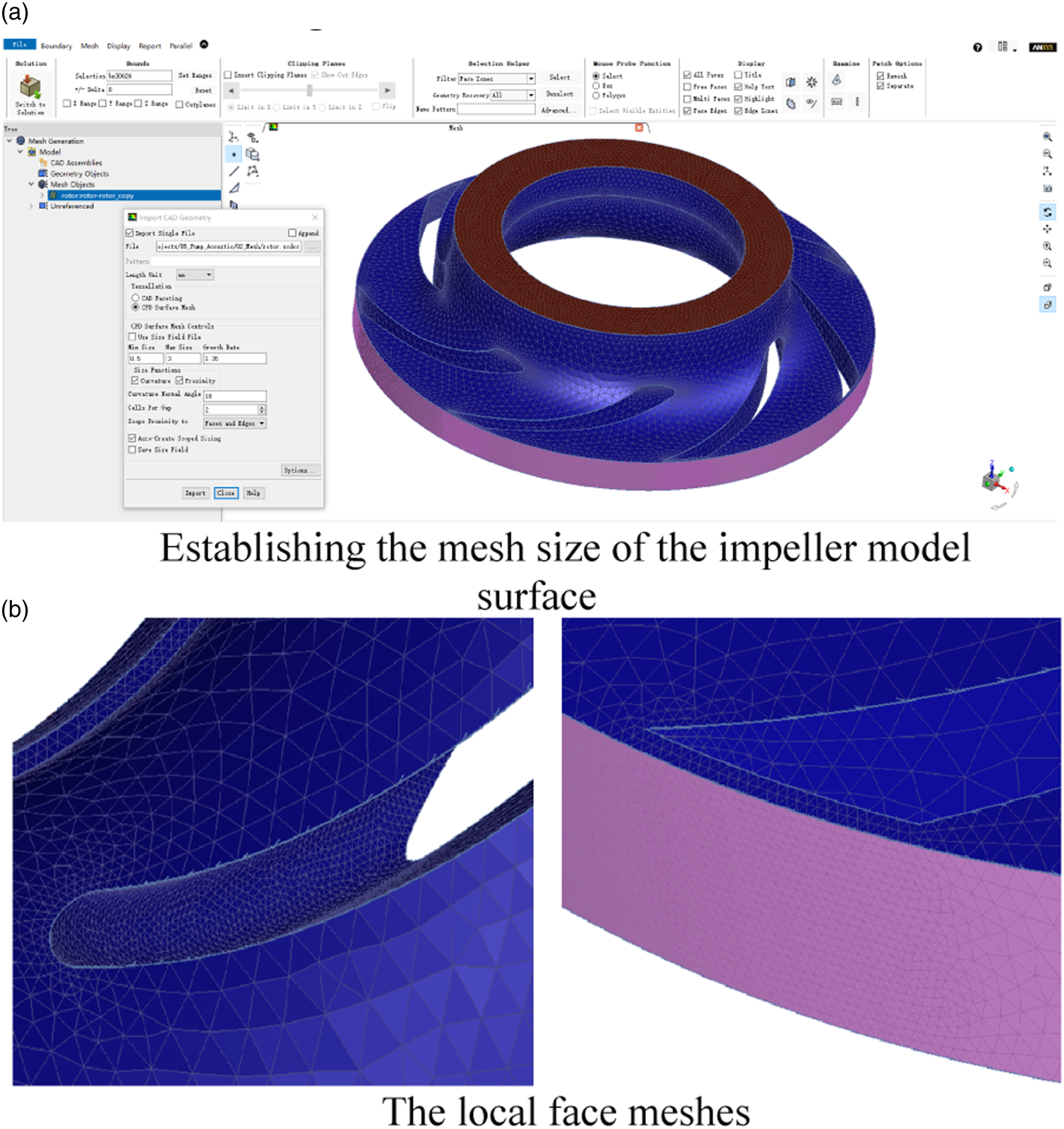
The meshing of the different parts was followed by mesh assembly and volume meshing using the software. The inlet, impeller, and outlet grids shown above were selected and imported into Fluent messaging. The merged model and grid file are shown in Figure 6(a). The single-connected region in the assembled model represented a fluid domain and was denoted by the inlet, impeller, and outlet regions. Corresponding quality points were established for these single-connected regions, as shown in Figure 6(b). The mesh was named, and the boundary attribute settings were established. Fluent messaging was used to name boundaries quickly and efficiently within the manage face zone and establish boundary conditions, such as entrances, exits, interfaces, and walls, as shown in Figure 6(c). Meshing of the different parts.
After completing the steps above, a volume mesh was generated, as shown in Figure 7(a). The vertical section of the water pump and the partially enlarged clearance volume grid are shown in Figures 7(b) and (c). Grid of the different parts.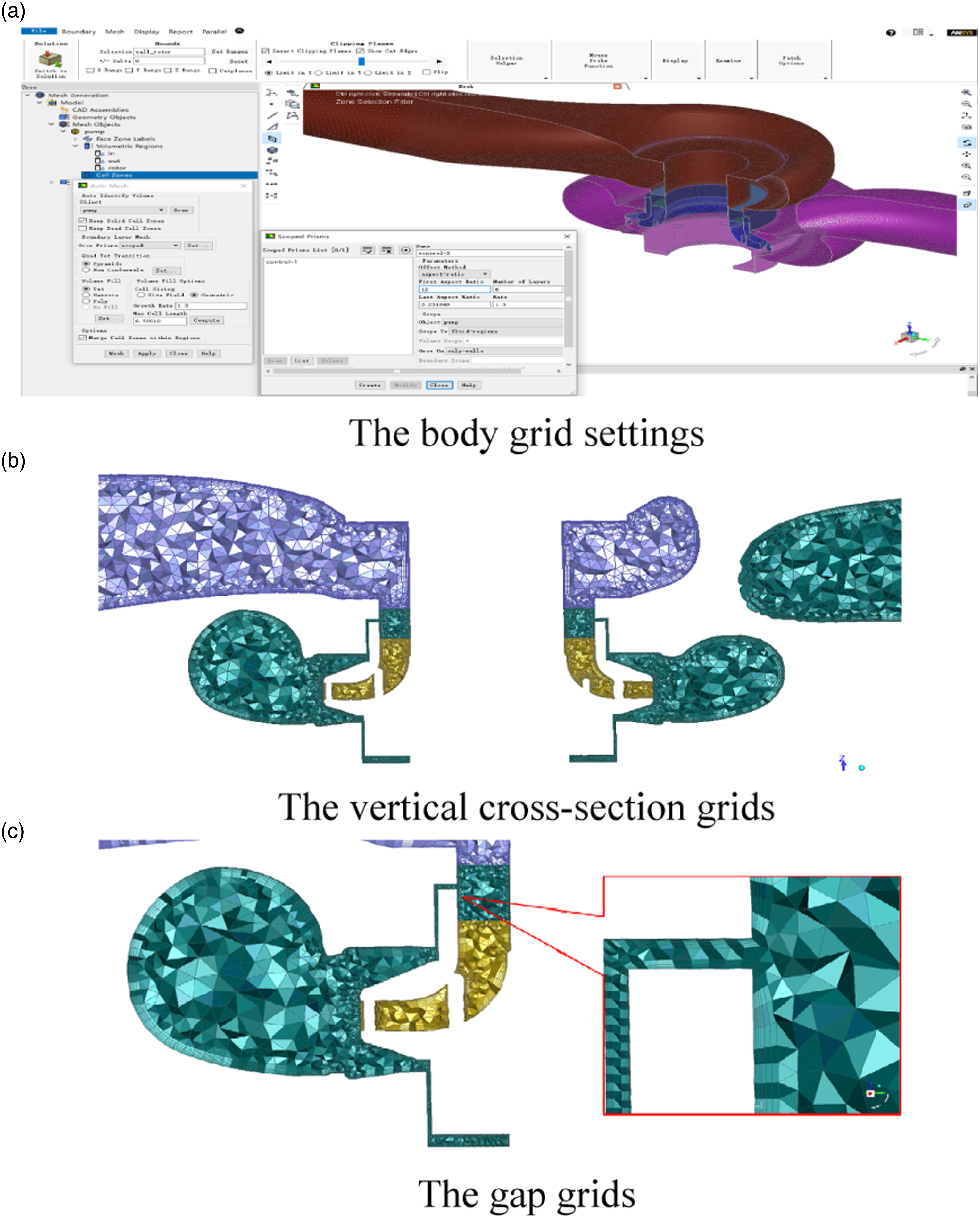
Analysis of the calculation results of the water flow field in the pump
Figure 8 shows the flow line distribution in the pump. The flow line distribution in the entire space was smooth, with no significant flow separation since the vortex tongue displayed bias in the axial direction to avoid the direct collision of high-speed fluid at the impeller outlet. A comparison between the two clearance sizes showed no comparatively large effect on the internal flow of the water pump. Comparison between the internal flow lines of the water pump.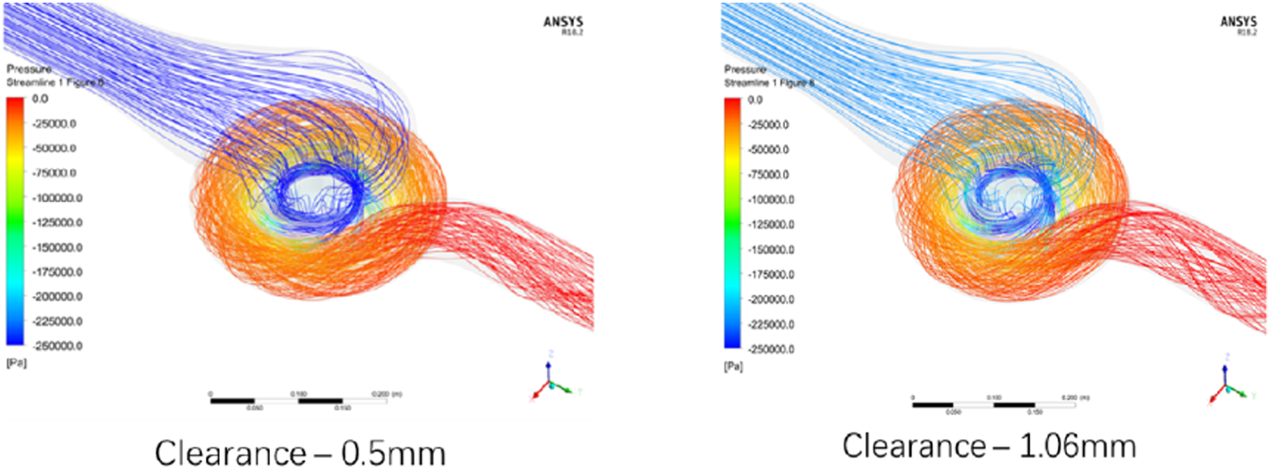
The comparison between the flow lines in the upper clearance is shown in Figure 9(a). The velocity of the 0.5 mm clearance was below 15 m/s, decreasing gradually within the clearance. When the clearance was increased to 1.06 mm, the internal flow velocity exceeded 15 m/s, showing no significant decline within the clearance. The comparison showed that the annular component of the 0.5 mm clearance outlet velocity was not comparatively large. However, the annular velocity of the 1.06 mm clearance outlet was high, increasing the inlet flow pre-rotation at the downstream impeller inlet, resulting in the angle-of-attack loss at the leading edge of the blade. The flow line distribution of the bottom clearance is shown in Figure 9(b). The fluid velocity in the clearance was low, while the influence of different clearance sizes on the flow in the volute was not comparatively large. Comparison between the flow lines in the clearances of the different parts.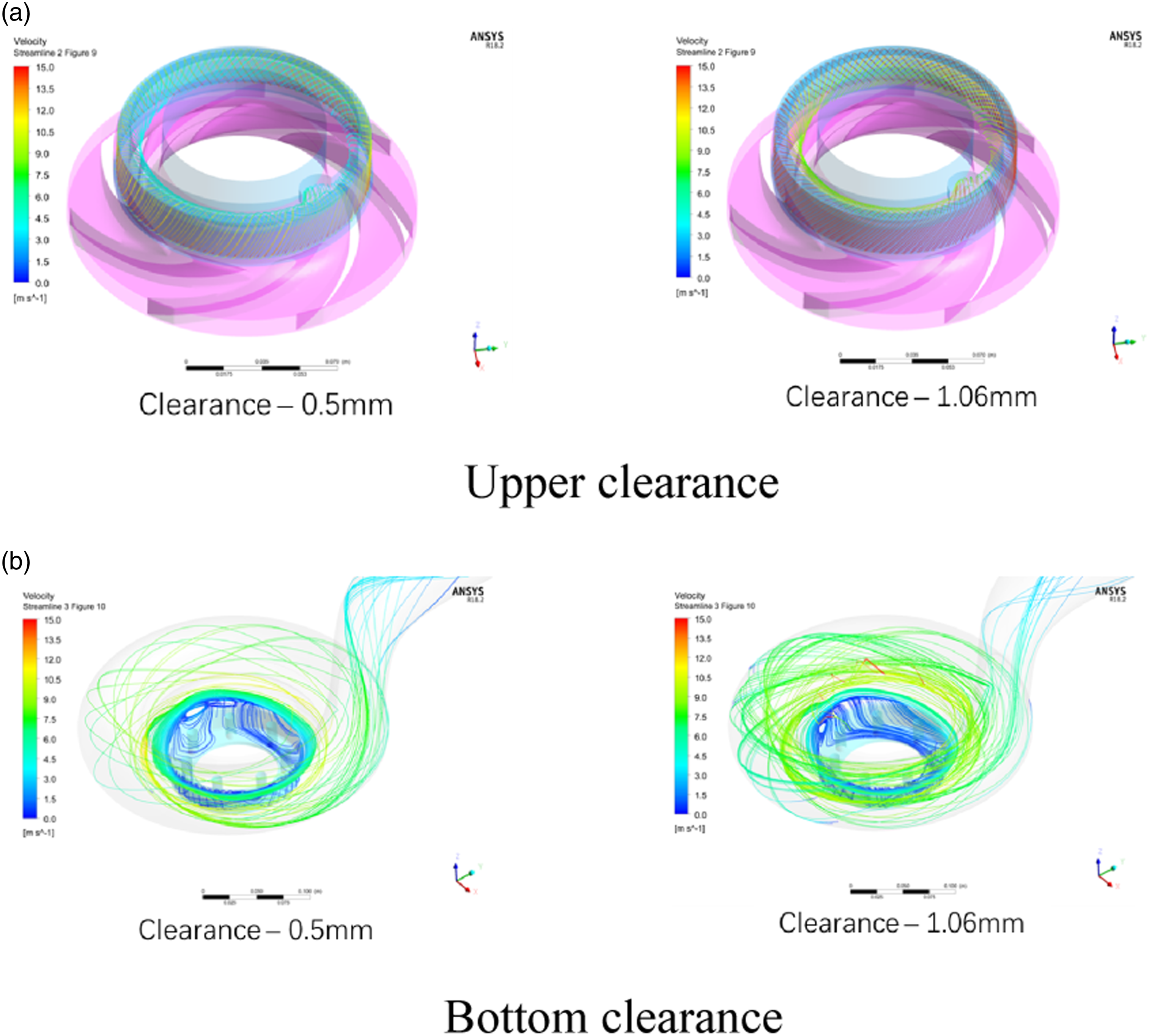
Figure 10(a) shows the pressure distribution on the surface of the pump volute. During the current simulation calculation, the relative pressure at the outlet was set to zero, while the relative pressure at the inlet was calculated according to the momentum conservation equation. The inlet pressure of the volute surface was the lowest. The high-speed rotating impeller converted the kinetic energy into potential energy in the volute, significantly increasing its surface pressure. Furthermore, the different clearances were compared. The pressure difference between the pump inlet and outlet decreased, corresponding to the 1.06 mm clearance, indicating that the clearance size significantly influenced the pump head. Figure 10(b) shows the pressure distribution at the pump cross-section. The velocity was increased by a flow area decline at the impeller. According to the Bernoulli equation, the static pressure was at the minimum value, while the pressure distribution in the volute was consistent with the radial position. A distinct pressure difference was evident since the upper seal was connected to the volute and impeller inlet. The lower seal was a closed area, displaying no significant pressure differences. Comparison between the pressure distribution in the different parts.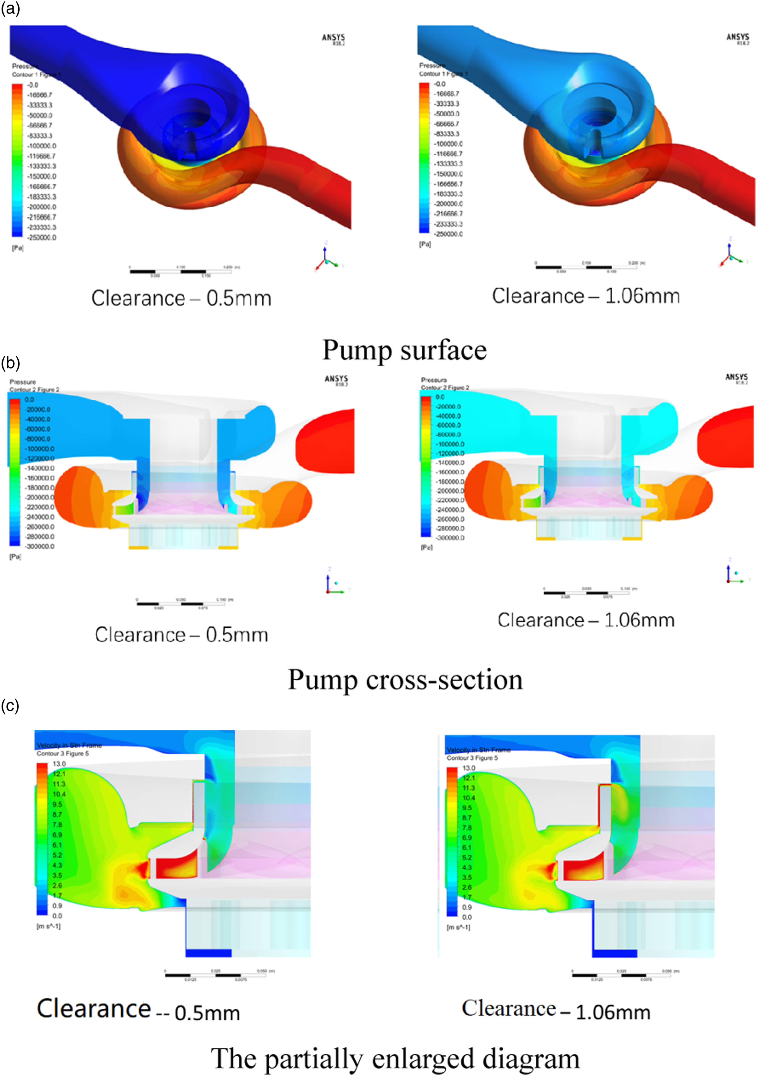
Figure 11(a) shows the velocity distribution of the pump section. The high-speed area in the current flow passage was mainly located near the radial outlet of the impeller and in the upper clearance. Since the lower seal clearance was a one-way closed structure, the speed is exceedingly low. The fluid velocity near the inlet of the impeller was 3–4 m/s and 6–10 m/s in the volute. Since the current velocity gradient in the spiral case was not significant, it might not generate substantial discrete noise. When the clearance increased from 0.5 mm to 1.06 mm, the velocity in the upper clearance was distinctly higher, with comparatively large disturbance in the upstream of the impeller. The relationship between the fluid velocity in the downstream clearance and the clearance size was not obvious. The distinct velocity separation at 90° in the current inlet area showed that the design modification could reduce the flow field disturbance. Figure 11(b) shows the influence of the upper clearance fluid on the fluid distribution upstream of the impeller. The clearance outlet was perpendicular to the direction of the incoming flow from the impeller, while the internal flow velocity exceeded that of the incoming flow. This resulted in comparatively large velocity separation in the local area, leading to turbulence intensity differences in the incoming flow of the impeller and more significant hydraulic loss and noise intensity. Comparison between the speed distribution in different clearances.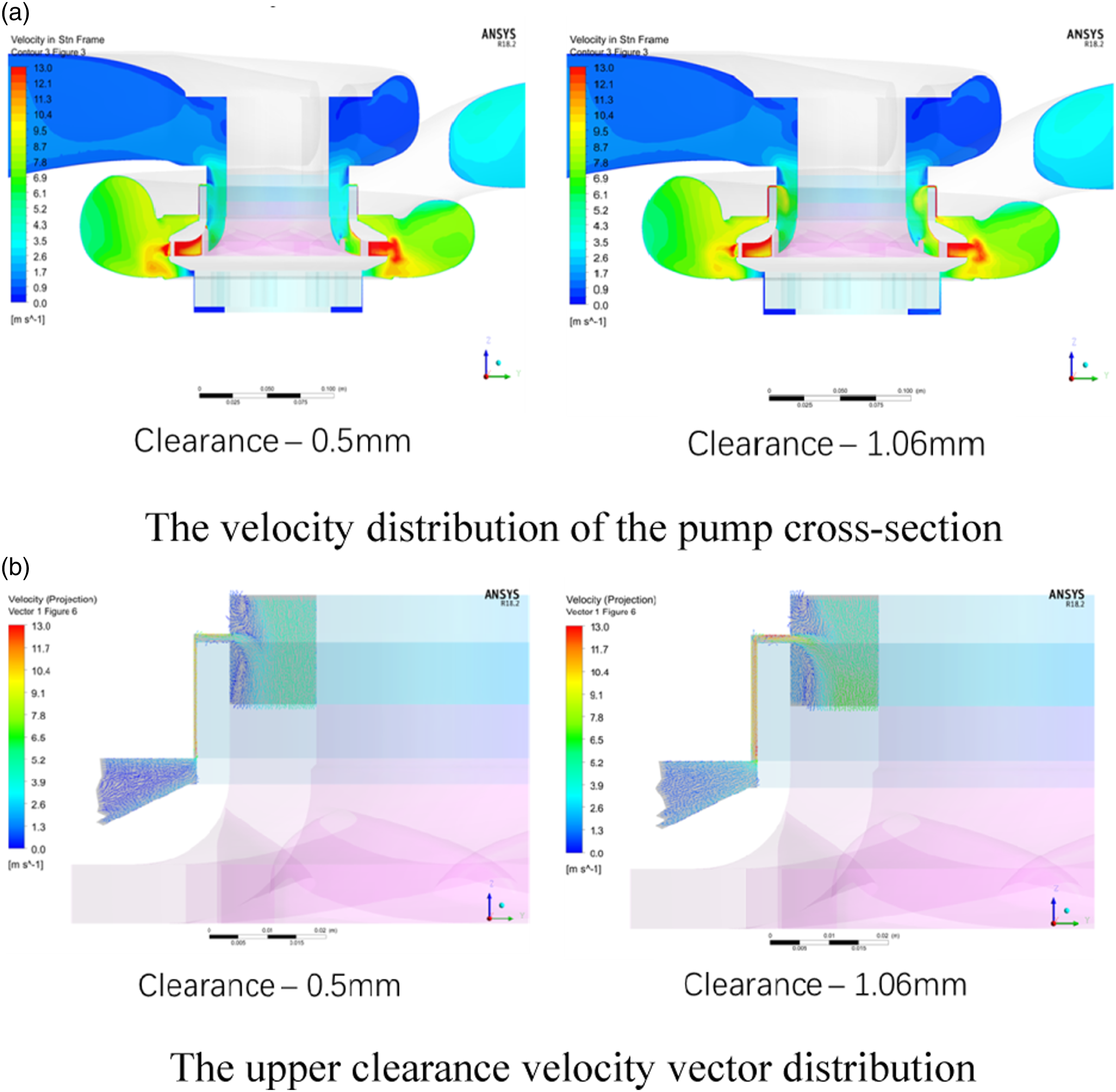
The vortex distribution generated by the upper clearance fluid in the incoming flow is shown in Figure 12. The vortex intensity generated by 0.5 mm clearance at the impeller outlet is significantly lower than that of 1.06 mm clearance. The larger mouth ring clearance may cause stronger structural vibration, and the interference between the incoming vortex and downstream blade may increase the intensity of middle- and high-frequency internal noise. Vortex distribution at the upper clearance outlet.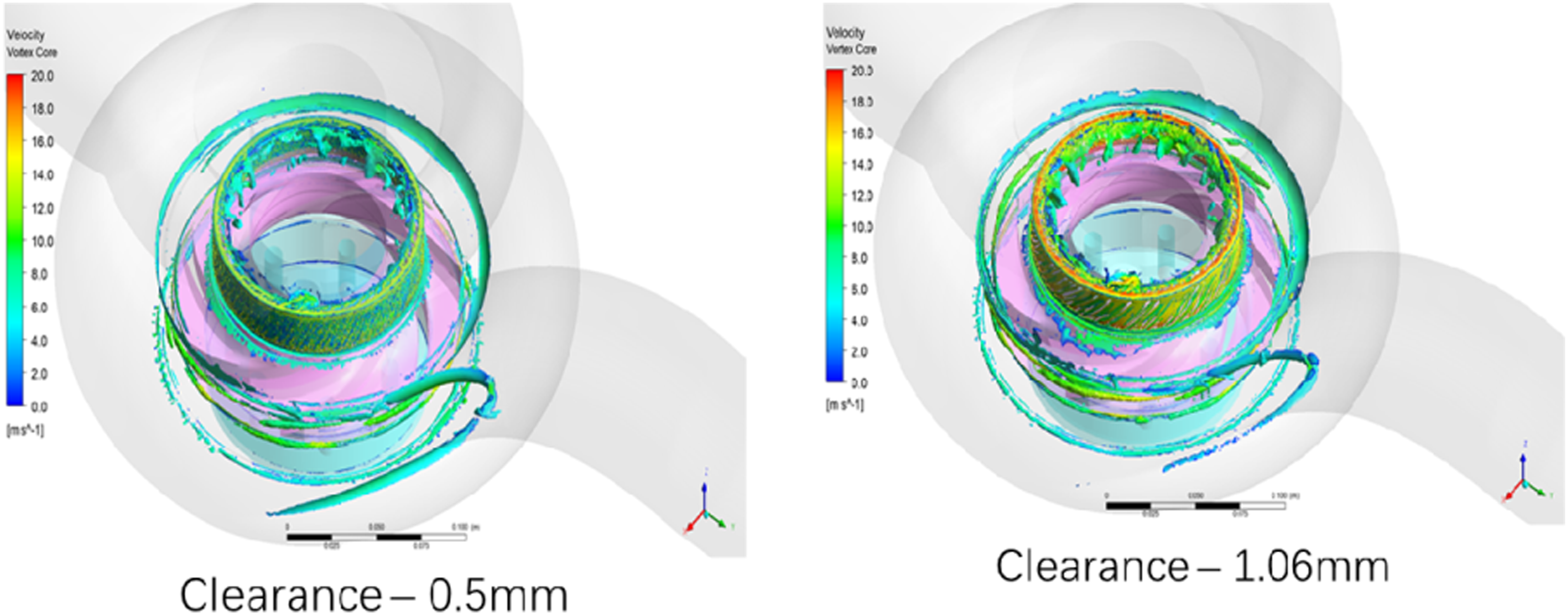
Flow-induced vibration and noise characteristics of the centrifugal pump
Geometric processing, meshing, and parameter establishment
Since the grid in the acoustic and vibration coupling calculation model only required six to eight mesh scales per wavelength, there was no need to establish a boundary layer or deliberately build hexahedral units, and the more convenient HyperMesh software was used for grid processing. The grid model in this paper is shown in Figure 13. The directivity monitoring point was selected 1 m from the pump casing surface. Acoustic calculation grid model.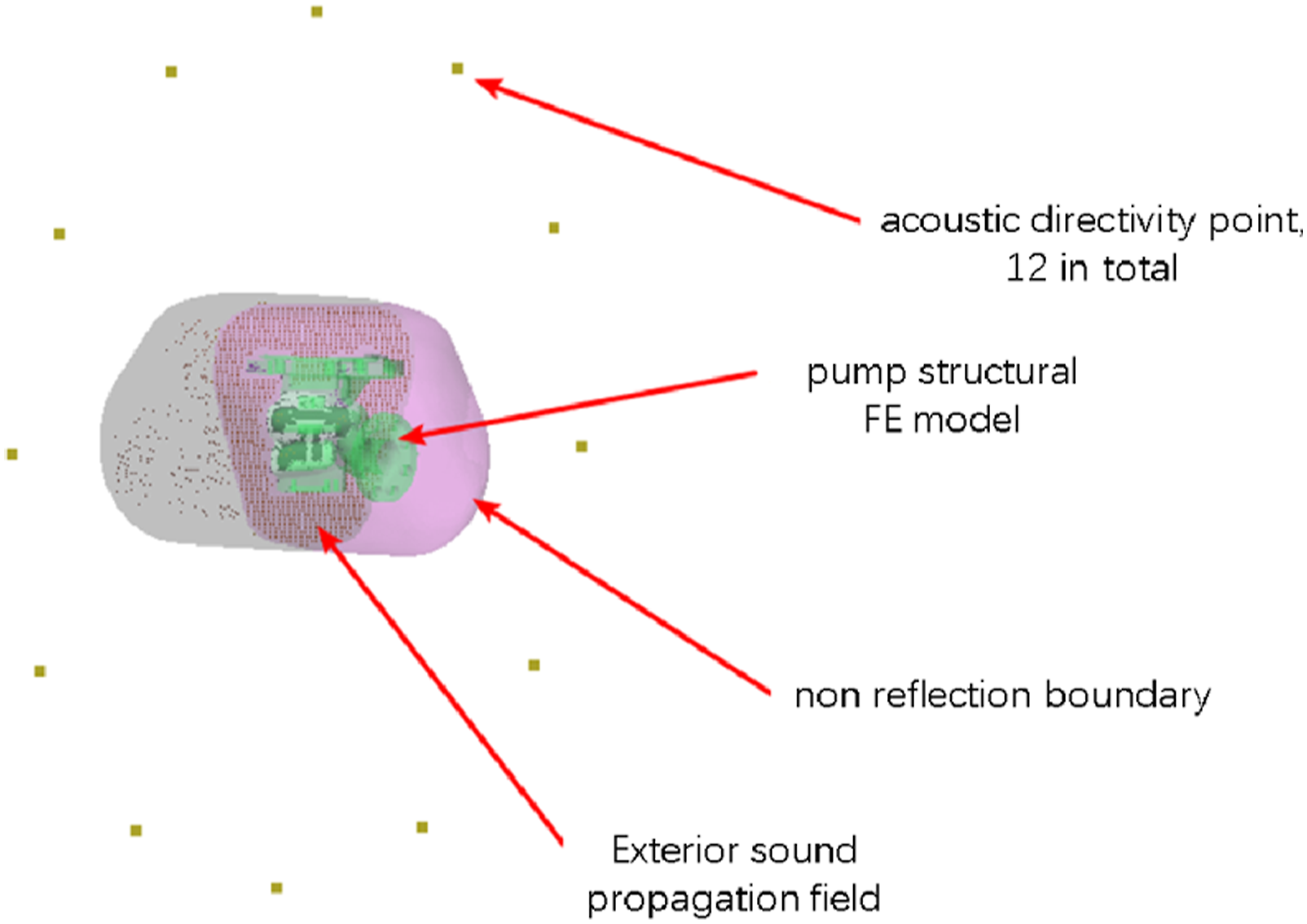
The vibration measurement points on the pump casing surface were set as follows: a total of six measurement points were selected, including four at the reinforcement bar located at the top of the pump casing and one at the back of the inlet and outlet pipe interface, respectively.
When processing CFD meshes, the pump impeller and the fluid domain between the impellers require refinement, while each detail must be established. Only the surface and body sound sources require extraction for rotating machinery. The surface sound source only needs to determine the interface surface mesh in CFD, while the internal details of the impeller region do not need to be established, as shown in Figure 14. CFD sound source loading surface.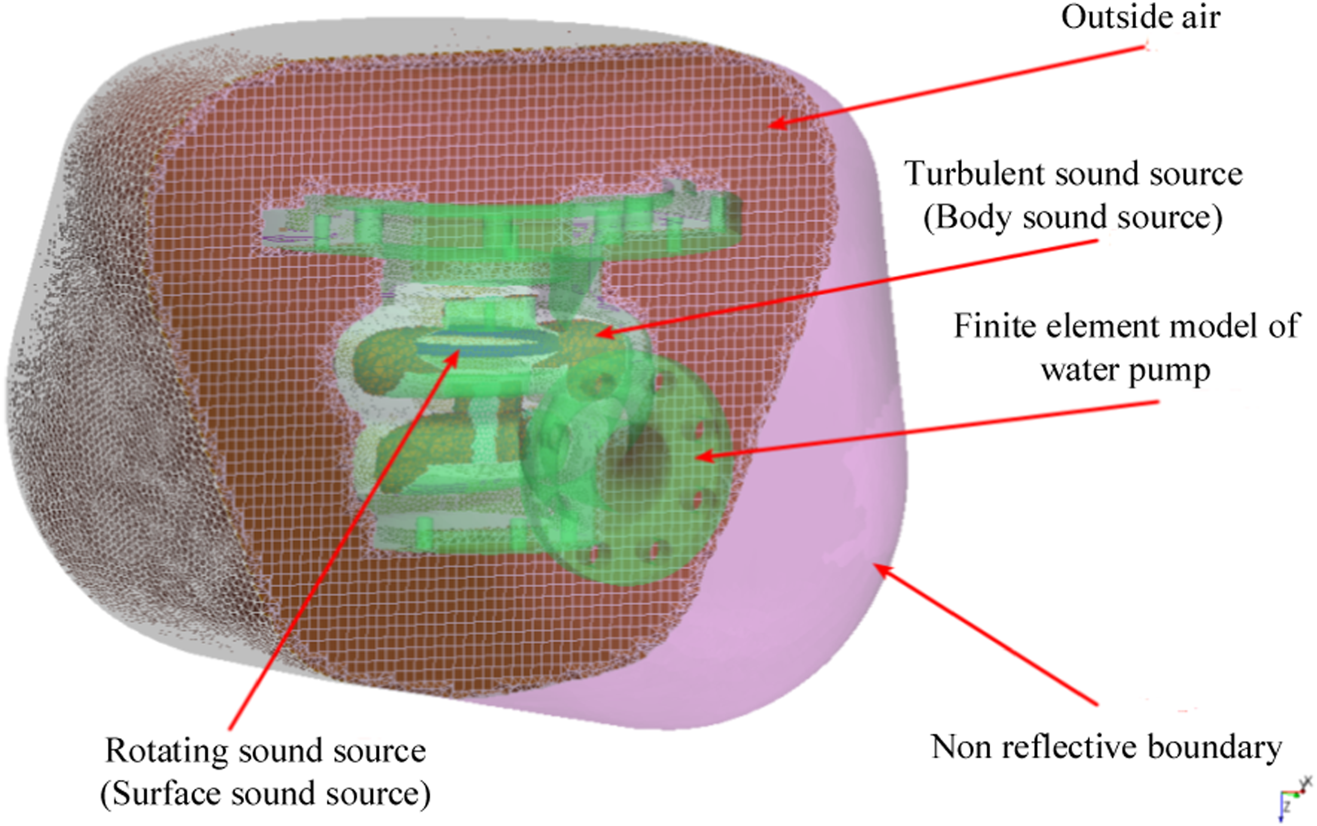
The boundary constraint form of the pump body in the acoustic calculation model was consistent with the actual installation and operational state, namely, three-sided elastic installation. Therefore, the constrained parts in the acoustic simulation calculation model were at the top of the pump casing and the inner surface of the bolt hole of the inlet and outlet pipes. The constrained freedom was represented by the axial translational freedom of the three pipeline sections, while the remaining translational and rotational freedom was released. The pump casing boundary constraint diagram is shown in Figure 15. Boundary constraints of the pump casing structure.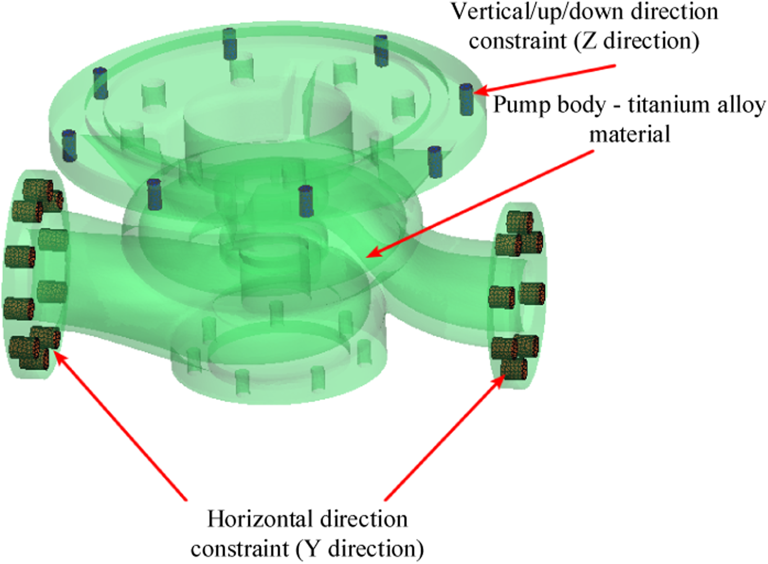
The pump body design drawing identified the pump casing material trademark as ZTA1, referring to titanium alloy. Its material properties related to acoustic calculation included a material density of 4500 kg/m3, an elastic modulus of 1.18 × 10¹¹ Pa, and Poisson’s ratio of 0.34.
The calculation model included both an acoustic propagation area grid and a pump structure grid. Figure 16 shows the sound propagation area inside the pump body and structural grid. Pipeline modes were established at the inlet and outlet of the sound propagation water area inside the pump body to simulate the non-reflective boundary conditions of fluid entering this region. Acoustic transmission area inside the pump body and structural grid of the pump casing.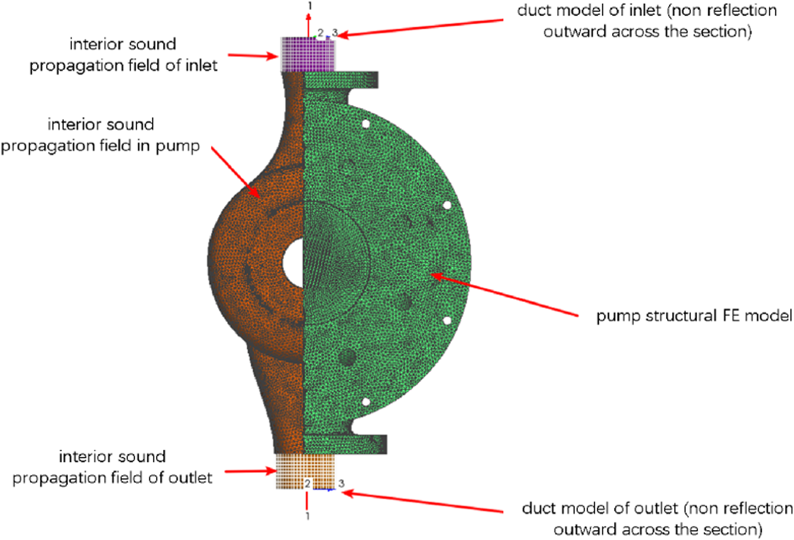
Analysis of the pump body vibration and noise calculation results
Figure 17 shows the sound source distribution results of the fluid-induced vibration and noise calculation in three water pump sections. Sound source distribution results of the flow-induced vibration noise calculation in three water pump sections.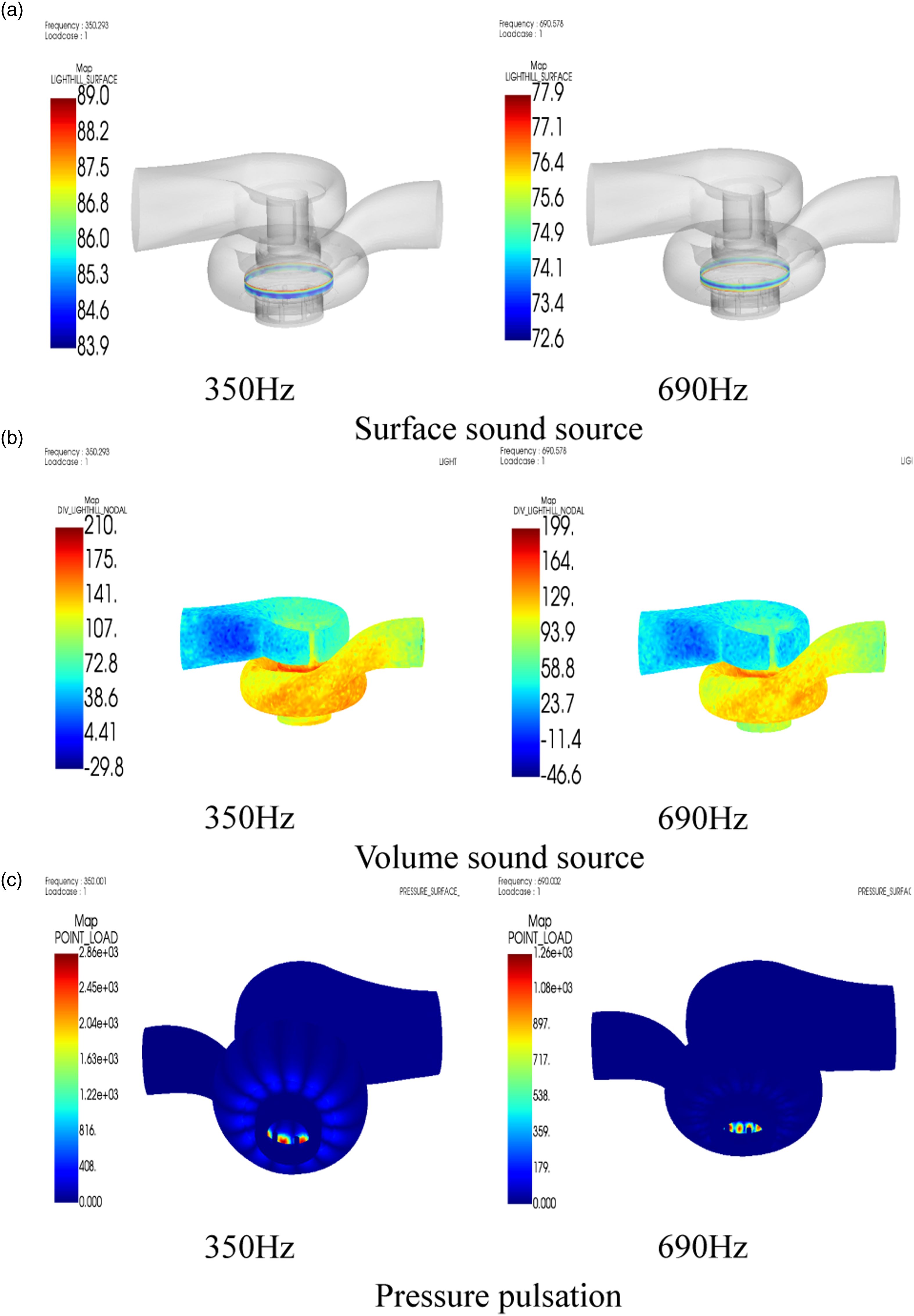
Before and after changing the mouth ring clearance, the dimensions were 0.5 mm and 1.06 mm, respectively. The weighted acceleration values of each measuring point on the water pump casing at two mouth ring clearance dimensions are shown in Figure 18. The main peak frequency of the acceleration on the pump casing surface was around 700 Hz, which was twice the blade frequency. Furthermore, due to the fluid turbulence, a high-frequency band of 1,800–2,000 Hz excited a larger acceleration response value. When the mouth ring clearance increased, the peak vibrational acceleration value of each measuring point on the pump casing surface was distinctly higher than the vibrational response of the structure at the original mouth ring clearance size. Weighted acceleration curves of the different water pump measuring points.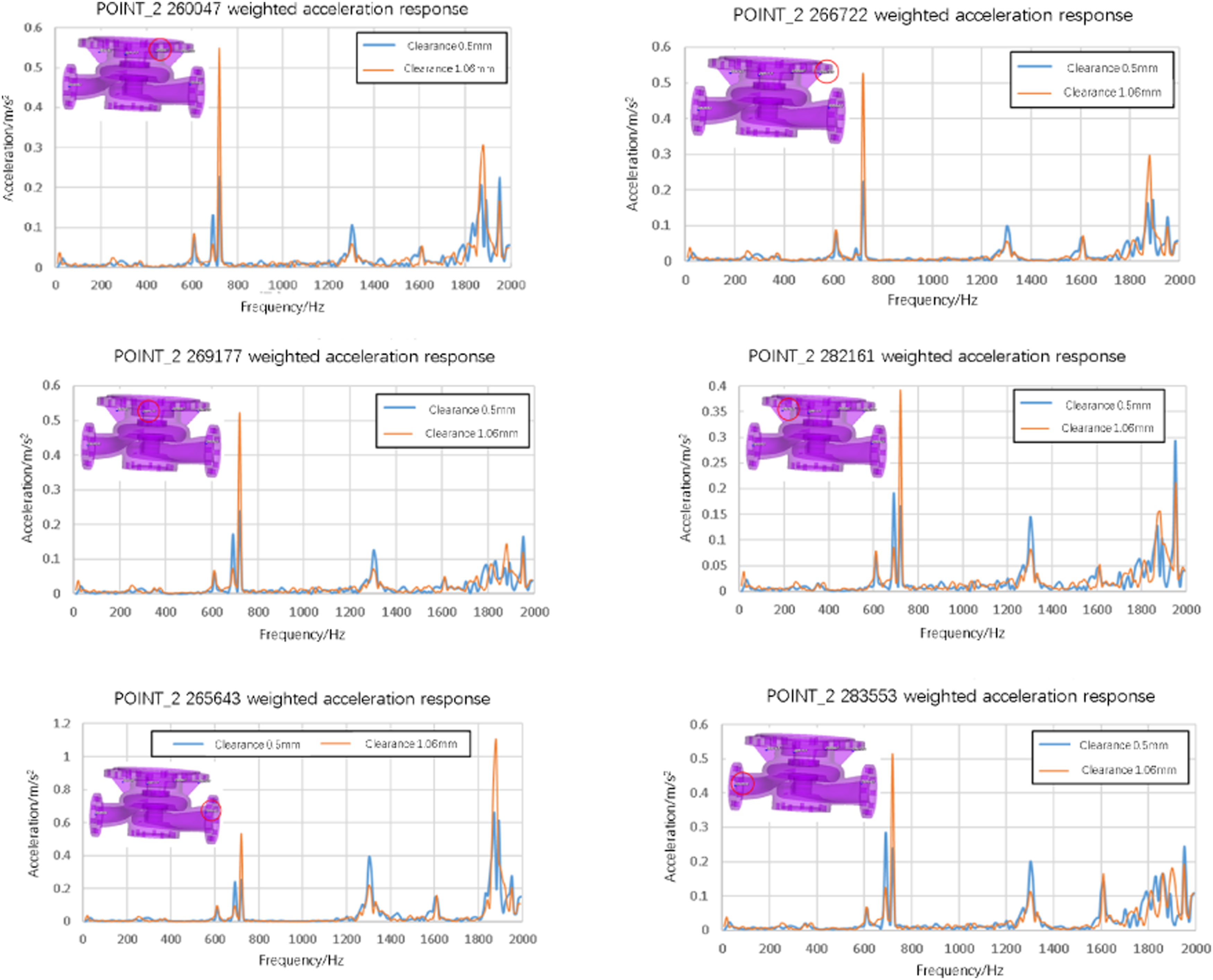
Figure 19 shows the nephograms of the displacement responses at the blade frequency and twice the blade frequency on the pump casing surface (350 Hz and 690 Hz, respectively) at a mouth ring clearance of 0.5 mm. The displacement response at twice the blade frequency exceeded that at the blade frequency, which was consistent with the acceleration frequency response curve results at the above measuring points. Displacement nephogram at the leaf frequency.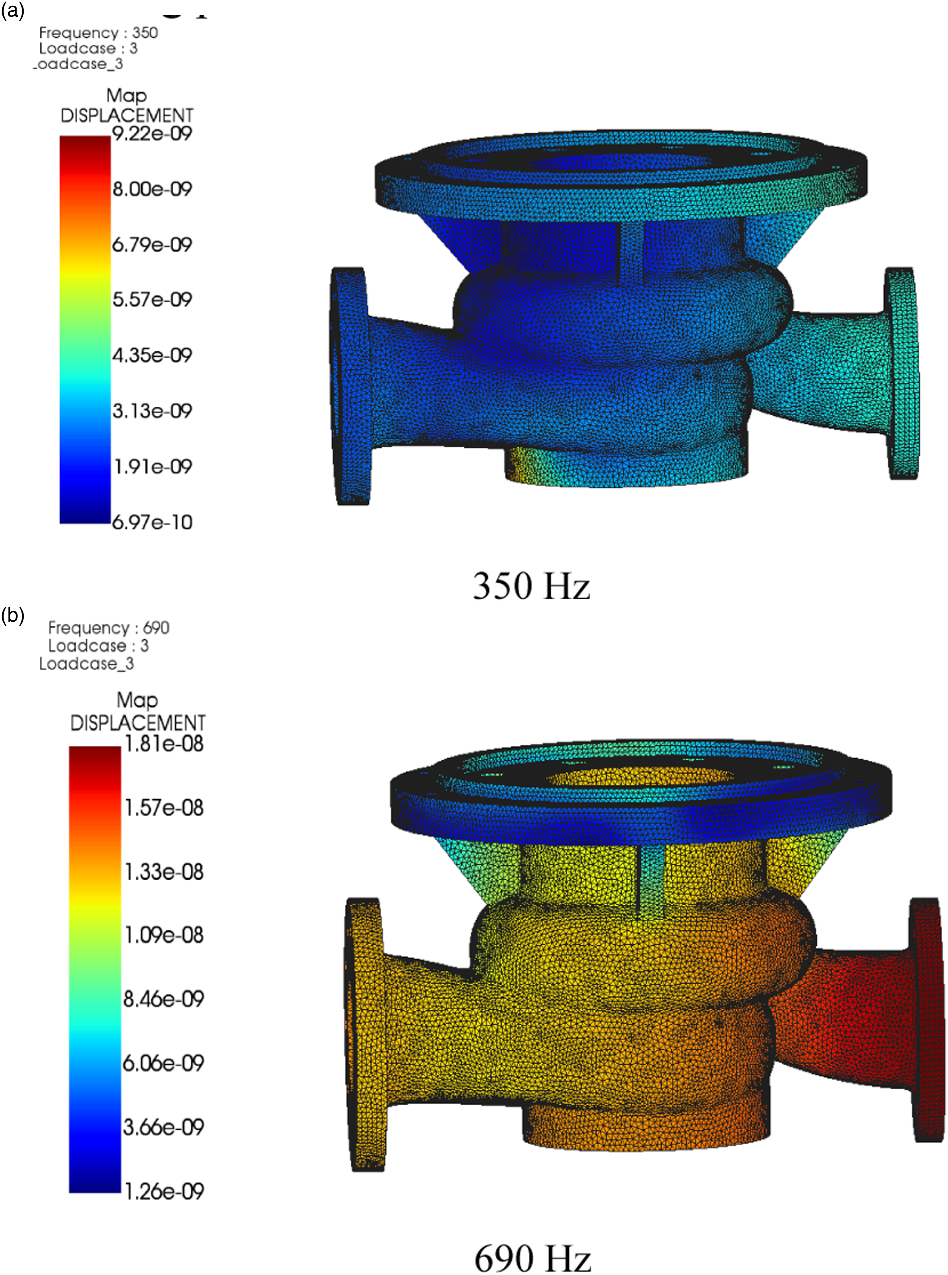
Figure 20 shows the sound pressure frequency response curve comparison before and after changing the mouth ring clearance at the external sound field measurement point, 830952. When the clearance of the mouth ring increased, the sound pressure level at twice the blade frequency (690 Hz) changed slightly. However, the overall sound pressure level in the entire frequency band displayed no changes, that is, the mouth ring clearance modifications minimally affected the external sound field change. The response level of the sound pressure outside the pump casing was mainly caused by fluid pulsation pressure. The sound pressure level at each frequency point exceeded that is caused by the fluid turbulence sound source. Comparison chart of the sound pressure level curve of the 830952-measuring point after enlarging the annular clearance.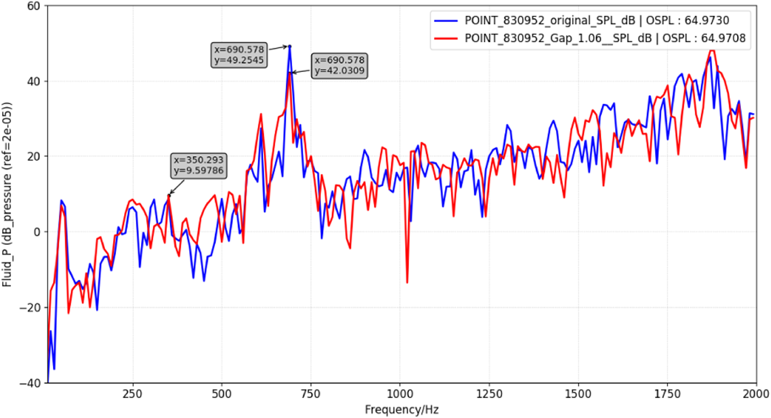
Figure 21 shows the sound pressure level response nephogram of the external sound field of the pump casing at the blade frequency and at twice the blade frequency. The nephogram can be used to observe the sound pressure level distribution of the external sound field at each frequency. The response value of the external sound field pressure level was higher at 690 Hz than at 350 Hz. Cloud chart of the sound pressure level response in the external sound field.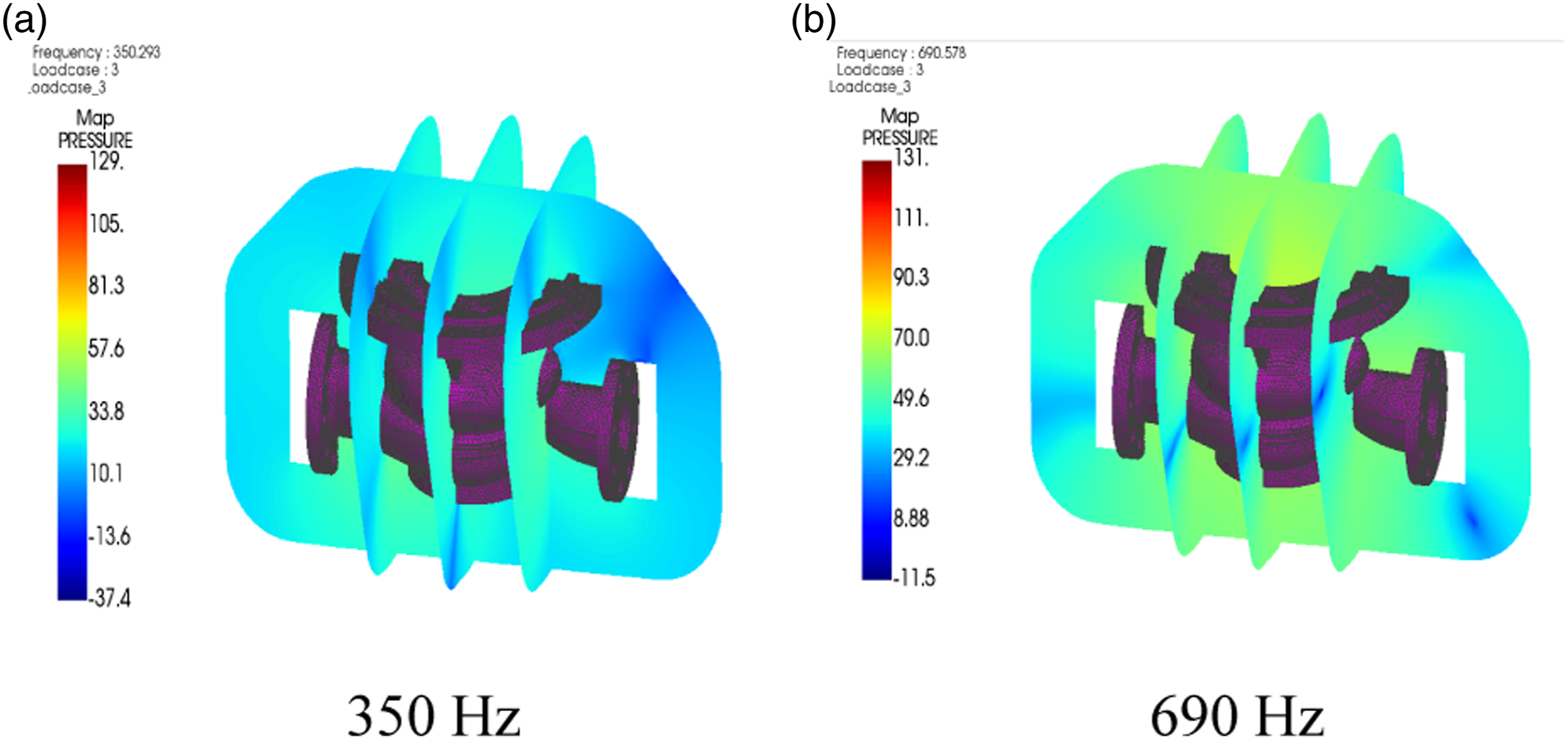
Conclusion
This paper examines the impact of flow-induced vibration noise and structural parameter changes on the sound field of marine centrifugal pumps. Pump models are subjected to pre-processing, calculation, and CFD analysis, while the flow-induced vibration noise in the pumps is determined and assessed. Acoustic simulation is employed to extract significant CFD data, establish boundary condition settings, and perform post-processing verification. The main work and conclusions are summarized as follows: (1) The velocity of the 0.5 mm gap is lower than 15 m/s, gradually decreasing within the gap. When the gap increases to 1.06 mm, the internal flow velocity exceeds 15 m/s, with an insignificant velocity decline within the gap. The circumferential component of the velocity at the exit of the 0.5 mm gap is insignificant. However, the circumferential velocity at the exit of the 1.06 mm gap is high, increasing the pre-rotational inflow at the downstream impeller inlet, resulting in an angle-of-attack loss with the leading edge of the blade. (2) The surface pressure inlet of the casing is the lowest. After passing through the high-speed rotating impeller, kinetic energy is converted into potential energy in the volute, significantly increasing its surface pressure. A decrease in the pressure difference between the pump inlet and outlet corresponding to the 1.06 mm clearance, indicating that the clearance size would significantly impact the pump head. (3) The velocity in the upper clearance is considerably higher when the clearance increases from 0.5 mm to 1.06 mm, causing a significant disturbance upstream of the impeller. The gap outlet is perpendicular to the incoming flow direction of the impeller, and the internal flow velocity is higher than that of the incoming flow. This results in significant local velocity separation and turbulence intensity variation in the incoming flow of the impeller, increasing the hydraulic loss and vibrational intensity. (4) The vortex intensity generated by the 0.5 mm gap at the impeller outlet is significantly lower than the 1.06 mm gap. Increasing the gap between the mouth ring may cause stronger structural vibration, and interference between the incoming vortex and the downstream blades may increase the intensity of internal noise at medium and high frequencies. (5) The flow-induced vibration noise level of the water pump is mainly caused by the pulsating pressure affecting its inner surface. The level of flow-induced vibration noise in water pumps caused by surface sound sources during fluid turbulence is higher than that of body sound sources. (6) The annular gap changes have little impact on the sound pressure level in the external sound field. The directivity of the acoustic field radiated from the pump casing vibration before and after the gap change between the mouth and ring remains consistent.
Footnotes
Declaration of conflicting interests
The author(s) declared no potential conflicts of interest with respect to the research, authorship, and/or publication of this article.
Funding
The author(s) disclosed receipt of the following financial support for the research, authorship, and/or publication of this article: this work was supported by the National Natural Science Foundation of China (Grant No. 52201389 and 51679245) and Natural Science Foundation of Hubei Province (Grant No. 2020CFB148).