Extending the admissible control-loop delays for the inverted pendulum by fractional-order proportional-derivative controller

Abstract

Stabilization of the inverted pendulum by fractional-order proportional-derivative (PD) feedback with two delays is investigated. This feedback law is obtained as a combination of PD feedback with two delays and fractional-order PD feedback with a single delay. Different types of stabilizability boundaries and the corresponding geometric and multiplicity conditions are determined using the D-subdivision method. The stabilizable region is depicted in the plane of the delay parameters for given fractional derivative orders. Several special cases and the concept of delay detuning are also discussed. It is shown that the admissible delay can be slightly increased compared to the integer-order PD feedback by introducing a fractional-order feedback term.

Keywords

feedback systems stabilizability time delay fractional-order control inverted pendulum

Introduction

Time delay in state-feedback systems sets a strong limitation in the stabilization of unstable plants. If the feedback delay is larger than some critical value related to the divergence time constant of the plant, then the system cannot be stabilized (Stepan, 1989). This feature can be demonstrated by the inverted pendulum paradigm (Molnar and Insperger, 2016; Qin et al., 2014; Sieber and Krauskopf, 2005). The inverted pendulum is the simplest model that describes an unstable system in Newtonian (second-order) dynamics. Many complex dynamical systems that have one unstable manifold can be reduced to the model equation of the inverted pendulum. Stabilization of objects around unstable periodic orbits, control of walking robots and one-wheeled vehicles, or human balancing tasks can be mentioned as examples.

Stabilization of an inverted pendulum by proportional-derivative (PD) feedback is possible if and only if the feedback delay τ is smaller than a critical delay given by

τ_{c r i t}^{P D} = \frac{T}{π \sqrt{2}},

(1)

where T is the period of the free oscillations of the pendulum hung downwards (Stepan, 2009). If τ > τ_crit, then one cannot find proportional and derivative gains that stabilize the inverted position of the pendulum. This relation can be illustrated by stick balancing on the fingertip: human subjects cannot balance short sticks since the corresponding critical delay is smaller than the subject’s reaction time, that is, the stick falls faster than one can react (Insperger and Milton, 2021; Stepan, 2009). The concept of critical delay is important in a wide range of control engineering applications with unavoidable feedback delay (Boussaada et al., 2018; Castillo-Zamora et al., 2023; Xu et al., 2017). Finding the critical delay for these feedback systems is a challenging task (Balogh et al., 2022a; Boussaada et al., 2016, 2020; Molnar et al., 2021; Sieber and Krauskopf, 2005). This typically requires the exploration of multidimensional parameter spaces, which can be implemented by optimization techniques, for example, direct search technique (Balogh and Insperger, 2018; Lewis et al., 2000) or swarm optimization algorithm (Qi et al., 2020; Shi and Zhang, 2021). But a combined analytical–graphical technique can be applied if the number of tunable parameters is reasonable (as in this paper).

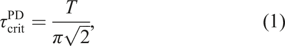
The critical delay can be increased by employing other than PD feedback. For instance, if the feedback involves acceleration (PDA feedback), then the critical delay can be increased to $τ_{c r i t}^{P D A} = \sqrt{2} τ_{c r i t}^{P D}$ (Sieber and Krauskopf, 2005). Alternatively, if the delays of the proportional and the derivative terms are detuned, then the critical delay increases to $τ_{c r i t}^{d P D} \approx 1.47 τ_{c r i t}^{P D}$ (Sieber and Krauskopf, 2005). Another alternative way to increase the critical delay is the application of fractional order control: in case of PD^μ feedback, $τ_{c r i t}^{{P D}^{μ}} \approx 1.12 τ_{c r i t}^{P D}$ (Balogh and Insperger, 2018).

Introducing fractional-order derivative in the feedback loop allows us to exploit the time history starting from some initial time to the current time instant. This can be seen from the most frequently used definitions of fractional derivative: the Riemann–Liouville fractional derivative, the Caputo fractional derivative and the Grünwald–Letnikov fractional derivative. All of these definitions of the fractional derivative resembles a distributed delay term. Implementation of fractional-order feedback is, therefore, computationally demanding. Fractional-order differential equations can be treated similarly to integer-order differential equations, although there are some concepts and techniques that need to be generalized (Podlubny, 1998).

In this paper, we consider the PD^μ control of an inverted pendulum with different delays in the proportional and the fractional derivative terms. This concept gives a transition between two special cases already investigated in the literature.

1. Detuned PD feedback (the case μ = 1) was investigated in Sieber and Krauskopf (2005).

2. Fractional-order PD feedback without delay detuning (the case τ_p = τ_d) was investigated in Balogh and Insperger (2018).

Here, we combine these two concepts and derive the admissible feedback delay for the detuned fractional-order PD feedback.

The different delays originate in the different sensory systems used for the perception of position and velocity. In engineering applications, the operation of position and velocity sensors is different; therefore, they typically result in different delays in the feedback loop. In human postural balance, as a biological application, position and velocity information are obtained by the static and dynamic receptors of the inner ear, which induces that the corresponding delays are different. When the velocity is calculated as a discrete difference of the position, then signal processing introduces an extra delay.

The characteristic function of the system under investigation reads

D (s) = s^{2} - a_{0} + k_{p} e^{- s τ_{p}} + k_{d} s^{μ} e^{- s τ_{d}},

(2)

where a₀ > 0 is the plant parameter, τ_p > 0 and τ_d > 0 are the feedback delays, and 0 < μ < 2 is the order of the fractional derivative term. System (2) is said to be stabilizable for given delays τ_p and τ_d if there exist some control gains k_p, k_d and derivative order μ for which (2) is stable (i.e., (2) has roots with negative real parts only). The goal of this paper is to determine the critical delay τ_crit as the maximum of min{τ_p, τ_d} such that (2) is still stabilizable.

This definition of the critical delay is of interest because one can also think of (2) as a control system with a single control-loop latency τ and some additional delays (or delay detunings) δ_p and δ_d. This concept leads to

D (s) = s^{2} - a_{0} + k_{p} e^{- s (τ + δ_{p})} + k_{d} s^{μ} e^{- s (τ + δ_{d})}

(3)

with δ_p ≥ 0 and δ_d ≥ 0. In this sense, the system is stabilizable for a given τ if there exist some k_p, k_d, μ, and δ_p, δ_d for which (3) is stable. Thus, the additional delays are introduced in hopes of improving the stabilizability of the original single-delay system. In the following, we refer to (3) as detuned PD^μ feedback. The goal of the paper can be rephrased as follows. We are looking for the critical delay τ_crit for the detuned PD^μ feedback (3) such that if τ < τ_crit, then (3) can be stabilized with an appropriate choice of k_p, k_d, μ, and δ_p, δ_d ≥ 0.

The paper is organized as follows. After some preliminary thoughts, some special cases are discussed in Special Cases. In Stabilizability Analysis, stabilizability diagrams are constructed and their change is analyzed with respect to the order of the fractional derivative in order to find the critical delay.

Preliminaries

Stability of linear time-invariant fractional-order time delay systems can be investigated using their characteristic function: the system is BIBO (bounded-input bounded-output) stable if and only if the roots of the characteristic function have negative real part on the first Riemann sheet (Bonnet and Partington, 2002; Matignon, 1996; Monje et al., 2010). Consequently, the D-subdivision method can be applied to (2) as follows.

Substitution of s = 0 and s = ±iω, ω > 0 into D(s) = 0 gives the D-curves

\begin{array}{c} s = 0 : & k_{p} = a_{0}, k_{d} \in R, \end{array}

(4)

\begin{array}{c} s = \pm i ω : & {\begin{array}{c} k_{p} = (a_{0} + ω^{2}) \frac{\sin (\frac{μ π}{2} - τ_{d} ω)}{\sin (\frac{μ π}{2} - (τ_{d} - τ_{p}) ω)}, \\ k_{d} = (a_{0} + ω^{2}) \frac{\sin (τ_{p} ω)}{ω^{μ} \sin (\frac{μ π}{2} - (τ_{d} - τ_{p}) ω)} . \end{array} \end{array}

(5)

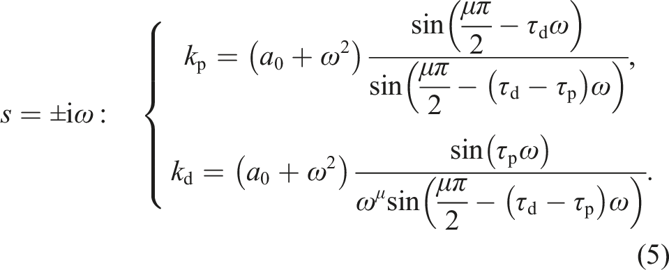
The D-curves bound the parameter regions in the plane (k_p, k_d) where the number of unstable characteristic roots is constant. Stable regions (zero unstable characteristic roots) can be determined by the argument principle (Merrikh-Bayat, 2013; Wang et al., 2011). When the delays increase, then the stable regions typically shrink and disappear. There is a critical delay $τ_{c r i t}^{{d P D}^{μ}}$ : if $\min {τ_{p}, τ_{d}} > τ_{c r i t}^{{d P D}^{μ}}$ , then the system (2) cannot be stabilized by any triplet (k_p, k_d, μ). The goal of this paper is to determine the stabilizability boundaries in the plane (τ_p, τ_d) and to find $τ_{c r i t}^{{d P D}^{μ}}$ .

Special cases

Special cases can be defined either by setting the fractional order μ to integer or by setting τ_p = τ_d.

Integer-order controllers: μ = 0, μ = 1 and μ = 2

Special cases μ = 0 and μ = 1 were already analyzed in Sieber and Krauskopf (2005). If μ = 0 and τ_p ≠ τ_d then one gets the proportional minus delay (PMD) controller of Sieber and Krauskopf (2005). In this case, a non-semisimple triple-zero eigenvalue occurs at the limit of stabilizability, which corresponds to the parameter combinations

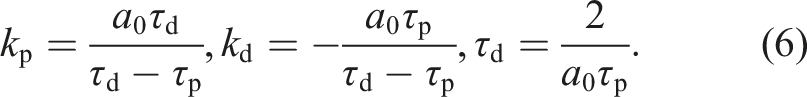
k_{p} = \frac{a_{0} τ_{d}}{τ_{d} - τ_{p}}, k_{d} = - \frac{a_{0} τ_{p}}{τ_{d} - τ_{p}}, τ_{d} = \frac{2}{a_{0} τ_{p}} .

(6)

Equation (6) gives a hyperbolic relation between the delays (see Figure 1(a)). Note that τ_d is a strictly decreasing function of τ_p, therefore min{τ_p, τ_d} is maximal if τ_p approaches τ_d. The limit case τ_p → τ_d would give the critical delay $τ_{c r i t}^{P M D} = \sqrt{2 / a_{0}} = τ_{c r i t}^{P D}$ . However, at the limit case τ_p = τ_d, the control gains k_p and k_d are singular. This limit case corresponds to a proportional feedback with a single delay τ = τ_p = τ_d, which cannot stabilize the inverted pendulum as explained below. Due to the necessary condition in Kharitonov et al. (2005), if the quasipolynomial f(s) = e^sτ(s² − a₀) + k_p is stable, then f′(s) = e^sτ(τs² + 2s − a₀τ) should also be stable. However, this is not true, since a₀ > 0 and τ > 0. Hence, f(s) cannot be stable. Alternatively, it can be seen that the inverted pendulum cannot be stabilized by delayed PD feedback if k_d = 0 since k_d > a₀τ is a necessary condition for stabilization (Insperger and Milton, 2021; Stepan, 2009).

Figure 1.

The stabilizability boundaries and multiplicity conditions in the plane (τ_p, τ_d) if μ = 0 (a), μ = 1 (b), and μ = 2 (c) with a₀ = 2.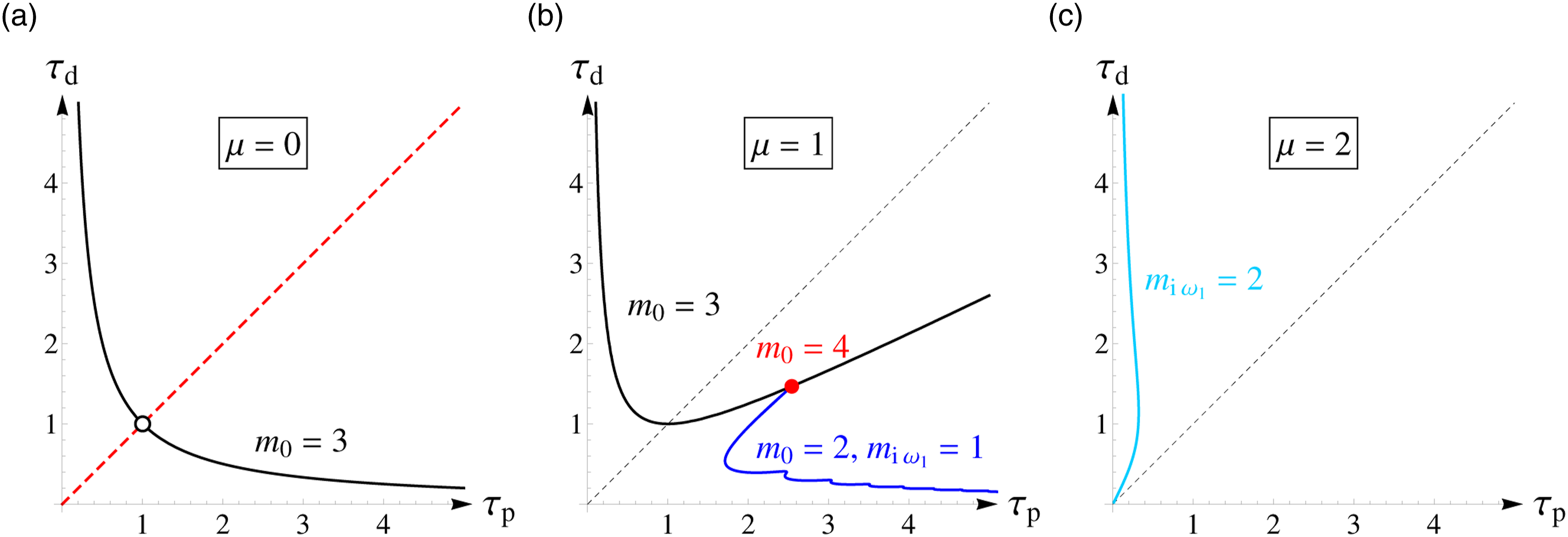

The case μ = 1 corresponds to the detuned PD (dPD) controller in Sieber and Krauskopf (2005), where it was shown that the critical delay can be extended to $τ_{c r i t}^{d P D} \approx 1.47 τ_{c r i t}^{P D}$ . The stabilizability boundaries for this case were given in Balogh et al. (2022b) and are shown in Figure 1(b). The critical parameter combination is indicated by a red dot, where there is a root s = 0 with multiplicity 4 (m₀ = 4). At this point, the ratio of the delays is $τ_{p} / τ_{d} = \sqrt{3}$ . This critical point is given as the intersection of two parametric curves indicated by black and blue lines in Figure 1(b). The black curve is associated with a triple root s = 0 (m₀ = 3) and the blue curve is associated with a combination of a double root s = 0 (m₀ = 2) and a pair of purely imaginary roots $(m_{i ω_{1}} = 1)$ . For further details in this case, see Balogh et al. (2022b).

The case μ = 2 corresponds to a detuned proportional-acceleration (dPA) feedback, that is, a detuned PDA feedback with k_d = 0. If τ_p = τ_d, then the system cannot be stabilized similarly to the case μ = 0. If delay detuning is allowed, then the system can be stabilized and the critical delay is $τ_{c r i t}^{d P A} \approx 0.32 τ_{c r i t}^{P D}$ . The stabilizability boundary shown in Figure 1(c) was derived using the methods explained later in Constructing Stabilizability Diagrams in the Plane (τ_p, τ_d).

A special combination of the cases μ = 1 and μ = 2 gives the detuned PDA feedback, which was investigated in Balogh et al. (2022b) in terms of stabilizability boundaries. The idea of integer-order delayed PD and derivative-acceleration controllers was also addressed in Wang and Xu (2017) in the case of the damped harmonic oscillator.

PD^μ controller with a single delay

The special case τ_p = τ_d = τ was already investigated in Balogh and Insperger (2018). The stabilizable region was derived in the plane of the dimensionless parameters a = a₀τ² and μ (see Figure 2(a)). Using the D-subdivision technique, one can observe four types of loss of stabilizability. These geometric conditions can directly be translated into the multiplicity conditions shown in Figure 2(b). The stabilizability boundary consists of three segments:

Figure 2.

Stabilizable region of (2) if τ_p = τ_d = τ with a = a₀τ² (a). The stabilizability boundaries and multiplicity conditions in the plane (μ, τ) if a₀ = 2 (b).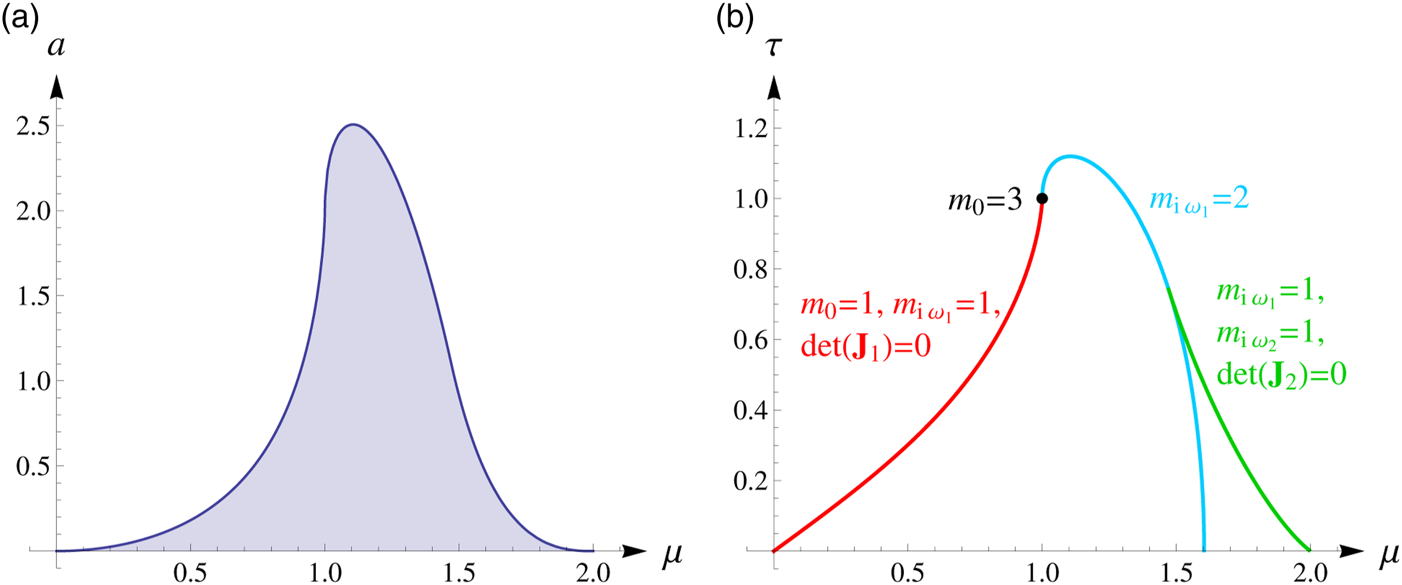

1. There is a single zero root (s = 0) and a single pair of purely imaginary roots (s = ± iω₁, ω₁ > 0) with an additional condition

\det (J_{1}) = 0,

(7)

where J₁ is the Jacobian matrix of equations

D (0) = 0, R e D (i ω_{1}) = 0, I m D (i ω_{1}) = 0

(8)

with respect to k_p, k_d, and ω₁ (for more details, see Appendix 1). Thus, equation (7) represents the singularity of the Jacobian matrix J₁. The geometric interpretation of this condition is the tangency of the D-curves at the critical point similarly to the case shown in Figure 3(a). This segment is indicated by red line in Figure 2(b). A similar type of stabilizability boundary can be seen in Michiels and Niculescu (2007) or in Balogh et al. (2022b) (where this phenomenon is referred to as a turning point).

2. There is a double pair of purely imaginary roots shown by blue line in Figure 2(b). The corresponding geometric interpretation is a loop-cusp transition of the stable region similarly to the case shown in Figure 3(c).

3. There are two pairs of purely imaginary roots (s = ±iω₁, ω₁ > 0 and s = ±iω₂, ω₂ > 0) with an additional condition

\det (J_{2}) = 0,

(9)

where J₂ is the Jacobian matrix of equations

\begin{array}{c} R e D (i ω_{1}) & = 0, I m D (i ω_{1}) = 0, \\ R e D (i ω_{2}) & = 0, I m D (i ω_{2}) = 0 \end{array}

(10)

with respect to k_p, k_d, ω₁, and ω₂. In this case, the stable region disappears as the complex root boundary crosses itself tangentially similarly to the case shown in Figure 3(f). This stabilizability boundary is shown by green line in Figure 2(b).

Figure 3.

Stability charts: Types of loss of stabilizability and the corresponding multiplicity conditions. Here, 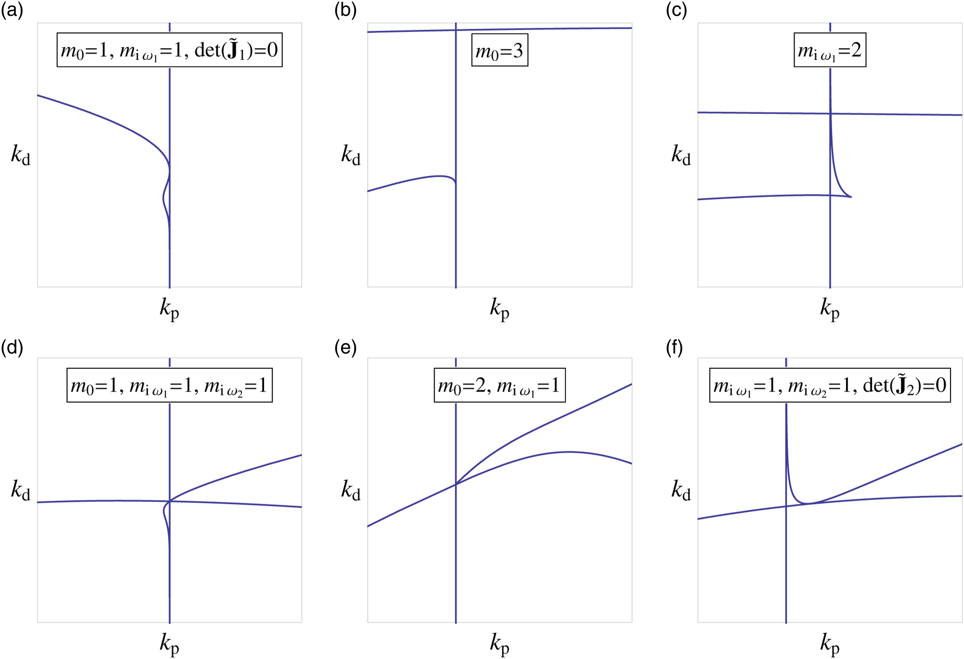${\tilde{J}}_{1}$ is the Jacobian matrix of (8) with respect to k_p, k_d, ω₁.

At the connection point of segments 1 and 2, there is a triple zero root (s = 0) similarly to the case shown in Figure 3(b).

Stabilizability analysis

The main goal is to determine the stabilizable region in the plane (τ_p, τ_d) for the general case (0 < μ < 2). Then, the critical delay for (3) can also be obtained by analyzing the changes of the stabilizability boundaries for varying μ.

Constructing stabilizability diagrams in the plane (τ_p, τ_d)

Stabilizability can be investigated by observing the change of the stable parameter region with respect to the change of some other parameters. Figure 4 shows an example of how the stable region in the parameter plane (k_p, k_d) (bounded by the loop of (5)) changes as parameter τ_p is increased if μ = 1.2 and τ_d = 0.58 with a₀ = 2. The stable region shrinks to a single point if τ_p ≈ 1.19. At this critical point, the characteristic function has a distinct pair of purely imaginary roots since the complex root boundary (5) touches itself. The tangency at the critical point imposes another condition, namely, $\det ({\tilde{J}}_{2}) = 0$ . Here, ${\tilde{J}}_{2}$ is the Jacobian matrix of (10) with respect to k_p, k_d, ω₁, and ω₂.

Figure 4.

Stability charts of (2) if μ = 1.2 and τ_d = 0.58 with a₀ = 2. The critical point corresponds to 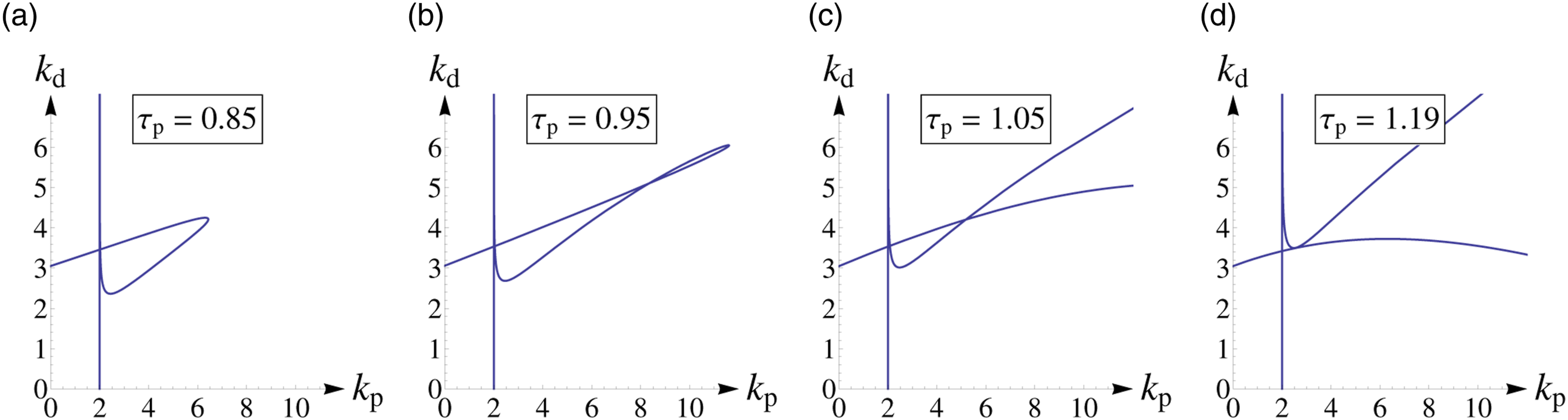$m_{i ω_{1}} = 1$ , $m_{i ω_{2}} = 1$ , and $\det ({\tilde{J}}_{2}) = 0$ .

The multiplicity conditions in PD^μ Controller With a Single Delay give a more uniform description of the stabilizability boundaries compared to that of Balogh and Insperger (2018). Furthermore, the techniques in PD^μ Controller With a Single Delay can also be applied if τ_p ≠ τ_d. That is, the stabilizability boundaries can be obtained following the steps below.

1. Geometric conditions at the limit of stabilizability should be detected by D-subdivision as shown in Figure 4. Different parameter regions exhibit different types of loss of stabilizability. Here, six different geometric conditions are distinguished which are represented in Figure 3.

2. Geometric conditions should be translated into multiplicity conditions. The multiplicity conditions corresponding to the critical points are also shown in Figure 3. Note that multiplicity condition $m_{i ω_{1}} = 1$ , $m_{i ω_{2}} = 1$ , $m_{i ω_{3}} = 1$ is also possible algebraically but was not found to be relevant.

3. Each multiplicity condition gives a nonlinear system of M + 3 equations for variables k_p, k_d, τ_p, τ_d, μ, and ω_i, i = 1, …, M for some M that could also be 0. If μ and τ_p or τ_d are fixed, then this system of equations could be solved for the rest of the variables. These nonlinear systems of equations are linear in k_p and k_d, therefore reduced systems of equations can be obtained by solving two of the equations for k_p and k_d. Then, only the remaining equations have to be solved numerically.

4. A solution can be represented by a point in the plane (τ_p, τ_d) for a fixed μ. In order to find an initial solution, a critical point and the corresponding parameter values (obtained by D-subdivision) can be used as an initial guess. If the reduced system of equations consists of less than three equations, then contour plots of these equations also give insight into the possible initial solutions. Then, such a (initial) point can be extended to a curve (i.e., to a stabilizability boundary) by using numerical continuation. Pseudo-arclength continuation allows us to follow the solution curve even if the tangent is vertical (or horizontal).

An example for the stabilizability boundaries is shown in Figure 5 for μ = 1.2. Two types of loss of stabilizability may show up: a pair of purely imaginary roots with multiplicity two indicated by blue line; and two pairs of distinct purely imaginary roots with and additional condition $\det ({\tilde{J}}_{2}) = 0$ indicated by green line.

Figure 5.

The stabilizability boundaries and multiplicity conditions in the plane (τ_p, τ_d) if μ = 1.2 with a₀ = 2.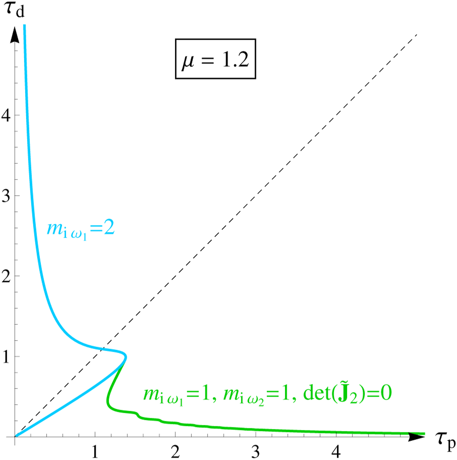

Changes in stabilizability for varying μ

Figure 6 shows the stabilizability boundaries in the plane (τ_p, τ_d) for different values of μ in the neighborhood of μ = 1. The stabilizable region can be extended compared to the detuned PD controller (μ = 1) by choosing an appropriate value of the fractional order μ. The line $τ_{d} = τ_{p} / \sqrt{3}$ passes through the critical point of the case μ = 1 and separates the plane (τ_p, τ_d) into two regions. If $τ_{d} < τ_{p} / \sqrt{3}$ , then it can be beneficial to use a fractional derivative of order less than 1. On the other hand, if $τ_{d} > τ_{p} / \sqrt{3}$ , then the fractional-order derivatives of order greater than 1 may show better stabilizability properties.

Figure 6.

The stabilizability boundaries in the plane (τ_p, τ_d) if μ ≤ 1 (a) and μ ≥ 1 (b) with a₀ = 2. Stabilizable regions are to the left of the curves.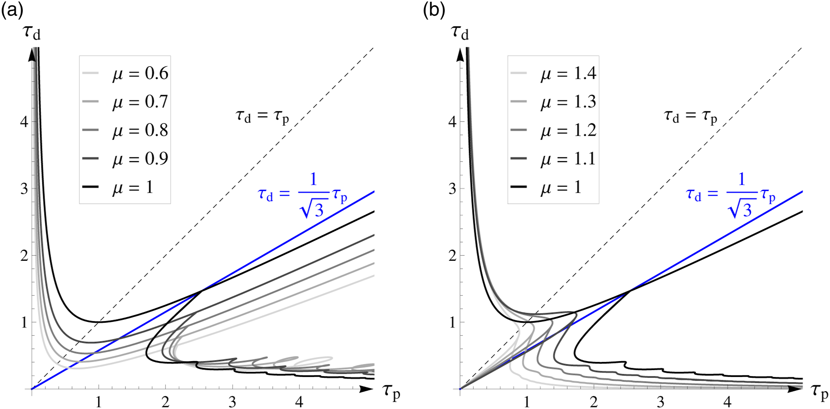

Critical delay in the sense of detuned fractional-order PD feedback

We can draw more conclusions from the stabilizability diagrams. For every μ, we can find a point in the stabilizable region where the minimum of τ_p and τ_d is maximal. The path of this point is shown by red line in Figure 7(a) if μ ≤ 1. In Figure 7(b), the critical delay (related to the detuned fractional-order PD feedback (3)) is shown as a function of μ in the left neighborhood of μ = 1.

Figure 7.

The path of the critical point in the plane (τ_p, τ_d) if μ ≤ 1 (a) and the critical delay for 0.99 ≤ μ ≤ 1 (b) with a₀ = 2.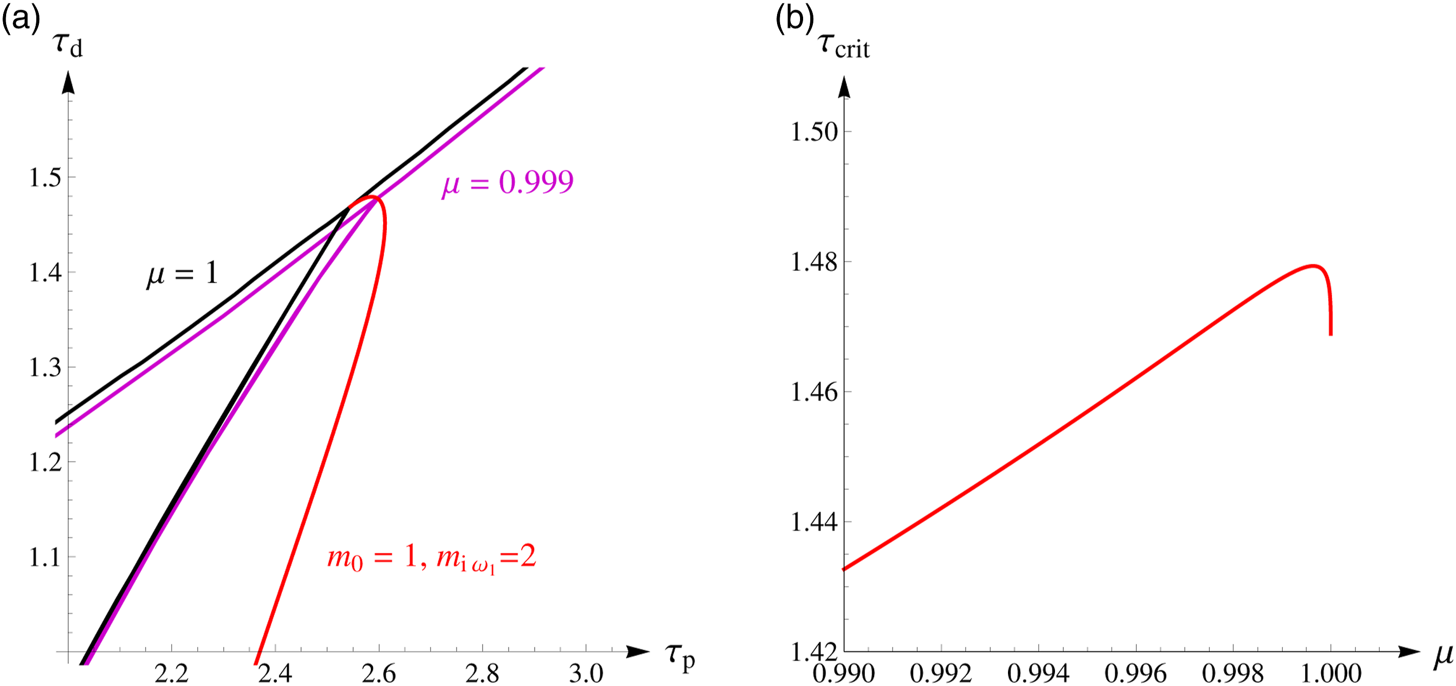

The largest admissible delay is obtained for μ = 0.999,637. In this case, the critical delay is $τ_{c r i t}^{{d P D}^{μ}} = 1.00778 τ_{c r i t}^{d P D}$ (see Figure 7). Hence, the critical delay can be increased only to an extremely small extent by detuning the delays.

Conclusions

Table 1 shows how the numerical values of the critical delay compare to each other in the case of the PD, detuned PD, fractional-order PD and detuned fractional-order PD controllers. As can be seen, the critical delay for the detuned PD^μ controller is slightly larger than that of the detuned PD controller, namely, by a factor of 1.00,778. Although this gain in the critical delay is practically insignificant, there are some cases when fractional-order feedback may still be beneficial. If there are some constraints on the delays τ_p and τ_d, then fractional-order feedback may stabilize a system that cannot be stabilized by integer-order feedback. This can be seen by the extended stabilizable region for different derivative orders μ in Figure 6.

Table 1.

Critical delays for a₀ = 2.

	PD	Detuned PD	PD^μ	Detuned PD ^μ
τ _crit	1	1.468	1.120	1.479

An extension of the admissible delays is also possible by introducing detuned PDA feedback described by

D (s) = s^{2} - a_{0} + k_{p} e^{- s τ_{p}} + k_{d} s e^{- s τ_{d}} + k_{a} s^{2} e^{- s τ_{a}},

(11)

where k_a is the acceleration feedback gain, and τ_a is the delay for the acceleration feedback. In this case, the critical delay can be increased by a factor of 1.180 compared to the detuned PD case (Balogh et al., 2022b). A further extension might be possible by employing detuned PD^μD^ρ feedback described by

D (s) = s^{2} - a_{0} + k_{p} e^{- s τ_{p}} + k_{d 1} s^{μ} e^{- s τ_{d 1}} + k_{d 2} s^{ρ} e^{- s τ_{d 2}},

(12)

where 0 < μ < 2 and 0 < ρ ≤ 2 are the orders of the fractional derivatives. The critical delays of some special cases of PD^μD^ρ feedback are listed in Table 2. The critical delay for detuned PDA feedback is

τ_{c r i t}^{d P D A} = \sqrt{3} τ_{c r i t}^{P D}

(Balogh et al., 2022b). For single-delay PD^μD^ρ feedback, it is

τ_{c r i t}^{{P D}^{μ} D^{ρ}} = 1.468 τ_{c r i t}^{P D}

(Balogh and Insperger, 2018). The critical delay for detuned PD^μD^ρ feedback is still an open question.

Table 2.

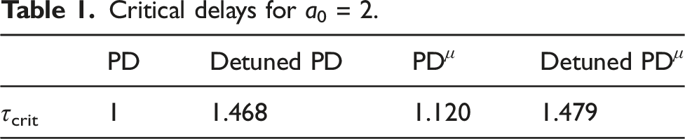
Critical delays for a₀ = 2.

	PD	PDA	Detuned PDA	PD^μD^ρ	Detuned PD^μD^ρ
τ _crit	1	1.414	1.732	1.468	?

Footnotes

Declaration of conflicting interests

The author(s) declared no potential conflicts of interest with respect to the research, authorship, and/or publication of this article.

Funding

The author(s) disclosed receipt of the following financial support for the research, authorship, and/or publication of this article: The research reported in this paper has been supported by Project no. TKP-9-8/PALY-2021 provided by the Ministry of Culture and Innovation of Hungary from the National Research, Development and Innovation Fund, financed under the TKP2021-EGA funding scheme, by the Nemzeti Kutatási Fejlesztési és Innovációs Hivatal (Grant nos. NKFI-K138621 and BME-NVA-02) and by the ÚNKP-22-3-II-BME-98 New National Excellence Program of the Ministry for Culture and Innovation from the source of the Nemzeti Kutatási Fejlesztési és Innovációs Hivatal.

ORCID iDs

Tamas Balogh

Tamas Insperger

Appendix

References

Balogh

Boussaada

Insperger

, et al. (2022a) Conditions for stabilizability of time-delay systems with real-rooted plant. International Journal of Robust and Nonlinear Control 32(6): 3206–3224.

Balogh

Insperger

(2018) Extending the limits of stabilizability of systems with feedback delay via fractional-order PD controllers. IFAC-PapersOnLine 51(14): 265–270.

Balogh

Varszegi

Insperger

(2022b) On the admissible control-loop delay for the inverted pendulum subject to detuned PDA feedback. Journal of Sound and Vibration 529: 116898.

Bonnet

Partington

(2002) Analysis of fractional delay systems of retarded and neutral type. Automatica 38(7): 1133–1138.

Boussaada

Niculescu

El Ati

, et al. (2020) Multiplicity-induced-dominancy in parametric second-order delay differential equations: analysis and application in control design. ESAIM: Control, Optimisation and Calculus of Variations 26: 57. DOI: 10.1051/cocv/2019073

Boussaada

Tliba

Niculescu

, et al. (2018) Further remarks on the effect of multiple spectral values on the dynamics of time-delay systems. Application to the control of a mechanical system. Linear Algebra and its Applications 542: 589–604.

Boussaada

Ünal

Niculescu

(2016) Multiplicity and stable varieties of time-delay systems: a missing link. In: Proceeding of the 22nd International Symposium on Mathematical Theory of Networks and Systems, Minneapolis, MN, July 12-15, 2016.

Castillo-Zamora

Boussaada

Benarab

, et al. (2023) Time-delay control of quadrotor unmanned aerial vehicles: a multiplicity-induced-dominancy-based approach. Journal of Vibration and Control 29(11–12): 2593–2608.

Insperger

Milton

(2021) Delay and Uncertainty in Human Balancing Tasks. Berlin, Germany: Springer.

10.

Kharitonov

Niculescu

Moreno

, et al. (2005) Static output feedback stabilization: necessary conditions for multiple delay controllers. IEEE Transactions on Automatic Control 50(1): 82–86.

11.

Lewis

Torczon

Trosset

(2000) Direct search methods: then and now. Journal of Computational and Applied Mathematics 124(1–2): 191–207.

12.

Matignon

(1996) Stability results for fractional differential equations with applications to control processing. Computational Engineering in Systems Applications 2: 963–968.

13.

Merrikh-Bayat

(2013) General formula for stability testing of linear systems with fractional-delay characteristic equation. Central European Journal of Physics 11(6): 855–862.

14.

Michiels

Niculescu

(2007) Stability and Stabilization of Time-Delay Systems: An Eigenvalue-Based Approach. Philadelphia, PA: SIAM.

15.

Molnar

Balogh

Boussaada

, et al. (2021) Calculation of the critical delay for the double inverted pendulum. Journal of Vibration and Control 27(3-4): 356–364.

16.

Molnar

Insperger

(2016) On the robust stabilizability of unstable systems with feedback delay by finite spectrum assignment. Journal of Vibration and Control 22(3): 649–661.

17.

Monje

Chen

Vinagre

, et al. (2010) Fractional-Order Systems and Controls: Fundamentals and Applications. Berlin, Germany: Springer Science and Business Media.

18.

Podlubny

(1998) Fractional Differential Equations: An Introduction to Fractional Derivatives, Fractional Differential Equations, to Methods of Their Solution and Some of Their Applications. Amsterdam, Netherlands: Elsevier.

19.

Shi

Zhang

(2020) Tuning of digital PID controllers using particle swarm optimization algorithm for a CAN-based DC motor subject to stochastic delays. IEEE Transactions on Industrial Electronics 67(7): 5637–5646.

20.

Qin

Zhong

, et al. (2014) Control experiments on time-delayed dynamical systems. Journal of Vibration and Control 20(6): 827–837.

21.

Shi

Zhang

(2021) Fault diagnosis of an autonomous vehicle with an improved SVM algorithm subject to unbalanced datasets. IEEE Transactions on Industrial Electronics 68(7): 6248–6256.

22.

Sieber

Krauskopf

(2005) Extending the permissible control loop latency for the controlled inverted pendulum. Dynamical Systems 20(2): 189–199.

23.

Stepan

(1989) Retarded Dynamical Systems: Stability and Characteristic Functions. Harlow, UK: Longman.

24.

Stepan

(2009) Delay effects in the human sensory system during balancing. Philosophical Transactions of the Royal Society A: Mathematical, Physical & Engineering Sciences 367(1891): 1195–1212.

25.

Wang

Shi

(2011) Stability test of fractional-delay systems via integration. Science China Physics, Mechanics & Astronomy 54(10): 1839–1846.

26.

Wang

(2017) Sway reduction of a pendulum on a movable support using a delayed proportional-derivative or derivative-acceleration feedback. Procedia IUTAM 22: 176–183.

27.

Stepan

Wang

(2017) Balancing a wheeled inverted pendulum with a single accelerometer in the presence of time delay. Journal of Vibration and Control 23(4): 604–614.

Extending the admissible control-loop delays for the inverted pendulum by fractional-order proportional-derivative controller

Abstract

Keywords

Introduction

Preliminaries

Special cases

Integer-order controllers: μ = 0, μ = 1 and μ = 2

PD μ controller with a single delay

Stabilizability analysis

Constructing stabilizability diagrams in the plane (τp, τd)

Changes in stabilizability for varying μ

Critical delay in the sense of detuned fractional-order PD feedback

Conclusions

Footnotes

Declaration of conflicting interests

Funding

ORCID iDs

Appendix

References

PD^μ controller with a single delay

Constructing stabilizability diagrams in the plane (τ_p, τ_d)