Robust trajectory tracking control design for the robotic arm with uncertainty and experimental validation

Abstract

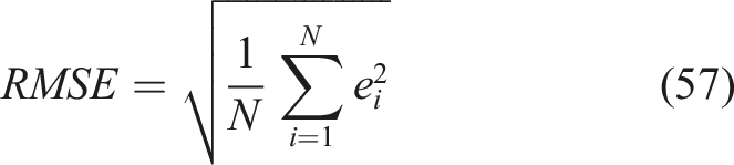
The robotic arm is a complicated system with multiple inputs and outputs, strong coupling, containing uncertainties and nonlinearities. This study proposes a new practical robust control method based on the dynamics model and tracking error, including a model- and error-based proportional-differential feedback term and an error-based robust term. Specifically, the dynamics of the system are modeled using the Lagrangian method. Uncertainties are presumed to be time-varying but limited. Based on the Lyapunov method, the proposed controller has theoretically demonstrated the controlled system with uniform boundedness (UB) and uniform ultimate boundedness (UUB). Furthermore, the radius of the ultimately bounded hypersphere is arbitrarily small based on selecting appropriate design parameters. Based on the two-degree-of-freedom (2-DOF) planar robotic arm experimental platform, the self-developed rapid controller prototype CSPACE-RT is intended to eliminate tedious programming or debugging, significantly simplifying the experimental process. Finally, numerical simulation and experiment results verified the excellent control performance of the suggested controller.

Keywords

robust control robotic arm uncertainty Lyapunov method trajectory tracking dynamic performance

1. Introdution

With the rapid development of digital computer technology, robotics has become one of the focused research fields nowadays (Dean-Leon et al., 2017; Sumartojo and Lugli, 2022; Lee et al, 2022). Robots are designed to assist or replace humans in completing actual work and play an essential part in manufacturing. As the most crucial execution terminal of a robot, the robotic arm is the key to completing a specific task. Robotic arms are increasingly employed in numerous fields, including industrial manufacturing (Alandoli et al., 2022), aerospace (Santos et al., 2022), marine exploration (Sivčev et al., 2018), medical surgery (Troccaz et al., 2019), and agricultural harvesting (Tang et al., 2020) for the advantages of simple structure, high space utilization, ample working space, high flexibility, and multiple postures. The different needs of various fields have posed higher challenges to the motion control of robotic arm systems. Improving the stability, accuracy, and speed of the robotic arm system control to perform complex and delicate operations is critical.

However, the robotic arm system is a typical nonlinear electromechanical system with multiple inputs and outputs, strong coupling, and uncertainty (Zhai and Xu, 2021). When there are modeling errors, uncertainties and unknown perturbations in the robotic arm system, it is challenging to provide high-accuracy trajectory tracking control of the robotic arm for controllers without robustness. Therefore, designing a control scheme that can effectively resist uncertainties and guarantee that the robotic arm system achieves high-precision motion is essential.

Achieving trajectory tracking of the robotic arm requires designing an excellent controller to ensure the dynamic performance of the system. Many contributions have been published addressing the control challenges for nonlinear systems. The typical control methods are proportion-integration-differentiation (PID) control (Ang et al., 2005; Gaidhane et al., 2019; Zamani and Etedali, 2023), active disturbance rejection control (ADRC) (Han, 2009; Chen and Chen, 2021; Fareh et al., 2021), and adaptive control (Villani et al., 1999; Nikdel et al. 2017; Shi et al., 2021). Conventional PID control is still extensively utilized in real industrial realms since its simplicity and lack of dependence on the system model. However, the single PID control algorithm with low control accuracy and poor robustness is challenging to be applied to nonlinear systems. Inherited from PID, ADRC is widely used because of its simple implementation, excellent performance of control, and resistance to interference. ADC maintains the system in a better state by adjusting the control law through system error instantly. It, however, needs a considerable amount of computation and requires a high degree of real-time performance of the system.

Many advanced control algorithms have been proposed based on the increasing computer data processing power. In Ref. Ma and Huang (2020), a proposed novel adaptive law manipulator control scheme that approximates the neural network to the unmodeled part of the dynamics is presented. Yin et al. (2021) uses fuzzy logic system and adaptive law to compensate the uncertainty of high frequency and low frequency, respectively. As a result, the trajectory tracking performance is better. In Ref. Lai et al. (2017), the pose of the planar four-link underdriven robotic arm at different stages of motion is optimized using genetic algorithms and separate controllers are designed.

In addition to the above control methods, robust control is commonly utilized in actual engineering to compensate for the structural and non-structural uncertainty portions of the system. It enables the system to achieve a relatively good control effect in the case of a bounded uncertainty range. The main robust control methods are H_∞ control (Xu and Chen, 2002; Figueredo et al., 2021), sliding mode control (SMC) (Islam and Liu, 2011; Baek et al., 2016; Aboserre and El-Badawy, 2021), and adaptive robust control (ARC) (Solanes et al., 2018; Yin and Pan, 2018; Rad et al., 2020). Whereas H_∞ control takes uncertainty into account, the method is not model-based. Thus, it is not easy to achieve high speed/high precision in practice. Theoretically, SMC is completely robust to uncertainty. But, its properties can lead to high frequency chattering in the system. Another way to improve control is by using the state, input and output information of the controlled object system, ARC adjusts the structure or parameters of the controller online. This needs the design of the adaptive law and is relatively complex in practical applications.

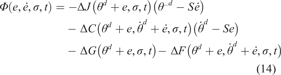
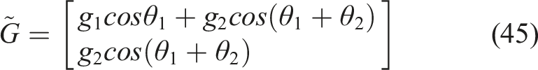
A new practical model- and error-based robust controller is proposed considering the uncertainty of the internal parameters of the system and the unknown external perturbations. The proposed controller comprises a model- and error-based proportional-differential (PD) control term and an error-based robust control term. Specifically, the nominal and uncertain parts constitute the dynamics model of the system. The cumulative influence of all uncertain parts on the system is represented by the function $Φ (e, \dot{e}, σ, t)$ and its upper bound is considered to be the function $ρ (e, \dot{e}, σ, t)$ . The Lyapunov minimax approach is used to theoretically verify that the suggested controller with uniform boundedness and uniform ultimate boundedness, hence assuring the stability of the controlled object system. The designed controller inherits conventional PD control and deterministic robust control. It has robustness against the effects of uncertainty on the system based on high-precision trajectory tracking control.

The proposed controller has the advantages of a simple structure, a small number of parameters, and a simple parameter adjustment process compared with other robust controllers, which is easier to apply to practical engineering.

This paper proposes a high-precision trajectory tracking control scheme for the robotic arm system with the following main contributions.

1. The proposed controller has the advantages of both traditional PD control and robust control, which guarantees accurate trajectory tracking of the robotic arm system for unknown uncertainties of system parameters.

2. By constructing an effective Lyapunov function, the proposed controller is theoretically verified to have uniform boundedness and uniform ultimate boundedness, ensuring the stability of the practical system.

3. The self-developed rapid control prototype CSPACE-RT is intended to improve experimental efficiency. Numerical simulations and experimental results of the suggested control algorithm are given on the 2-DOF planar robotic arm experimental platform. A comparative analysis with other control algorithms is performed. It is concluded that the suggested control approach can provide the system with high-accuracy trajectory tracking and powerfully robust performance.

This paper is organized as follows. Section 2 constructs the dynamics model of the robotic arm nonlinear system. Section 3 outlines the design process of the proposed controller and verifies its stability theoretically. Section 4 presents numerical simulations and experimental validation of the proposed controller and compares the results with PID and MEBPD control algorithms. Section 5 gives conclusions for the work in the whole paper.

2. The derivation of the dynamics model

The dynamics mainly research the relationship between the force and the kinematics of the research object during the movement. The dynamic model must be established and analyzed for a complex nonlinear robot system to realize real-time control.

The main research methods of robot dynamics are the Lagrangian method, Newton-Euler method, Gauss method, etc. Among them, the Lagrangian dynamic algorithm is an energy-based dynamic method. This approach requires identifying the overall energy characteristics of the system rather than examining its interior intricacies. Therefore, we select the Lagrangian technique to develop the dynamic model of the robotic arm.

For any robotic arm system with n-DOF, the Lagrangian equation is as follows:

\frac{d}{d t} (\frac{\partial L (θ, \dot{θ}, t)}{\partial \dot{θ_{i}}}) - \frac{\partial L (θ, \dot{θ}, t)}{\partial θ_{i}} = τ_{i} (t), i = 1,2, \dots, n

(1)

where L (⋅) is the Lagrangian operator, which can be expressed as equation (2). θ_i,

\dot{θ_{i}}

, and τ_i are the generalized coordinates, the velocity and control force of the ith joint, respectively.

L (θ, \dot{θ}, t) = K (θ, \dot{θ}, t) - P (θ, t)

(2)

where the kinetic energy of the system is

K (θ, \dot{θ}, t)

and P (θ, t) is the potential energy of the system.

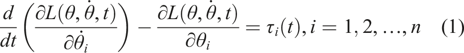
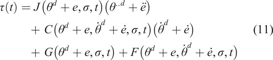
Considering that the robotic arm may be subjected to unknown external perturbations like load variation and friction in the working environment. Combining equations (1) and (2), the general dynamics model of the n-DOF robotic arm can be written as

J (θ, t) \ddot{θ} + C (θ, \dot{θ}, t) \dot{θ} + G (θ, t) + F (θ, \dot{θ}, t) = τ (t)

(3)

where J (⋅) ∈ R^n×n, C (⋅) ∈ R^n×n, G (⋅) ∈ Rⁿ, F (⋅) ∈ Rⁿ are the symmetric inertia matrix of the system, the Coriolis and centrifugal force matrix, the gravity vector and the friction force, respectively. θ(t) ∈ Rⁿ,

\dot{θ} (t) \in R^{n}

, and

\overset{. .}{θ} (t) \in R^{n}

are the robotic arm joint position, velocity, and acceleration, respectively. And τ(t) ∈ Rⁿ is the output control torque.

An appropriate friction model is crucial for modeling the dynamics of the robotic arm. The accuracy of the friction model of the system will greatly reduce chattering and significantly increase the trajectory accuracy during the motion of the robotic arm (Liu et al., 2016). The traditional friction model is usually discontinuous or piecewise continuous, which will lead to the discontinuous robust controller designed based on the friction model. Therefore, we choose the continuously differentiable friction models for this problem-the Coulomb and viscous friction models. The specific expression is as follows:

{\begin{cases} F_{c i} ({\dot{θ}}_{i}) = f_{c i} s i g n (\dot{θ_{i}}) \\ F_{v i} ({\dot{θ}}_{i}) = f_{v i} \dot{θ_{i}}, i = 1,2, \dots, n \\ F_{f i} ({\dot{θ}}_{i}) = F_{c i} ({\dot{θ}}_{i}) + F_{v i} ({\dot{θ}}_{i}) \end{cases}

(4)

where f_ci and f_vi are the Coulomb friction and viscous friction coefficients, and

F_{c i} ({\dot{θ}}_{i})

and

F_{v i} ({\dot{θ}}_{i})

are the Coulomb friction force and viscous friction force on the ith joint, respectively. The introduction of the sign function

sign (\dot{θ_{i}})

ensures that the direction of the Coulomb friction

F_{c i} ({\dot{θ}}_{i})

is against the direction of the joint velocity

\dot{θ_{i}}

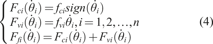
In general, using a symbolic function directly in the Coulomb friction model results in discontinuous and nonsmooth functions in the dynamics model, which affects the performance of the controller. Here the sign function can be replaced by the hyperbolic tangent function, thus ensuring its continuous and smooth properties.

s i g n (\dot{θ_{i}}) \approx \tanh (δ \dot{θ_{i}}), i = 1,2, \dots, n

(5)

where δ is chosen large enough to approximate the sign function more precisely.

There are modeling errors and unmodeled parts of the robotic arm system dynamics model. These can be considered uncertainties. Equation (3) can be rewritten as

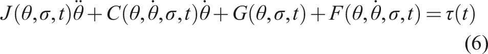
J (θ, σ, t) \ddot{θ} + C (θ, \dot{θ}, σ, t) \dot{θ} + G (θ, σ, t) + F (θ, \dot{θ}, σ, t) = τ (t)

(6)

Uncertainty in equation (6) is denoted by the parameter σ ∈ Rⁿ. Suppose the uncertainty in the robotic arm system is time-varying but bounded, and there exists a known set sum ⊂ Rⁿ that satisfies σ ∈ ∑ ⊂ Rⁿ holds.

The system matrix of the above dynamics model (equation (6)) has the following properties (Yang et al., 2018):

Property 1

For all θ, J(θ, σ, t) > 0 is symmetric and uniformly bounded. That is

0 < ζ_{\min} E \leq J (θ, σ, t) \leq ζ_{\max} E

(7)

with E is the identity matrix, ζ_min and ζ_max are positive scalars which can be obtained from any given robot.

Property 2

For all θ and $\dot{θ}$ , satisfying

S (θ, \dot{θ}, σ, t) = \dot{J} (θ, σ, t) - 2 C (θ, \dot{θ}, σ, t)

(8)

where

S (θ, \dot{θ}, σ, t)

is skew symmetric, and

\dot{J} (θ, σ, t)

is the derivative of J (θ, σ, t) for time. Then, we have

ξ^{T} S (θ, \dot{θ}, σ, t) ξ = 0

, for any ξ ∈ Rⁿ.

3. Controller design and stability proof

3.1. Controller design

The controller design of a mechanical system needs to ensure excellent performance (accuracy, stability, speed, and robustness) of the motion of the controlled object. The proposed controller enables each joint to track the given trajectory with the desired dynamic quality for a n-DOF robotic arm.

The desired tracking trajectory θ^d(t) ∈ Rⁿ, t ∈ [t₀, t₁] for a n-DOF robotic arm system, thus ${\dot{θ}}^{d} (t)$ and ${\overset{. .}{θ}}^{d} (t)$ are the the desired velocity and acceleration, respectively. For all t ∈ [t₀, ∞] → Rⁿ, assuming that θ^d(t) is C², and θ^d(t), ${\dot{θ}}^{d} (t)$ and ${\overset{. .}{θ}}^{d} (t)$ are uniformly bounded and uniformly ultimately bounded. Actual position, velocity, and acceleration of the robotic arm joints are described by θ(t), $\dot{θ} (t)$ , and $\overset{. .}{θ} (t)$ , respectively. So we can get the tracking error

e (t) = θ (t) - θ^{d} (t)

(9)

and the trajectory tracking error vector can be defined as

\bar{e} (t) : = [\begin{array}{l} e (t) \\ \dot{e} (t) \end{array}]

(10)

where

\dot{e} (t) = \dot{θ} (t) - {\dot{θ}}^{d} (t)

According to equation (9), equation (6) can be rewritten as

\begin{array}{l} τ (t) = J (θ^{d} + e, σ, t) ({\overset{. .}{θ}}^{d} + \ddot{e}) \\ + C (θ^{d} + e, {\dot{θ}}^{d} + \dot{e}, σ, t) ({\dot{θ}}^{d} + \dot{e}) \\ + G (θ^{d} + e, σ, t) + F (θ^{d} + e, {\dot{θ}}^{d} + \dot{e}, σ, t) \end{array}

(11)

where

\ddot{e} (t) = \ddot{θ} (t) - {\ddot{θ}}^{d} (t)

The internal uncertainty of the system is mainly caused by the system matrix model error in the dynamic model, where the uncertainties in J (⋅), C (⋅), G (⋅), and F (⋅) are separated out as

{\begin{cases} J (θ^{d} + e, σ, t) = \tilde{J} (θ^{d} + e, t) + Δ J (θ^{d} + e, σ, t) \\ C (θ^{d} + e, {\dot{θ}}^{d} + \dot{e}, σ, t) = \tilde{C} (θ^{d} + e, {\dot{θ}}^{d} + \dot{e}, t) \\ + Δ C (θ^{d} + e, {\dot{θ}}^{d} + \dot{e}, σ, t) \\ G (θ^{d} + e, σ, t) = \tilde{G} (θ^{d} + e, t) + Δ G (θ^{d} + e, σ, t) \\ F (θ^{d} + e, {\dot{θ}}^{d} + \dot{e}, σ, t) = \tilde{F} (θ^{d} + e, {\dot{θ}}^{d} + \dot{e}, t) + \\ + Δ F (θ^{d} + e, {\dot{θ}}^{d} + \dot{e}, σ, t) \end{cases}

(12)

where

\tilde{(\cdot)}

is the nominal item, Δ(⋅) is uncertain term connected to σ.

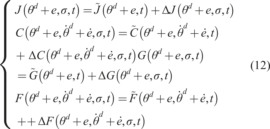
In general, using the nominal terms $\tilde{J} (\cdot)$ , $\tilde{C} (\cdot)$ , $\tilde{G} (\cdot)$ , and $\tilde{F} (\cdot)$ to estimate the parameters of the actual system can minimize the uncertainty induced by the system parameters. We assume that the uncertainty is bounded. Based on the uncertainty boundary. Such that

ρ (e, \dot{e}, σ, t) ⩾ ‖ Φ (e, \dot{e}, σ, t) ‖

(13)

where

ρ (e, \dot{e}, σ, t)

is the upper bound of the combined effect of all uncertainties.

‖ \cdot ‖

represents the Euclidean norm, which can also be written as

{‖ \cdot ‖}_{2}

. And

\begin{array}{l} Φ (e, \dot{e}, σ, t) = - Δ J (θ^{d} + e, σ, t) ({\overset{. .}{θ}}^{d} - S \dot{e}) \\ - Δ C (θ^{d} + e, {\dot{θ}}^{d} + \dot{e}, σ, t) ({\dot{θ}}^{d} - S e) \\ - Δ G (θ^{d} + e, σ, t) \\ - Δ F (θ^{d} + e, {\dot{θ}}^{d} + \dot{e}, σ, t) \end{array}

(14)

where

S = d i a g {{[s_{i}]}_{n \times n}}, s_{i} > 0, i = 1,2, \dots, n

(15)

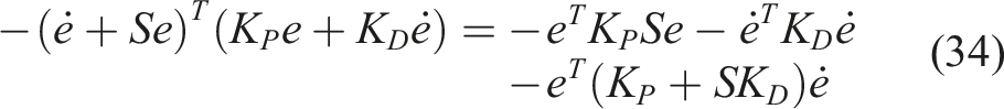
When all uncertainties are ignored, that is $J (\cdot) = \tilde{J} (\cdot)$ , $C (\cdot) = \tilde{C} (\cdot)$ , $G (\cdot) = \tilde{G} (\cdot)$ , $F (\cdot) = \tilde{F} (\cdot)$ . Then, $Φ (e, \dot{e}, σ, t) \equiv 0$ .

The designed controller guarantees that the trajectory tracking error remains within the set boundary. The approach to ensure given performance limitations may be found in Ref. Chen (1986). The deterministic robust control technique described in this work may be written as

\begin{array}{l} τ (t) = & \tilde{J} (θ^{d} + e, t) ({\overset{. .}{θ}}^{d} - S \dot{e}) + \tilde{C} (θ^{d} + e, {\dot{θ}}^{d} + \dot{e}, t) ({\dot{θ}}^{d} - S e) \\ + \tilde{G} (θ^{d} + e, t) + \tilde{F} (θ^{d} + e, {\dot{θ}}^{d} + \dot{e}, t) - K_{P} e - K_{D} \dot{e} \\ - \frac{φ}{χ + γ} \end{array}

(16)

where

K_{P} = d i a g {{[k_{p i}]}_{n \times n}}, k_{p i} > 0, i = 1,2, \dots, n

(17)

is the proportional coefficient. And

K_{D} = d i a g {{[k_{d i}]}_{n \times n}}, k_{d i} > 0, i = 1,2, \dots, n

(18)

is the differential coefficient. And φ and χ can be described as

φ = α^{2} (\dot{e} + S e) ρ^{4} {‖ \dot{e} + S e ‖}^{2}

(19)

χ = α {‖ \dot{e} + S e ‖}^{2} ρ^{2}

(20)

where α and γ represent positive design parameters determined from specific engineering examples. Theoretically, the proposed controller (equation (16)) can ensure that the ultimate boundedness sphere of the system tracking error

\bar{e} (t)

is small enough by selecting the appropriate γ and α design parameters, which can be seen in the parameters selection section for a detailed description.

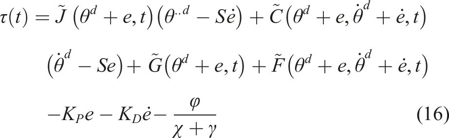
Based on the proposed controller structure shown in Figure 1, the first part of the controller is a nominal system. The last item is the compensation for system uncertainty, reducing the impact of uncertainty on the system. The controller (equation (16)) consists of the model- and error-based PD control (non-error-based conventional PD control) and robust term.

Figure 1.

The structural block diagram of the proposed robust controller.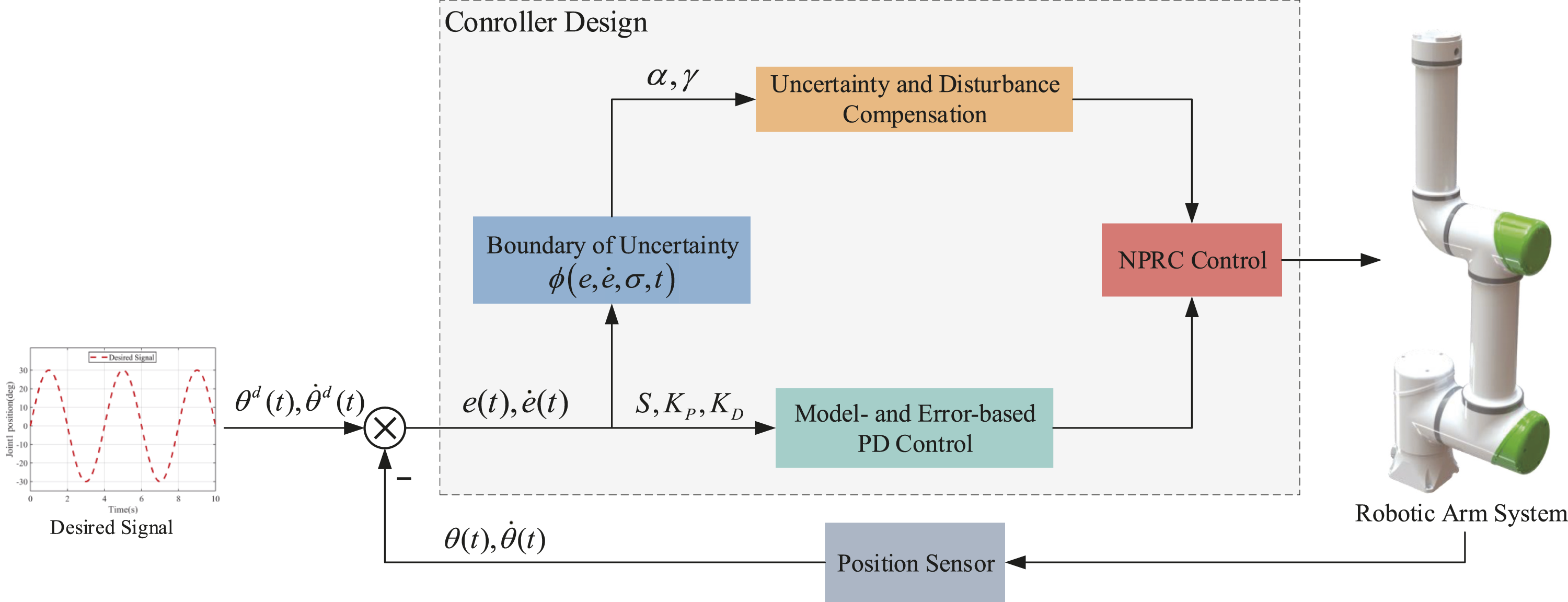

3.2. Proof of stability

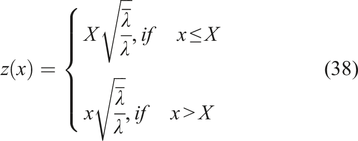
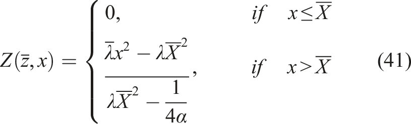
Applying the suggested controller equation (16) to the planted object system (equation (6)) must prove that the trajectory tracking error $\bar{e} (t)$ is uniformly bounded and uniformly ultimately bounded. The ultimate boundedness ball can be made small enough by selecting the proper parameter γ, α, and ρ. The properties can be described explicitly as

1) Uniform boundedness: There exists a z(x) < ∞ such that ‖θ(t)‖ ≤ z(x) for any x > 0 with ‖θ(t₀)‖ ≤ x, ∀t ≥ t₀.

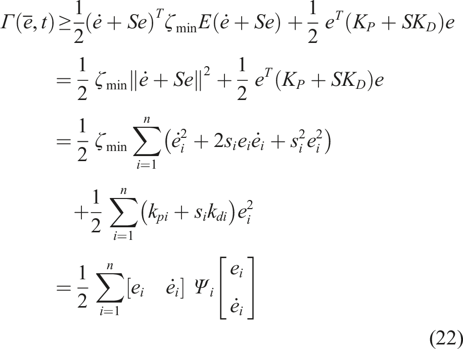
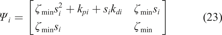
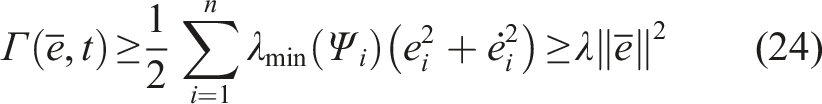
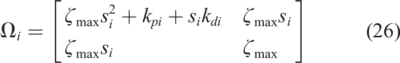
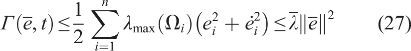
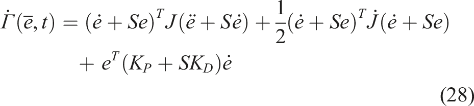
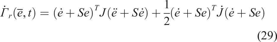
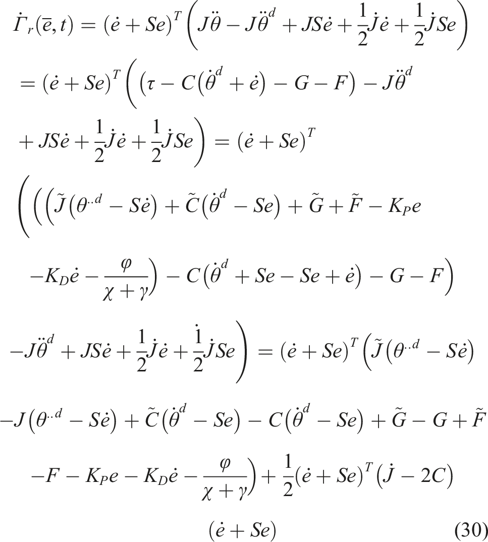
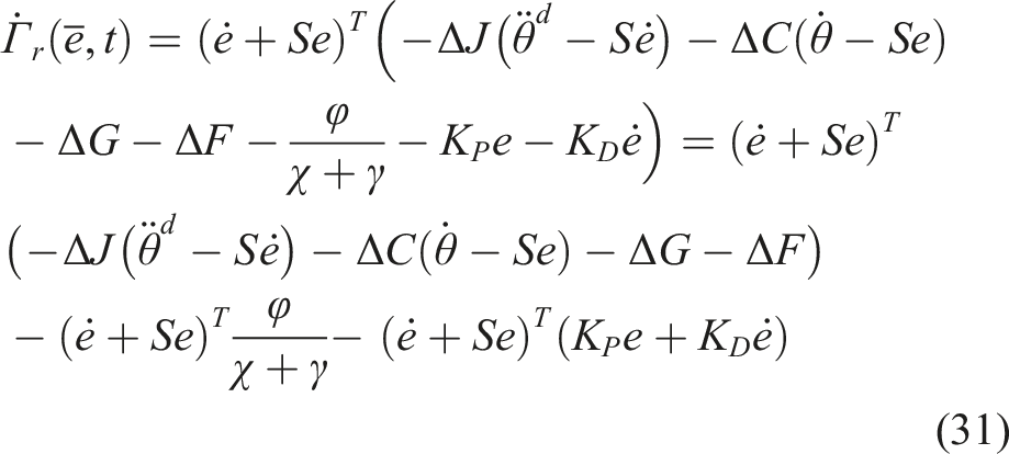
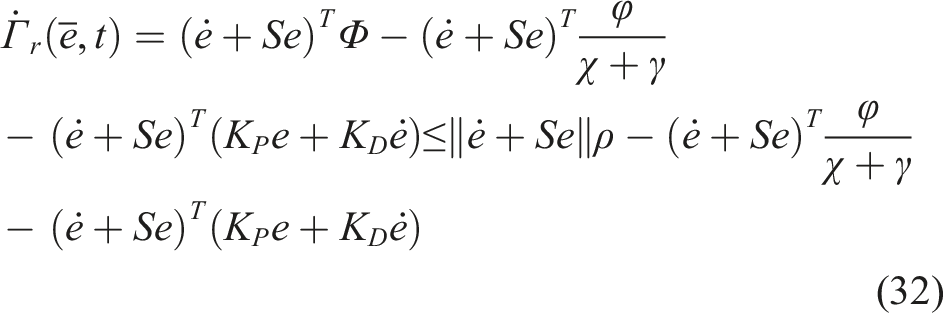
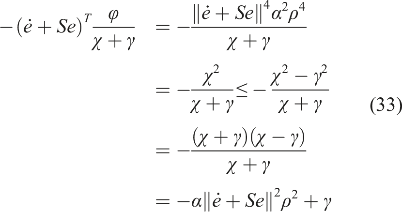
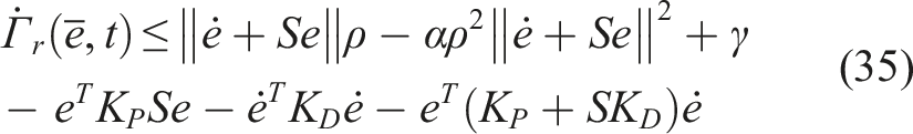
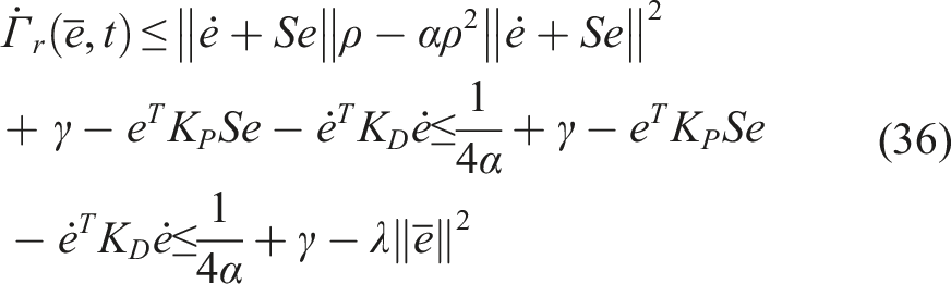
2) Uniform ultimate boundedness: For any x > 0 with ‖θ(t₀)‖ ≤ x, there exists a $\underline{z} > 0$ , such that $‖ θ (t) ‖ \geq \bar{z}$ for all $\bar{z} > \underline{z}$ as $t \geq t_{0} + Z (\bar{z}, x)$ , and $Z (\bar{z}, x) < \infty$ .

Proof

The stability of the equilibrium state is determined by selecting the Lyapunov candidate energy function and examining whether the function decays with time. Firstly, we choose a Lyapunov function candidate and verify that it is valid (positive definite and decrescent). The candidate function is selected as

Γ (\bar{e}, t) = \frac{1}{2} {(\dot{e} + S e)}^{T} J (\dot{e} + S e) + \frac{1}{2} e^{T} (K_{P} + S K_{D}) e

(21)

According to Property 1, J (θ, σ, t) is bounded. Substituting the Inequality (7) into equation (21), we get

\begin{array}{l} Γ (\bar{e}, t) \geq \frac{1}{2} {(\dot{e} + S e)}^{T} ζ_{\min} E (\dot{e} + S e) + \frac{1}{2} e^{T} (K_{P} + S K_{D}) e \\ = \frac{1}{2} ζ_{\min} {‖ \dot{e} + S e ‖}^{2} + \frac{1}{2} e^{T} (K_{P} + S K_{D}) e \\ = \frac{1}{2} ζ_{\min} \sum_{i = 1}^{n} ({\dot{e}}_{i}^{2} + 2 s_{i} e_{i} {\dot{e}}_{i} + s_{i}^{2} e_{i}^{2}) \\ + \frac{1}{2} \sum_{i = 1}^{n} (k_{p i} + s_{i} k_{d i}) e_{i}^{2} \\ = \frac{1}{2} \sum_{i = 1}^{n} [e_{i} {\dot{e}}_{i}] Ψ_{i} [\begin{array}{l} e_{i} \\ {\dot{e}}_{i} \end{array}] \end{array}

(22)

where

Ψ_{i} = [\begin{array}{l} ζ_{\min} s_{i}^{2} + k_{p i} + s_{i} k_{d i} & ζ_{\min} s_{i} \\ ζ_{\min} s_{i} & ζ_{\min} \end{array}]

(23)

Obviously, matrix Ψ_i > 0, ∀i. Thus $Γ (\bar{e}, t)$ is positive definite by the following inequlity (Rayleigh theorem (Noble and Daniel, 1977)

Γ (\bar{e}, t) \geq \frac{1}{2} \sum_{i = 1}^{n} λ_{\min} (Ψ_{i}) (e_{i}^{2} + {\dot{e}}_{i}^{2}) \geq \underline{λ} {‖ \bar{e} ‖}^{2}

(24)

where

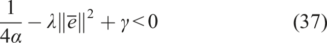
\underline{λ} = 1 / 2 \min {λ_{\min} (Ψ_{1}), λ_{\min} (Ψ_{2}), \dots, λ_{\min} (Ψ_{n})} > 0

Similarly, according to the upper bound of J (θ, σ, t), there is

\begin{array}{l} Γ (\bar{e}, t) \leq & \frac{1}{2} {(\dot{e} + S e)}^{T} ζ_{\max} E (\dot{e} + S e) + \frac{1}{2} e^{T} (K_{P} + S K_{D}) e \\ = & \frac{1}{2} \sum_{i = 1}^{n} [e_{i} {\dot{e}}_{i}] Ω_{i} [\begin{array}{l} e_{i} \\ {\dot{e}}_{i} \end{array}] \end{array}

(25)

where

Ω_{i} = [\begin{array}{l} ζ_{\max} s_{i}^{2} + k_{p i} + s_{i} k_{d i} & ζ_{\max} s_{i} \\ ζ_{\max} s_{i} & ζ_{\max} \end{array}]

(26)

That is

Γ (\bar{e}, t) \leq \frac{1}{2} \sum_{i = 1}^{n} λ_{\max} (Ω_{i}) (e_{i}^{2} + {\dot{e}}_{i}^{2}) \leq \bar{λ} {‖ \bar{e} ‖}^{2}

(27)

where

\bar{λ} = 1 / 2 \max {λ_{\max} (Ω_{1}), λ_{\max} (Ω_{2}), \dots, λ_{\max} (Ω_{n})} > 0

Combine Inequalities (24) and (27), we can get $\underline{λ} ‖ \bar{e} ‖^{2} \leq Γ (\bar{e}, t) \leq \bar{λ} ‖ \bar{e} ‖^{2}$ . Subsequently, the stability of the system can be further verified by deriving the time t from $Γ (\bar{e}, t)$ .

\begin{array}{l} \dot{Γ} (\bar{e}, t) & = {(\dot{e} + S e)}^{T} J (\ddot{e} + S \dot{e}) + \frac{1}{2} {(\dot{e} + S e)}^{T} \dot{J} (\dot{e} + S e) \\ + e^{T} (K_{P} + S K_{D}) \dot{e} \end{array}

(28)

Let

{\dot{Γ}}_{r} (\bar{e}, t) = {(\dot{e} + S e)}^{T} J (\ddot{e} + S \dot{e}) + \frac{1}{2} {(\dot{e} + S e)}^{T} \dot{J} (\dot{e} + S e)

(29)

Further, substituting $\dot{e} (t)$ , $\ddot{e} (t)$ , equation (3) and equation (16) into equation (29). ${\dot{Γ}}_{r} (\bar{e}, t)$ can be specified as

\begin{array}{l} {\dot{Γ}}_{r} (\bar{e}, t) = {(\dot{e} + S e)}^{T} (J \ddot{θ} - J {\ddot{θ}}^{d} + J S \dot{e} + \frac{1}{2} \dot{J} \dot{e} + \frac{1}{2} \dot{J} S e) \\ = {(\dot{e} + S e)}^{T} ((τ - C ({\dot{θ}}^{d} + \dot{e}) - G - F) - J {\ddot{θ}}^{d} + J S \dot{e} + \frac{1}{2} \dot{J} \dot{e} + \frac{1}{2} \dot{J} S e) \\ = {(\dot{e} + S e)}^{T} (((\tilde{J} ({\overset{. .}{θ}}^{d} - S \dot{e}) + \tilde{C} ({\dot{θ}}^{d} - S e) + \tilde{G} + \tilde{F} - K_{P} e - K_{D} \dot{e} - \frac{φ}{χ + γ}) - C ({\dot{θ}}^{d} + S e - S e + \dot{e}) - G - F) - J {\ddot{θ}}^{d} + J S \dot{e} + \frac{1}{2} \dot{J} \dot{\dot{e} + \frac{1}{2} \dot{J} S e}) \\ = {(\dot{e} + S e)}^{T} (\tilde{J} ({\overset{. .}{θ}}^{d} - S \dot{e}) - J ({\overset{. .}{θ}}^{d} - S \dot{e}) + \tilde{C} ({\dot{θ}}^{d} - S e) - C ({\dot{θ}}^{d} - S e) + \tilde{G} - G + \tilde{F} - F - K_{P} e - K_{D} \dot{e} - \frac{φ}{χ + γ}) \\ + \frac{1}{2} {(\dot{e} + S e)}^{T} (\dot{J} - 2 C) (\dot{e} + S e) \end{array}

(30)

With Property 2 and equation (12), ${\dot{Γ}}_{r} (\bar{e}, t)$ can be rephrased as

\begin{array}{l} {\dot{Γ}}_{r} (\bar{e}, t) = {(\dot{e} + S e)}^{T} (- Δ J ({\ddot{θ}}^{d} - S \dot{e}) - Δ C (\dot{θ} - S e) - Δ G - Δ F - \frac{φ}{χ + γ} - K_{P} e - K_{D} \dot{e}) \\ = {(\dot{e} + S e)}^{T} (- Δ J ({\ddot{θ}}^{d} - S \dot{e}) - Δ C (\dot{θ} - S e) - Δ G - Δ F) - {(\dot{e} + S e)}^{T} \frac{φ}{χ + γ} \\ - {(\dot{e} + S e)}^{T} (K_{P} e + K_{D} \dot{e}) \end{array}

(31)

By equation (14), there is

\begin{array}{l} {\dot{Γ}}_{r} (\bar{e}, t) = {(\dot{e} + S e)}^{T} Φ - {(\dot{e} + S e)}^{T} \frac{φ}{χ + γ} \\ - {(\dot{e} + S e)}^{T} (K_{P} e + K_{D} \dot{e}) \\ \leq ‖ \dot{e} + S e ‖ ρ - {(\dot{e} + S e)}^{T} \frac{φ}{χ + γ} \\ - {(\dot{e} + S e)}^{T} (K_{P} e + K_{D} \dot{e}) \end{array}

(32)

According to equation (19) and equation (20)

\begin{array}{l} - {(\dot{e} + S e)}^{T} \frac{φ}{χ + γ} & = - \frac{{‖ \dot{e} + S e ‖}^{4} α^{2} ρ^{4}}{χ + γ} \\ = - \frac{χ^{2}}{χ + γ} \leq - \frac{χ^{2} - γ^{2}}{χ + γ} \\ = - \frac{(χ + γ) (χ - γ)}{χ + γ} \\ = - α {‖ \dot{e} + S e ‖}^{2} ρ^{2} + γ \end{array}

(33)

and

\begin{array}{l} - {(\dot{e} + S e)}^{T} (K_{P} e + K_{D} \dot{e}) = & - e^{T} K_{P} S e - {\dot{e}}^{T} K_{D} \dot{e} \\ - e^{T} (K_{P} + S K_{D}) \dot{e} \end{array}

(34)

Combine Inequalities (32), (33), and equation (34), ${\dot{Γ}}_{r} (\bar{e}, t)$ can be rewritten as

\begin{array}{l} {\dot{Γ}}_{r} (\bar{e}, t) \leq & {‖ \dot{e} + S e ‖ ρ - α ρ^{2} ‖ \dot{e} + S e ‖}^{2} + γ \\ - e^{T} K_{P} S e - {\dot{e}}^{T} K_{D} \dot{e} - e^{T} (K_{P} + S K_{D}) \dot{e} \end{array}

(35)

Substituting Inequality (35) into equation (28), there is

\begin{array}{l} {\dot{Γ}}_{r} (\bar{e}, t) \leq {‖ \dot{e} + S e ‖ ρ - α ρ^{2} ‖ \dot{e} + S e ‖}^{2} \\ + γ - e^{T} K_{P} S e - {\dot{e}}^{T} K_{D} \dot{e} \\ \leq \frac{1}{4 α} + γ - e^{T} K_{P} S e - {\dot{e}}^{T} K_{D} \dot{e} \\ \leq \frac{1}{4 α} + γ - λ {‖ \bar{e} ‖}^{2} \end{array}

(36)

where λ = min

{λ_{\min} (K_{P} S), λ_{\min} (K_{D})}

For all $‖ \bar{e} (t) ‖$ , it shows that $\dot{Γ} (\bar{e}, t)$ is negative definite, there is

\frac{1}{4 α} - λ {‖ \bar{e} ‖}^{2} + γ < 0

(37)

where α, λ and γ are all determined, so

\dot{Γ} (\bar{e}, t)

is negative when

‖ \bar{e} (t) ‖

is large enough.

Consequently, the controller (equation (16)) can assure the uniform boundedness and uniform ultimate boundedness of the robotic arm system (equation (6)). First is the uniform boundedness, for any x > 0 with $‖ \bar{e} (t_{0}) ‖ > 0$ , we can get

z (x) = {\begin{cases} X \sqrt{\frac{\bar{λ}}{\underline{λ}}}, i f x \leq X \\ x \sqrt{\frac{\bar{λ}}{\underline{λ}}}, i f x > X \end{cases}

(38)

where

X = \sqrt{\frac{1}{4 α x}}

(39)

such that

‖ \bar{e} (t) ‖ \leq z (x)

for all t ≥ t₀.

Second is uniform ultimate boundedness, for any $\bar{z}$ with

\bar{z} > X \sqrt{\frac{\bar{λ}}{\underline{λ}}}

(40)

the performance can be guaranteed by

Z (\bar{z}, x) = {\begin{cases} 0, & i f x \leq \bar{X} \\ \frac{\bar{λ} x^{2} - \underline{λ} {\bar{X}}^{2}}{λ {\bar{X}}^{2} - \frac{1}{4 α}}, i f x > \bar{X} \end{cases}

(41)

and

\bar{X} = \bar{z} \sqrt{\frac{\underline{λ}}{\bar{λ}}}

(42)

Such that $‖ \bar{e} (t) ‖ \leq \bar{z}$ , $\forall t \geq t_{0} + Z (\bar{z}, x)$ (Corless and Leitmann, 1981).

4. Numerical simulation and experimental validation

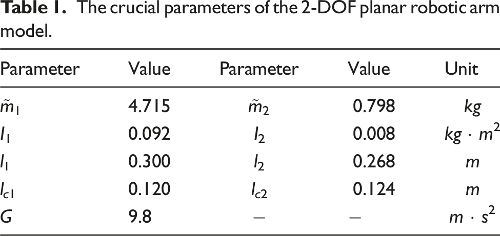
Based on the control scheme (equation (16)) proposed above, numerical simulation and experimental verification on the controlled object 2-DOF planar robotic arm are performed in this section. Figure 2 illustrates a simplified 2-DOF planar robotic arm model. Where m₁ and m₂ are masses of the first arm and the second arm, θ₁ and θ₂ are the positive rotation angles of joints 1 and 2, l₁ and l₂ are the lengths of the two arms, respectively. Points C₁ and C₂ are the centroid of the first arm and the second arm. l_c1 is the distance of the point C₁ to the origin point O₁, and l_c2 is the distance of the point C₂ to the origin point O₂.

Figure 2.

The schematic representation of the simplified 2-DOF planar robotic arm.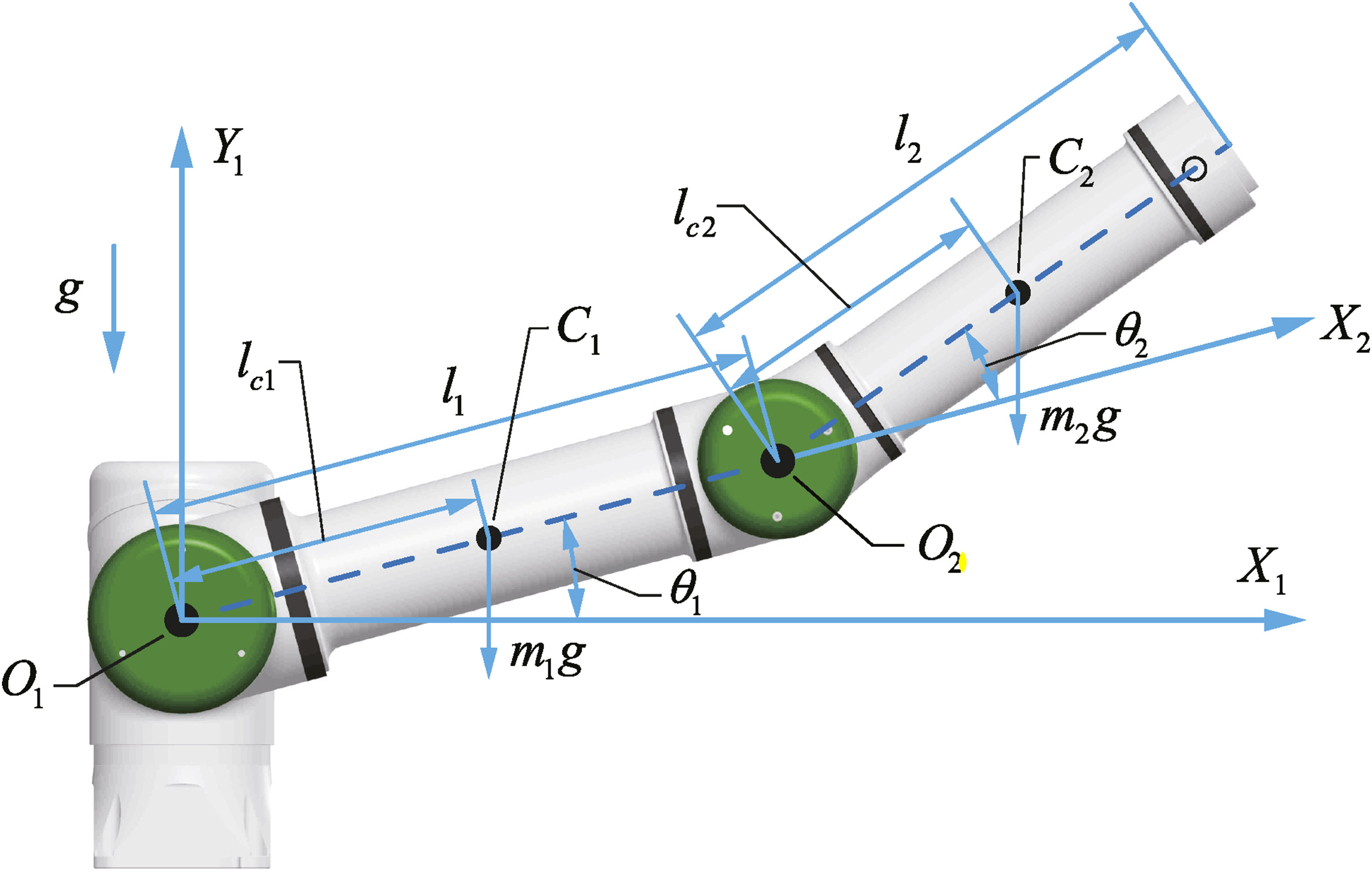

The comparison with other control algorithms can better demonstrate the superiority of the proposed control algorithm. In addition to the proposed novel practical robust control (NPRC), the comparison control algorithms include classical PID control and model- and error-based PD control (MEBPD). Considering the relative fairness, the simulation and experiments are repeated several times for each control algorithm in the same environment, and the optimal performance of each control algorithm is selected for comparison.

4.1. Parameters selection

Analyze and determine the relevant parameters for each algorithm at the optimal performance, as detailed below.

The nominal parameter matrix of the system in equation (16) does not vary depending on the control algorithm, and according to the general dynamics model (equation (3)) of the 2-DOF planar robotic arm, they can be written as

\tilde{J} = [\begin{array}{l} j_{1} + 2 j_{3} \cos θ_{2} & j_{2} + j_{3} \cos θ_{2} \\ j_{2} + j_{3} \cos θ_{2} & j_{2} \end{array}]

(43)

\tilde{C} = j_{3} \sin θ_{2} [\begin{array}{l} - {\dot{θ}}_{2} & - {\dot{θ}}_{1} - {\dot{θ}}_{2} \\ {\dot{θ}}_{1} & 0 \end{array}]

(44)

\tilde{G} = [\begin{array}{l} g_{1} \cos θ_{1} + g_{2} \cos (θ_{1} + θ_{2}) \\ g_{2} \cos (θ_{1} + θ_{2}) \end{array}]

(45)

where

{\begin{cases} j_{1} = {\tilde{m}}_{1} l_{c 1}^{2} + {\tilde{m}}_{2} (l_{1}^{2} + l_{c 2}^{2}) + I_{1} + I_{2} \\ j_{2} = {\tilde{m}}_{2} l_{c 2}^{2} + I_{2} \\ j_{3} = {\tilde{m}}_{2} l_{1} l_{c 2} \\ g_{1} = {\tilde{m}}_{1} l_{c 1} g + {\tilde{m}}_{2} l_{1} g \\ g_{2} = {\tilde{m}}_{2} l_{c 2} g \end{cases}

(46)

and I_i, i = 1, 2, is the ith moment of inertia of the ith link. Table 1 contains the specific parameters of the system model here were obtained through industrial CAD software.

Table 1.

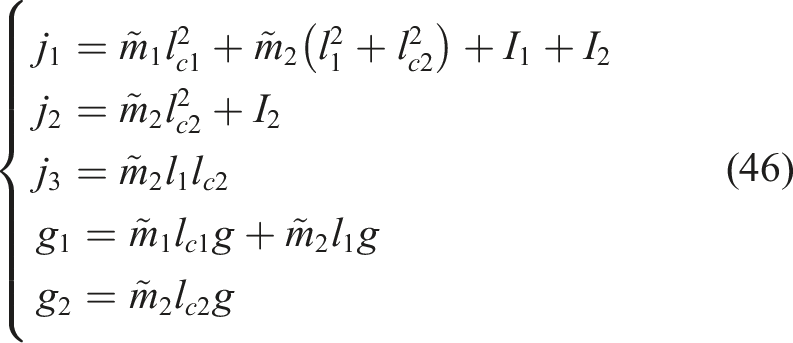
The crucial parameters of the 2-DOF planar robotic arm model.

Parameter	Value	Parameter	Value	Unit
${\tilde{m}}_{1}$	4.715	${\tilde{m}}_{2}$	0.798	kg
I ₁	0.092	I ₂	0.008	kg ⋅ m²
l ₁	0.300	l ₂	0.268	m
l _c1	0.120	l _c2	0.124	m
G	9.8	−	−	m ⋅ s²

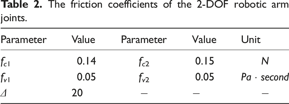
Further determine the parameters in the frictional forces to which the system is subjected. Similarly, according to the friction model in equation (4), we can get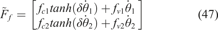

{\tilde{F}}_{f} = [\begin{array}{l} f_{c 1} \tanh (δ {\dot{θ}}_{1}) + f_{v 1} {\dot{θ}}_{1} \\ f_{c 2} \tanh (δ {\dot{θ}}_{2}) + f_{v 2} {\dot{θ}}_{2} \end{array}]

(47)

The friction coefficients of the 2-DOF arm joints are shown in Table 2, which more accurately reflects the actual friction.

Table 2.

The friction coefficients of the 2-DOF robotic arm joints.

Parameter	Value	Parameter	Value	Unit
f _c1	0.14	f _c2	0.15	N
f _v1	0.05	f _v2	0.05	Pa ⋅ second
Δ	20	−	−	−

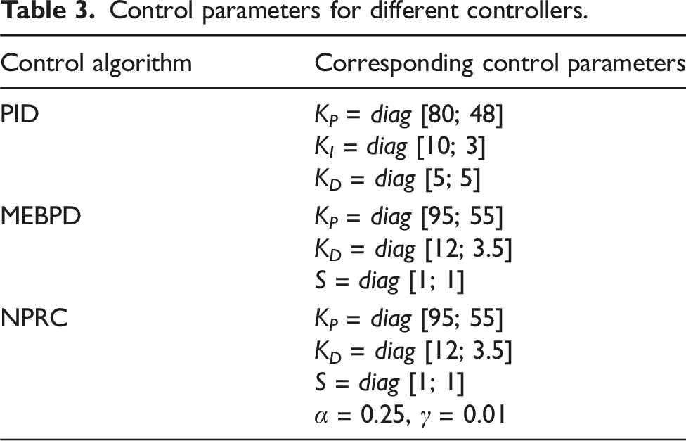
In addition, the proper selection of parameters in the control algorithm can enhance the performance of the controller and reduce the control cost.

Among them, the diagonal matrix S directly affects the convergence rate of $\bar{e} (t)$ . The choice of the diagonal elements of matrix S requires a balance between the convergence speed and the control cost. In the simulations and experiments, matrix S is selected as an identity matrix, which is to reflect the simplicity and ease of implementation of the proposed control structure and better to distinguish the influence of other essential parameters on the controller. The proportional parameter K_P may cause overshoot and oscillation of the system while increasing the system response speed and decreasing the steady-state error. The response speed and overshoot of the system can be reduced by adjusting the differential parameter K_D, but it will increase the steady-state error. By choosing appropriate parameters γ and α, the ultimately bounded ball of the trajectory tracking error $\bar{e} (t)$ may be kept small enough. Specifically, according to equation (36), we let

\frac{1}{4 α} + γ - λ {‖ \bar{e} ‖}^{2} = 0

(48)

and from it, there is

‖ \bar{e} ‖ = \sqrt{\frac{1}{4 α λ} + \frac{γ}{λ}}

(49)

where λ = min

{λ_{\min} (K_{P} S), λ_{\min} (K_{D})}

. That is, when K_P, K_D, and S are forced to be determined to meet other performance metrics, the size of

‖ \bar{e} (t) ‖

is only relevant to α and γ.

Through repeatedly testing different control algorithms (PID, MEBPD, and NPRC) in the same environment, we finally selected the parameters for the relative optimal performance of each control algorithm as shown in Table 3.

Table 3.

Control parameters for different controllers.

Control algorithm	Corresponding control parameters
PID	K_P = diag [80; 48]
	K_I = diag [10; 3]
	K_D = diag [5; 5]
MEBPD	K_P = diag [95; 55]
	K_D = diag [12; 3.5]
	S = diag [1; 1]
NPRC	K_P = diag [95; 55]
	K_D = diag [12; 3.5]
	S = diag [1; 1]
	α = 0.25, γ = 0.01

4.2. Numerical simulation results

The introduction of the reference step signal and the sine signal can compare the transient performance, steady-state performance, and trajectory tracking performance of each control algorithm more comprehensively. The step signal is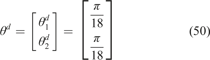

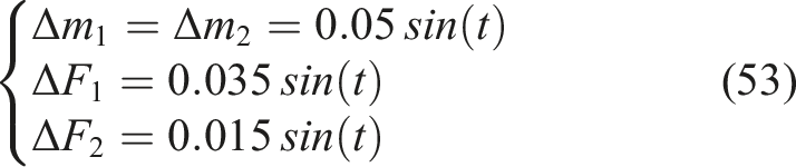
θ^{d} = [\begin{array}{l} θ_{1}^{d} \\ θ_{2}^{d} \end{array}] = [\begin{array}{l} \frac{π}{18} \\ \frac{π}{18} \end{array}]

(50)

and the sinusoidal signal is

θ^{d} = [\begin{array}{l} θ_{1}^{d} \\ θ_{2}^{d} \end{array}] = [\begin{array}{l} \frac{π}{6} \sin \frac{π}{2} t \\ \frac{π}{6} \sin \frac{π}{2} t \end{array}]

(51)

In practical engineering, the precise model of the research object is difficult to obtain. Therefore, we introduce uncertainties Δm₁, Δm₁, ΔF₁, and ΔF₂ (which are bounded) in the MEBPD control algorithm and NPRC control algorithm to better compare the robust performance of each control algorithm. The uncertainties are assumed as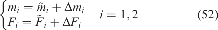

{\begin{cases} m_{i} = {\tilde{m}}_{i} + Δ m_{i} \\ F_{i} = {\tilde{F}}_{i} + Δ F_{i} \end{cases} i = 1,2

(52)

where

{\begin{cases} Δ m_{1} = Δ m_{2} = 0.05 \sin (t) \\ Δ F_{1} = 0.035 \sin (t) \\ Δ F_{2} = 0.015 \sin (t) \end{cases}

(53)

In the sinusoidal signal trajectory tracking, we set an initial error. Otherwise, the trajectory tracking state can be observed more distinctly. Moreover, the robust performance of each control algorithm can be verified. The initial error can be described as

e (t) = [\begin{array}{l} \frac{π}{18} \\ \frac{π}{18} \end{array}]

(54)

and

\dot{e} (t) = [\begin{array}{l} 0 \\ 0 \end{array}]

(55)

The simulation results are as follows:

4.2.1. Step response

Figure 3(a) and (b) illustrate the step response simulation results of the 2-DOF planar robotic arm system under the different control schemes. The simulation results of joint 1 are used as an example to analyze and compare each of the three control algorithms. Regarding terms of response speed, NPRC took about 0.172 s to reach the steady-state, and PID and MEBPD took about 0.672 s and 0.354 s, respectively. And the steady-state error range for the NPRC algorithm was approximately e₁ = −3.077 × 10⁻⁵ ∼ 3.073 × 10⁻⁵ deg, and the steady-state error ranges for PID and MEBPD were approximately e₁ = −2.269 × 10⁻⁴ ∼ − 1.274 × 10⁻⁴ deg and e₁ = −1.139 × 10⁻⁴ ∼ 1.143 × 10⁻⁴ deg, respectively. Similarly, for joint 2, the NPRC took about 0.131 s to reach a steady-state, and the PID and MEBPD took about 0.519 s and 0.311 s, respectively. The steady-state error range for NPRC was approximately e₂ = −1.554 × 10⁻⁵ ∼ 1.562 × 10⁻⁵ deg, and for PID and MEBPD was approximately e₂ = −1.555 × 10⁻⁴ ∼ − 6.395 × 10⁻⁵ deg and e₂ = −5.690 × 10⁻⁴ ∼ 5.688 × 10⁻⁴ deg, respectively. The above analysis indicated that the NPRC control algorithm has a faster response and a smaller error range than the other two control algorithms for both joints 1 and 2.

Figure 3.

The position step response simulation curves of the two joints of the 2-DOF planar robotic arm.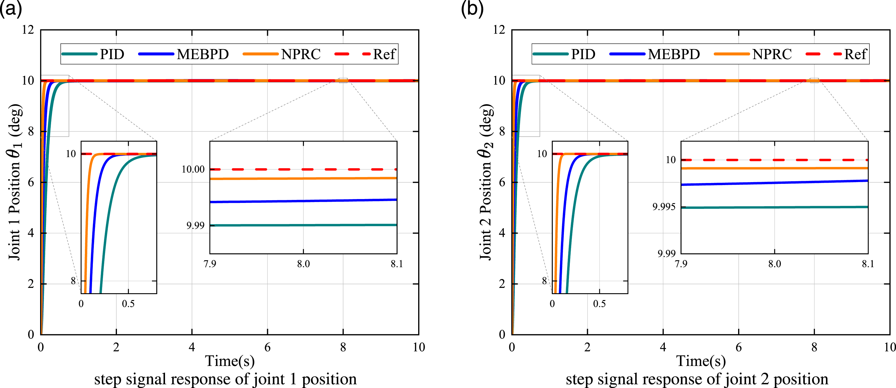

4.2.2. Sinusoidal signal tracking

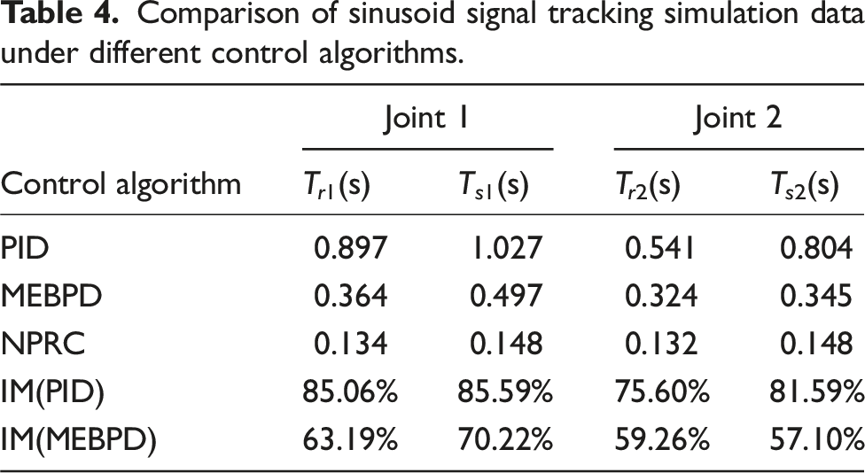
Figures 4(a)–5(b) show the simulation results of sine signal trajectory tracking for the three control algorithms. The NPRC control algorithm is the first to catch up with the sinusoidal signal for a given initial error as indicated in Figures 4(a) and 5(a). It can maintain a small tracking error to track the desired trajectory as shown in Figures 4(b) and 5(b). Specifically, the NPRC control algorithm has tracking errors of e₁ = −0.0045 ∼ 0.0041 deg, e₂ = −0.0017 ∼ 0.0014 deg, while the PID and MEBPD control algorithms have tracking errors of e₁ = −0.1106 ∼ 0.0876 deg, e₂ = −0.1205 ∼ 0.1120 deg, and e₁ = −0.0113 ∼ 0.0104 deg, e₂ = −0.0.0063 ∼ 0.0054 deg, respectively. The above indicates that the NPRC control algorithm reaches up to the desired trajectory faster and maintains a minor tracking error than the other control algorithms, whether joint 1 or joint 2.

Figure 4.

The sinusoidal signal trajectory tracking simulation curves of the joint 1 of the 2-DOF planar robotic arm.

Figure 5.

The sinusoidal signal trajectory tracking simulation curves of the joint 2 of the 2-DOF planar robotic arm.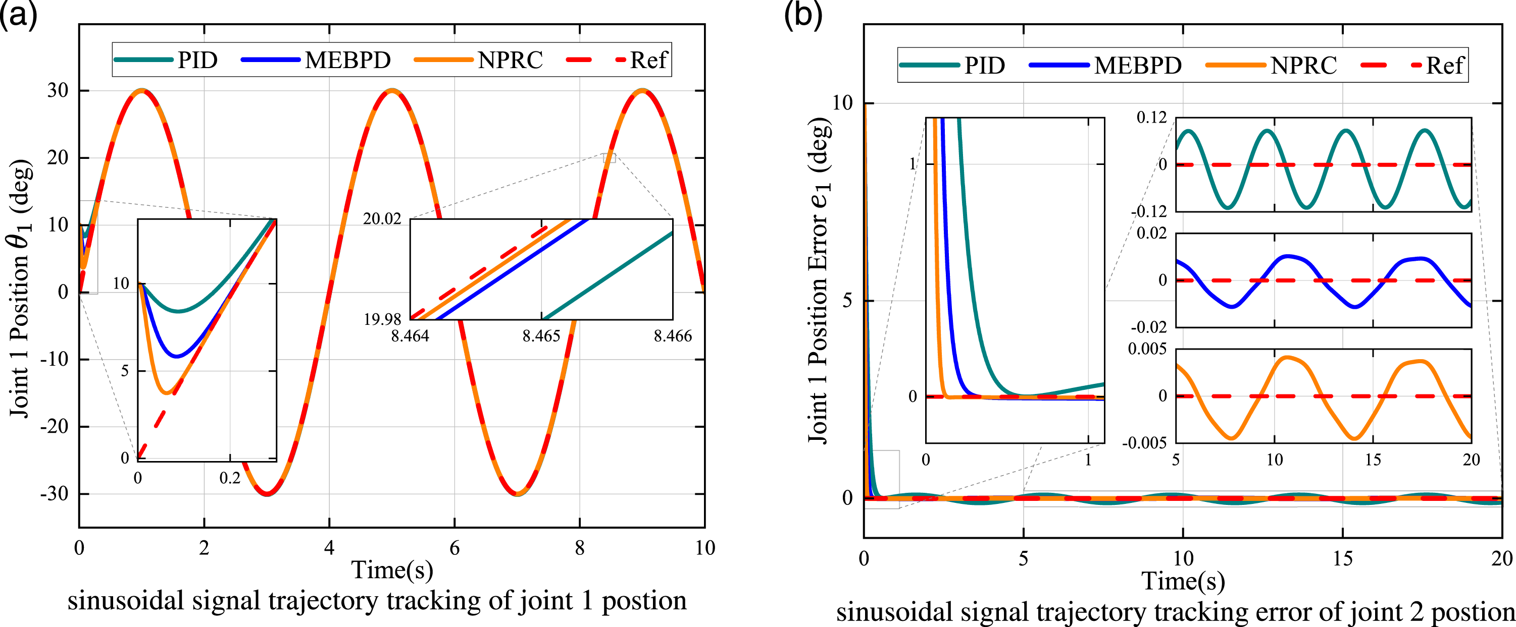

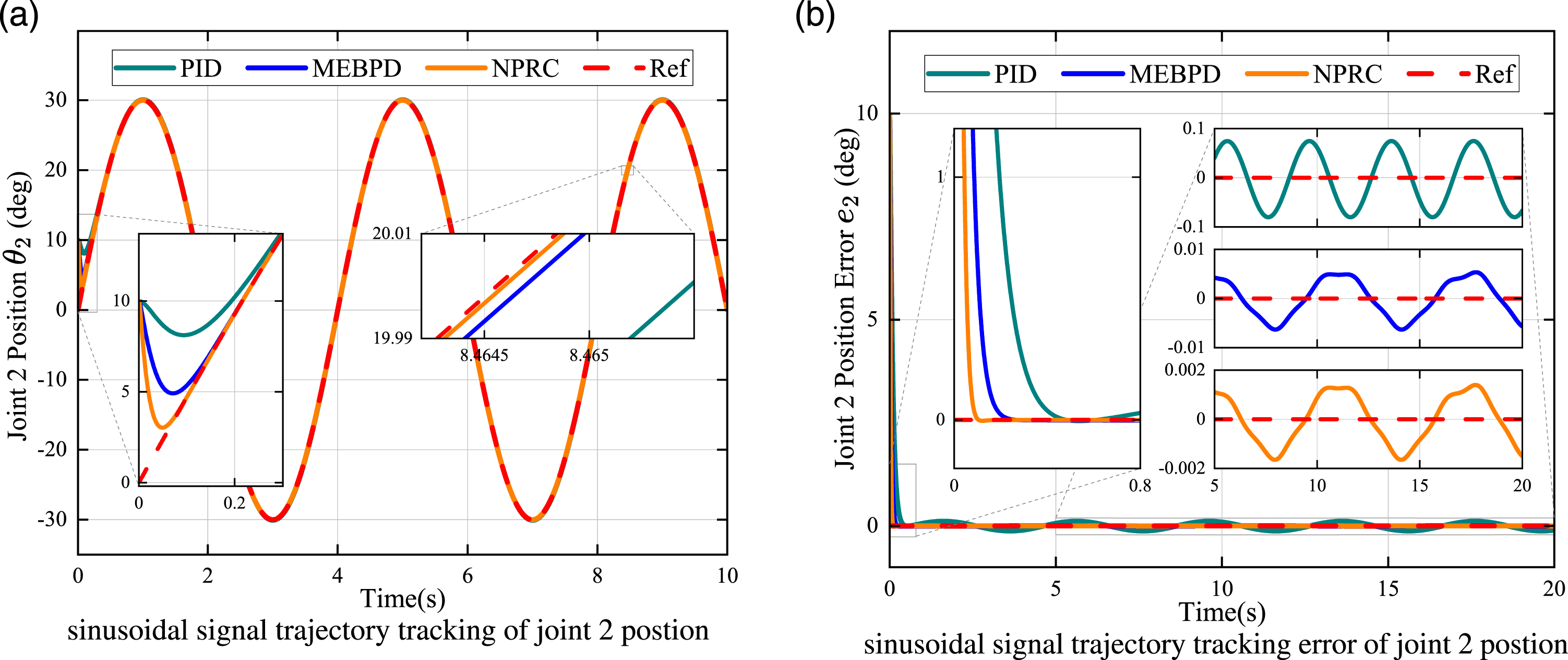
From the above simulation results, it can be concluded that the proposed controller can theoretically ensure the superior dynamic performance of the 2-DOF planar robotic arm.

4.3. Experimental platform introduction

The main experimental setup mainly consists of a 2-DOF planar robotic arm, personal computer, CSPACE-RT control system, and loads of different masses as shown in Figure 6. Each joint of the 2-DOF planar robotic arm integrates a 20,000-line incremental encoder, a 17-bit absolute value encoder, a frameless torque motor, a harmonic reducer, and a servo drive. The incremental encoder is used to detect the rotation angle of the motor, and the absolute value encoder is used to detect the angle of the output shaft (link) of the harmonic reducer. The CSPACE-RT control platform enables efficient verification of control algorithms and is a rapid controller prototype (real-time) system composed of digital signal processors (DSP).

Figure 6.

Experimental setup of 2-DOF planar robotic arm.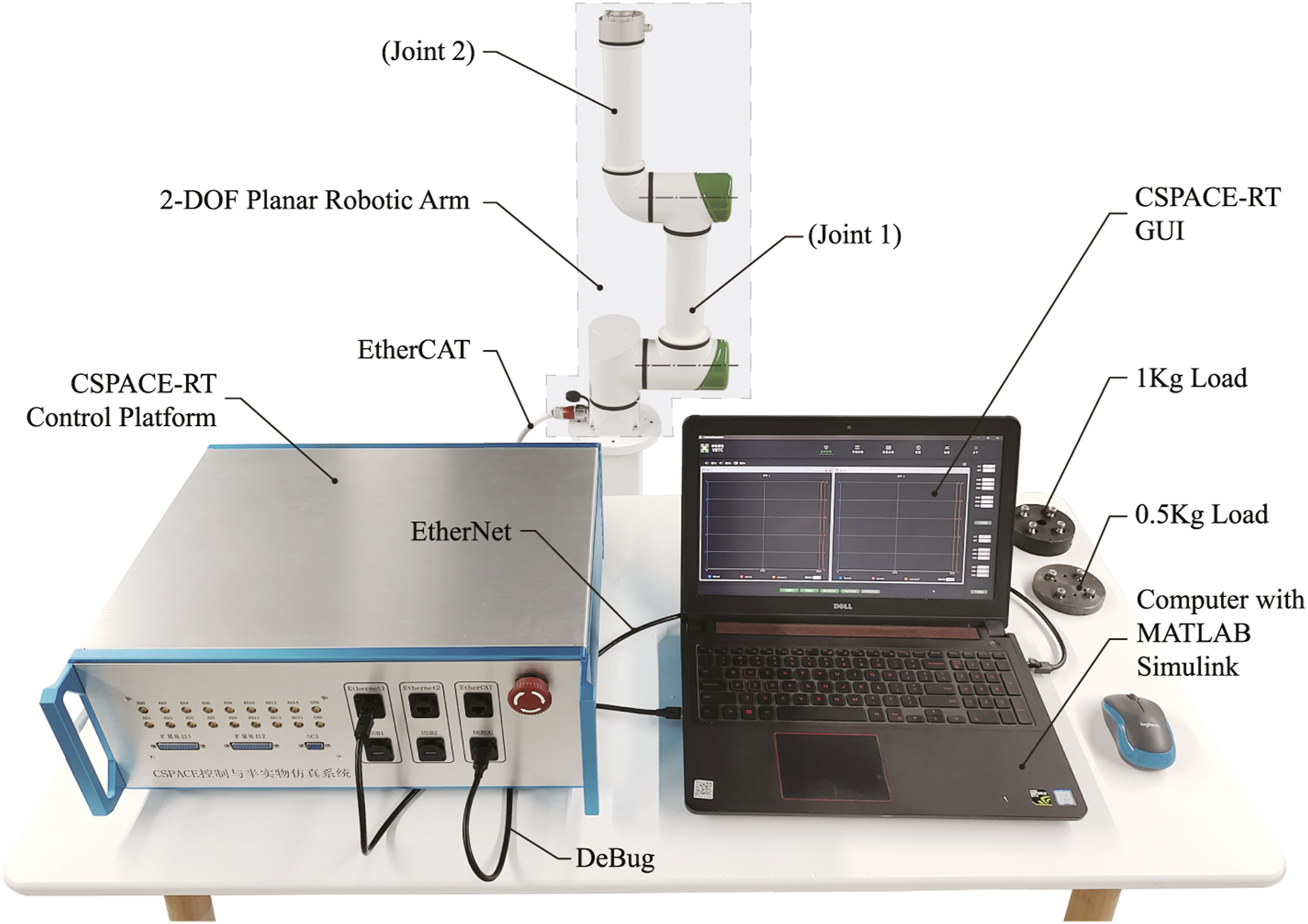

The software for the CSPACE-RT control system uses the Texas Instruments C2000 Processor Embedded Encoder Support Package based on MATLAB R2020b or later. The support package integrates all peripheral I/O drivers of DSP C2000 in a graphical way, which is convenient for users to integrate the control algorithm into the experimental object and realize the fast verification of the algorithm. By associating MATLAB/Simulink with CCS compiling environment in advance, the Simulink model can be converted into a real-time executable file through an embedded coder toolbox and downloaded to the DSP chip for running. The CSPACE-RT GUI is a graphical user interface developed based on the MATLAB App Designer environment. On the right side of the GUI, we can modify six data under different group numbers to change different variables. Up to 42 variables can be modified to realize online modification of variable values. There are three windows in the middle of the interface, and each window can display the curve of three variables, equivalent to a real-time display of nine variable data. The simple interface operation function provides great convenience for our experiment.

The CSPACE-RT control system is jointly developed with MATLAB/Simulink, enabling the simulation to be quickly transferred to real-time control and speeding up the algorithm development cycle. This development method is convenient for researchers to verify the algorithm design and performance. The flowchart for developing and verifying the control algorithms using the CSPACE-RT control system is shown in Figure 7.

Figure 7.

Flowchart of the algorithm development using the CSPACE-RT control system.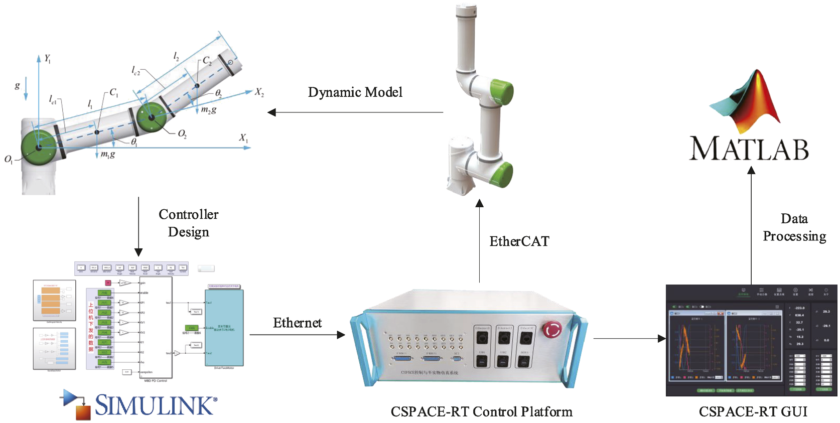

The steps for developing and validating an algorithm implementation using the CSPACE-RT control system are as follows.

Step 1

Dynamic model and controller design in MATLAB/Simulink based on the controlled object.

Step 2

The conversion of the model into C codes using MATLAB, which can be downloaded and run on the CSPACE-RT control platform.

Step 3

Compile and download the generated C codes to the CSPACE-RT control platform using the Code Composer Studio (CCS) software.

Step 4

Set the sampling time to 0.005 s and run the C codes on the CSPACE-RT control platform. Real-time adjustment of critical parameters of the algorithm by observing the controlled object motion curves in the GUI and saving and processing motion data.

4.4. Experiment validation

Based on the 2-DOF planar robotic arm platform, the performance of each control algorithm in practical applications is further investigated, and the results are analyzed and compared. Similarly, the relevant control parameters are selected with reference to Table 3, where the performance metrics include transient performance, steady-state performance, and robust performance for varying load perturbations. The control experiment is summarized in three steps: (i) The driver receives the joint position of the robotic arm from the absolute encoder. (ii) The angle and current signals from the drive are transmitted to the CSPACE-RT controller via the Control Automation Technology Ethernet (EtherCAT) bus, which calculates the control signals in combination with the control algorithm. (iii) The control signals are transmitted to the drive via the EtherCAT bus and amplified to drive the motor movement.

4.4.1. Transient performance

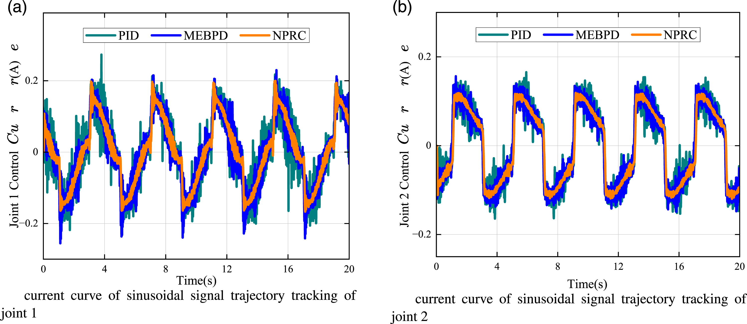
The step signal amplitudes used in the experiment are both 10°. Figure 8(a) and (b) show experimental curves of the step response of the 2-DOF planar robotic arm. For both joint 1 and joint 2, the NPRC control algorithm reached the desired position faster than the other control algorithms. More details can be obtained from Table 4, where T_r represents the rise time, T_s represents the steady-state time, and IM represents the degree of improvement relative to other control algorithms. For all control algorithms, the steady-state error of joint 1 is larger than that of joint 2, and joint 1 produces more chatter than joint 2, which may be due to the influence of joint 1 by the weight of joint 2. Also, the NPRC control algorithm achieves steady-state with less error and chatter than other control algorithms, which is attributable to the robustness term of the controller.

Figure 8.

The position step response experimental curves of the two joints of the 2-DOF planar robotic arm.

Table 4.

Comparison of sinusoid signal tracking simulation data under different control algorithms.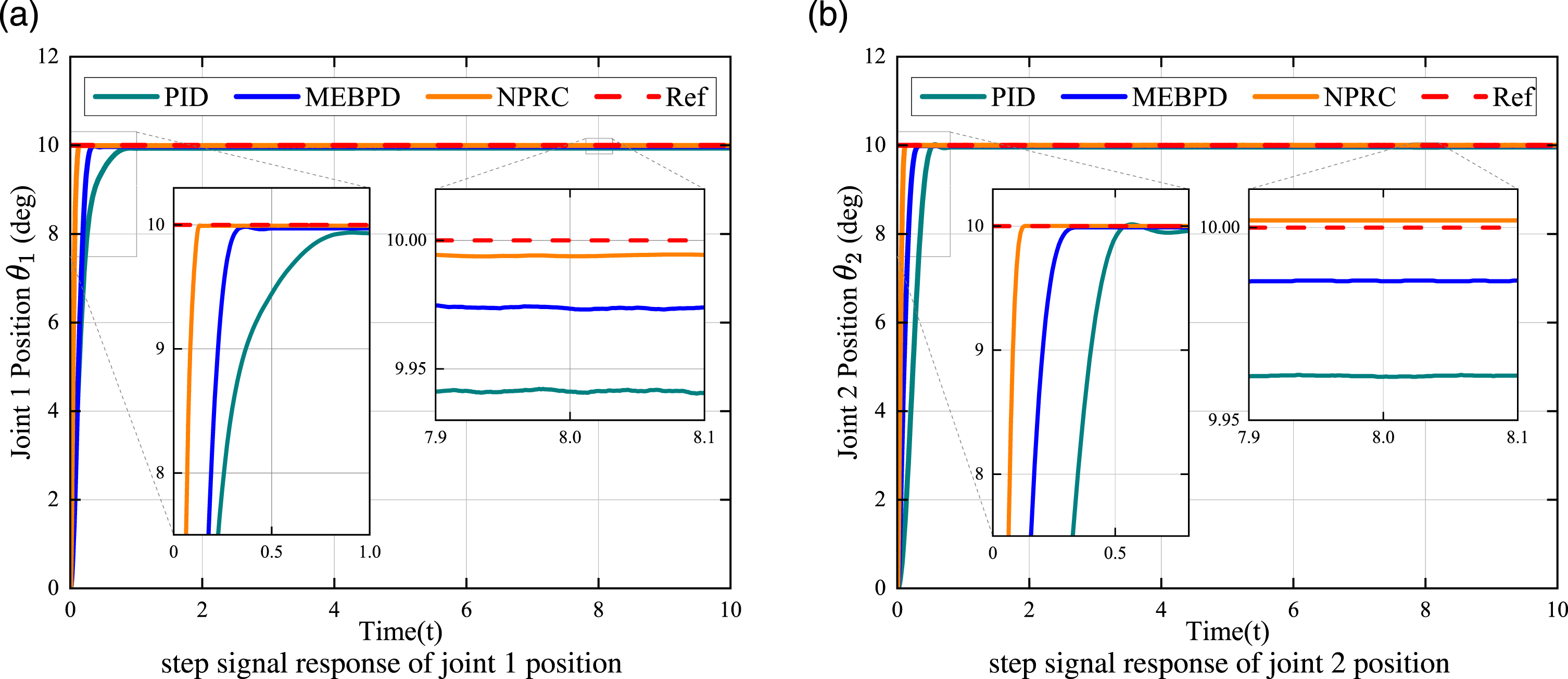

Control algorithm	Joint 1		Joint 2
Control algorithm	T_r1(s)	T_s1(s)	T_r2(s)	T_s2(s)
PID	0.897	1.027	0.541	0.804
MEBPD	0.364	0.497	0.324	0.345
NPRC	0.134	0.148	0.132	0.148
IM(PID)	85.06%	85.59%	75.60%	81.59%
IM(MEBPD)	63.19%	70.22%	59.26%	57.10%

Specifically, the steady-state errors of the PID, MEBPD, and NPRC control algorithms are e₁ = 0.0578 ∼ 0.0661 deg, e₂ = 0.0356 ∼ 0.0382 deg, e₁ = 0.0243 ∼ 0.0277 deg, e₂ = 0.0088 ∼ 0.0111 deg, and e₁ = 0.0029 ∼ 0.0068 deg, e₂ = −0.0018 ∼ − 0.0011 deg, respectively.

4.4.2. Steady-state performance

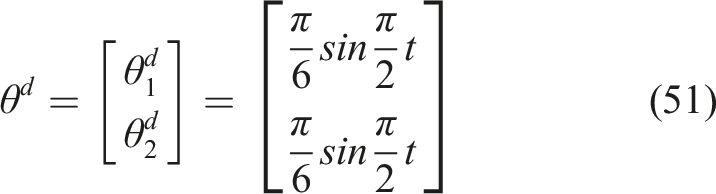
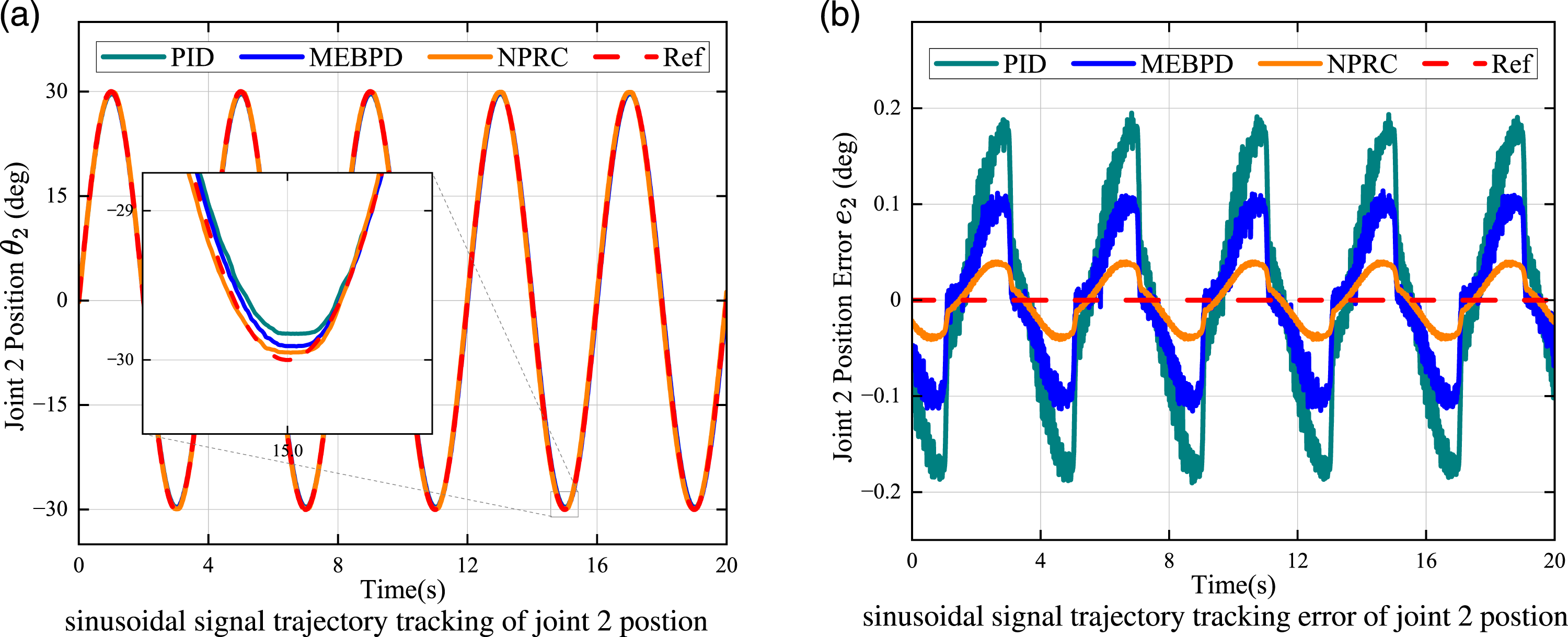
Figures 9(a) and 10(a) indicate joint position curves in the sinusoidal signal tracking experimental. Likewise, the tracked sinusoidal signal can be obtained from equation (51). The tracking performance comparison of different control algorithms can be obtained from the tracking error curves in Figures 9(b) and 10(b). Specifically, the tracking errors of the PID, MEBPD, and NPRC control algorithms are e₁ = 0.0578 ∼ 0.0661 deg, e₂ = 0.0356 ∼ 0.0382 deg, e₁ = 0.0243 ∼ 0.0277 deg, e₂ = 0.0088 ∼ 0.0111 deg, and e₁ = 0.0029 ∼ 0.0068 deg, e₂ = −0.0018 ∼ − 0.0011 deg, respectively. The NPRC control algorithm offers better trajectory tracking performance owing to its smaller tracking error. Figure 11(a) and (b) show the control current curves for joint 1 and joint 2 tracking sinusoidal signals, where the NPRC control algorithm had smaller control current fluctuations than the other control algorithms, especially for Current₂.

Figure 9.

The sinusoidal signal trajectory tracking experimental curves of the joint 1 of the 2-DOF planar robotic arm.

Figure 10.

The sinusoidal signal trajectory tracking experimental curves of the joint 2 of the 2-DOF planar robotic arm.

Figure 11.

The sinusoidal signal trajectory tracking experimental control current curves of the two joints of the 2-DOF planar robotic arm.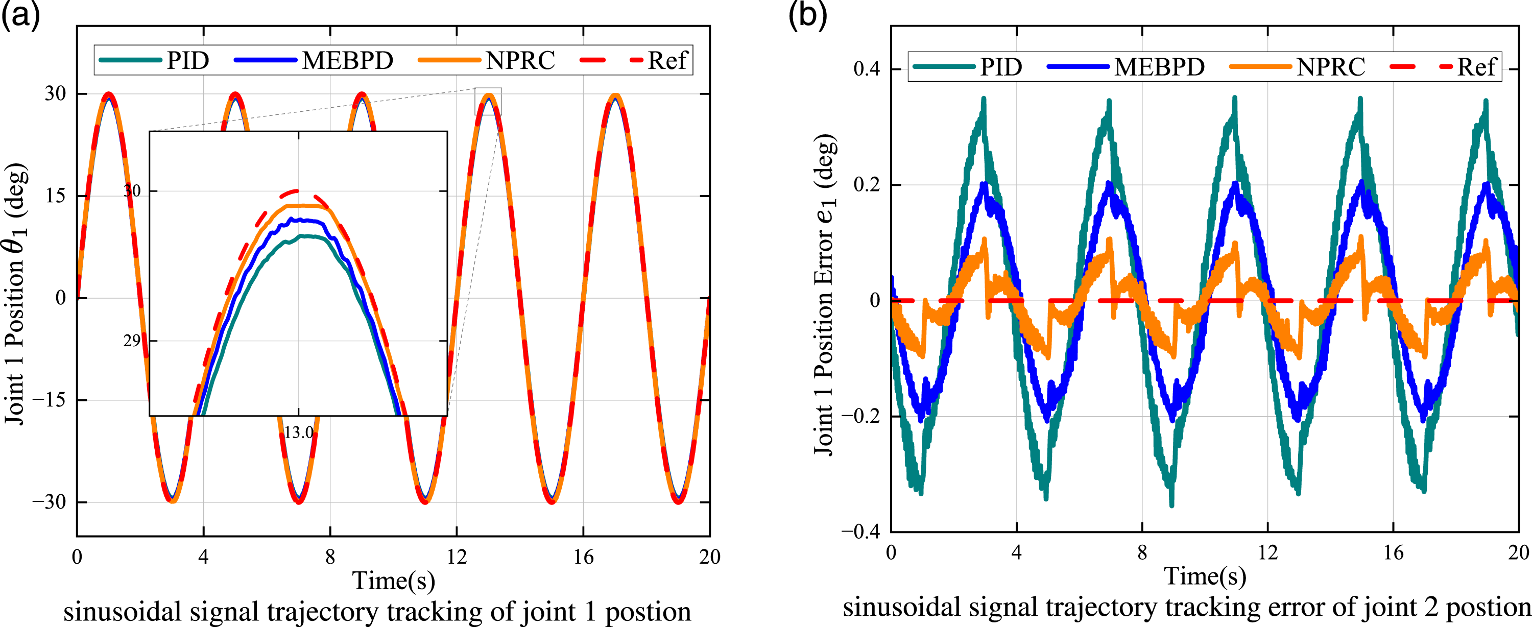

4.4.3. Robustness against the load variation

Changing loads can affect the uncertainty (both structural and parametric) within the robotic arm system indirectly. By installing loads of different masses (0 kg, 0.5 kg, and 1.0 kg) on the end flange of the 2-DOF planar robotic arm and making it follow the desired sinusoidal signals, the robustness of different algorithms to load disturbances is verified. Experimental details of the results can be obtained from the error curves from Figure 12(a)–(f). The vertical comparison shows a reasonable increase in tracking error with increasing load for both joints, with a more significant increase in tracking error for joint 2.

Figure 12.

The sinusoidal signal trajectory tracking experimental curves of the two joints of the 2-DOF planar robotic arm with different loads.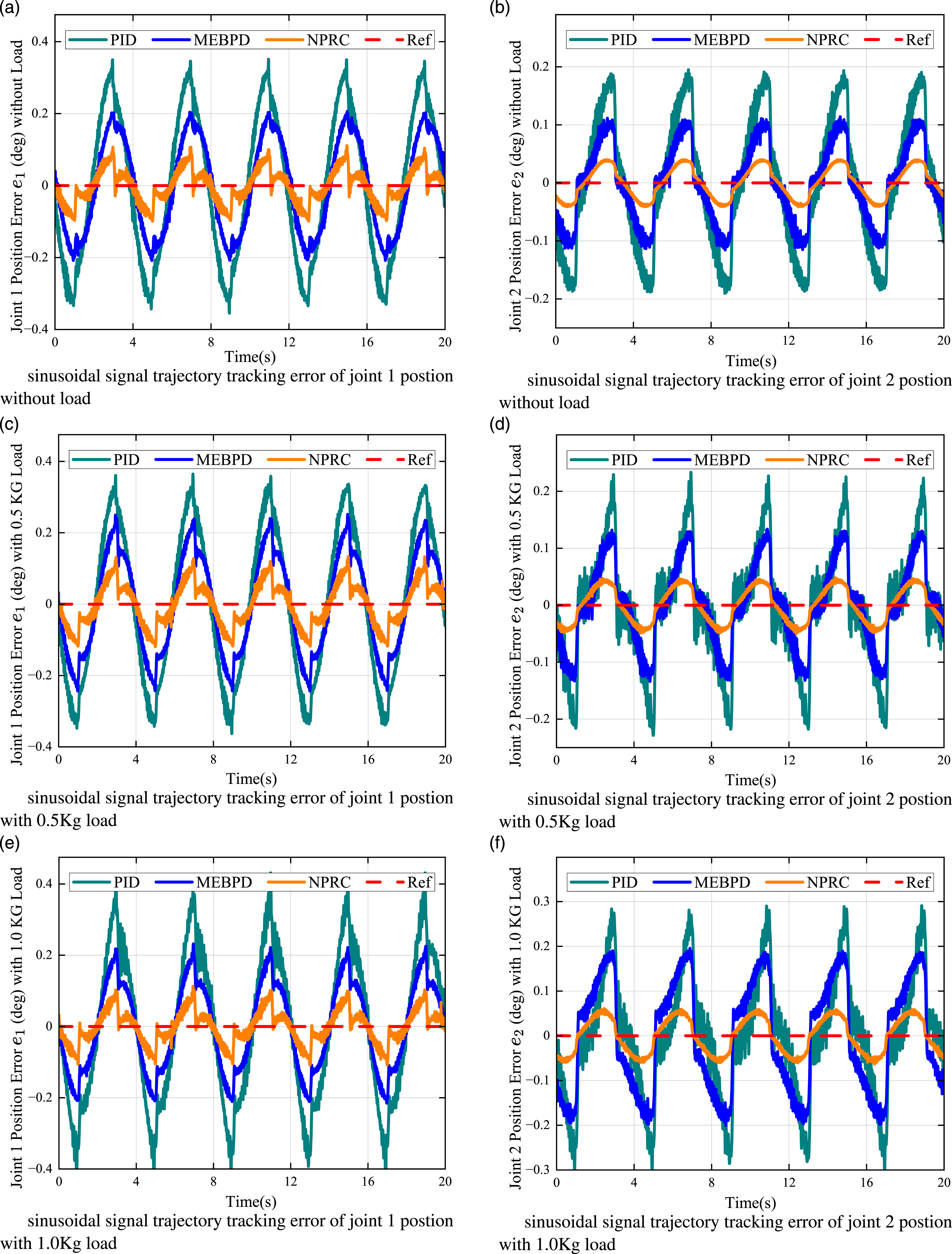

The results of the above experiments are analyzed quantitatively in Table 5 to make the side-by-side comparisons more concrete. MAXE and RMSE are the root mean square values of the maximum joint position error and the joint position error, respectively. They are defined by equation (56) and equation (57). While IM is the improved value with respect to the PID and MEBPD control schemes

M A X E = \max (| e_{i} |)

(56)

R M S E = \sqrt{\frac{1}{N} \sum_{i = 1}^{N} e_{i}^{2}}

(57)

where e_i is the tracking error of the ith sampling point and N is the total number of sampling points. Table 5 illustrates that the NPRC control algorithm has smaller RMSE and MAXE compared to the PID and MEBPD control algorithms with significant improvement in each case.

Table 5.

Tracking performance comparison of 2-DOF planar robotic arms under different loads.

Load	Control algorithm	Joint 1		Joint 2
Load	Control algorithm	MASE	RMSE	MASE	RMSE
0 kg load	PID	0.3513	0.2031	0.1950	0.1119
	MEBPD	0.2061	0.1318	0.1140	0.0659
	NPRC	0.1110	0.0464	0.0400	0.0266
	IM(PID)	68.41%	77.16%	79.51%	76.26%
	IM(MEBPD)	46.16%	64.79%	64.95%	59.67%
0.5 kg load	PID	0.3645	0.2085	0.2333	0.1020
	MEBPD	0.2515	0.1393	0.1335	0.0722
	NPRC	0.1329	0.0599	0.0482	0.0302
	IM(PID)	63.54%	71.28%	79.34%	70.37%
	IM(MEBPD)	47.15%	57.00%	63.91%	58.12%
1.0 kg load	PID	0.4312	0.2097	0.2910	0.1318
	MEBPD	0.2318	0.1228	0.1955	0.1246
	NPRC	0.1126	0.0462	0.0608	0.0392
	IM(PID)	73.89%	77.95%	79.12%	70.25%
	IM(MEBPD)	51.44%	62.37%	68.92%	68.51%

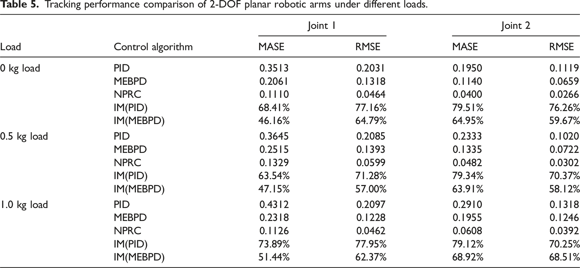
Overall, the NPRC control algorithm provides faster response speed for the 2-DOF planar robotic arm system compared to the experimental PID control algorithm and MEBPD control algorithm, while ensuring better steady-state performance due to the robustness term of the proposed method. The smaller fluctuation in tracking error of the NPRC control algorithm during load variation indicates that the proposed controller has better tracking performance and robustness against uncertainties.

5. Conclusions

This paper proposes a new practical robust control scheme for the robotic arm, and the controller is verified with excellent dynamic performance and robustness through numerical simulations and experiments. The energy-based Lagrangian method is used to model the dynamics of the system, and both Coulomb friction and viscous friction are considered to suppress the reversal chattering. The uncertainties within the system are assumed to be time-varying but bounded, which is represented uniformly by a function. The proposed controller consists of a model- and error-based PD term and an error-based robust term containing the upper bound of the uncertainty term. Further, the Lyapunov minimax approach theoretically proves the proposed controller to guarantee the controlled system with UB and UUB. Based on the 2-DOF planar robotic arm experimental platform, the self-developed rapid controller prototype CSPACE-RT is used to improve the rate of dynamic load and multi-algorithm debugging processes. The proposed controller provided excellent transient, steady-state performance, trajectory tracking capability, and robustness through numerical simulations and experimental results compared with MEBPD and PID control algorithms. We will implement this control algorithm in engineering practice to solve other control problems of time-varying nonlinear systems in the future.

Footnotes

Declaration of conflicting interests

The author(s) declared no potential conflicts of interest with respect to the research, authorship, and/or publication of this article.

Funding

The author(s) disclosed receipt of the following financial support for the research, authorship, and/or publication of this article: This work was supported by National Natural Science Foundation of China [Grant No.52305084]; the Key Research and Development Program of AnHui Province [Grant No.2022a05020014]; the Fundamental Research Funds for the Central Universities [Grant No. PA2021KCPY0035]; the University Synergy Innovation Program of Anhui Province [Grant No. GXXT-2021-010]; the Key Laboratory of Construction Hydraulic Robots of Anhui Higher Education Institutes, Tongling University [Grant No. TLXYCHR-O-21ZD01]; and the Pioneer Program Project of Zhejiang Province [Grant No.2022C03018].

ORCID iDs

Shengchao Zhen

Chaoqun Meng

Xiaoli Liu

References

Aboserre

El-Badawy

(2021) Robust integral sliding mode control of tower cranes. Journal of Vibration and Control 27(9–10): 1171–1183.

Alandoli

Lee

Vijayakumar

, et al. (2022) Dynamic model and integrated optimal controller of hybrid arms robot for laser contour machining. Journal of Vibration and Control 29(13): 10775463221090000.

Ang

Chong

(2005) PID control system analysis, design, and technology. IEEE Transactions on Control Systems Technology 13(4): 559–576. DOI: 10.1109/TCST.2005.847331.

Baek

Jin

Han

(2016) A new adaptive sliding-mode control scheme for application to robot manipulators. IEEE Transactions on Industrial Electronics 63(6): 3628–3637. DOI: 10.1109/TIE.2016.2522386.

Chen

(1986) On the deterministic performance of uncertain dynamical systems. International Journal of Control 43(5): 1557–1579. DOI: 10.1080/00207178608933559.

Chen

(2021) On active disturbance rejection control for a class of uncertain systems with measurement uncertainty. IEEE Transactions on Industrial Electronics 68(2): 1475–1485. DOI: 10.1109/TIE.2020.2970623.

Corless

Leitmann

(1981) Continuous state feedback guaranteeing uniform ultimate boundedness for uncertain dynamic systems. IEEE Transactions on Automatic Control 26(5): 1139–1144. DOI: 10.1109/TAC.1981.1102785.

Dean-Leon

Ramirez-Amaro

Bergner

, et al. (2017) Integration of robotic technologies for rapidly deployable robots. IEEE Transactions on Industrial Informatics 14(4): 1691–1700.

Fareh

Khadraoui

Abdallah

, et al. (2021) Active disturbance rejection control for robotic systems: a review. Mechatronics 80: 102671. DOI: 10.1016/j.mechatronics.2021.102671.

10.

Figueredo

LFC

Adorno

Ishihara

(2021) Robust H∞ kinematic control of manipulator robots using dual quaternion algebra. Automatica 132: 109817. DOI: 10.1016/j.automatica.2021.109817.

11.

Gaidhane

Nigam

Kumar

, et al. (2019) Design of interval type-2 fuzzy precompensated PID controller applied to two-DOF robotic manipulator with variable payload. ISA Transactions 89: 169–185. DOI: 10.1016/j.isatra.2018.12.030.

12.

Han

(2009) From PID to active disturbance rejection control. IEEE Transactions on Industrial Electronics 56(3): 900–906. DOI: 10.1109/TIE.2008.2011621.

13.

Islam

Liu

(2011) Robust sliding mode control for robot manipulators. IEEE Transactions on Industrial Electronics 58(6): 2444–2453. DOI: 10.1109/TIE.2010.2062472.

14.

Lai

Zhang

Wang

, et al. (2017) Position-posture control of a planar four-link underactuated manipulator based on genetic algorithm. IEEE Transactions on Industrial Electronics 64(6): 4781–4791. DOI: 10.1109/TIE.2017.2668979.

15.

Lee

Kim

Al Amin

MAU

(2022) Control framework for collaborative robot using imitation learning-based teleoperation from human digital twin to robot digital twin. Mechatronics 85: 102833.

16.

Liu

Chen

Zhao

, et al. (2016) Smooth trajectory planning for a parallel manipulator with joint friction and jerk constraints. International Journal of Control, Automation and Systems 14(4): 1022–1036. DOI: 10.1007/s12555-014-0495-4.

17.

Huang

(2020) Adaptive neural-network controller for an uncertain rigid manipulator with input saturation and full-order state constraint. IEEE Transactions on Cybernetics 52(5): 1–9. DOI: 10.1109/TCYB.2020.3022084.

18.

Nikdel

Badamchizadeh

Azimirad

, et al. (2017) Adaptive backstepping control for an n-degree of freedom robotic manipulator based on combined state augmentation. Robotics and Computer-Integrated Manufacturing 44: 129–143. DOI: 10.1016/j.rcim.2016.08.007.

19.

Noble

Daniel

(1977) Applied Linear Algebra. Englewood Cliffs, NJ: Prentice-Hall, Vol. 477.

20.

Rad

Tamizi

Azmoun

, et al. (2020) Experimental study on robust adaptive control with insufficient excitation of a 3-DOF spherical parallel robot for stabilization purposes. Mechanism and Machine Theory 153: 104026. DOI: 10.1016/j.mechmachtheory.2020.104026.

21.

Santos

KRS

Villani

de Oliveira

, et al. (2022) Comparison of visual servoing technologies for robotized aerospace structural assembly and inspection. Robotics and Computer-Integrated Manufacturing 73: 102237. DOI: 10.1016/j.rcim.2021.102237.

22.

Shi

Zhang

, et al. (2021) Human-centred adaptive control of lower limb rehabilitation robot based on human–robot interaction dynamic model. Mechanism and Machine Theory 162: 104340. DOI: 10.1016/j.mechmachtheory.2021.104340.

23.

Sivčev

Coleman

Omerdić

, et al. (2018) Underwater manipulators: a review. Ocean Engineering 163: 431–450. DOI: 10.1016/j.oceaneng.2018.06.018.

24.

Solanes

Gracia

Muñoz-Benavent

, et al. (2018) Adaptive robust control and admittance control for contact-driven robotic surface conditioning. Robotics and Computer-Integrated Manufacturing 54: 115–132. DOI: 10.1016/j.rcim.2018.05.003.

25.

Sumartojo

Lugli

(2022) Lively robots: robotic technologies in covid-19. Social & Cultural Geography 23(9): 1220–1237.

26.

Tang

Chen

Wang

, et al. (2020) Recognition and localization methods for vision-based fruit picking robots: a review. Frontiers in Plant Science 11: 510. DOI: 10.3389/fpls.2020.00510.

27.

Troccaz

Dagnino

Yang

(2019) Frontiers of medical robotics: from concept to systems to clinical translation. Annual Review of Biomedical Engineering 21(1): 193–218. DOI: 10.1146/annurev-bioeng-060418-052502.

28.

Villani

De Wit

Brogliato

(1999) An exponentially stable adaptive control for force and position tracking of robot manipulators. IEEE Transactions on Automatic Control 44(4): 798–802. DOI: 10.1109/9.754821.

29.

Chen

(2002) Robust H/spl infin/control for uncertain stochastic systems with state delay. IEEE Transactions on Automatic Control 47(12): 2089–2094. DOI: 10.1109/TAC.2002.805670.

30.

Yang

(2018) Dynamic modelling and adaptive robust tracking control of a space robot with two-link flexible manipulators under unknown disturbances. International Journal of Control 91(4): 969–988. DOI: 10.1080/00207179.2017.1300837.

31.

Yin

Pan

(2018) Direct adaptive robust tracking control for 6 DOF industrial robot with enhanced accuracy. ISA Transactions 72: 178–184. DOI: 10.1016/j.isatra.2017.10.007.

32.

Yin

Pan

Cai

(2021) Robust adaptive fuzzy sliding mode trajectory tracking control for serial robotic manipulators. Robotics and Computer-Integrated Manufacturing 72: 101884. DOI: 10.1016/j.rcim.2019.101884.

33.

Zamani

Etedali

(2023) Optimal fractional-order pid control design for time-delayed multi-input multi-output seismic-excited structural system. Journal of Vibration and Control 29(3–4): 802–819.

34.

Zhai

(2021) A novel non-singular terminal sliding mode trajectory tracking control for robotic manipulators. IEEE Transactions on Circuits and Systems II: Express Briefs 68(1): 391–395. DOI: 10.1109/TCSII.2020.2999937.