
Abstract
Multi-scale ensemble learning combines different scales of feature resolution, thereby improving fault diagnostic accuracy. However, the effectiveness of different information scales in characterizing fault features under time-varying speed conditions varies with speed. It is difficult for existing ensemble strategies to ensure the effectiveness of feature information when ensemble multi-scale feature information is involved. Accordingly, we propose an uncertainty-driven dynamic ensemble Bayesian convolutional neural network (DEBCNN) framework. The uncertainty of the results of different scale models was used to dynamically determine their weights in the ensemble framework, which reduced the influence of irrelevant features on the diagnostic results. By employing the proposed dynamic ensemble strategy, the ensemble framework can utilize fault feature information corresponding to different rotational speeds in the final diagnostic results. Experiments on motor and bearing datasets illustrate the superiority of this strategy over other techniques. This study provides useful insights for further research in the field of fault diagnosis of rotating machinery at time-varying speeds.
Keywords
1. Introduction
Rotating machinery, such as motors and bearings, has been utilized extensively in the industrial sector and is a crucial component of manufacturing machinery for the aerospace, wind energy, transportation, and rail industries (Liu et al., 2023; Zhu et al., 2023). However, in the real world, owing to complex working conditions, continuous operation, and other factors, rotating machinery is prone to malfunction. If not diagnosed and repaired immediately, these malfunctions may seriously impact the system (Osornio-Rios et al., 2023; Xu et al., 2024).
Working state recognition, which analyzes the signal characteristics of rotating machines during operation, has been widely used in electric motors, bearings, gearboxes, and other rotating machines. Gangsar and Tiwari summarized in detail the application of signal analysis in motor fault diagnosis (Gangsar and Tiwari, 2020). Ruan et al. accurately diagnosed various types of bearing faults by combining signal processing and artificial intelligence algorithms (Ruan et al., 2023). Zhou and Tang used vibration signal processing and wavelet neural networks to predict the remaining useful life (Zhou and Tang, 2023). Feng reviewed signal processing-based gear wear monitoring, prediction, and health management technologies in detail and showed that vibration-based gear wear monitoring and remaining life prediction technologies have good application prospects (Feng et al., 2023a). Feng used cyclic correntropy and Wasserstein distance to construct gearbox health indicators, combined with a gated recurrent unit (GRU) network to achieve vibration-based prediction of gear health (Feng et al., 2023b).
Under time-varying speed conditions, the signals of rotating machines are no longer periodic, and the spectral features related to the current state of the machine become ambiguous, which further increases the difficulty of fault diagnosis in rotating machines. Therefore, fault diagnosis under time-varying speed conditions has become a popular research topic. Traditionally, order tracking (Fyfe and Munck, 1997) and time–frequency analysis can improve diagnostic accuracy under time-varying speed conditions. Wang et al. proposed computed order tracking (COT) and variational modal decomposition based on the fault diagnosis of rolling bearings under variable speed conditions (Wang et al., 2017). Yu et al. proposed a multi-synchrosqueezing transform (MSST) for machine fault diagnosis under highly time-varying speeds (Yu et al., 2019). However, order tracking requires the extraction of current rotational speed information, time–frequency analysis has a parameter selection process in the middle, and both order tracking and time–frequency analysis require significant computational effort, which makes it difficult to meet the requirements in the context of big data.
Deep learning methods, such as convolutional neural networks (CNNs) (Gong et al., 2024; Tarek and Sameh, 2024), deep belief networks (DBNs) (Pan et al., 2023), and auto-encoders (AE) (Zhao et al., 2023), have been successfully applied to industrial fault diagnosis. However, achieving good diagnostic performance with deep learning methods typically requires large amounts of independent and identically distributed data, which are difficult to obtain in real-world scenarios, especially under variable-speed conditions. During the fault feature learning phase, the nonstationarity of fault features under varying speeds complicates the learning of the fault models. Furthermore, in the diagnosis phase, discrepancies between the learned model features and features to be diagnosed can lead to overfitting. Therefore, improving the ability of models to learn fault features from non-identically distributed data will further improve the diagnostic accuracy of deep-learning-based fault diagnosis methods under time-varying speed conditions.
Ensemble learning integrates multiple learners to create a combined model with higher accuracy than any single model. Wang et al. used ensemble learning to diagnose unbalanced fault data conditions and improved the ability of the model to handle unbalanced data (Wang et al., 2023a). Ye et al. used ensemble learning to integrate multi-sensor data for bearings, which improved the ability of the model to learn fault features under noisy conditions and improved the ability of the model to diagnose faults in such environments (Ye et al., 2024). Li et al. used ensemble learning to enable the model to learn latent fault features from data across different domains, thereby improving the accuracy of cross-domain fault diagnosis (Li et al., 2021). As a result, ensemble learning effectively addresses the degradation of fault diagnostic accuracy caused by overfitting individual models when dealing with non-independent and identically distributed data.
The ensemble strategy is crucial to the success of ensemble learning because it directly determines the contribution of different submodels to the final diagnostic results. Commonly used voting methods in ensemble learning include majority voting (Imane et al., 2023), weighted voting (Wang et al., 2023c), and Dempster–Shafer (DS) evidence theory (Wang et al., 2023b). Zhou et al. (2023) employed a weighted-average strategy to combine two ResNet18 models with two shallow CNN models for fault diagnosis in rotating machinery (Zhou et al., 2023). Xu et al. combined transmission vibration signals from both the time and frequency domains using weighted voting to enhance the robustness and generalization of transmission fault diagnosis (Xu et al., 2022). Wang et al. applied the DS evidence theory in fault diagnosis using multiple sensors and selected key information from multiple sensor features to diagnose the final fault type (Wang et al., 2023b).
However, most of the ensemble strategies mentioned above rely on the accuracy of the submodels to determine their weights in the ensemble model. The main reasons for the degradation of diagnostic performance under time-varying speed conditions is the fact that the model learns fault features from ambiguous data and the learned features deviate from those of the samples to be diagnosed. These two issues lead to uncertainty in the fault diagnosis results under time-varying conditions, which, in turn, reduces the diagnostic accuracy. To address this issue, this study proposes a multi-scale dynamic ensemble strategy based on model uncertainty for the effective diagnosis of rotating machinery faults at time-varying speeds. The main contributions of this study are as follows: (1) We provide a new perspective by transforming the fault diagnosis problem under variable-speed conditions into an uncertainty-reduction problem. The proposed model could be applied to a range of time-varying speed intervals. (2) The uncertainty in the diagnostic results for different time-varying speed samples was measured using Bayesian principles and Monte Carlo sampling. (3) We propose an uncertainty-based dynamic ensemble strategy for the fault diagnosis of rotating machinery under time-varying speed conditions, which addresses the uncertainty of the submodels and improves fault diagnosis performance through more fundamental uncertainty reduction.
2. Methodology
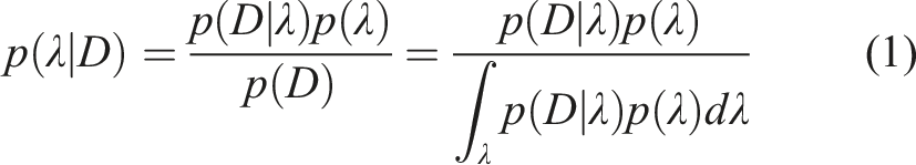
2.1. Bayesian CNNs
The optimum parameters in the standard CNN model are the point estimates of the corresponding parameters, which represent fixed values. These values are obtained through forward propagation of the training samples and backward error updating. Because the parameters are fixed, the uncertainty of the decision cannot be reflected after multiple inputs into the trained model, leading to several diagnoses of the same value and, ultimately, the same decision. While the training optimization objective of the Bayesian CNN (BCNN) model shifts from finding the best parameters to finding the best parameter distribution interval, also known as the posterior distribution
The likelihood function
2.2. Variational inference
Variational distribution
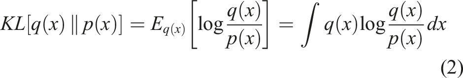
Therefore, the KL between the variational distribution
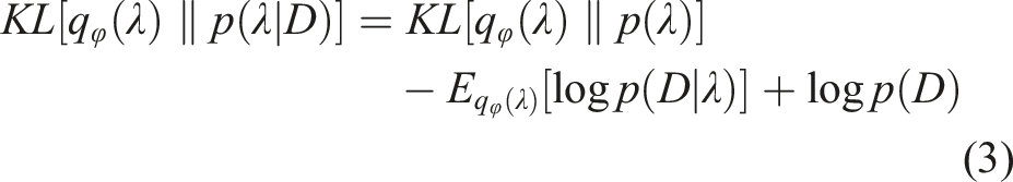
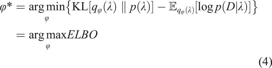
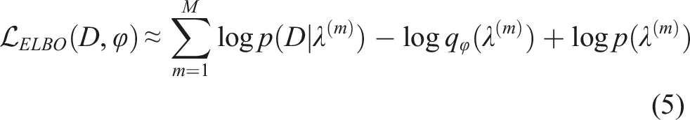
Assuming that the parameters are independent of each other, the loss function of the network can be obtained using the Monte Carlo sampling approximation, as follows:
2.3. Dynamic ensemble strategy
The BCNN parameter distribution
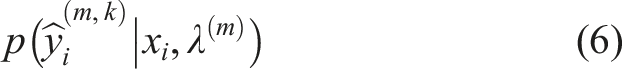
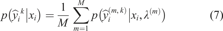
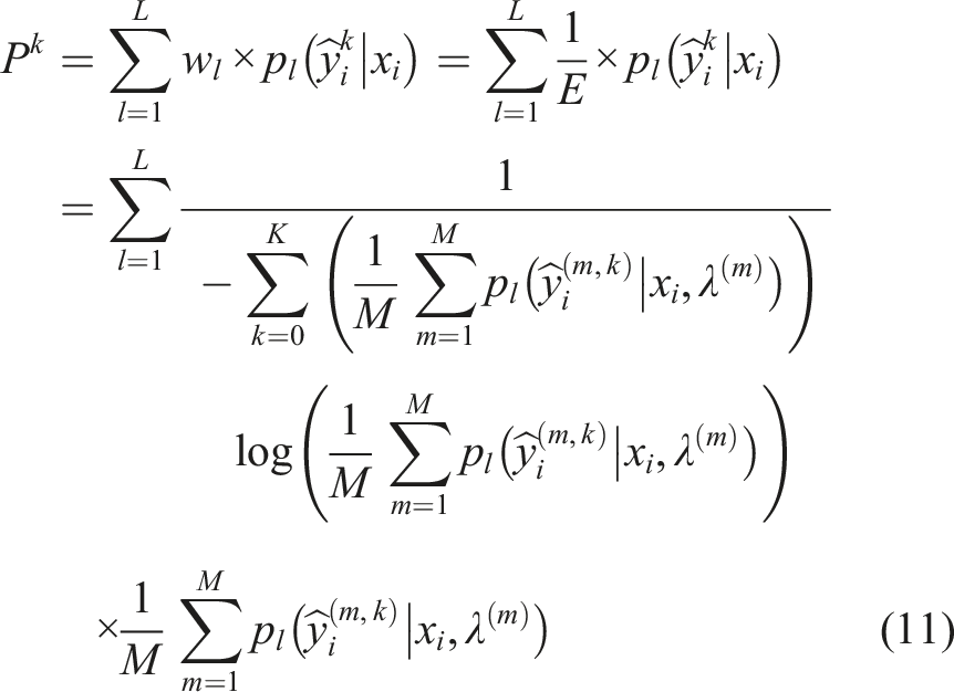
The sampling results avoid the influence of individual experiments on the diagnostic results and render the predicted probabilities of different fault types more reliable. The uncertainty in the diagnostic results is reflected in the difference between the predicted probabilities of the correct and incorrect fault labels. When it is difficult for the model to classify the samples, there is a proximity of the predicted probabilities between different fault types, which leads to a higher overall entropy value of the predicted probabilities. However, when the model has an outstanding predicted probability of a certain fault type, the predicted probabilities of the other fault types are extremely small, which leads to a lower overall entropy value of the predicted probabilities. Thus, the uncertainty of the diagnostic results can be measured using the total entropy of the sampled individual networks.
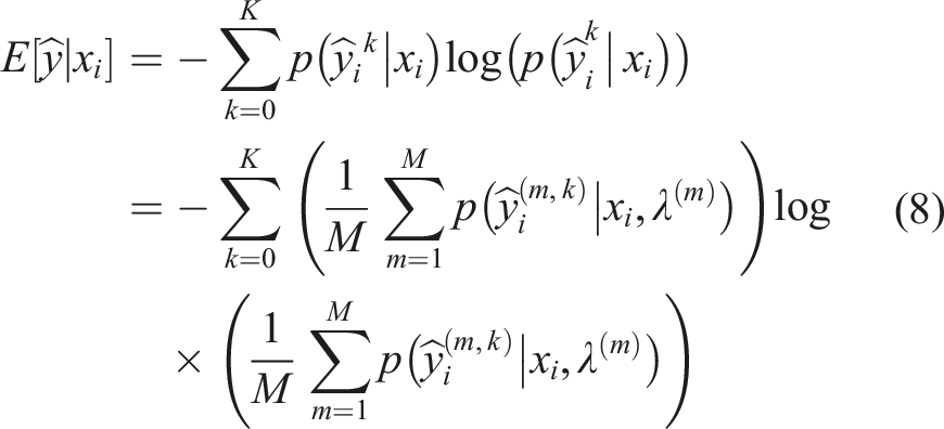
The uncertainty of all diagnostic samples can be measured as the sum of the entropy values of all samples:
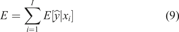
where
The final predicted fault label is
Figure 1 shows a flowchart of the classification framework. Three CNNs, each with convolutional layer kernels of different sizes, are combined using an ensemble approach. The contribution of each classifier to the results is determined using its predicted uncertainty. Dynamic ensemble strategy.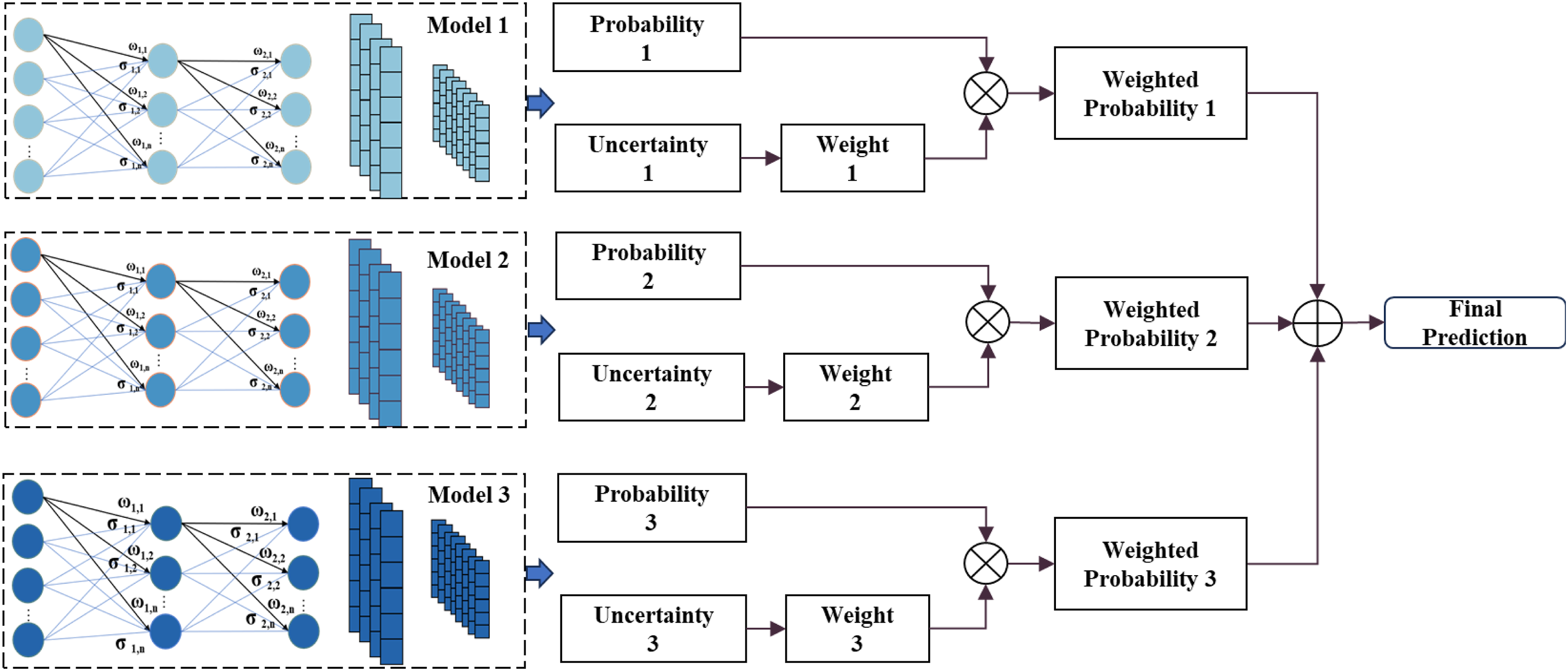
2.4. Proposed structure for fault diagnosis
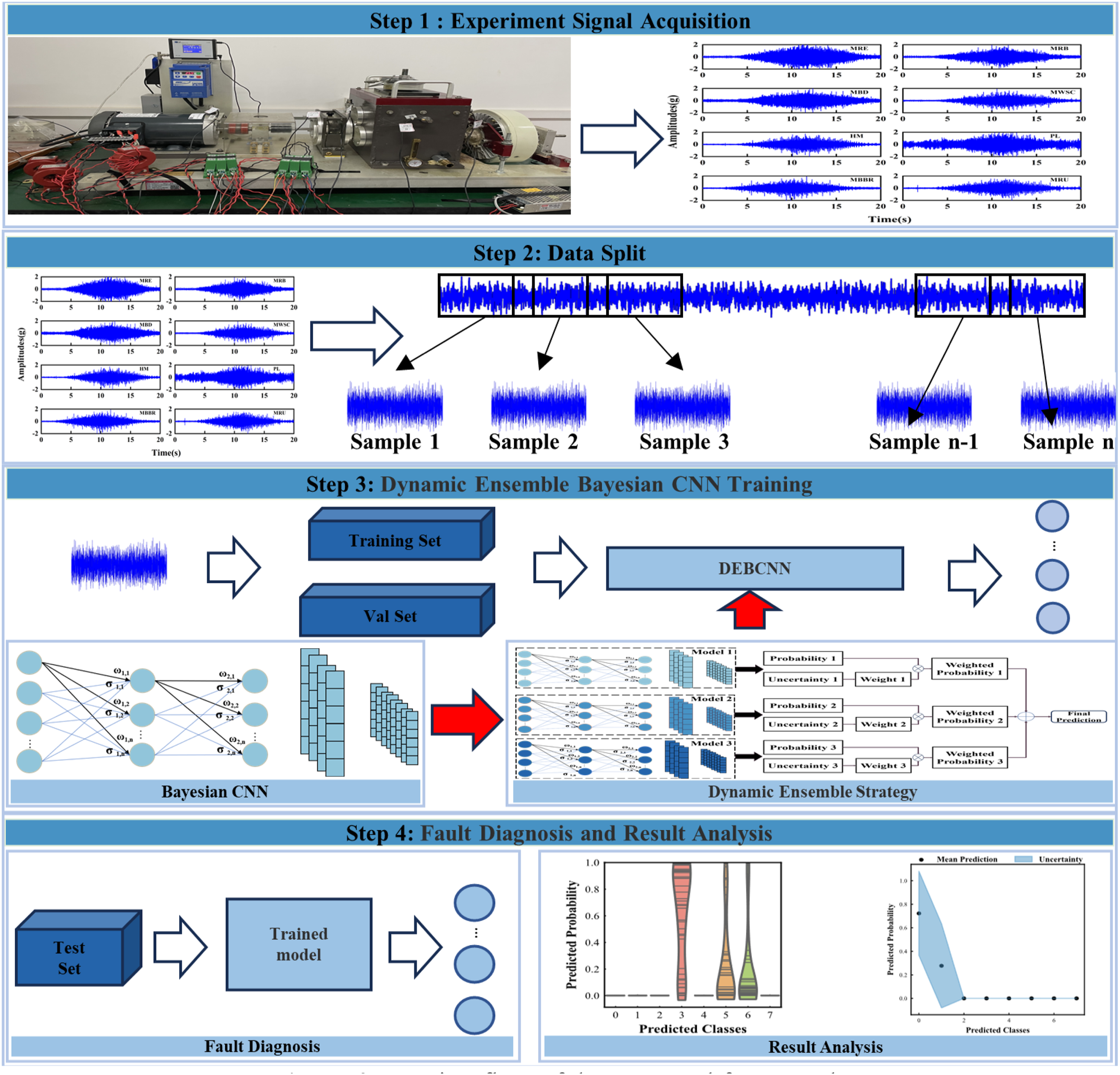
Figure 2 depicts the DEBCNN-based fault diagnosis framework for rotating machinery under time-varying speed conditions. This process consists of four main steps. Step 1: Collect experimental data: The working conditions of the rotating machinery with different types of faults under time-varying speed conditions are simulated to collect vibration signals. Step 2: Data split: Because signals are continuously collected, the continuous working signals are divided into multiple samples of a certain length. Step 3: DEBCNN model training: Using the vibration signal as input, produce the corresponding outputs of each submodel. The contributions of the submodels in the ensemble model are determined based on the uncertainty of their results to complete the model output. Complete the model structure training and save the network parameters using repeated iterative optimization. Step 4: Fault diagnosis and analysis of the results: Based on the saved ensemble model, the predicted probabilities for different fault types finally yield the diagnosis type, providing the corresponding magnitude of uncertainty. Running flow of the proposed framework.
3. Test verification
3.1. Case 1: Motor dataset
3.1.1. Dataset description
The data used in Case 1 were obtained from the laboratory bench shown in Figure 3, which consists of a motor, bearing, gearbox, and brake. Eight different motor health conditions were simulated in the experiment: healthy motor (HM), motor with rotor unbalance (MRU), motor with rotor eccentricity (MRE), motor with rotor bending (MRB), motor with bearing fault (MBF), motor with broken bar (MBB), motor with winding short circuit (MWSC), and motor with voltage imbalance (MVI). The test bench of the motor.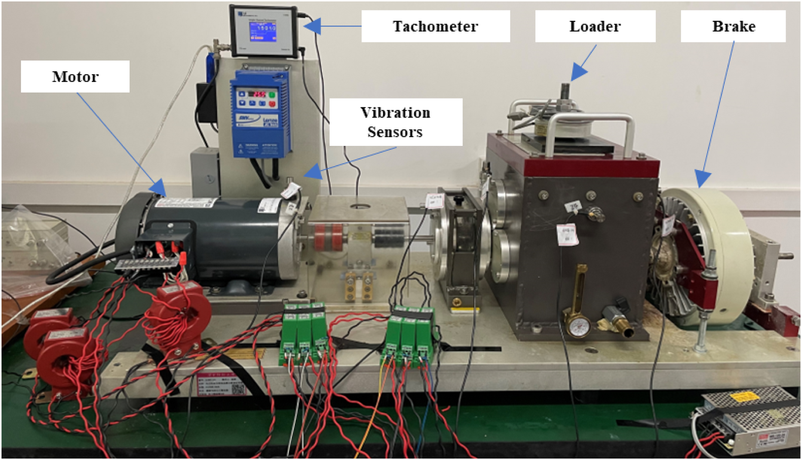
The acceleration sensor continuously sampled the motor-operating signals of different health states for 20 s at a sampling frequency of 25,600 Hz. During this acquisition period, the motor speed was accelerated to 3000 r/min and then decelerated to 600 r/min. Figure 4 shows time-domain graphs of the vibration signals recorded for various motor health states. Given that the gathered vibration data are long time series signals, a sliding segmentation technique was applied to obtain more training samples. A sliding window sampling method was used to divide the original continuous signal into multiple samples. Each sample had a length of 4,096, and the sliding window step was set to 1,024. After sliding segmentation, there were 3,976 samples overall and 497 examples of a single fault type. Vibration signals for the health state of eight different motors under variable speed conditions.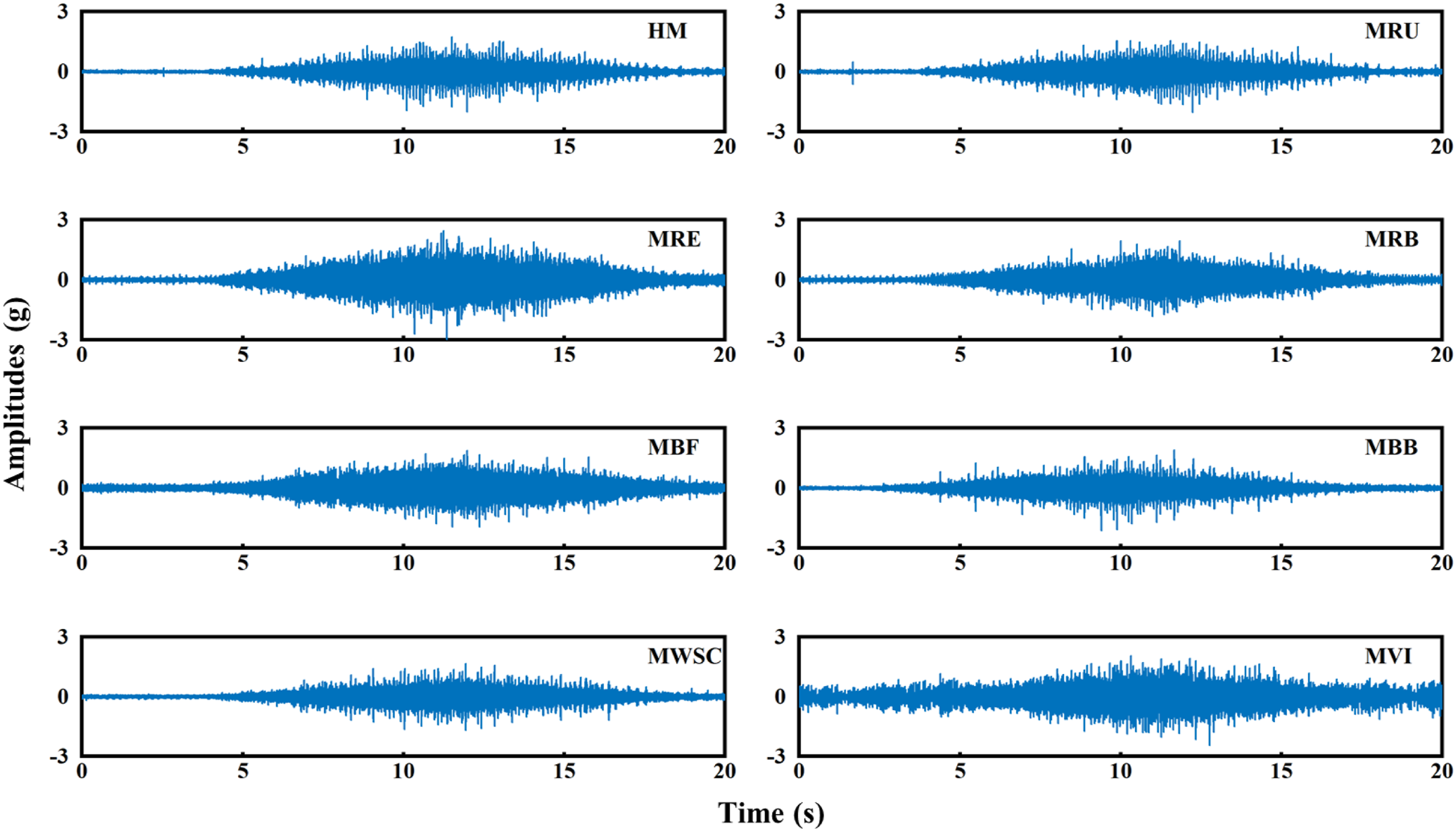
3.1.2. Results and discussion
Various comparative tests were conducted to verify the superiority of the proposed method. The comparison methods included existing multi-scale ensemble strategies and advanced time-varying speed fault diagnosis methods. The different comparison methods are as follows: (1) (2) (3) (4) (5) (6) (7) (8)
The diagnostic accuracy of different diagnostic methods and the variance of multiple experiments are shown in Figure 5. The EMD-MSE-DT method is constrained by parameters such as the number of IMFs in EMD and the scale used for MSE. Furthermore, the DT fault diagnosis model struggles to extract deep fault characteristics, resulting in the lowest performance in terms of accuracy and stability in multi-diagnosis scenarios. In contrast, RP and STFT feature maps effectively capture the distinctive characteristics of various fault types, and the integration of CNNs further enhances fault diagnosis accuracy by leveraging the advantages of two-dimensional (2D) images. The ensemble of multi-scale characteristics within the model significantly improved the precision of the fault diagnosis. Specifically, the combination of the C-CNN, DS evidence theory, and MK-ResCNN achieved a diagnostic accuracy of 98%. The accuracy and stability of multiple diagnoses can be further enhanced by optimizing a multi-scale ensemble strategy. The proposed method employs a dynamic ensemble strategy that adjusts the weights of various scales to adapt to different rotational speeds, thereby reducing the impact of features interfering with the diagnostic results while incorporating multi-scale features.
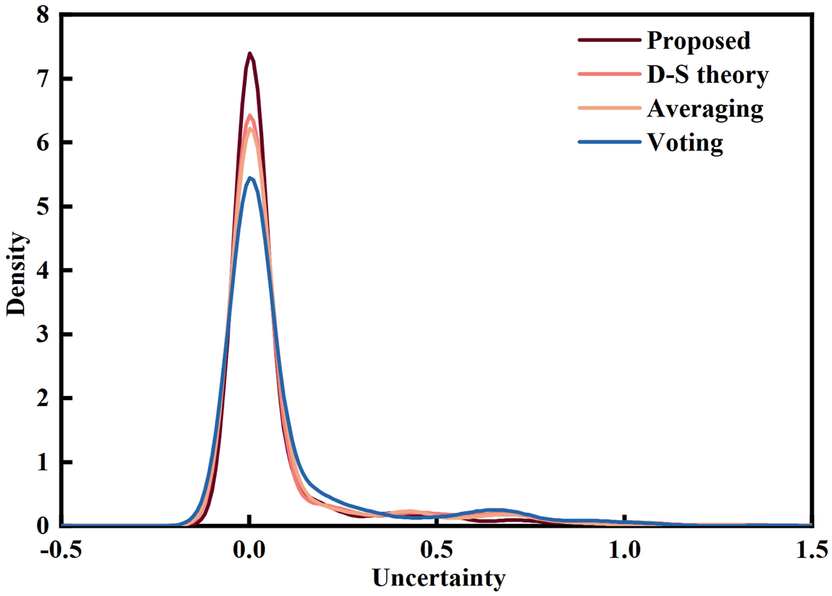
While focusing on the accuracy of diagnostic results, one should also emphasize their reliability. The horizontal coordinate in the Figure 6 indicates the uncertainty of the diagnostic results, and the vertical coordinate represents the density corresponding to the uncertainty. Compared with the other three strategies, the uncertainty of the proposed ensemble strategy is closer to zero. Under time-varying speed conditions, the difference in fault characteristics of the same fault type owing to varying speeds directly leads to uncertainty in the diagnostic results. A concentration of uncertainty near zero suggests a large gap between the probabilities of the correct and incorrect labels in the prediction results, thereby reducing the probability that the current diagnosis is incorrect. Consequently, the accuracy of the diagnostic results and the reliability of the corresponding results across multiple experiments improve. Diagnostic results of the proposed method and the comparison method: (a) accuracy and (b) variance. Comparison of the proposed method with the uncertainty of the diagnostic results of existing ensemble strategies.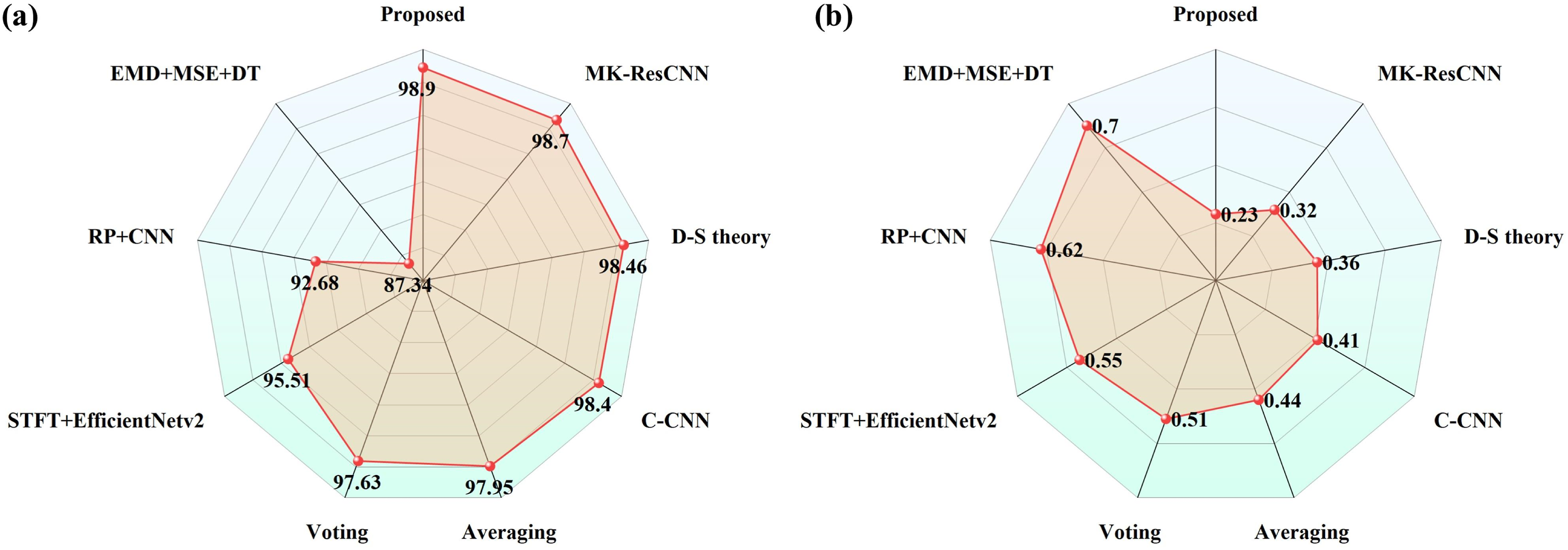
3.1.3. Anti-noise performance test
To evaluate the performance of the proposed method, different levels of Gaussian white noise were randomly added to the raw signals of motors with various fault types. The magnitude of background noise is typically measured using the signal-to-noise ratio (SNR), which is defined as the ratio of the useful signal power to the noise power in the signal and is expressed in decibels (dB).
The results are shown in Figure 7. As the noise in the signal increases (SNR gradually decreases), the complexity of the signal gradually increases, and the original signal features are submerged, making it more difficult for the diagnostic model to extract fault features. However, the proposed method consistently achieves stable diagnostic results under different noise conditions, and the diagnostic accuracy of the DEBCNN remains close to 97% even at SNR = −6 dB. Diagnostic accuracy of the DEBCNN model on the motor dataset under different noise conditions.
To further compare the adaptability of different scale models under noisy conditions, single-scale, two-scale, three-scale, and four-scale models were built by setting up networks with convolutional kernel sizes of 3, 5, 7, and 9, respectively, and tested at SNR = −2 dB. The t-distributed stochastic neighbor embedding (T-SNE) results for the test sets of different models are shown in Figure 8. Compared with the multi-scale model, the single-scale model struggles to distinguish each fault type effectively. As the scale increases, the degree of differentiation among different fault types improves, as shown in Figure 8(c), where the fault types are well differentiated and the overlap between fault categories is reduced. Even in noisy environments, the three-scale ensemble model achieved diagnostic results similar to those under the five-noise condition. Increasing the number of scale features did not improve the ability of the model to discriminate between different fault types. Instead, the time required for the diagnostic process increases. Therefore, a three-scale dynamic ensemble model was used in this study. The t-distributed stochastic neighbor embedding (T-SNE) visualization results of different scale models: (a) single-scale; (b) two-scale; (c) three-scale; (d) four-scale.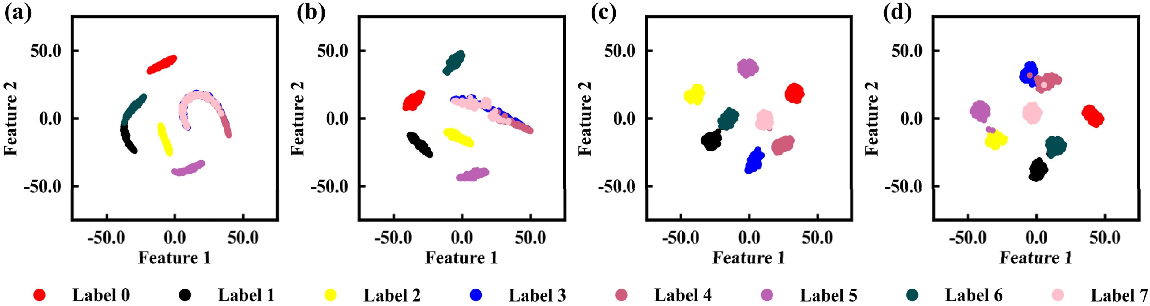
3.2. Case 2: Bearing dataset
3.2.1. Dataset description
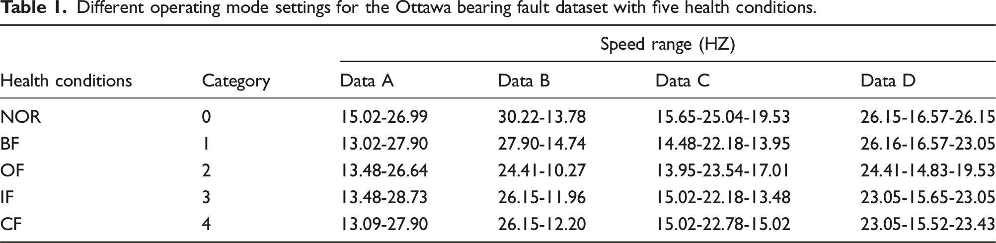
The University of Ottawa time-varying speed bearing fault dataset was gathered on an experiment bench, as shown in Figure 9 (Huang and Baddour, 2018). The motor powers the shaft, while the AC drives, controls, and adjusts its speed. The healthy and experimental bearings, both of type ER16 K, support the left and right sides of the shaft. Various experimental bearings were changed to simulate multiple health states, including the normal state (NOR), ball fault (BF), outer ring fault (OF), inner ring fault (IF), and mixed fault (MF) containing the above three fault types. The vibration signals of the experimental bearing at various health stages were recorded using an accelerometer (Type 623C01) at 200 KHz. The shaft speed is measured using incremental encoders. Within 10 s, the experimental bearings in various health stages finished simulating time-varying rotational speeds; hence, the accelerometers continually recorded vibration signals for 10 s. Bearing test platform of Ottawa University.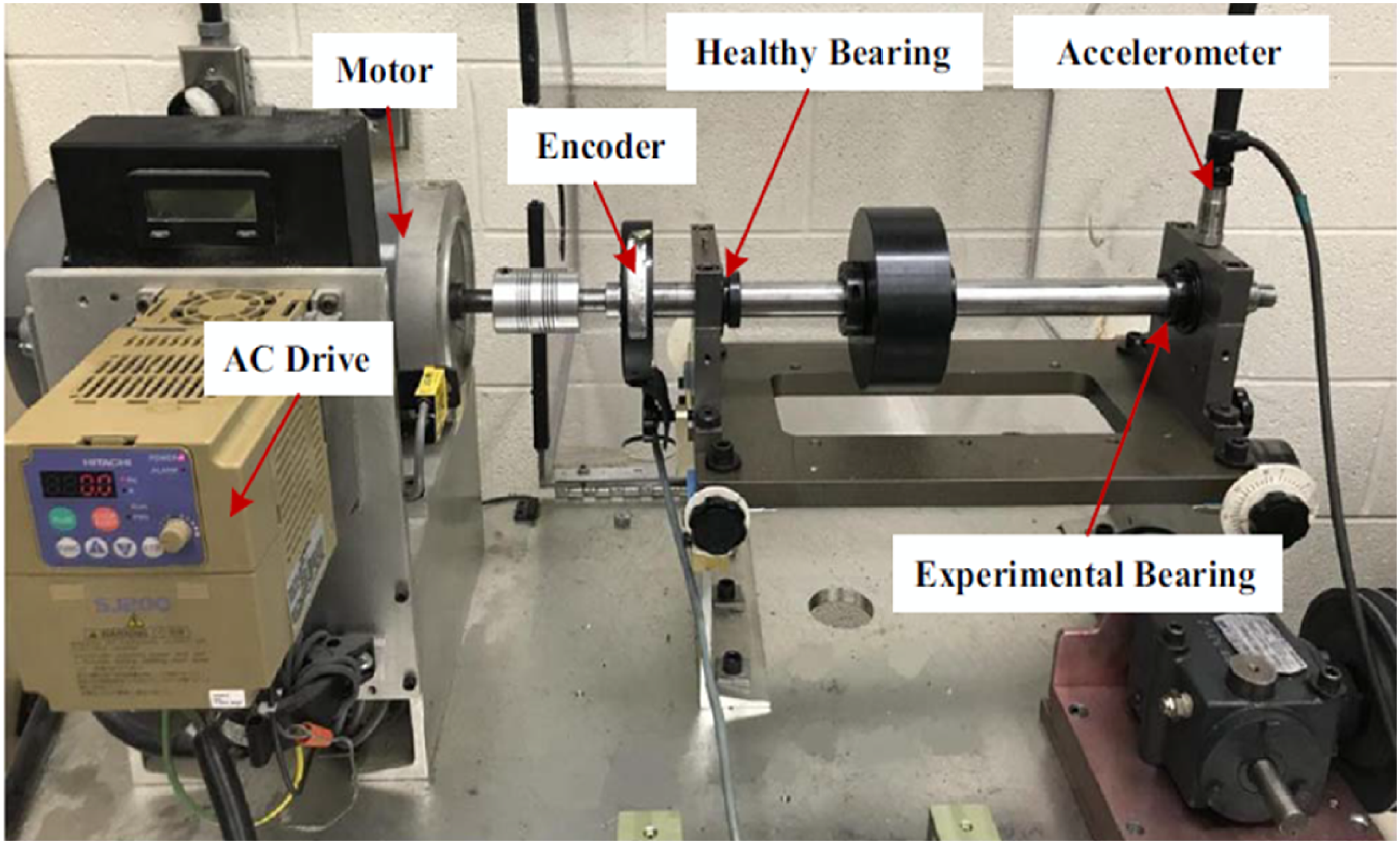
Different operating mode settings for the Ottawa bearing fault dataset with five health conditions.
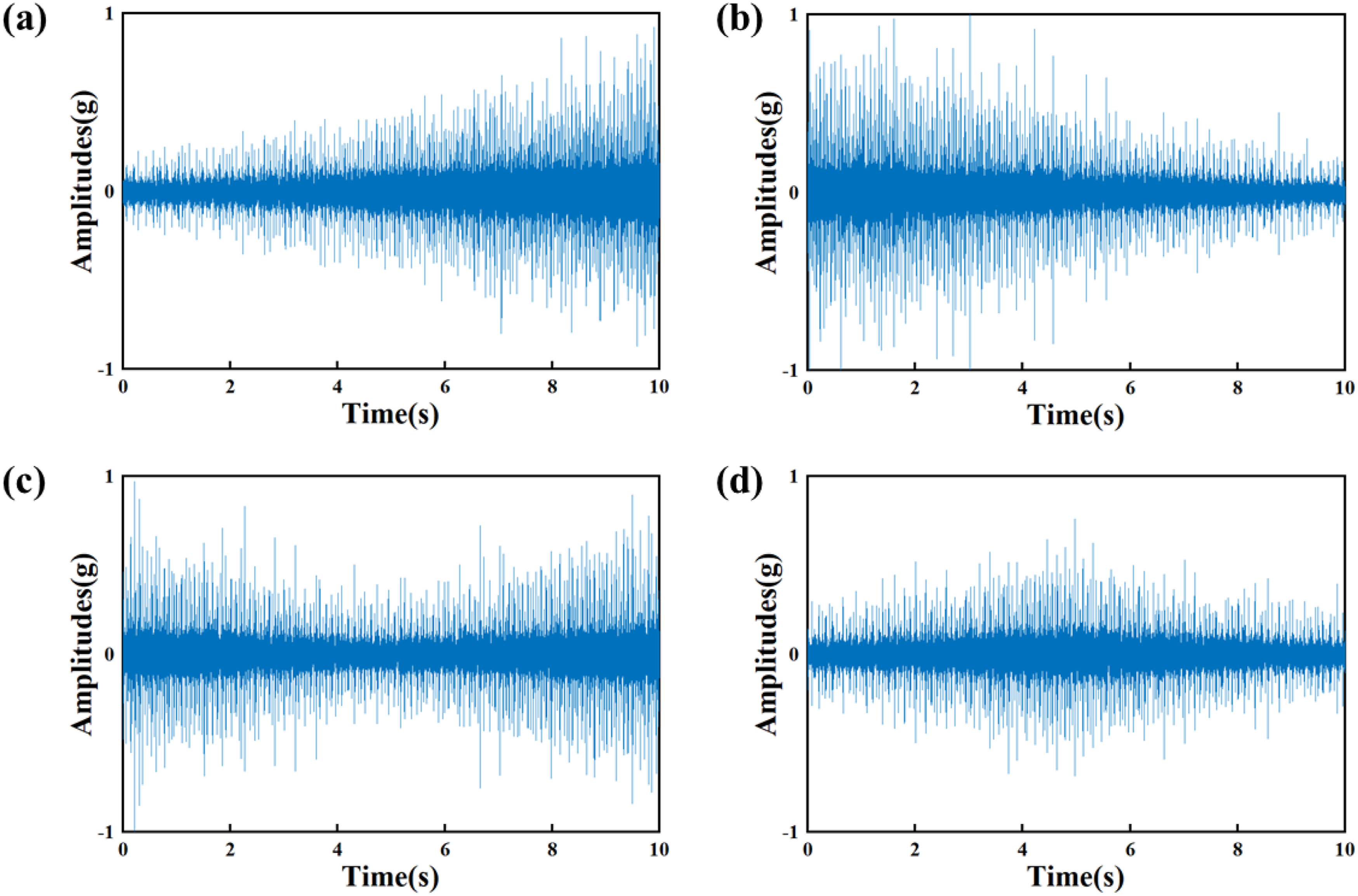
Time-domain diagrams of normal-state bearings under four variable-speed conditions: (a) acceleration, (b) deceleration, (c) acceleration and then deceleration, and (d) deceleration and then acceleration.
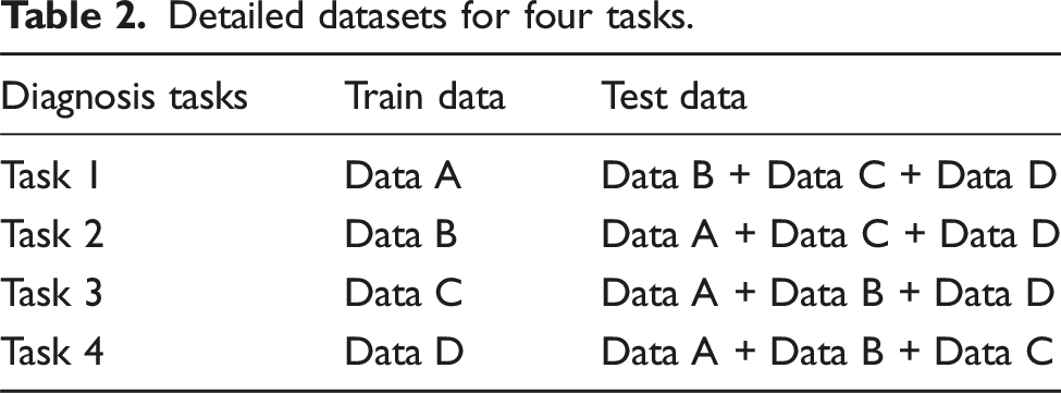
Detailed datasets for four tasks.
3.2.2. Results and discussion
The diagnostic accuracies of the proposed method and eight comparison methods for the four tasks are shown in Figure 11. Each method executed 10 diagnostic tests for different tasks to obtain the final average accuracy and variance. Diagnostic results of the proposed and compared methods in four tasks: (a) accuracy and (b) variance.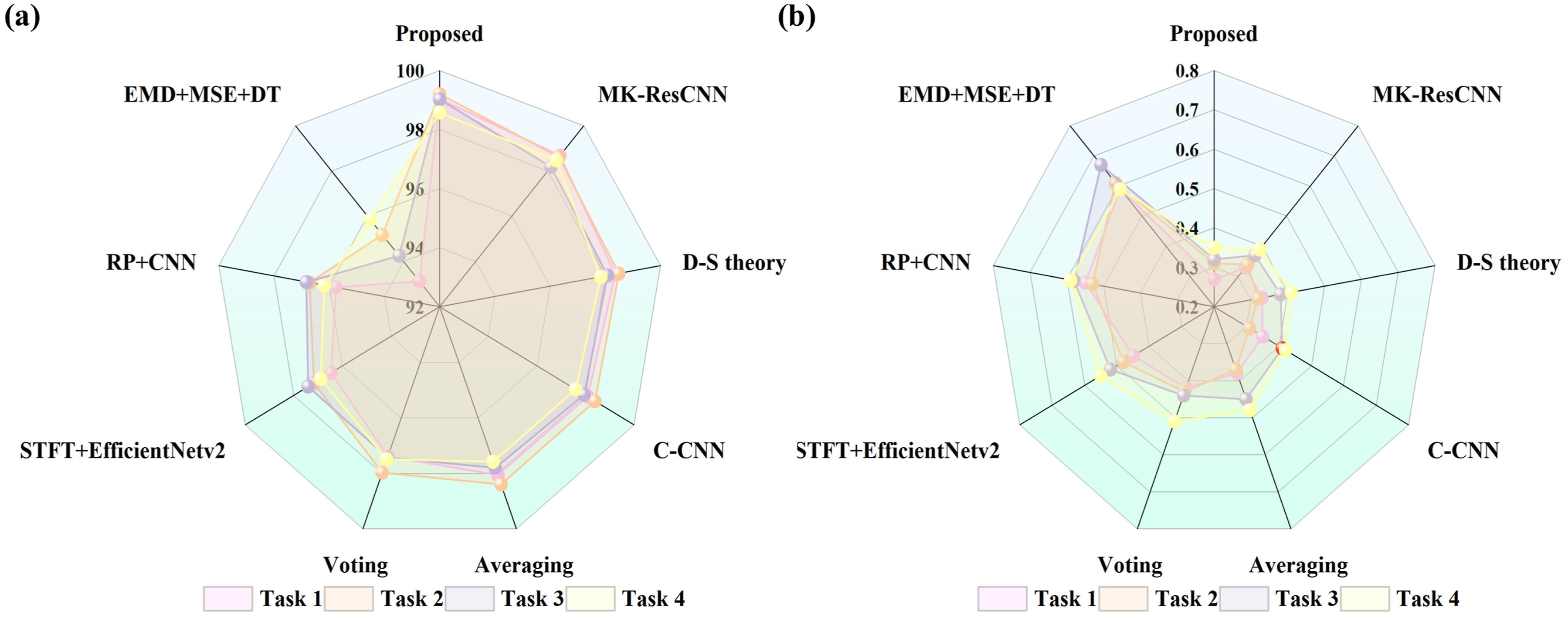
Compared with the motor dataset, although the bearing dataset had only five fault types, different time-varying speed working conditions were added. On the one hand, the difference between the acceleration and deceleration work process types increases the variance between the data used for model training, which makes it more difficult to extract fault features. On the other hand, owing to the differences in the data distribution during the testing of other work process data, the fault features extracted by the model during the testing phase further affect the effectiveness of the fault diagnosis. Because of its ability to filter relevant features from different resolution features and reduce interfering features, the proposed method provides higher diagnostic accuracy than other state-of-the-art fault diagnosis methods under time-varying speeds and multiple work process conditions. The superiority of the proposed strategy is further demonstrated by the volatility of multiple experimental results, with lower volatility indicating that the proposed method can effectively reduce the impact of different acceleration and deceleration processes on the diagnostic results.
Regarding the uncertainty of the diagnostic results, the ensemble results of the proposed ensemble strategy were close to zero for all four diagnostics tasks, as shown in Figure 12. For task b, the accuracies of the averaging and voting ensembles were 98.41% and 97.97%, respectively. However, the distribution of uncertainty for these two results is close to the same, which suggests that although the average ensemble has higher accuracy in general, there is a phenomenon similar to voting when it comes to a single experiment, because the voting ensemble is similar to struggling between the correct and wrong fault types, with insufficient confidence in the diagnostic results. The diagnostic accuracy reflects the proportion of correct fault types in all sample diagnostic results, whereas the uncertainty demonstrates the confidence of a particular diagnostic result in the model. The high accuracy and low uncertainty of the proposed ensemble strategy indicate that the model is stable, reliable, capable of making safe and accurate predictions in most cases, and effective in reducing the impact of time-varying speed on fault diagnostic results. Uncertainty distribution of the diagnostic results of the proposed ensemble and comparison strategies in the four diagnostic tasks.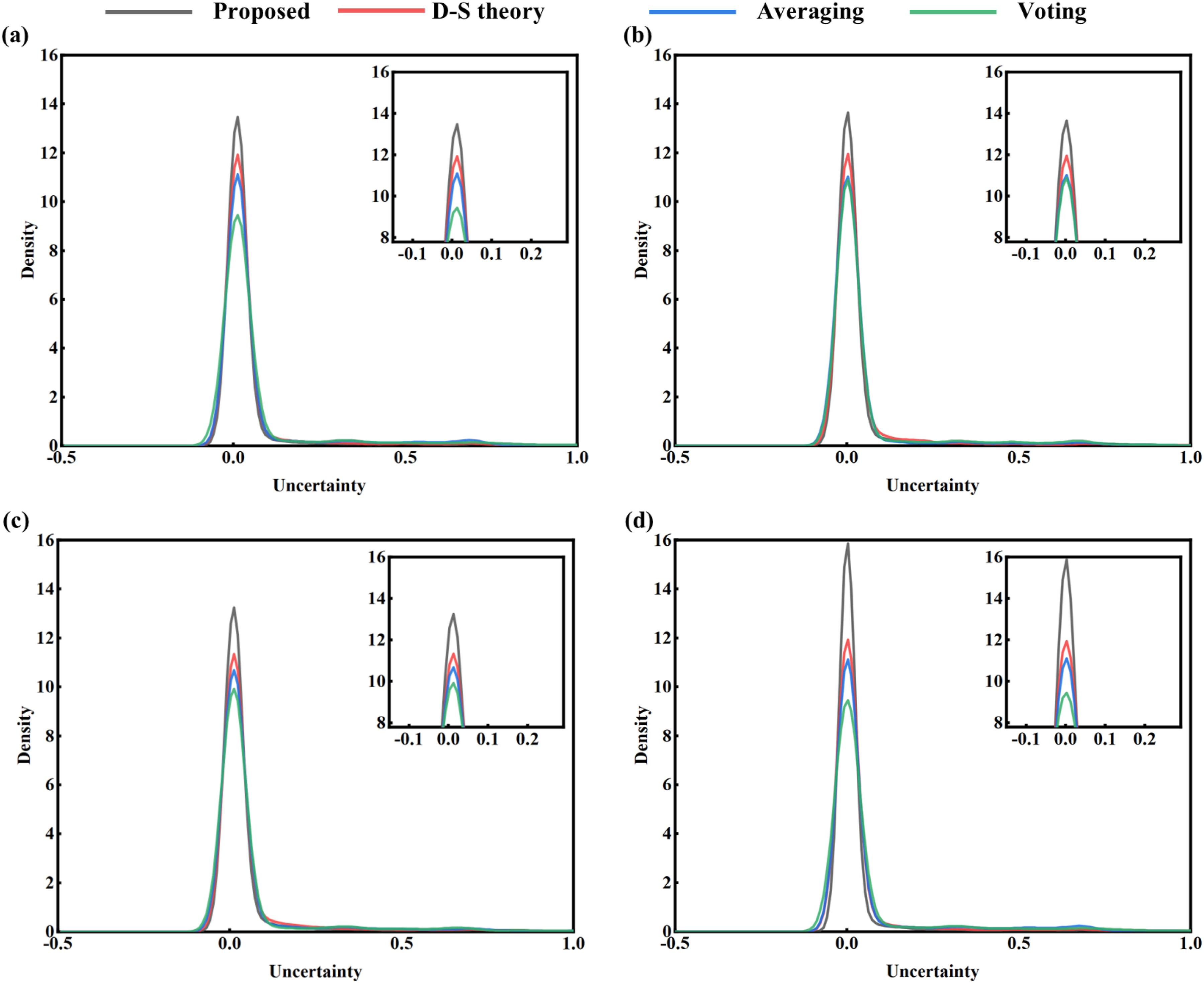
3.2.3. Anti-noise performance test
Simulated interference noise with an SNR of −2 dB is added to the original signals of the four tasks; then the anti-noise interference performance of the DEBCNN model is tested in each of the four tasks. The DEBCNN achieved diagnostic accuracies of 98.72%, 98.74%, 98.28%, and 98.22% in the four noise-containing diagnostic tasks, as shown in Figure 13, and the diagnostic accuracies were close to those of the tasks with no noise added, indicating that the DEBCNN model has good noise resistance. The presence of noise further increases the difference in the effectiveness of multi-scale features in the task of diagnosing fault types; therefore, it is necessary to reduce the influence of interference features on the final diagnostic results and increase the weight of useful features when fusing multi-scale features using the dynamic ensemble strategy, which ensures that the influence of the noise interference component is reduced while combining multi-scale features. Diagnostic accuracy of the DEBCNN model under different noise conditions. T-SNE visualization results of different scale models in four tasks: (a) Task 1, (b) Task 2, (c) Task 3, and (d) Task 4.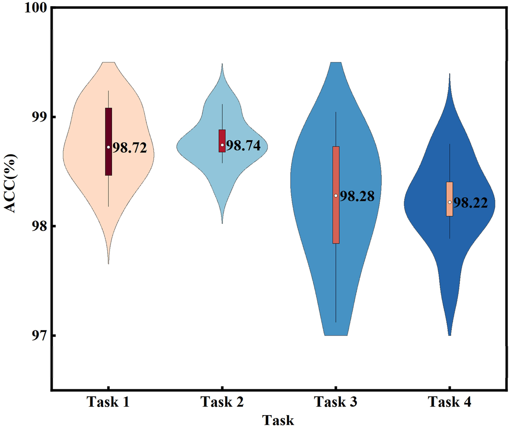
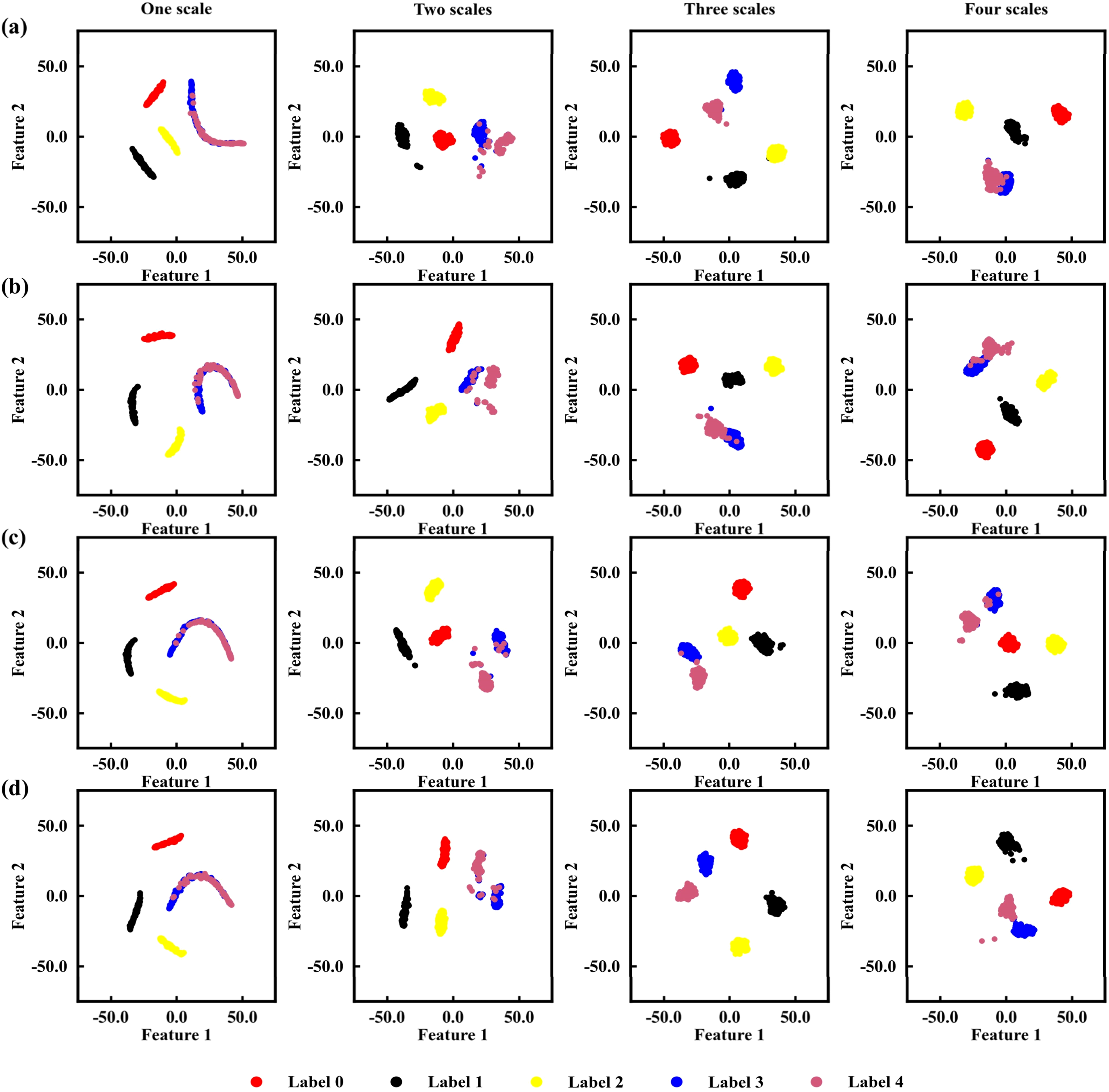
From the T-SNE results in Figure 14, it can be observed that the multi-scale model had better noise resistance than the single-scale model for the four diagnostic tasks of the bearing dataset. Additionally, the diagnostic accuracies of the single-scale, two-scale, three-scale, and four-scale models were 93.83%, 95.67%, 98.72%, and 98.69%, respectively, for Task 1. It was difficult to distinguish the fault type composite faulty bearing and inner ring faulty bearing for the single-scale and two-scale models, whereas the three-scale model significantly improves this problem, reduces the misdiagnosis rate between different faults, and improves the accuracy of fault diagnosis. There is a certain coupling relationship between the inner ring fault and the composite fault, and it is difficult to extract the fault characteristics from a single scale only to achieve effective differentiation. The combination of different scale characteristics can improve the degree of differentiation of similar fault types.
4. Conclusion
This study proposes a dynamic ensemble strategy based on uncertain driving for the fault diagnosis of rotating machinery under time-varying speed conditions. Based on the principle of a BCNN, the uncertainty of the fault diagnosis results under time-varying speed conditions was measured. The robustness of the prediction results was improved through multi-scale features, and the uncertainties of different features were further used to determine their weights in the ensemble framework. This method can remove speed-sensitive features and retain fault features, thereby ensuring the reliability of the fault diagnosis results under time-varying speed conditions. The analysis results verified the effectiveness of the proposed strategy, and compared with traditional ensemble strategies, the proposed method has advantages in terms of diagnostic accuracy and corresponding uncertainty.
Future work will explore the performance of this methodology under multi-component coupled faults and small sample conditions.
Footnotes
Acknowledgments
The authors thank the editors and anonymous reviewers for their helpful comments.
Declaration of conflicting interests
The author(s) declare no potential conflicts of interest with respect to the research, authorship, and/or publication of this article.
Funding
The author(s) disclose the receipt of the following financial support for the research, authorship, and/or publication of this article: This work was supported by the National Natural Science Foundation of China (51879056) and the Shandong Provincial Natural Science Foundation (ZR2023QE009). The author also thanks the mentor for suggesting changes to the content of the paper.