Screw dynamics modeling of parallel robots and its hyperbolic convergence law sliding mode control strategy

Abstract

This study introduces a method to establish the dynamic model of a parallel robot using screw theory and the d’Alembert-Lagrange equation. Based on this model, a robust sliding mode control strategy utilizing hyperbolic convergence laws is proposed. The d’Alembert-Lagrange equation and screw theory are employed to construct a concise dynamic equation for the parallel robot, making it more suitable for control applications. Additionally, a formula for directly calculating the inertial wrench is presented. To achieve precise control, a sliding mode control strategy with double hyperbolic convergence law is implemented to ensure chattering-free performance. A novel double hyperbolic convergence law disturbance observer is designed to estimate unmodeled dynamics and uncertain disturbances, enhancing the system’s robustness. The control strategy is validated through numerical simulations, demonstrating significant improvements in chattering-free performance, tracking accuracy, and tracking speed.

Keywords

Parallel robot screw theory D’Alembert-Lagrange equation robot dynamics sliding mode control double hyperbolic convergence law

1. Introduction

In the rapidly evolving fields of automation and intelligent manufacturing, parallel robots—a high-performance mechanical system—are gaining prominence due to their unique advantages and broad application prospects. These robots feature multiple closed-loop motion links, providing them with high rigidity, accuracy, and dynamic response (Dong et al., 2021; Gosselin, 1995; Merlet, 2005). In particular, they excel in specific tasks, particularly in scenarios demanding high speed, load capacity, and repetitive positioning accuracy.

Parallel robots commonly operate at high speeds, posing a critical challenge: achieving precise control (Wu et al., 2021). High-precision motion control is inherently demanding (Li and Wu, 2004). Firstly, the inherent structure of parallel robots results in strong coupling between their kinematics and dynamics (Cheng et al., 2022). Modeling the nonlinear dynamics of parallel robots presents considerable difficulty (Abo-Shanab, 2020). Secondly, accounting comprehensively for time-varying perturbations and unmodeled dynamics remains elusive, hindering the attainment of sufficient control accuracy.

Traditionally, researchers have employed several methods to analyze the dynamics of parallel robots, including the Newton-Euler method (Do and Yang, 1988), Lagrange method (Asker et al., 2014), and the virtual work principle (Tsai, 1999a). Additionally, some scholars have used bond graph theory (Bidard, 1993; Guo et al., 2015) to construct the multi-energy domain dynamics model of parallel robots. Newton-Euler method as a classical mechanics method, there is a need for multiple iterations and the existence of a large number of intermediate forces, which is too cumbersome for the dynamics solution of the control model. In addition to the Newton-Euler method, the rest of the Lagrange method, the method of the principle of virtual work, and the bonding diagram method are all energy-based methods, which are more suitable for the construction of the complex multi-body dynamics model. The screw theory is an effective tool to study the dynamics of space bodies (An et al., 2017; Chen et al., 2017; Cibicik and Egeland, 2019); Bidrard proposed the concept of screw bond graph in 1993 (Bidard, 1993), Guo et al. (2015) successfully applied the screw bond graph to the dynamics of parallel robots; Gallardo and Cheng combined the screw theory and the virtual work principle of dynamics to study the dynamics of manipulators (Cheng et al., 2022; Gallardo et al., 2003; Gallardo-Alvarado et al., 2008, 2018). In general, a spatial mechanism has six degrees of freedom, and the Plücker coordinates of the screw also have six variables (Qiu et al., 2021). This correspondence is advantageous for constructing a simpler and more concise process for solving dynamics.

Traditional computational torque control is effective when the robot’s dynamics are fully and accurately modeled. However, its control accuracy significantly degrades in the presence of large unmodeled dynamics and disturbances (Kardos, 2019; Xiao et al., 2024). Feedforward PD control partially mitigates disturbances but relies on high modeling accuracy. Neural network techniques can enhance the robustness of parallel robotic systems by identifying and compensating for uncertainties, but this approach demands extensive training data, computational resources, and cost, and lacks explicit stability proofs (Nguyen and Cheah, 2022). Sliding mode control, which employs a nonlinear switching function, quickly steers the system state toward the desired sliding surface even in the presence of perturbations, demonstrating robustness (Li et al., 2022). Although sliding mode control effectively handles unmodeled dynamic perturbations, the issue of high-frequency jitter in traditional sliding mode control limits its practical applicability (Levant, 1993).

In this paper, we construct a dynamics model for a robot using screw theory and the d’Alembert-Lagrange equations. Based on this model, we investigate a sliding mode control strategy for parallel robots employing hyperbolic convergence law. The paper introduces an innovative approach in two key areas. First, it presents a concise formula for directly calculating spatial inertia force using screw notation. This simplifies the calculation process and enables a concise and unified kinematics-to-dynamics modeling using screw. Secondly, we design a novel high-precision, vibration-free sliding-mode controller for parallel robots. Additionally, a sliding-mode disturbance observer is developed to address high-frequency vibration issues. The observer enhances system robustness by compensating for uncertainty. The paper proceeds as follows: In Section 2, we establish the full Jacobi matrix of the parallel robot using the dual space and closed-loop vector method. In Section 3, we construct the robot dynamics model using screw theory and the d’Alembert-Lagrange equations. We introduce a formula for calculating the inertial wrench related to the moving platform. Section 4 details the design of a combined hyperbolic convergence law sliding-mode controller (HCLSMC) and an expanded sliding-mode observer for the parallel robot control strategy. In Section 5, we simulate and verify the controller’s advantages in terms of accuracy, tracking speed, chattering-free control, and interference immunity. Finally, Section 6 presents the paper’s conclusions.

2. Kinematic modeling

2.1. Kinematic inverse solution

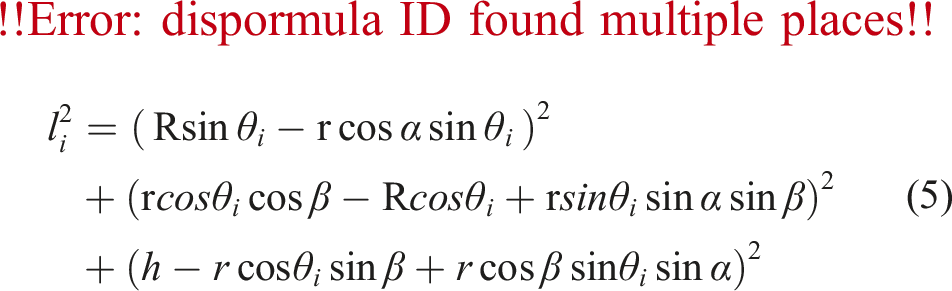
Kinematic analysis forms the fundamental groundwork for parallel robots. It serves as the foundation for velocity, acceleration, force, and dynamics analyses. This paper focuses on studying the robust control algorithm for parallel robots. Consequently, we establish only the inverse kinematics model for the parallel robot. Unlike tandem robots, the inverse kinematics of parallel robots are relatively straightforward to construct. We compute the inverse kinematics using the traditional closed-loop vector method, which efficiently relates the working end position to the driving position.

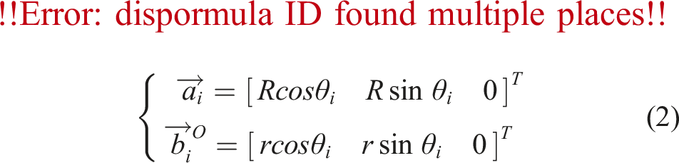
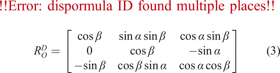
For the 3UPS/PU parallel robot shown in Figure 1, the Hook hinge node between the bottom base and the side chain i is marked as A_i, the ball hinge on the side chain i is marked as B_i, the intersection point of the PU kinematic chain and the plane A₁A₂A₃ is noted as point D, and the center point of Hook hinge of the movable platform connecting to the PU kinematic chain is noted as point O. The base coordinate system is established with the origin of the point D, and the direction of the vector $\vec{D A}$ and the vector $\vec{D O}$ are the positive direction of x and z axes respectively, and the positive direction of the y-axis is determined by the right-hand rule. At the initial pose, a coordinate system {O} is established at point O, parallel to the {D} coordinate system and rigidly attached to the end-effector platform. Its PU kinematic chain constrains its movement along the x-axis and y-axis and rotation around the z-axis, and the chain A_iB_i can provide all six degrees of freedom, so the robot has three degrees of freedom. The closed-loop vector diagram is shown in Figure 2.

{\vec{a}}_{i} + l_{i} {\vec{s}}_{3}^{i} = h {\vec{s}}_{3}^{4} + R_{O}^{D} {\vec{b}}_{i}^{O} (i = 1,2,3)

(1)

where

{\vec{s}}_{3}^{i}

is the unit vector pointing from point A_i to point B_i,

{\vec{s}}_{3}^{4}

is the unit vector pointing from point D to point O,

{\vec{a}}_{i}

is the vector pointing from point D to point A_i,

{\vec{b}}_{i}

is the vector pointing from point O to point B_i, l_i is the length of

\vec{A_{i} B_{i}}

, h is the length of

\vec{O D}

\{\begin{cases} {\vec{a}}_{i} = & {[\begin{matrix} R c o s θ_{i} & R \sin θ_{i} & 0 \end{matrix}]}^{T} \\ {\vec{b}}_{i}^{O} = & {[\begin{matrix} r c o s θ_{i} & r \sin θ_{i} & 0 \end{matrix}]}^{T} \end{cases}

(2)

R_{O}^{D} = [\begin{matrix} \cos β & \sin α \sin β & \cos α \sin β \\ 0 & \cos β & - \sin α \\ - \sin β & \cos β \sin α & \cos α \cos β \end{matrix}]

(3)

θ_{i} = \frac{2 (i - 1)}{3} π, (i = 1,2,3)

(4)

where R and r are the radii of the fixed base and the moving platform, respectively.

R_{O}^{D}

is the rotation matrix from coordinate system {O} to coordinate system {D}, and α and β are the angles of rotation of the moving platform around the x-axis and y-axis of the coordinate system {D}, respectively.

\begin{aligned} l_{i}^{2} & = {(\begin{matrix} R \sin θ_{i} - r \cos α \sin θ_{i} \end{matrix})}^{2} \\ + {(r c o s θ_{i} \cos β - R c o s θ_{i} + r s i n θ_{i} \sin α \sin β)}^{2} \\ + {(h - r \cos θ_{i} \sin β + r \cos β \sin θ_{i} \sin α)}^{2} \end{aligned}

(5)

Figure 1.

The 3UPS/PU parallel robot model.

Figure 2.

Closed loop vector diagram.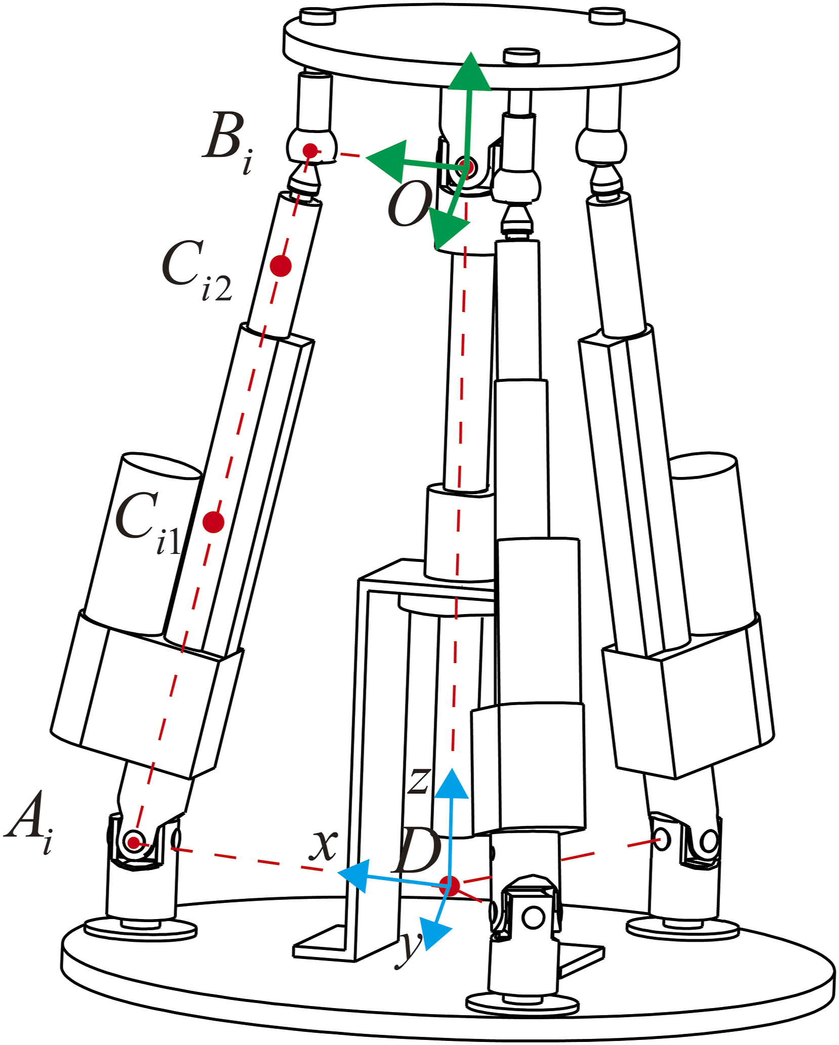

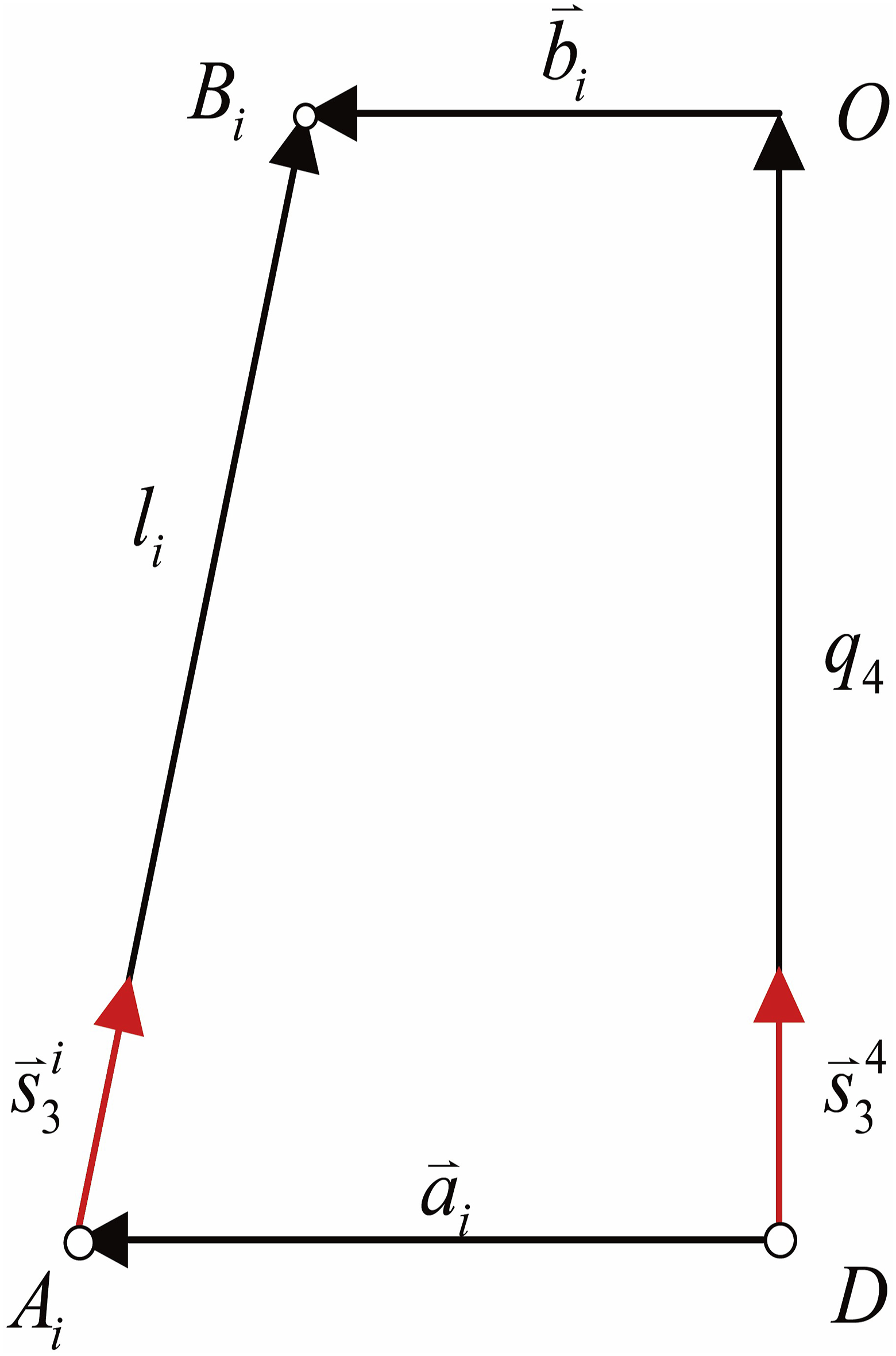
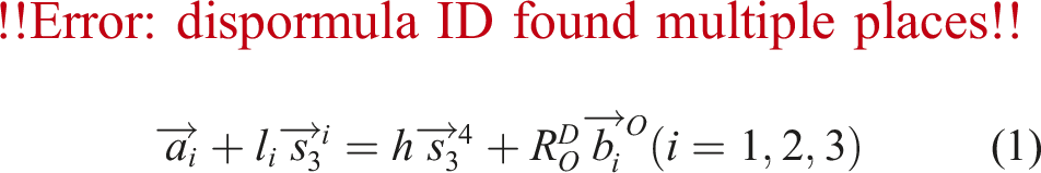
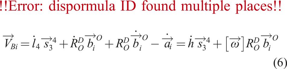
Differentiating Equation (1) with respect to time yields the velocity of point B_i as:

{\vec{V}}_{B i} = {\dot{l}}_{4} {\vec{s}}_{3}^{4} + {\dot{R}}_{O}^{D} {\vec{b}}_{i}^{O} + R_{O}^{D} {\dot{\vec{b}}}_{i}^{O} - {\dot{\vec{a}}}_{i} = \dot{h} {\vec{s}}_{3}^{4} + [\vec{ω}] R_{O}^{D} {\vec{b}}_{i}^{O}

(6)

where,

[\vec{ω}] = [\begin{matrix} 0 & 0 & ω_{O y} \\ 0 & 0 & - ω_{O x} \\ - ω_{O y} & ω_{O x} & 0 \end{matrix}], ω_{O x} = \dot{α}, ω_{O y} = \dot{β}

(7)

The relationship between

{\vec{V}}_{b}

and the rotational angular velocity

{\vec{ω}}_{i}

\vec{A_{i} B_{i}}

is:

{\vec{V}}_{B i} = {\dot{l}}_{i} {\vec{s}}_{3}^{i} + l_{i} [{\vec{ω}}_{i}] {\vec{s}}_{3}^{i}

(8)

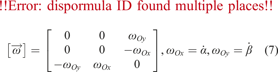
Fork multiplication operation with ${\vec{s}}_{3}^{i}$ on both sides of equation (8) at the same time, from the relationship between ${\vec{s}}_{3}^{i} \cdot {\vec{s}}_{3}^{i} = 1$ and ${\vec{s}}_{3}^{i} \times {\vec{s}}_{3}^{i} = 0$ , we can get the relationship between each side of the parallel robot branch chain has a rotation angular velocity of:

{\vec{ω}}_{i} = \frac{({\vec{s}}_{3}^{i} \times {\vec{V}}_{B i})}{l_{i}}

(9)

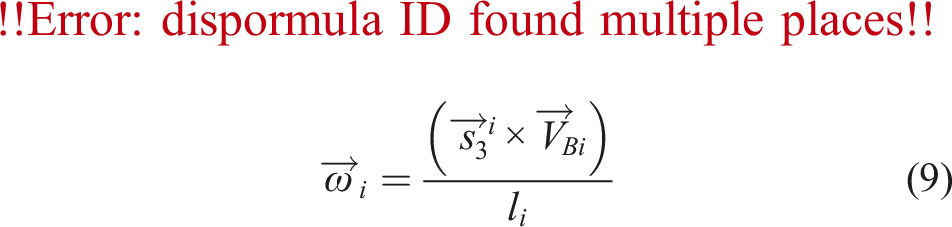
The angular acceleration ${\dot{\vec{ω}}}_{i}$ of the side chain can be obtained by the derivation of Formula (9) to time:

{\dot{\vec{ω}}}_{i} = - \frac{1}{l_{i}^{2}} ({\vec{s}}_{3}^{i}) + \frac{1}{l_{i}} [({\vec{ω}}_{i} \times {\vec{s}}_{3}^{i}) \times {\vec{V}}_{B i} + {\vec{s}}_{3}^{i} \times {\dot{\vec{V}}}_{B i}]

(10)

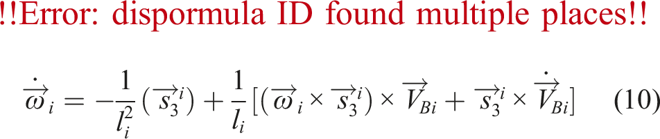
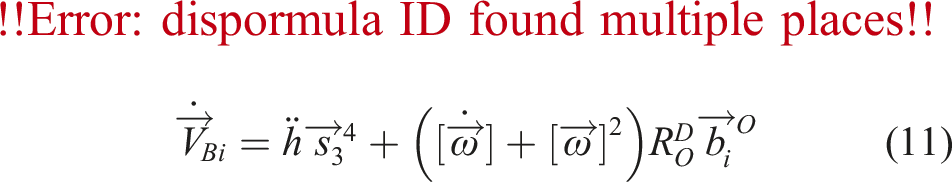
Taking the first derivative of equation (6) with respect to time, we can obtain the acceleration at point B_i:

{\dot{\vec{V}}}_{B i} = \ddot{h} {\vec{s}}_{3}^{4} + ([\dot{\vec{ω}}] + {[\vec{ω}]}^{2}) R_{O}^{D} {\vec{b}}_{i}^{O}

(11)

From the closed-loop vector method, the positions of the center of mass C_i1 of the lower linkage of A_iB_i and the center of mass C_i2 of the upper linkage of A_iB_i can be calculated as:

\{\begin{cases} {\vec{D C}}_{i 1} = {\vec{D A}}_{i} + l_{ci1} {\vec{s}}_{3}^{i} \\ {\vec{D C}}_{i 2} = {\vec{D A}}_{i} + (l_{i} - l_{ci2}) {\vec{s}}_{3}^{i} \end{cases}

(12)

where l_ci1 is the length between the center of mass C_i1 of the lower link of A_iB_i and the point A_i, and l_ci2 is the length between the center of mass C_i2 of the upper link of A_iB_i and the center of the ball hinge B_i.

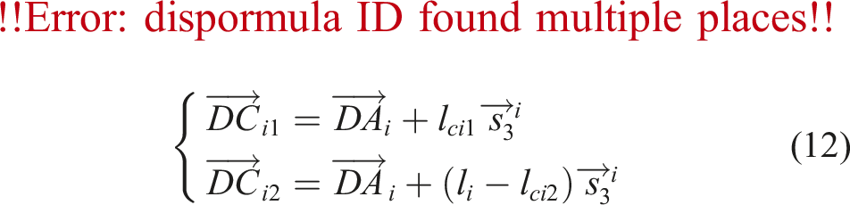
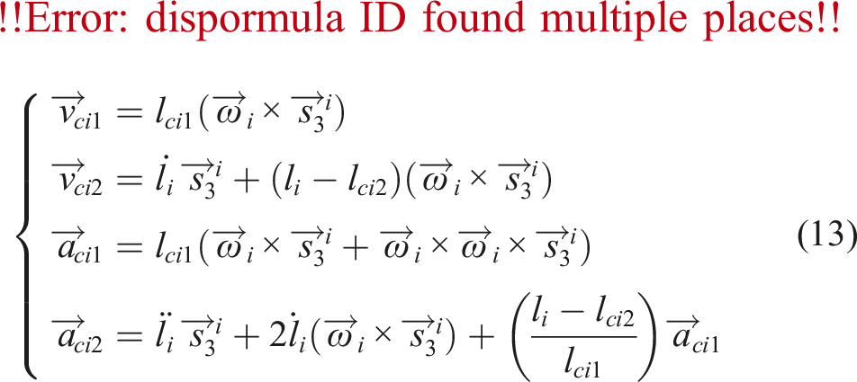
From equation (12), the velocities and accelerations of the lower link centroid C_i1 and the upper link centroid C_i2 of A_iB_i can be calculated as follows:

\{\begin{cases} {\vec{v}}_{ci1} = l_{ci1} ({\vec{ω}}_{i} \times {\vec{s}}_{3}^{i}) \\ {\vec{v}}_{ci2} = {\dot{l}}_{i} {\vec{s}}_{3}^{i} + (l_{i} - l_{ci2}) ({\vec{ω}}_{i} \times {\vec{s}}_{3}^{i}) \\ {\vec{a}}_{ci1} = l_{ci1} ({\vec{ω}}_{i} \times {\vec{s}}_{3}^{i} + {\vec{ω}}_{i} \times {\vec{ω}}_{i} \times {\vec{s}}_{3}^{i}) \\ {\vec{a}}_{ci2} = {\ddot{l}}_{i} {\vec{s}}_{3}^{i} + 2 {\dot{l}}_{i} ({\vec{ω}}_{i} \times {\vec{s}}_{3}^{i}) + (\frac{l_{i} - l_{ci2}}{l_{ci1}}) {\vec{a}}_{ci1} \end{cases}

(13)

where

{\vec{v}}_{ci1}

and

{\vec{v}}_{ci2}

are the velocities of point C_i1 and point C_i2, respectively;

{\vec{a}}_{ci1}

and

{\vec{a}}_{ci2}

are the accelerations of point C_i1 and point C_i2, respectively.

2.2. Jacobian matrix of 3UPS / PU parallel robot

The Jacobian matrix of a parallel robot captures the relationship between joint velocities (from robot drive joints) and the spatial velocities of the robot’s end effector during manipulation. Its essence lies in mapping the tangent space of the configuration space (reflected by the Lie group) to the Lie algebra. Specifically, the Lie algebra corresponds to the tangent space at the group’s identity element. The Lie algebra se(3), residing in this tangent space, exhibits a linear structure (Condurache, 2022), making computations more straightforward than the displacement manifolds associated with the special Euclidean group SE(3). Given its connection to the Lie algebra se(3), the screw representation is well-suited for describing the Jacobian matrix of the parallel robot.

T.Huang’s work introduced a generalized Jacobian matrix for parallel robots, capitalizing on the orthogonal and dual relationships among the robot’s four screw spaces (Huang et al., 2011). This simplified approach to constructing the Jacobian matrix is particularly well-suited for parallel robot applications. In the subsequent subsection, we apply T. Huang and Tsai, L.W.’s method (Tsai, 1999a) to create the Jacobian matrix that links drive motion to end-effector screw motion in a 3UPS/PU parallel robot. Additionally, we employ the vector derivation technique to establish the Jacobian matrix connecting the side-branch chain’s variational screw with the robot’s dynamic platform variational screw.

The element $F_{N c}$ of the actuation wrench subspace $N_{c}$ acts to produce the element $ξ_{M c}$ of the kinematic variational screw subspace $M_{c}$ , and the element $F_{N u}$ of the constraining wrench subspace $N_{u}$ is released to produce the element $ξ_{M u}$ of the constraining variational screw subspace $M_{u}$ . As shown in equation (14), $F_{N c}$ and $ξ_{M u}$ are orthogonal, $F_{N u}$ and $ξ_{M c}$ are also orthogonal. When the paralleled robot as an ideal rigid body, the element $F_{N u}$ in the constraining wrench subspace $N_{u}$ does not do work in the kinematic variational screw space $M_{c}$ , and similarly, the element $F_{N c}$ in the power screw subspace $N_{c}$ does not do work in the constraining variational screw subspace $M_{u}$ .

\{\begin{cases} F_{N c} ○ ξ_{M u} = 0 \\ F_{N u} ○ ξ_{M c} = 0 \\ F_{N c} ○ ξ_{M c} \neq 0 \\ F_{N u} ○ ξ_{M u} \neq 0 \end{cases}

(14)

where “○” represents the reciprocal product operation(Klein form) of the screws (Dai and Jones, 2001).

'The coordinate system shown in Figure 3 is established for the parallel robot platform, the origin of the base coordinate system $\{D\}$ is located at the intersection of the plane A₁A₂A₃ and the central kinematic chain, the Z-axis of the base coordinate system $\{D\}$ is pointing to the movable platform along the central kinematic chain DO, the X-axis of the base coordinate system $\{D\}$ points to A₁ along vector $\vec{D A_{1}}$ , and the direction of the Y-axis is determined by the right-hand rule. The unit vectors ${\vec{s}}_{1}^{i}$ , ${\vec{s}}_{2}^{i}$ are oriented along the rotary axes of the Hooke hinges of A_iB_i , respectively, and the unit vector along ${\vec{s}}_{3}^{i}$ points to the moving platform along the axis of A_iB_i ; the directions of the unit vectors ${\vec{s}}_{4}^{i}$ , ${\vec{s}}_{5}^{i}$ and ${\vec{s}}_{6}^{i}$ are, respectively, along the three coordinate axes of the coordinate system $\{D\}$ and rotate with the spherical hinge; and the unit vectors ${\vec{s}}_{1}^{4}$ and ${\vec{s}}_{2}^{4}$ follow the directions of the two axes of the Hooke hinge of the kinematic chain DO, respectively. The initial pointing of the unit vector ${\vec{s}}_{1}^{4}$ and the unit vector ${\vec{s}}_{2}^{4}$ point in the same direction as the X-axis, Y-axis positive direction of the base coordinate system $\{D\}$ , respectively; the unit vector ${\vec{s}}_{3}^{4}$ points to the movable platform along the direction of the kinematic chain DO. In Figure 3, ${\vec{a}}_{i} = {\vec{D A}}_{i}$ , ${\vec{b}}_{i} = {\vec{O B}}_{i}$ .

Figure 3.

3UPS/PU parallel robot coordinate system.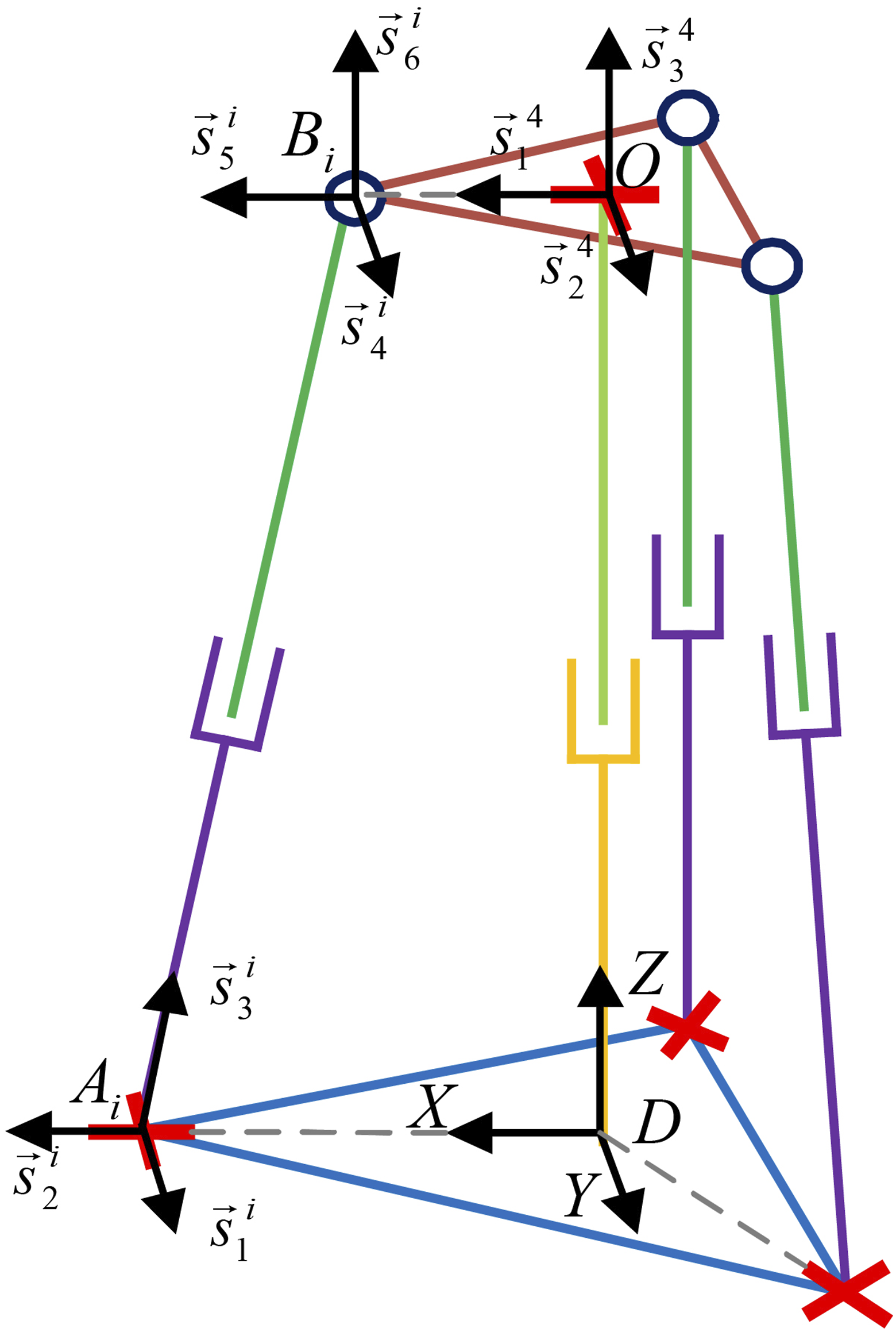

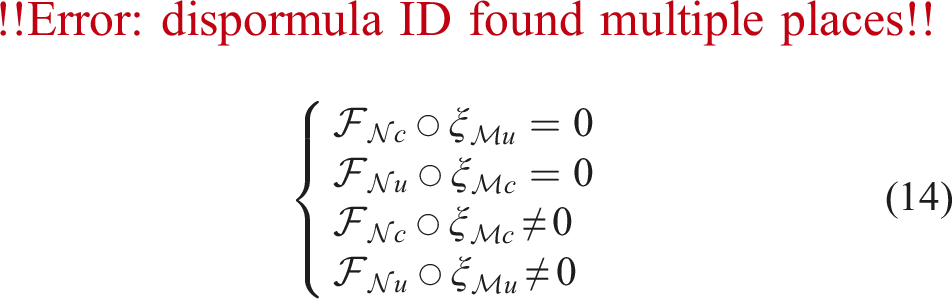
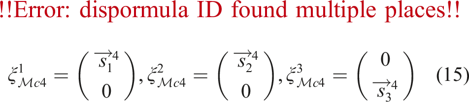
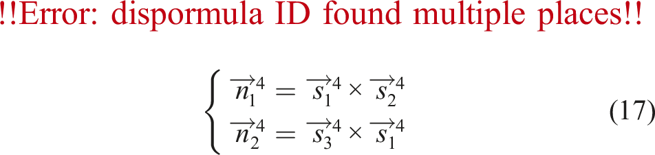
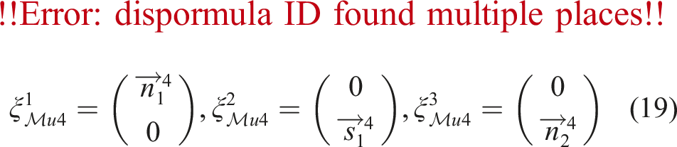
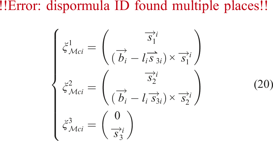
For the kinematic chain OD, its four subspace screw’s bases can be written according to the direct observation method (Tsai, 1999a), and the screw’s bases of its kinematic variational screw subspace are:

ξ_{M c 4}^{1} = (\begin{matrix} {\vec{s}}_{1}^{4} \\ 0 \end{matrix}), ξ_{M c 4}^{2} = (\begin{matrix} {\vec{s}}_{2}^{4} \\ 0 \end{matrix}), ξ_{M c 4}^{3} = (\begin{matrix} 0 \\ {\vec{s}}_{3}^{4} \end{matrix})

(15)

The screw’s base of the constraining wrench subspace is:

F_{N u 4}^{1} = (\begin{matrix} {\vec{n}}_{1}^{4} \\ 0 \end{matrix}), F_{N u 4}^{2} = (\begin{matrix} 0 \\ {\vec{s}}_{1}^{4} \end{matrix}), F_{N u 4}^{3} = (\begin{matrix} 0 \\ {\vec{n}}_{2}^{4} \end{matrix})

(16)

where,

\{\begin{cases} {\vec{n}}_{1}^{4} = {\vec{s}}_{1}^{4} \times {\vec{s}}_{2}^{4} \\ {\vec{n}}_{2}^{4} = {\vec{s}}_{3}^{4} \times {\vec{s}}_{1}^{4} \end{cases}

(17)

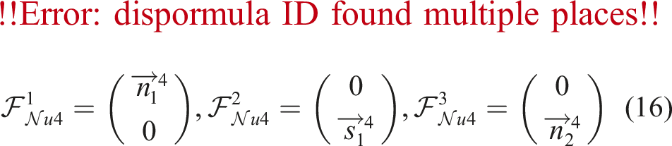
According to the dual relation and the kinematic variational screw subspace, we can get the bases of the actuation wrench subspace:

F_{N c 4}^{1} = (\begin{matrix} {\vec{s}}_{1}^{4} \\ 0 \end{matrix}), F_{N u 4}^{2} = (\begin{matrix} {\vec{s}}_{2}^{4} \\ 0 \end{matrix}), F_{N u 4}^{3} = (\begin{matrix} 0 \\ {\vec{s}}_{3}^{4} \end{matrix})

(18)

Similarly, we can get the bases of the constraining variational screw subspace:

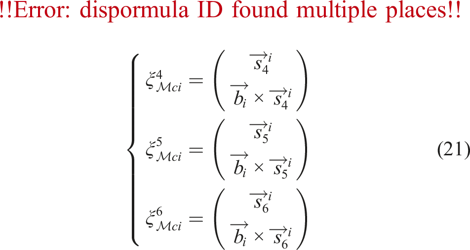
ξ_{M u 4}^{1} = (\begin{matrix} {\vec{n}}_{1}^{4} \\ 0 \end{matrix}), ξ_{M u 4}^{2} = (\begin{matrix} 0 \\ {\vec{s}}_{1}^{4} \end{matrix}), ξ_{M u 4}^{3} = (\begin{matrix} 0 \\ {\vec{n}}_{2}^{4} \end{matrix})

(19)

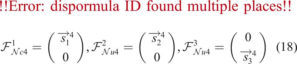
The kinematic chain A_iB_i is an unconstrained branched chain with six independent screw’s bases, and the screw’s bases in the kinematic variational screw subspace can be written out by the direct observation method:

\{\begin{cases} ξ_{M c i}^{1} = (\begin{matrix} {\vec{s}}_{1}^{i} \\ ({\vec{b}}_{i} - l_{i} {\overset{⇀}{s}}_{3 i}) \times {\vec{s}}_{1}^{i} \end{matrix}) \\ ξ_{M c i}^{2} = (\begin{matrix} {\vec{s}}_{2}^{i} \\ ({\vec{b}}_{i} - l_{i} {\vec{s}}_{3 i}) \times {\vec{s}}_{2}^{i} \end{matrix}) \\ ξ_{M c i}^{3} = (\begin{matrix} 0 \\ {\vec{s}}_{3}^{i} \end{matrix}) \end{cases}

(20)

\{\begin{cases} ξ_{M c i}^{4} = (\begin{matrix} {\vec{s}}_{4}^{i} \\ {\vec{b}}_{i} \times {\vec{s}}_{4}^{i} \end{matrix}) \\ ξ_{M c i}^{5} = (\begin{matrix} {\vec{s}}_{5}^{i} \\ {\vec{b}}_{i} \times {\vec{s}}_{5}^{i} \end{matrix}) \\ ξ_{M c i}^{6} = (\begin{matrix} {\vec{s}}_{6}^{i} \\ {\vec{b}}_{i} \times {\vec{s}}_{6}^{i} \end{matrix}) \end{cases}

(21)

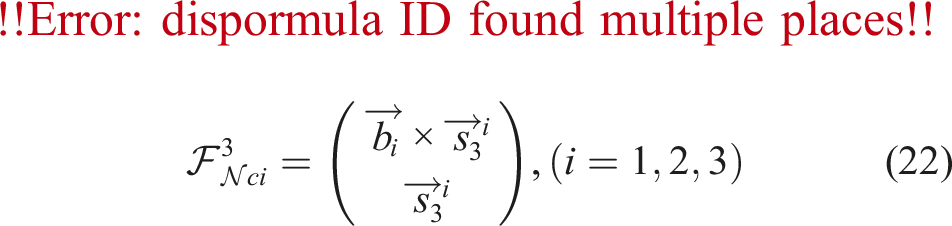
The drive on A_iB_i has only moving joints, so its actuation wrench subspace has only one nonzero screw:

F_{N c i}^{3} = (\begin{matrix} {\vec{b}}_{i} \times {\vec{s}}_{3}^{i} \\ {\vec{s}}_{3}^{i} \end{matrix}), (i = 1,2,3)

(22)

According to the principle of mechanism composition, the velocity of the end-effector platform of a parallel robot is constituted by the intersection of all the end points of its motion chains, for the relationship between the kinematic chain A_iB_i and the moving platform, we can get:

ξ_{M} = \sum_{j = 1}^{6} δ ρ_{c i}^{j} ξ_{M c i}^{j}, (i = 1,2,3)

(23)

where

ξ_{M}

is the moving platform variational screw;

δ ρ_{c i}^{j}

is the variational on the helical base

ξ_{M c i}^{j}

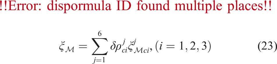
There is a relationship between the kinematic chain OD and the mobile platform:

ξ_{M} = \sum_{j c = 1}^{3} δ ρ_{c 4}^{j c} ξ_{M c 4}^{j c} + \sum_{j u = 1}^{3} δ ρ_{u 4}^{j u} ξ_{M u 4}^{j u}

(24)

where

δ ρ_{c 4}^{j c}

is the variate on the screw’s base

ξ_{M c 4}^{j c}

;

δ ρ_{u 4}^{j u}

is the variate on the helical base

ξ_{M u 4}^{j u}

Reciprocal product operations are performed on both sides of equation (23) for the driving wrench $F_{N c}$ :

F_{N c} ○ ξ_{M} = F_{N c} ○ \sum_{j = 1}^{6} δ ρ_{c i}^{j} ξ_{M c i}^{j}, (i = 1,2,3)

(25)

Since the 3UPU/PS parallel robots are driven only by moving subs on A_iB_i, that is, the actuation wrench subspace $N_{c}$ has only the element $F_{N c i}^{3}$ , it is:

{(F_{N c i}^{3})}^{T} ξ_{M} = {(F_{N c i}^{3})}^{T} ξ_{M c i}^{3} δ ρ_{c i}^{3}, (i = 1,2,3)

(26)

Taking reciprocal product operation for both sides of equation (24) with respect to $F_{N u 4}^{k}$ , due to the orthogonal relationship between the constraining wrench subspace and the kinematic variational screw subspace, we can obtain:

{(F_{N u 4}^{k})}^{T} ξ_{M} = {(F_{N u 4}^{k})}^{T} ξ_{M u 4}^{k} δ ρ_{u 4}^{k}, (k = 1,2,3)

(27)

Equations (26) and (27) constitute the generalized velocity Jacobian matrix of the 3UPS/PU parallel robot:

J_{L} ξ_{M} = J_{R} δ ρ

(28)

where:

\{\begin{cases} J_{L} = [\begin{matrix} {({\vec{b}}_{1} \times {\vec{s}}_{3}^{1})}^{T} & {({\vec{s}}_{3}^{1})}^{T} \\ {({\vec{b}}_{2} \times {\vec{s}}_{3}^{2})}^{T} & {({\vec{s}}_{3}^{2})}^{T} \\ {({\vec{b}}_{3} \times {\vec{s}}_{3}^{3})}^{T} & {({\vec{s}}_{3}^{3})}^{T} \\ {({\vec{n}}_{1}^{4})}^{T} & 0 \\ 0 & {({\vec{s}}_{1}^{4})}^{T} \\ 0 & {({\vec{n}}_{2}^{4})}^{T} \end{matrix}] \\ J_{R} = [\begin{matrix} I_{3 \times 3} & 0 \\ 0 & I_{3 \times 3} \end{matrix}] \\ ξ_{M} = [\begin{matrix} δ α \\ δ β \\ δ γ \\ δ x \\ δ y \\ δ z \end{matrix}], δ ρ = [\begin{matrix} δ ρ_{c 1}^{3} \\ δ ρ_{c 2}^{3} \\ δ ρ_{c 3}^{3} \\ δ ρ_{u 4}^{1} \\ δ ρ_{u 4}^{2} \\ δ ρ_{u 4}^{3} \end{matrix}] \end{cases}

(29)

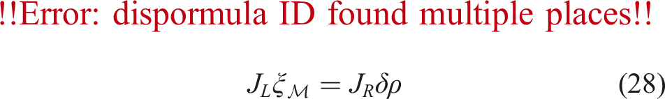
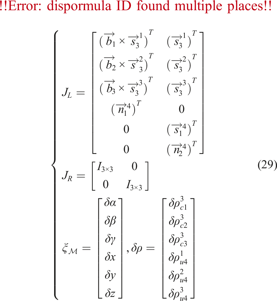
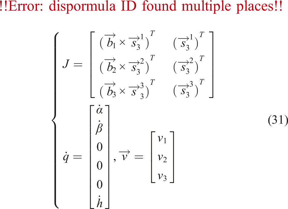
The initial three rows of the generalized velocity Jacobian matrix describe the connection between the parallel robot’s platform velocity and the drive velocity. This relationship can be expressed as:

J \dot{q} = v

(30)

where:

\{\begin{cases} J = [\begin{matrix} \begin{matrix} {({\vec{b}}_{1} \times {\vec{s}}_{3}^{1})}^{T} \\ {({\vec{b}}_{2} \times {\vec{s}}_{3}^{2})}^{T} \\ {({\vec{b}}_{3} \times {\vec{s}}_{3}^{3})}^{T} \end{matrix} & \begin{matrix} {({\vec{s}}_{3}^{1})}^{T} \\ {({\vec{s}}_{3}^{2})}^{T} \\ {({\vec{s}}_{3}^{3})}^{T} \end{matrix} \end{matrix}] \\ \dot{q} = [\begin{matrix} \dot{α} \\ \dot{β} \\ 0 \\ 0 \\ 0 \\ \dot{h} \end{matrix}], \vec{v} = [\begin{matrix} v_{1} \\ v_{2} \\ v_{3} \end{matrix}] \end{cases}

(31)

where

{\vec{v}}_{i}

is the velocity of the moving joint on chain A_iB_i.

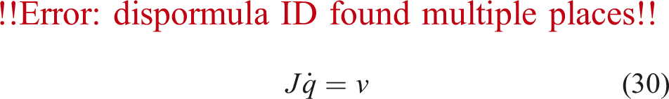
Taking the time derivative of equation (30), we obtain the connection between platform acceleration and drive acceleration:

\vec{a} = \dot{J} \dot{q} + J \ddot{q}

(32)

\{\begin{cases} \dot{J} = [\begin{matrix} \begin{matrix} {(\vec{ω} \times {\vec{b}}_{1} \times {\vec{s}}_{3}^{1} + {\vec{b}}_{1} \times ({\vec{ω}}_{1} \times {\vec{s}}_{3}^{1}))}^{T} \\ {(\vec{ω} \times {\vec{b}}_{2} \times {\vec{s}}_{3}^{2} + {\vec{b}}_{2} \times ({\vec{ω}}_{2} \times {\vec{s}}_{3}^{2}))}^{T} \\ {(\vec{ω} \times {\vec{b}}_{3} \times {\vec{s}}_{3}^{3} + {\vec{b}}_{3} \times ({\vec{ω}}_{3} \times {\vec{s}}_{3}^{3}))}^{T} \end{matrix} & \begin{matrix} {({\vec{ω}}_{1} \times {\vec{s}}_{3}^{1})}^{T} \\ {({\vec{ω}}_{2} \times {\vec{s}}_{3}^{2})}^{T} \\ {({\vec{ω}}_{3} \times {\vec{s}}_{3}^{3})}^{T} \end{matrix} \end{matrix}] \\ \ddot{q} = [\begin{matrix} \ddot{α} & \ddot{β} & 0 & 0 & 0 & \ddot{h} \end{matrix}] \end{cases}

(33)

where

\vec{a}

represents the acceleration of the moving joint,

\ddot{q}

represents the acceleration screw of the moving platform,

{\vec{ω}}_{i}

represents the angular velocity of A_iB_i’s rotation, and

\vec{ω}

represents the angular velocity of the rotation of the parallel robotic motion platform.

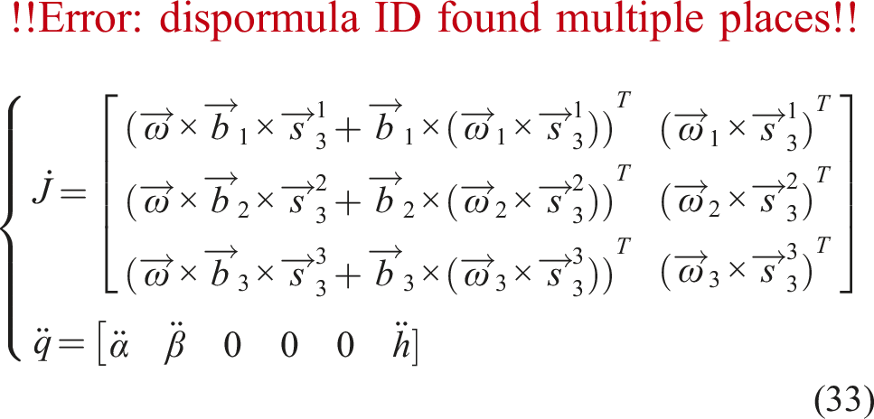
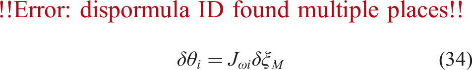
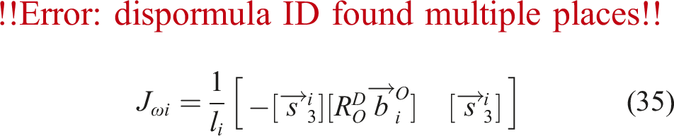
From equation (9), we obtain the Jacobian matrix J_ωi, which relates the variation in the angle of A_iB_i to the variation in the moving platform’s screw:

δ θ_{i} = J_{ω i} δ ξ_{M}

(34)

J_{ω i} = \frac{1}{l_{i}} [\begin{matrix} - [{\vec{s}}_{3}^{i}] [R_{O}^{D} {\vec{b}}_{i}^{O}] & [{\vec{s}}_{3}^{i}] \end{matrix}]

(35)

From equation (13), we can get:

δ L_{ci1} = J_{ci1} δ ξ_{M}

(36)

J_{ci1} = \frac{l_{ci1}}{l_{i}} [\begin{matrix} {[{\vec{s}}_{3}^{i}]}^{2} [{\vec{b}}_{i}^{D}] & - {[{\vec{s}}_{3}^{i}]}^{2} \end{matrix}]

(37)

δ L_{ci2} = J_{ci2} δ ξ_{M}

(38)

J_{ci2} = \{[- [{\vec{b}}_{i}^{D}], I_{3 \times 3}] + l_{i} [{\vec{s}}_{3}^{i}] J_{ω i} + (l_{ci2} - l_{i}) [{\vec{s}}_{3}^{i}] J_{ω i}\}

(39)

where J_ci1 is the Jacobi matrix describing the relationship between the center-of-mass variation of the lower linkage of A_iB_i and the moving platform variational screw;J_ci2 is the Jacobi matrix describing the relationship between the center-of-mass variant of the upper linkage of A_iB_i and the moving platform variational screw.

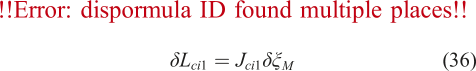
The Jacobi matrix describing the relationship between the variational screw of the lower linkage center of mass of A_iB_i and the variational screw of the moving platform is:

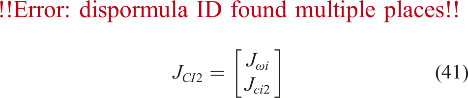
J_{CI1} = [\begin{matrix} J_{ω i} \\ J_{ci1} \end{matrix}]

(40)

The Jacobi matrix describing the relationship between the variational screw of the center of mass of the upper link of A_iB_i and the variational screw of the moving platform is:

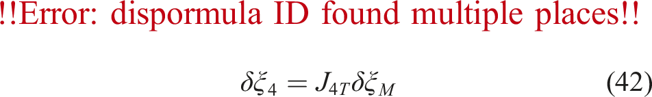
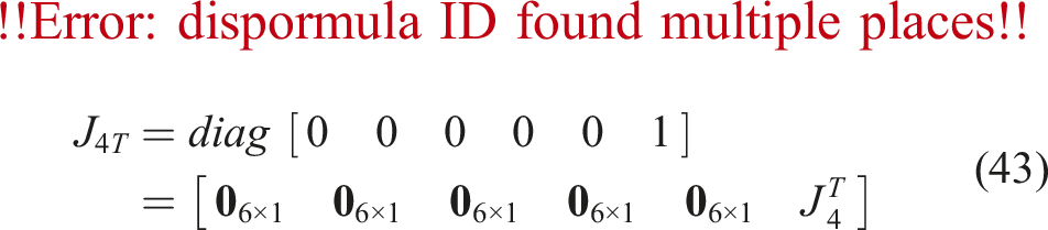
J_{CI2} = [\begin{matrix} J_{ω i} \\ J_{ci2} \end{matrix}]

(41)

For the chain OD, whose center-of-mass velocity is the same as that of the moving platform and which has only translational displacement, in order to uniformly translate the motion variability to the variational screw of the moving platform, the Jacobi matrix between the variational screw δξ₄ of the center-of-mass of the chain OD and the variational screw of the moving platform is expressed as:

δ ξ_{4} = J_{4 T} δ ξ_{M}

(42)

where:

\begin{aligned} J_{4 T} & = d i a g [\begin{matrix} 0 & 0 & 0 & 0 & 0 & 1 \end{matrix}] \\ = [\begin{matrix} 0_{6 \times 1} & 0_{6 \times 1} & 0_{6 \times 1} & 0_{6 \times 1} & 0_{6 \times 1} & J_{4}^{T} \end{matrix}] \end{aligned}

(43)

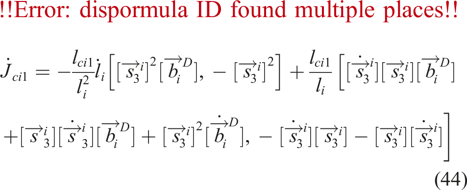
For logical clarity, here we directly present the results after taking the first-order derivative of the Jacobian matrices (35), (37), and (39) with respect to time:

\begin{matrix} {\dot{J}}_{ci1} = - \frac{l_{ci1}}{l_{i}^{2}} {\dot{l}}_{i} [{[{\vec{s}}_{3}^{i}]}^{2} [{\vec{b}}_{i}^{D}], - {[{\vec{s}}_{3}^{i}]}^{2}] + \frac{l_{ci1}}{l_{i}} [[{\dot{\vec{s}}}_{3}^{i}] [{\vec{s}}_{3}^{i}] [{\vec{b}}_{i}^{D}] \\ + [{\vec{s}}_{3}^{i}] [{\dot{\vec{s}}}_{3}^{i}] [{\vec{b}}_{i}^{D}] + {[{\vec{s}}_{3}^{i}]}^{2} [{\dot{\vec{b}}}_{i}^{D}], - [{\dot{\vec{s}}}_{3}^{i}] [{\vec{s}}_{3}^{i}] - [{\vec{s}}_{3}^{i}] [{\dot{\vec{s}}}_{3}^{i}]] \end{matrix}

(44)

\begin{matrix} {\dot{J}}_{ci2} = [- [{\vec{b}}_{i}^{D}], O_{3 \times 3}] + {\dot{l}}_{i} [{\vec{s}}_{3}^{i}] J_{ω i} + l_{i} [{\dot{\vec{s}}}_{3}^{i}] J_{ω i} + l_{i} [{\vec{s}}_{3}^{i}] {\dot{J}}_{ω i} \\ - {\dot{l}}_{i} [{\vec{s}}_{3}^{i}] J_{ω i} + (l_{ci2} - l_{i}) [{\dot{\vec{s}}}_{3}^{i}] J_{ω i} + (l_{ci2} - l_{i}) [{\vec{s}}_{3}^{i}] {\dot{J}}_{ω i} \end{matrix}

(45)

\begin{matrix} {\dot{J}}_{ω i} = - \frac{1}{l_{i}^{2}} {\dot{l}}_{i} [- [{\vec{s}}_{3}^{i}] [{\vec{b}}_{i}^{D}], [{\vec{s}}_{3}^{i}]] \\ + \frac{1}{l_{i}} [- [{\dot{\vec{s}}}_{3}^{i}] [{\vec{b}}_{i}^{D}] - [{\vec{s}}_{3}^{i}] [{\dot{\vec{b}}}_{i}^{D}], [{\dot{\vec{s}}}_{3}^{i}]] \end{matrix}

(46)

3. Dynamic model construction based on screw theory and d’Alembert-Lagrange equation

This paper aims to model the dynamics of parallel robots accurately. Without the need for intermediate joint force variables, we focus on the control problem. Employing the screw-based d’Alembert-Lagrange equation approach, we construct a control model specifically designed for parallel robots.

The d’Alembert-Lagrange equations, also known as the virtual work principle of dynamics, represent a powerful analytical tool in mechanics. These equations combine d’Alembert’s principle with the virtual displacement principle. Unlike Newton’s Euler equations, which necessitate calculating constraint forces for each joint, the d’Alembert-Lagrange equations simplify the dynamics analysis of parallel robots by eliminating the need to compute intermediate forces. This advantage is particularly pronounced for complex dynamic systems like parallel robots with numerous coupled joints. In the context of parallel robots, where non-driven joints do not contribute to the force dynamics, the d’Alembert-Lagrange equations are more suitable. Moreover, they facilitate obtaining explicit analytical solutions—an advantage over the Lagrange equations, which involve extensive derivative operations.

The screw theory, based on Lie group and Lie algebra, offers a more suitable tool for representing spatial motion, particularly for expressing the spatial force and velocity of a rigid body. Moreover, it simplifies the calculation of the inertial wrench in rigid body space, as shown in equation (47), thereby facilitating the integration of screw theory with the d’Alembert-Lagrange equations. This integration is based on the principle of energy conservation, similar to bonding diagrams (Guo et al., 2015; Ma et al., 2018), and incorporates external force, inertial force, and virtual displacement as main elements. The concept of energy can be extended from virtual work, an energy mediator, to the operation of screw quantities. Utilizing the screw form for the three main elements in the d’Alembert-Lagrange equation—external force, inertial force, and virtual displacement—allows the virtual displacement to correspond to the element of the variational screw in the movable variational space. Meanwhile, the force vector can be generalized to the wrench, and the computation of inertial force can be replaced by that of the inertial wrench.

Let the external force on the moving platform be ${\vec{F}}_{O}$ , the external moment be ${\vec{M}}_{O}$ , and the gravitational force on the moving platform is ${\vec{G}}_{O}$ , then the external wrench $F_{O 1}^{D}$ on the moving platform is:

F_{O 1}^{D} = [\begin{matrix} {\vec{M}}_{O} \\ {\vec{F}}_{O} + {\vec{G}}_{O} \end{matrix}]

(47)

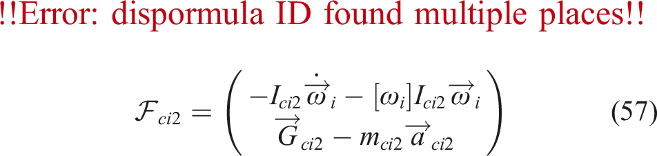
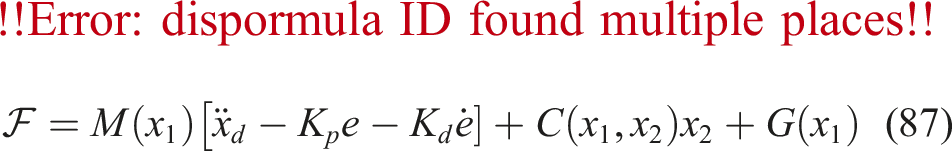
From the equation for the inertial wrench rotation of a rigid body (see Appendix for detailed derivation), the inertial wrench $F_{O 2}$ received by the moving platform in space can be calculated as:

F_{O 2}^{D} = - G_{O}^{D} \dot{V} + [a d_{V}] G_{O}^{D} V

(48)

where

V

is the velocity screw of the moving platform in the base coordinate system

\{D\}

G_{O}^{D}

is the spatial inertia matrix of the moving platform in the base coordinate system

\{D\}

, and [ad_V]is the Li bracket’s concomitant operator, Lynch and Park (2017) derive the transformation from the spatial inertia matrix in the center-of-mass coordinate system to the spatial inertia matrix in the base coordinate system from kinetic-energy equivalence relations (Tsai, 1999a):

G_{O}^{D} = {[A d_{T_{O D}}]}^{T} G_{O}^{O} [A d_{T_{O D}}], G_{O}^{D} \in R^{6 \times 6}

(49)

[A d_{T_{O D}}] = [\begin{matrix} R & 0 \\ [p] R & R \end{matrix}]

(50)

where

[A d_{T_{O D}}]

is the concomitant operator of the Lie group for the transformation of the screw from the coordinate system

\{D\}

to the coordinate system

\{O\}

The virtual work of moving the platform for:

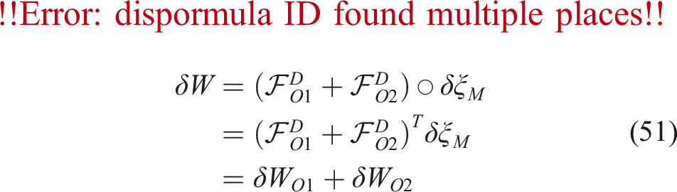
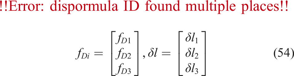
\begin{aligned} δ W & = (F_{O 1}^{D} + F_{O 2}^{D}) ○ δ ξ_{M} \\ = {(F_{O 1}^{D} + F_{O 2}^{D})}^{T} δ ξ_{M} \\ = δ W_{O 1} + δ W_{O 2} \end{aligned}

(51)

The virtual work done by the driving force ${\vec{F}}_{b i}$ on the chain A_iB_i is:

{\vec{F}}_{b i} \cdot δ {\vec{l}}_{i} = f_{D i} {[\begin{matrix} 0 \\ {\vec{s}}_{3}^{i} \end{matrix}]}^{T} \cdot [\begin{matrix} 0 \\ {\vec{s}}_{3}^{i} \end{matrix}] δ l_{i} = f_{D i} δ l_{i}

(52)

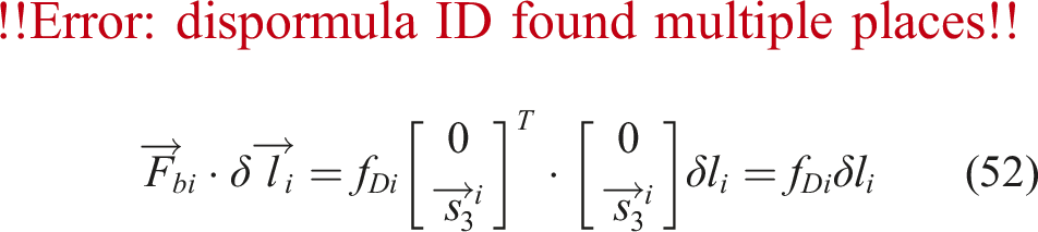
The virtual work done by the driving force on all chains $A_{i} B_{i} (i = 1,2,3)$ is:

δ W_{D} = f_{D i} ○ δ l = f_{D i}^{T} δ l = f_{D i}^{T} J δ ξ_{M}

(53)

f_{D i} = [\begin{matrix} f_{D 1} \\ f_{D 2} \\ f_{D 3} \end{matrix}], δ l = [\begin{matrix} δ l_{1} \\ δ l_{2} \\ δ l_{3} \end{matrix}]

(54)

where f_Di is the force generated by the ith actuator, and δl_i is the displacement variation of the actuator.

Suppose that a robot has two variational screws δξ₁ and δξ₂, and the relationship between the two variational screws is δξ₂ = J₂₁δξ₁, so the work of the wrench $F_{2}$ corresponding to the variational screw δξ₂ is as follows:

\begin{aligned} δ W_{12} & = F_{2} ○ δ ξ_{2} \\ = F_{2}^{T} δ ξ_{2} \\ = F_{2}^{T} J_{21} δ ξ_{1} \\ = {(F_{2}^{1})}^{T} δ ξ_{1} \end{aligned}

(55)

F_{2}^{1} = J^{T} F_{2}

(56)

where

F_{2}^{1}

is the generalized wrench of the wrench

F_{2}

in the direction of δξ₁. The gravity of the upper rod of the A_iB_i chain is

{\vec{G}}_{ci2}

, and the wrench generated by the gravity and inertial force of the upper rod at the center of mass of the upper rod of the A_iB_i chain is:

F_{ci2} = (\begin{matrix} - I_{ci2} {\dot{\vec{ω}}}_{i} - [ω_{i}] I_{ci2} {\vec{ω}}_{i} \\ {\vec{G}}_{ci2} - m_{ci2} {\vec{a}}_{ci2} \end{matrix})

(57)

where, I_ci2, m_ci2 and

{\vec{a}}_{ci2}

are the moment of inertia, mass and acceleration at the center of mass of the upper connecting rod of A_iB_i.

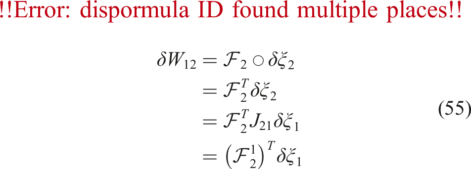
It can be seen from equation (56) that the generalized wrench generated by the wrench $F_{ci2}$ in the δξ direction is:

F_{ci2}^{O} = J_{CI2}^{T} F_{ci2}

(58)

The virtual work generated by the upper rod of the A_iB_i chain is:

δ W_{ci2} = F_{ci2}^{O} ○ δ ξ_{M} = {(F_{ci2}^{O})}^{T} δ ξ_{M}

(59)

The gravity of the lower connecting rod of the A_iB_i chain is ${\vec{G}}_{ci1}$ , and the wrench generated by the gravity and inertial force of the lower connecting rod at the center of mass of the lower rod of the chain A_iB_i is:

F_{ci1} = (\begin{matrix} - I_{ci1} {\dot{\vec{ω}}}_{i} - [{\vec{ω}}_{i}] I_{ci1} {\vec{ω}}_{i} \\ {\vec{G}}_{ci1} - m_{ci1} {\vec{a}}_{ci1} \end{matrix})

(60)

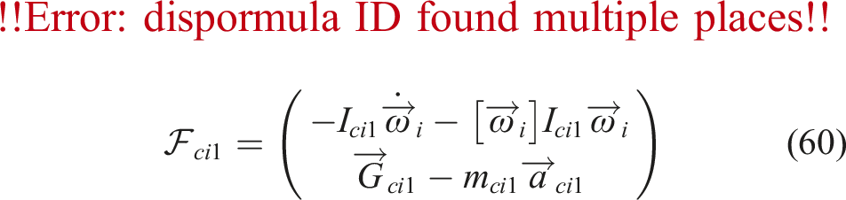
The generalized wrench generated by the wrench $F_{ci1}$ in the δξ direction is:

F_{ci1}^{O} = J_{CI1}^{T} F_{ci1}

(61)

The virtual work generated by the lower rod of A_iB_i chain is:

δ W_{ci1} = F_{ci1}^{O} ○ δ ξ_{M} = {(F_{ci1}^{O})}^{T} δ ξ_{M}

(62)

The virtual work generated by the kinematic chain A_iB_i is:

δ W_{c i} = δ W_{ci1} + δ W_{ci2}

(63)

Let the mass of the movable part of the chain OD be m₄, then the inertia wrench of the centroid position of the chain OD is:

F_{4} = {[\begin{matrix} 0 & 0 & 0 & 0 & 0 & - m_{4} g \end{matrix}]}^{T}

(64)

We can conclude that the virtual work generated by the inertia wrench $F_{4}^{O}$ on the chain OD is:

δ W_{4} = (F_{O}^{4}) ○ δ ξ_{M} = {(F_{O}^{4})}^{T} δ ξ_{M}

(65)

where

F_{O}^{4} = J_{4 T}^{T} F_{4}

(66)

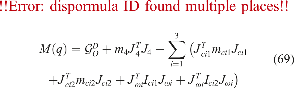
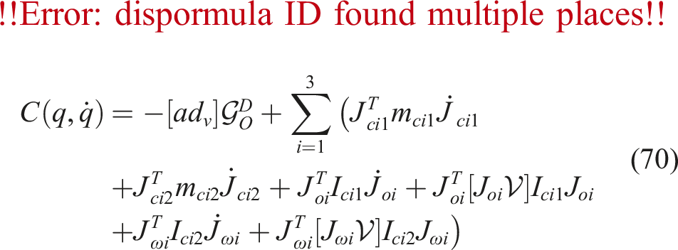
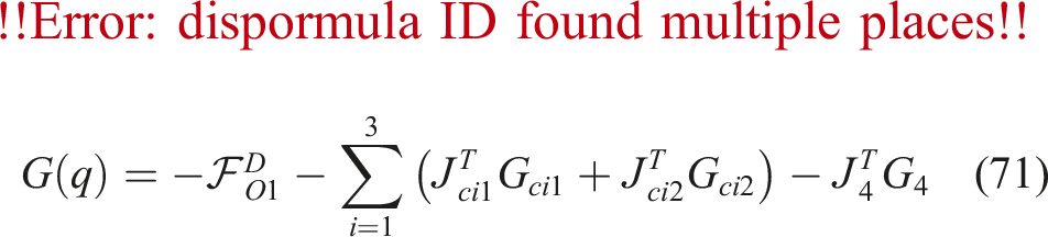
According to the d’Alembert-Lagrange equation, the dynamic equation of the parallel robot can be obtained by adding the virtual work generated by the above inertial wrench and the external wrench:

δ W_{O} + δ W_{D} + \sum_{i = 1}^{3} δ W_{c i} + δ W_{4} = 0

(67)

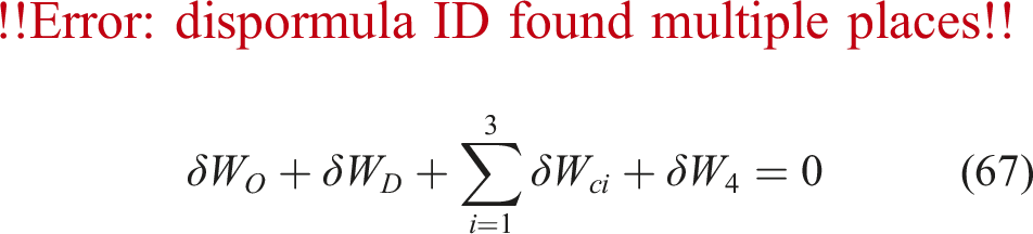
The rotation matrix and all the shape and position parameters of the parallel robot are brought in. Since δξ_M ≠ 0, equation (67) can eliminate δξ_M and simplify it, and obtain:

F = M (q) \ddot{q} + C (q, \dot{q}) \dot{q} + G (q)

(68)

\begin{matrix} M (q) = G_{O}^{D} + m_{4} J_{4}^{T} J_{4} + \sum_{i = 1}^{3} (J_{ci1}^{T} m_{ci1} J_{ci1} \\ + J_{ci2}^{T} m_{ci2} J_{ci2} + J_{ω i}^{T} I_{ci1} J_{ω i} + J_{ω i}^{T} I_{ci2} J_{ω i}) \end{matrix}

(69)

\begin{aligned} C (q, \dot{q}) & = - [a d_{ν}] G_{O}^{D} + \sum_{i = 1}^{3} (J_{ci1}^{T} m_{ci1} {\dot{J}}_{ci1} \\ + J_{ci2}^{T} m_{ci2} {\dot{J}}_{ci2} + J_{o i}^{T} I_{ci1} {\dot{J}}_{o i} + J_{o i}^{T} [J_{o i} V] I_{ci1} J_{o i} \\ + J_{ω i}^{T} I_{ci2} {\dot{J}}_{ω i} + J_{ω i}^{T} [J_{ω i} V] I_{ci2} J_{ω i}) \end{aligned}

(70)

G (q) = - F_{O 1}^{D} - \sum_{i = 1}^{3} (J_{ci1}^{T} G_{ci1} + J_{ci2}^{T} G_{ci2}) - J_{4}^{T} G_{4}

(71)

where,

q \in R^{6 \times 1}

is the displacement of the moving platform at the end of the parallel robot.

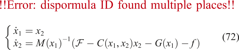
4. Controller design

In this paper, we further discuss the control problem of parallel robots using the explicit robot dynamics equation (equation (68)). In the pseudo-linear dynamic model of the parallel robot, dynamic parameters change with the posture. Additionally, the modeling process does not consider the effects of unmodeled dynamics such as the frictions and other time-varying disturbances (Wu et al., 2021). These factors can lead to inaccuracies in the model. Therefore, we introduce unmodeled dynamics and external disturbances into the control model to improve the accuracy of the mathematical description of parallel robots, thereby providing a foundation for the design of high-precision controllers for parallel robots.

\{\begin{cases} {\dot{x}}_{1} = x_{2} \\ {\dot{x}}_{2} = M {(x_{1})}^{- 1} (F - C (x_{1}, x_{2}) x_{2} - G (x_{1}) - f) \end{cases}

(72)

where f = f(x₁, x₂, t) is the sum of unmodeled error and external disturbance force x₁ = q,

x_{2} = \dot{q}

;

4.1. Control strategy design

To address the difficulty of traditional control models in resisting uncertain interference and to improve the accuracy and robustness of robot control, we employ the sliding mode control method to design the robot’s control strategy, thereby reducing the dependence on an accurate robot model.

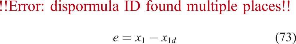
The robot’s error is defined as:

e = x_{1} - x_{1 d}

(73)

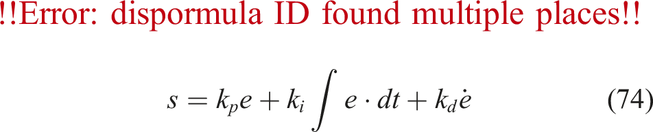
The integral sliding surface is defined as:

s = k_{p} e + k_{i} \int e \cdot d t + k_{d} \dot{e}

(74)

To eliminate the chattering problem in sliding mode control, a chattering-free hyperbolic convergence law (Tao et al., 2018) is used to design the controller. This reaching law ensures that the sliding variable remains far from the sliding surface when the surface’s speed is high, and decreases rapidly when the sliding variable is very close to the sliding surface. This feature allows the controller to quickly reach the sliding surface without chattering (Zhao et al., 2024a). The convergence rate is determined by hyperbolic sine and hyperbolic tangent functions:

\{\begin{cases} \dot{s} = - s_{1} - s_{2} \\ s_{1} = \frac{k_{1} - k_{1} e^{- 2 α s}}{1 + e^{- 2 α s}} = k_{1} \tanh (α s) \\ s_{2} = k_{2} |s| \cdot a s i n h (β s^{p}) \end{cases}

(75)

where k₁ > 0, k₂ > 0, α > 0, β > 0, γ > 0, p is positive odd number.

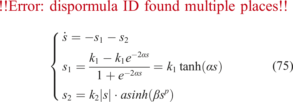
The impact of the parameters in equation (75) on the approaching speed of the sliding variable has been analyzed in detail in the article (Zhao et al., 2024b). The velocity of the sliding variable s near the sliding mold surface is controlled by adjusting k₁ and α, while k₂, β, and p determine the magnitude of s as it moves away from the surface. In this model, the parameters should not be too small to ensure sufficient approaching speed when the sliding variable s nears the sliding surface.

Deriving equation (74) to time, we can get:

\dot{s} = k_{p} \dot{e} + k_{i} e + k_{d} \ddot{e}

(76)

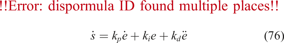
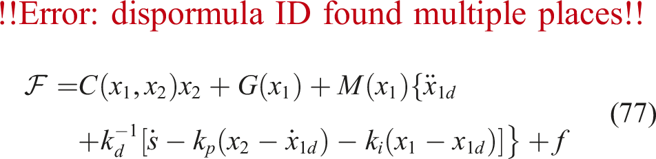
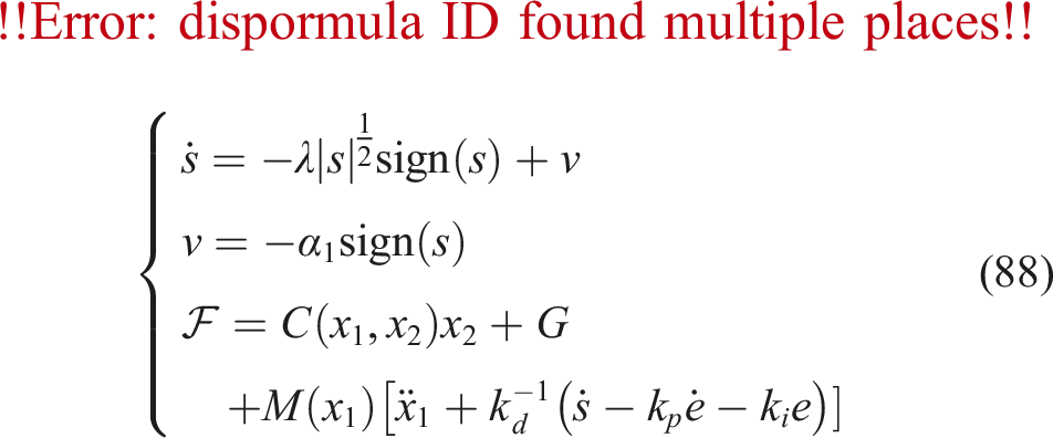
From equations (75) and (76), we can get the controller output should be:

\begin{matrix} \begin{matrix} F = C (x_{1}, x_{2}) x_{2} + G (x_{1}) + M (x_{1}) \{{\ddot{x}}_{1 d} \\ + k_{d}^{- 1} [\dot{s} - k_{p} (x_{2} - {\dot{x}}_{1 d}) - k_{i} (x_{1} - x_{1 d})]\} + f \end{matrix} \end{matrix}

(77)

4.2. Stability analysis

To prove the stability of the controller, the Lyapunov function is defined as:

V = \frac{1}{2} s \cdot s

(78)

The time derivative of the Lyapunov function is given by:

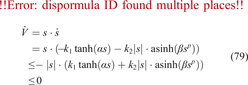
\begin{aligned} \dot{V} & = s \cdot \dot{s} \\ = s \cdot (- k_{1} \tanh (α s) - k_{2} |s| \cdot asinh (β s^{p})) \\ \leq - |s| \cdot (k_{1} \tanh (α s) + k_{2} |s| \cdot asinh (β s^{p})) \\ \leq 0 \end{aligned}

(79)

It can be observed from equation (79) that the designed controller satisfies the Lyapunov stability condition, ensuring that the system is asymptotically stable.

4.3. Hyperbolic convergence law sliding mode disturbance observer design

In traditional sliding mode control, to achieve zero steady-state error, the switching gain is usually set higher than the upper bound of the total disturbance and model uncertainty. However, this larger switching gain causes greater chattering. The hyperbolic convergence law sliding mode control can significantly reduce the system chattering caused by sliding mode switching. The purpose of designing this observer is to estimate the disturbance value, feed it back to the controller, and offset the disturbance at the controller level, thereby improving the system’s robustness.

Firstly, the disturbance part of the original system is defined as the extended state variable $z_{3} = - M {(x_{1})}^{- 1} f (x_{1}, x_{2}, t)$ , the derivative of z₃ is defined as ${\dot{z}}_{3} = w$ , z₁ and z₂ are used to represent the state variables x₁ and x₂ of the original system, respectively. Then the original system becomes:

\{\begin{cases} {\dot{z}}_{1} = z_{2} \\ {\dot{z}}_{2} = M {(z_{1})}^{- 1} [F - C (z_{1}, z_{2}) z_{2} - G (z_{1})] + z_{3} \\ {\dot{z}}_{3} = w \end{cases}

(80)

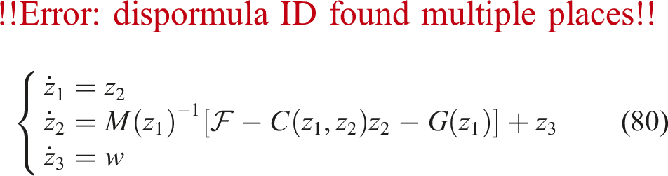
The observer is designed as:

\{\begin{cases} {\dot{\hat{z}}}_{1} = {\hat{z}}_{2} \\ {\dot{\hat{z}}}_{2} = M {(z_{1})}^{- 1} [F - C (z_{1}, z_{2}) z_{2} - G (z_{1})] + {\hat{z}}_{3} + μ_{g} \\ {\dot{\hat{z}}}_{3} = η μ_{g} \end{cases}

(81)

where μ_g is the input of the observer.

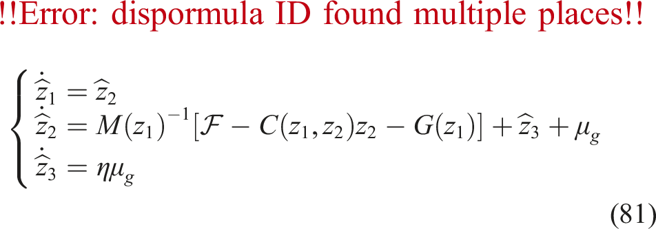
The observer error is defined as:

E_{i} = {\hat{z}}_{i} - z_{i} (i = 1,2,3)

(82)

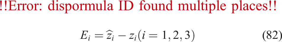
The error state equation obtained by subtracting equation (80) from equation (81) is:

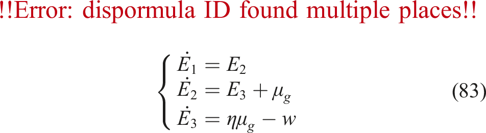
\{\begin{cases} {\dot{E}}_{1} = E_{2} \\ {\dot{E}}_{2} = E_{3} + μ_{g} \\ {\dot{E}}_{3} = η μ_{g} - w \end{cases}

(83)

The sliding mode surface of the observer is defined as S = E₂. The derivative of the sliding mode surface is $\dot{S} = {\dot{E}}_{2}$ . The input of the observer controller is designed as $μ_{g} = - k_{1} \cdot \tanh (α S) - k_{2} |S| \cdot a s i n h (β S^{p})$ . The Lyapunov function is defined as V₁ = 1/2S ⋅ S, and its time derivative is:

\begin{aligned} {\dot{V}}_{1} & = S \cdot \dot{S} \\ = S \cdot (E_{3} - k_{1} \cdot \tanh (α S) - k_{2} |S| \cdot asinh (β S^{p})) \\ \leq S \cdot E_{3} - k_{1} |\begin{matrix} S \end{matrix}| \cdot \tanh (\begin{matrix} α S \end{matrix}) - k_{2} |\begin{matrix} S \end{matrix}| \cdot |\begin{matrix} S \end{matrix}| \cdot asinh (\begin{matrix} β S^{p} \end{matrix}) \end{aligned}

(84)

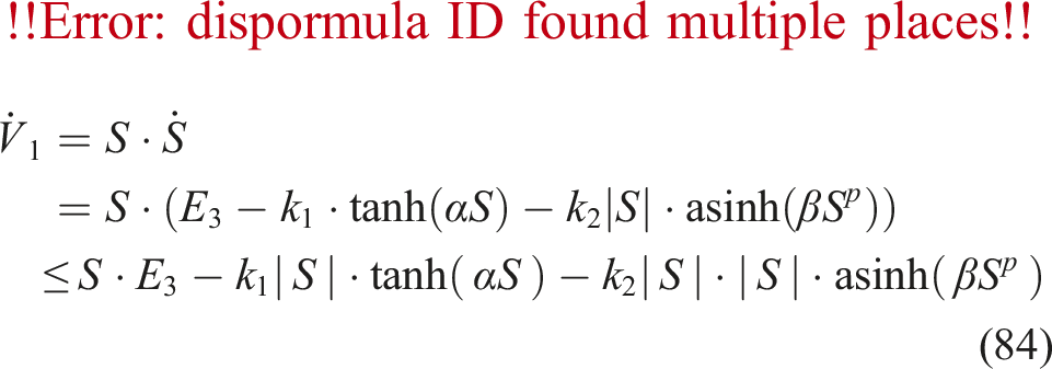
In equation (84), $- k_{2} |S| \cdot |S| \cdot asinh (β S^{p}) \leq 0$ . If $S \cdot E_{3} - k_{1} |S| \cdot \tanh (α S) \leq 0$ , that is, $\pm E_{3} \leq k_{1} \cdot \tanh (α S) \leq k_{1}$ , the observer can reach the sliding mode state in a finite time, we can get:

\{\begin{cases} E_{3} = - μ_{g} \\ {\dot{E}}_{3} = η μ_{g} - w \end{cases}

(85)

It can be solved by equation (85):

E_{3} = e^{- η t} C + e^{- η t} \int w (t) d t

(86)

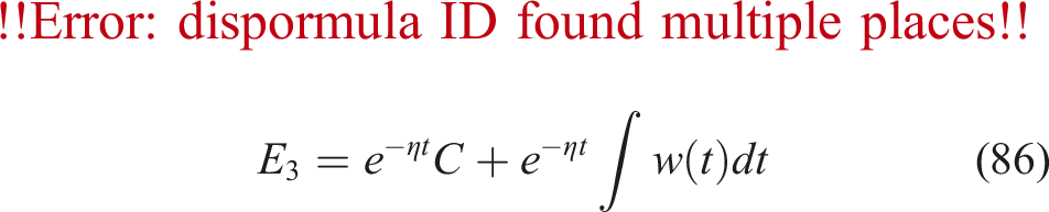
That is, the observation error of the observer to the disturbance can approach zero in a finite time.

The extended sliding mode observer based on the hyperbolic convergence law does not rely on an accurate mathematical model of the controlled object and does not require direct measurement of disturbances and their effects. This makes it particularly suitable for controlling parallel robots, which are challenging to model accurately (Gu et al., 2022). We combine the hyperbolic convergence law sliding mode controller with the observer to develop a control strategy for the parallel robot. The control scheme is illustrated in Figure 4.

Figure 4.

Schematic diagram of the control strategy.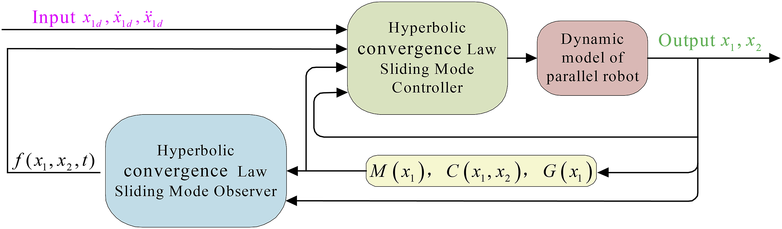

5. Simulation

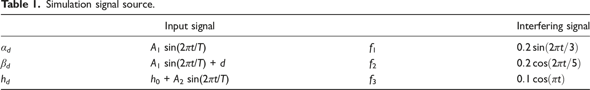
To verify the performance of the designed controller, we conducted simulations. The trajectory of the moving platform provided in the table was used as the simulation input, and an external interference signal was applied to the parallel robot (see Table 1). The tracking and error curves of the robot system are shown in Figures 5 and 6. As seen in Figure 6, the error in the three degrees of freedom of the parallel robot is controlled to the order of 10⁻⁵, indicating high control accuracy.

Table 1.

Simulation signal source.

	Input signal		Interfering signal
α _d	A₁ sin(2πt/T)	f ₁	$0.2 \sin (2 π t / 3)$
β _d	A₁ sin(2πt/T) + d	f ₂	$0.2 \cos (2 π t / 5)$
h _d	h₀ + A₂ sin(2πt/T)	f ₃	$0.1 \cos (π t)$

Figure 5.

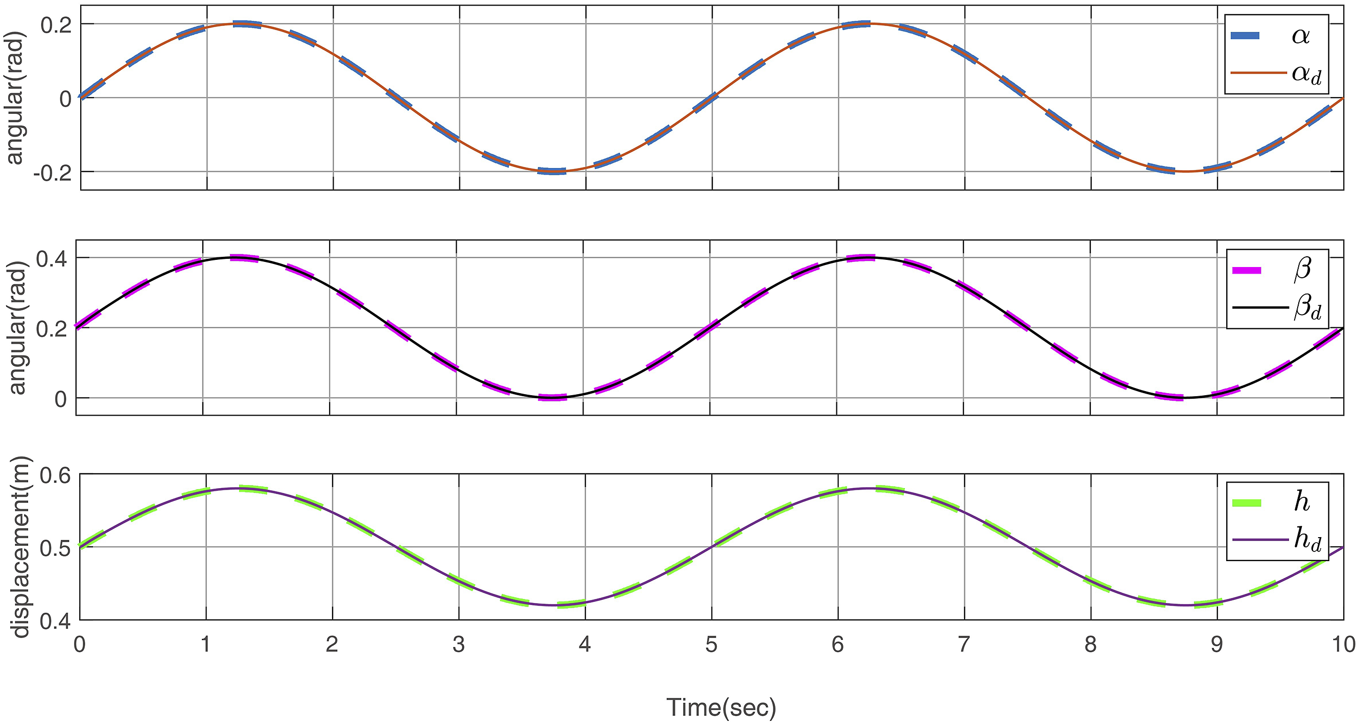
Trajectory tracking curve.

Figure 6.

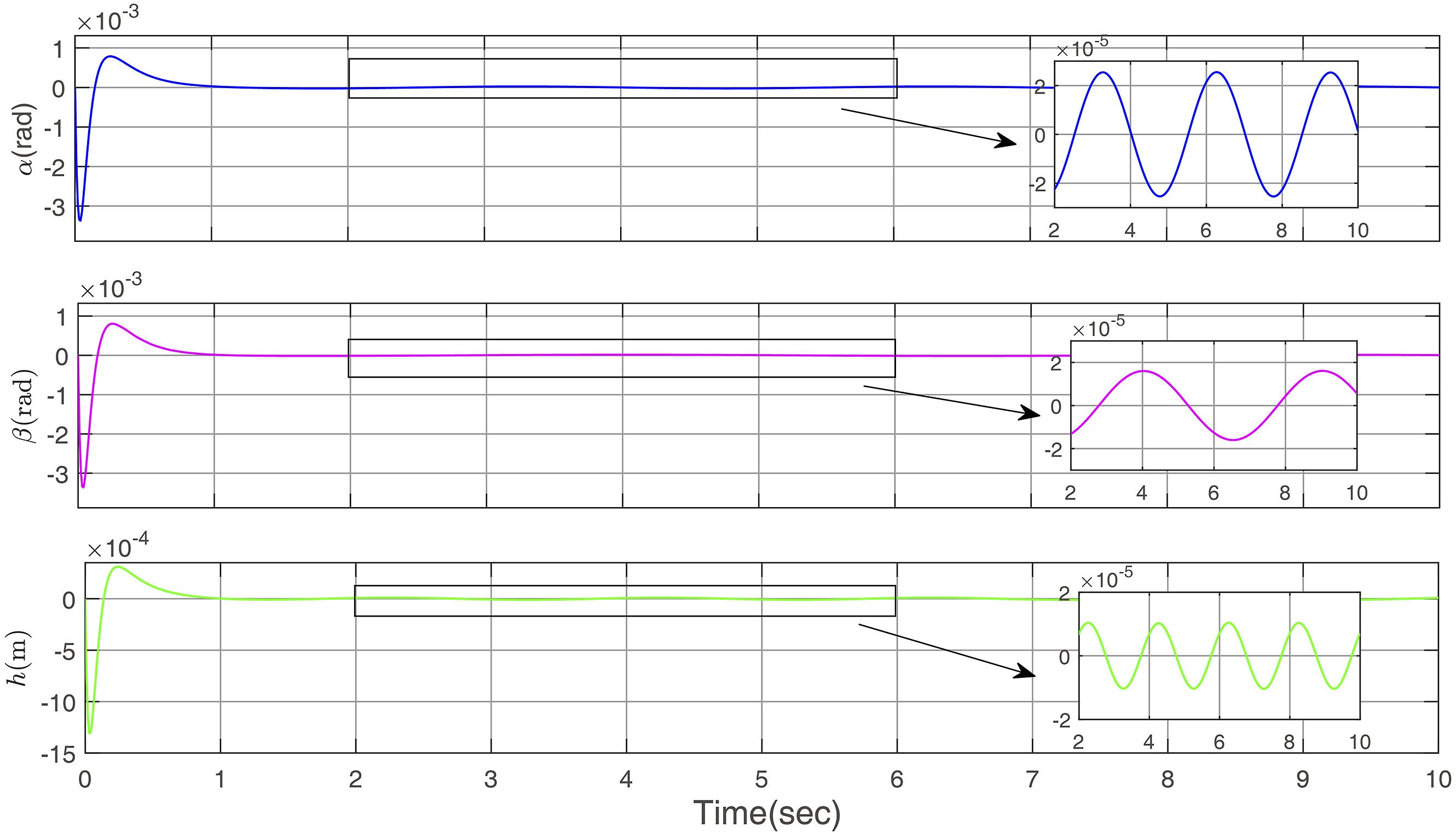
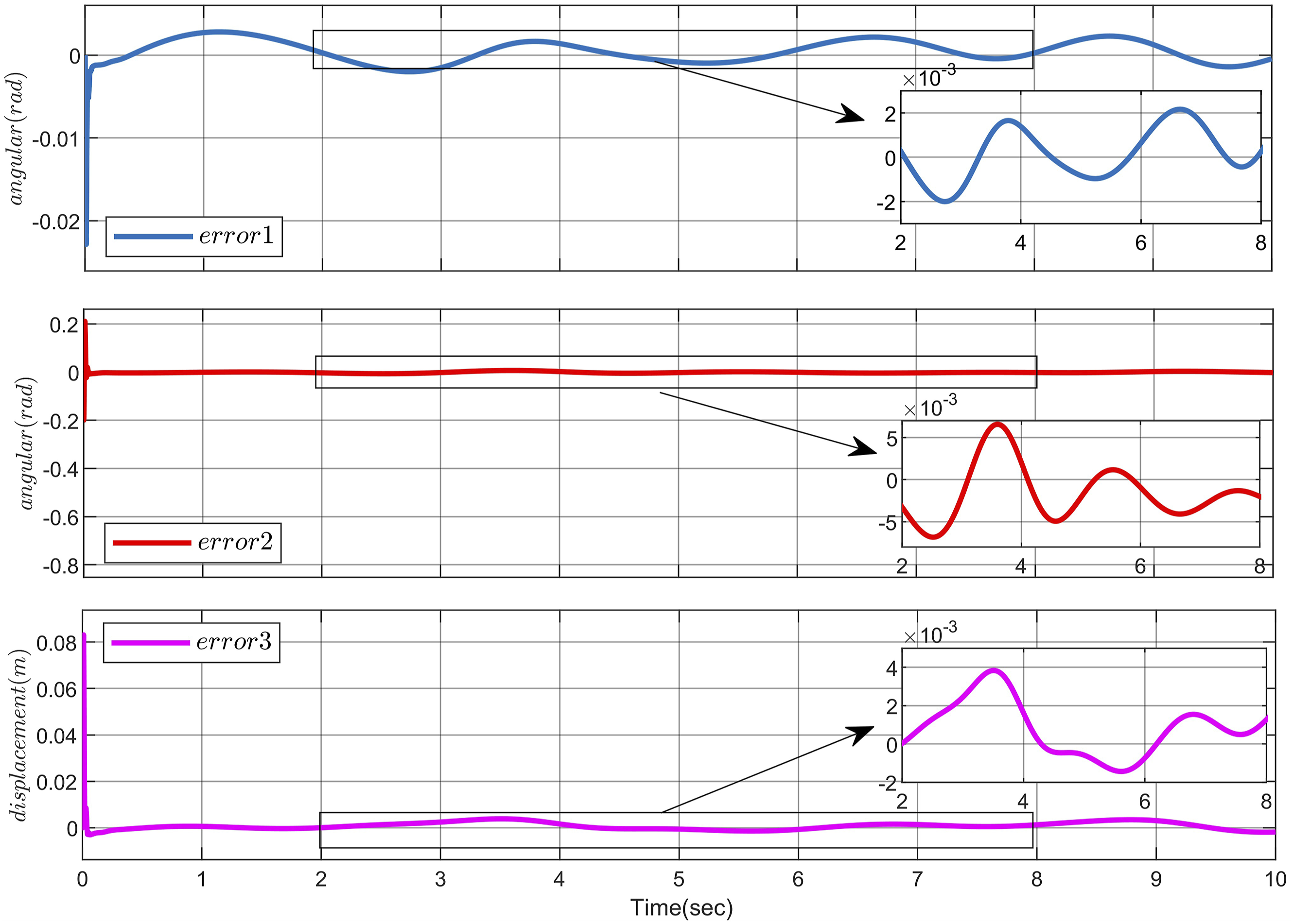
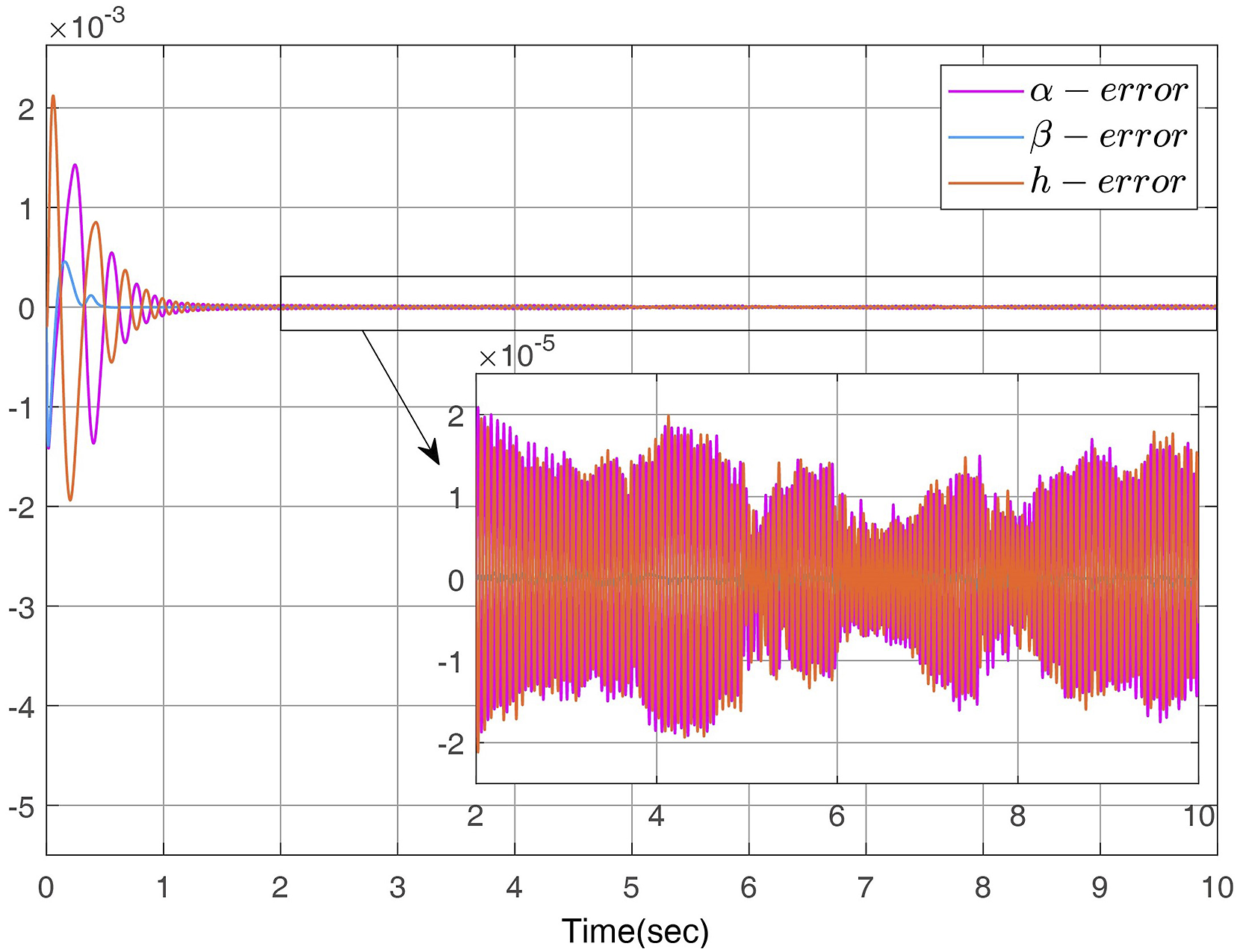
Tracking error curve.

To evaluate the performance of the observer, the tracking curve of the observer to the set disturbance and its error curve are provided, as shown in Figures 7 and 8. The observer can track the disturbance within 0.1 seconds and control the tracking error within the order of 10⁻³, demonstrating its effectiveness. Utilizing the observer can offset the disturbance at the controller level to a certain extent, thereby improving the system’s robustness.

Figure 7.

Observer tracking curve.

Figure 8.

Observer error curve.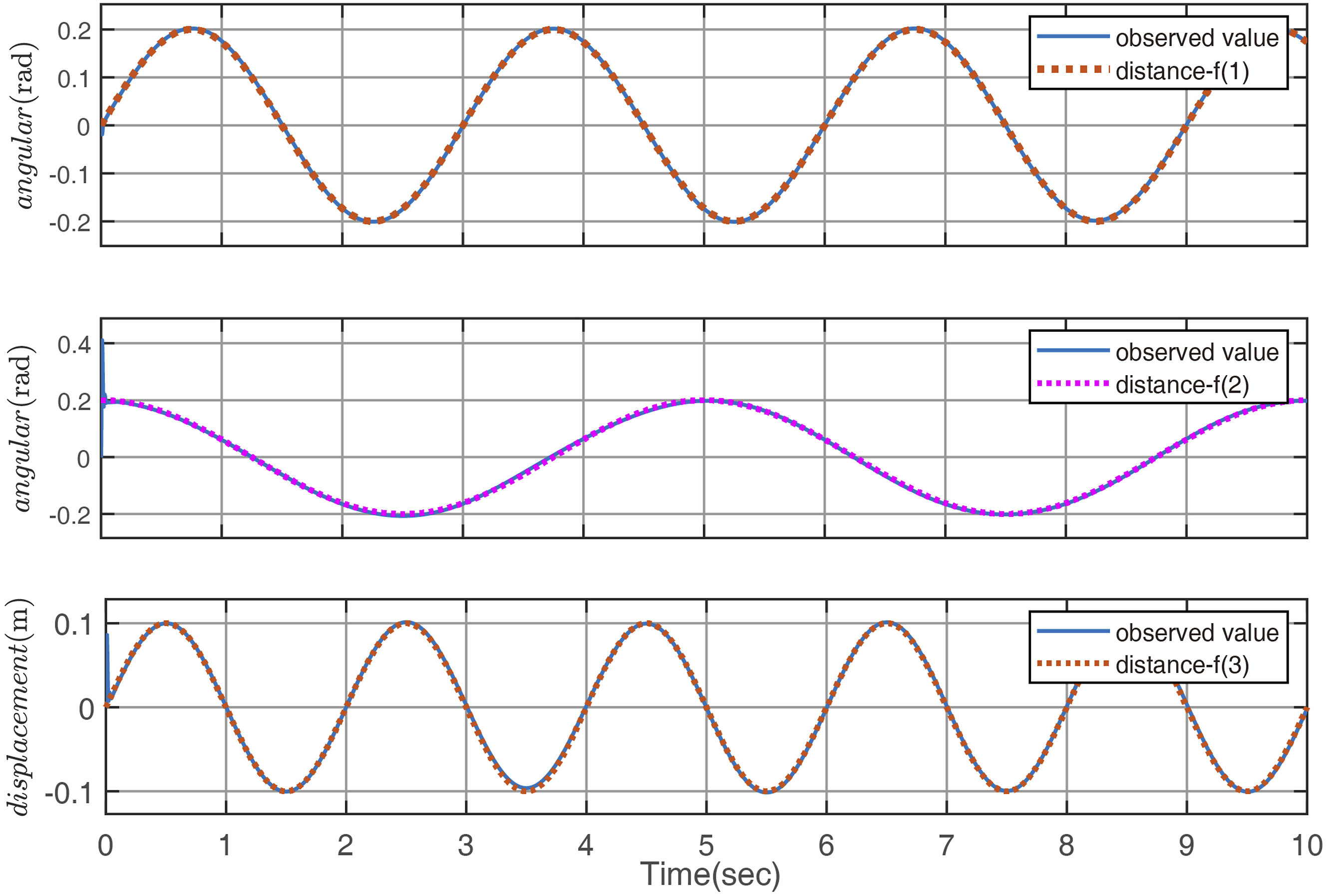

To demonstrate the excellent performance of the hyperbolic convergence law sliding mode control strategy proposed in this study for the parallel robot, we compare it with recent control strategies. Controllers such as the computational torque controller (CTC), fuzzy sliding mode controller (FSMC), and super-twisting sliding mode controller (STSMC) exhibit better convergence speed and control accuracy, respectively. The computational torque controller significantly improves error convergence speed compared to feed-forward PD and simple PID control. Meanwhile, the fuzzy sliding mode controller and super-twisting sliding mode controller are more effective in reducing the jitter and vibration associated with sliding mode control. In traditional sliding mode control, the jitter mainly comes from the discontinuity of the control signal, the fuzzy sliding mode controller ensures that the convergence speed is small near the sliding mode surface and increases when moving away from the sliding mode surface by means of fuzzy rules, and the super-twisting sliding mode avoids the direct use of the high-gain switching function term by the design of convergence law. Instead, it employs a state estimation term and a switching function that is related to the output error magnitude, and this design makes the control signal more continuous and smooth.

Equation (87) illustrates the computational torque controller for the parallel robot. Equation (88) presents the super-twisting sliding-mode controller for the parallel robot, designed based on the super-twisting sliding-mode control strategy. Following Wu et al.’s fuzzy sliding-mode robot controller strategy, we developed the fuzzy sliding-mode controller for the parallel robot, as shown in equation (89). The fuzzy rules are referenced from Wu et al.’s paper (Wu et al., 2021) and will not be elaborated upon here. Fuzzy sliding mode controllers and super-twisting sliding mode controllers are consistent with the sliding mode surface designed in this paper. The relevant controller parameters are shown in Table 2.

F = M (x_{1}) [{\ddot{x}}_{d} - K_{p} e - K_{d} \dot{e}] + C (x_{1}, x_{2}) x_{2} + G (x_{1})

(87)

\{\begin{cases} \dot{s} = - λ {|s|}^{\frac{1}{2}} sign (s) + v \\ v = - α_{1} sign (s) \\ F = C (x_{1}, x_{2}) x_{2} + G \\ + M (x_{1}) [{\ddot{x}}_{1} + k_{d}^{- 1} (\dot{s} - k_{p} \dot{e} - k_{i} e)] \end{cases}

(88)

\{\begin{cases} F_{s w} = K_{s} \cdot s i g n (s) \\ F_{e q} = M (x_{1}) [k_{d} {\ddot{x}}_{1 d} - k_{i} e - k_{p} \dot{e}] + C (x_{1}, x_{2}) x_{2} + G \\ F = F_{e q} + F_{s w} \\ K_{s} = d i a g [k_{1}, k_{2}, k_{3}] \end{cases}

(89)

Table 2.

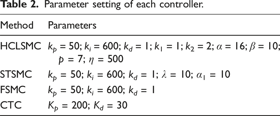
Parameter setting of each controller.

Method	Parameters
HCLSMC	k_p = 50; k_i = 600; k_d = 1; k₁ = 1; k₂ = 2; α = 16; β = 10; p = 7; η = 500
STSMC	k_p = 50; k_i = 600; k_d = 1; λ = 10; α₁ = 10
FSMC	k_p = 50; k_i = 600; k_d = 1
CTC	K_p = 200; K_d = 30

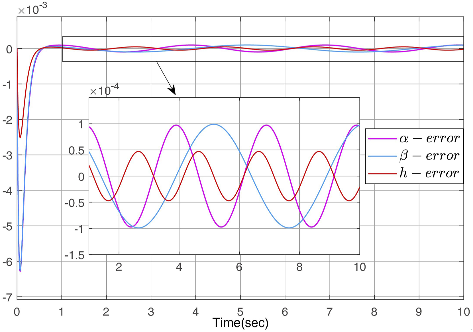
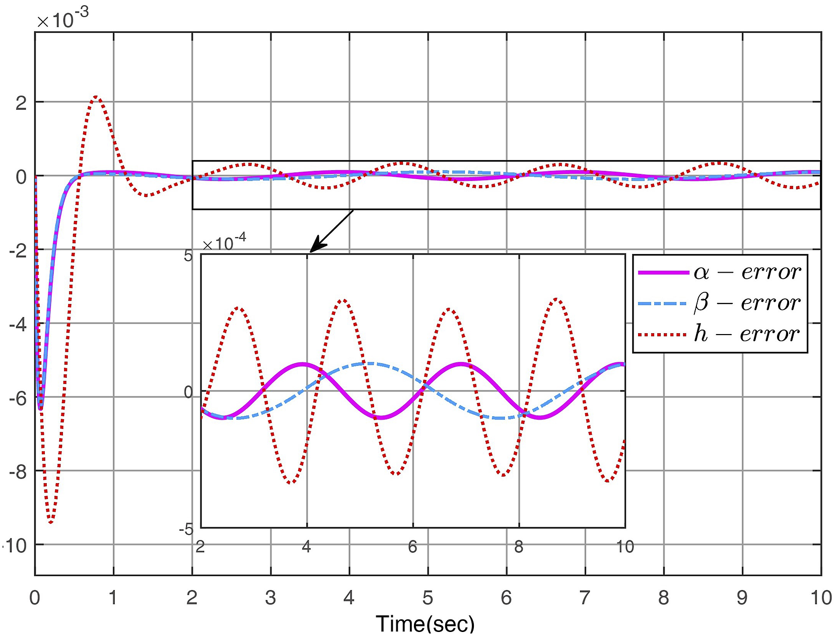
We compare the hyperbolic convergence law sliding mode control strategy proposed in this paper with the three aforementioned control strategies. First, Wu et al.’s fuzzy sliding mode control strategy (Wu et al., 2021) (see Figure 9) exhibits a tracking error of 1 × 10⁻⁴, whereas the control strategy presented in this paper achieves a higher control accuracy with a tracking error of 2 × 10⁻⁵. Furthermore, the controller devised in this study outperforms the fuzzy sliding mode control strategy in terms of speed, converging to a smaller error within 0.3 seconds. When compared to commonly used feedforward PD control and computational torque control methods in robotics (see Figure 10, Figure 11), the control strategy proposed in this paper exhibits substantial enhancements in control accuracy and tracking speed. In contrast to the super-twisting sliding mode control strategy (Dai et al., 2019; Saied et al., 2023) (see Figure 12), the control approach presented here achieves both chattering-free behavior and faster convergence speed without compromising accuracy.

Figure 9.

Fuzzy sliding mode controller tracking error.

Figure 10.

Calculate torque controller error.

Figure 11.

Feedforward PD controller error.

Figure 12.

Super-twisting sliding mode controller error.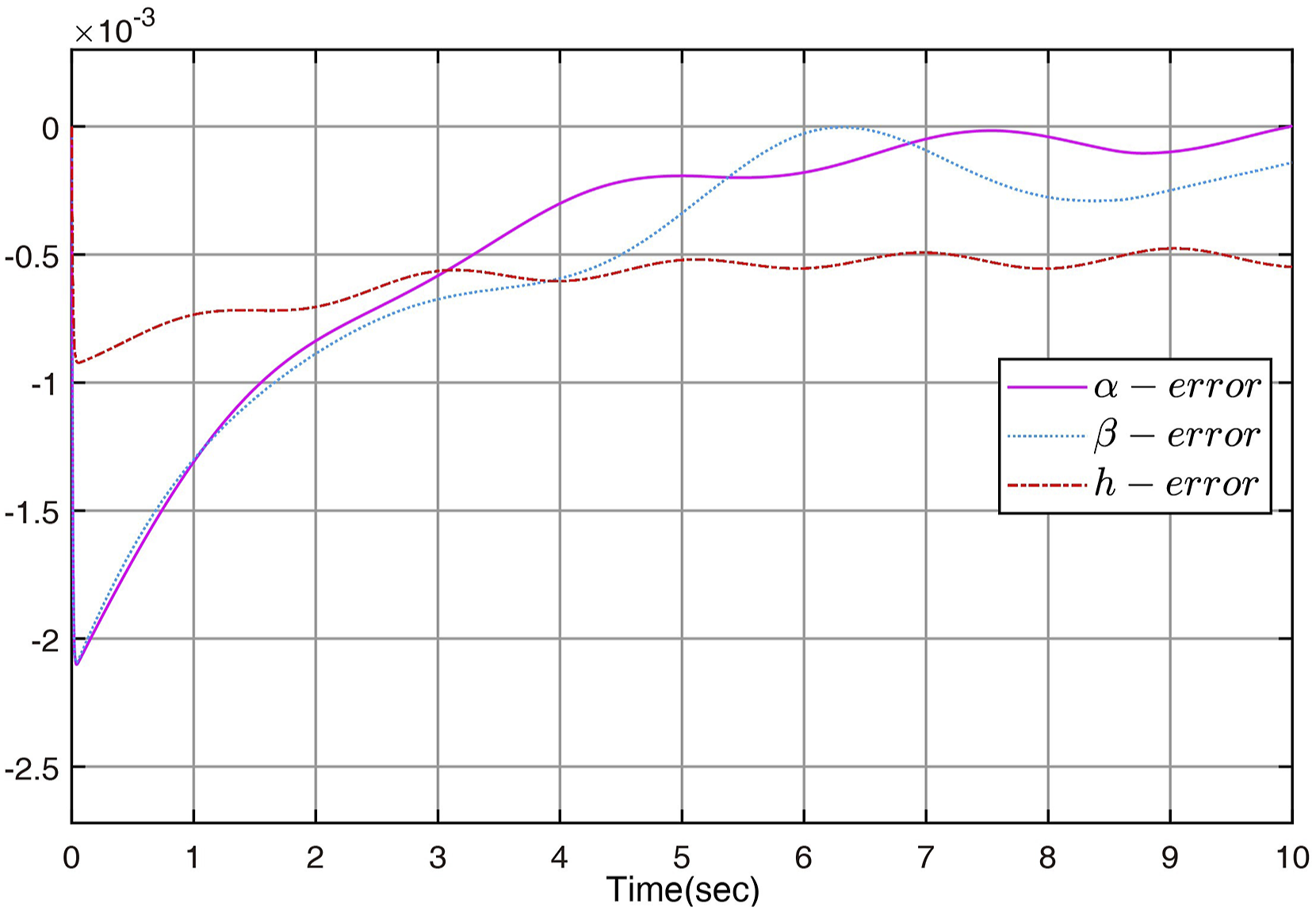

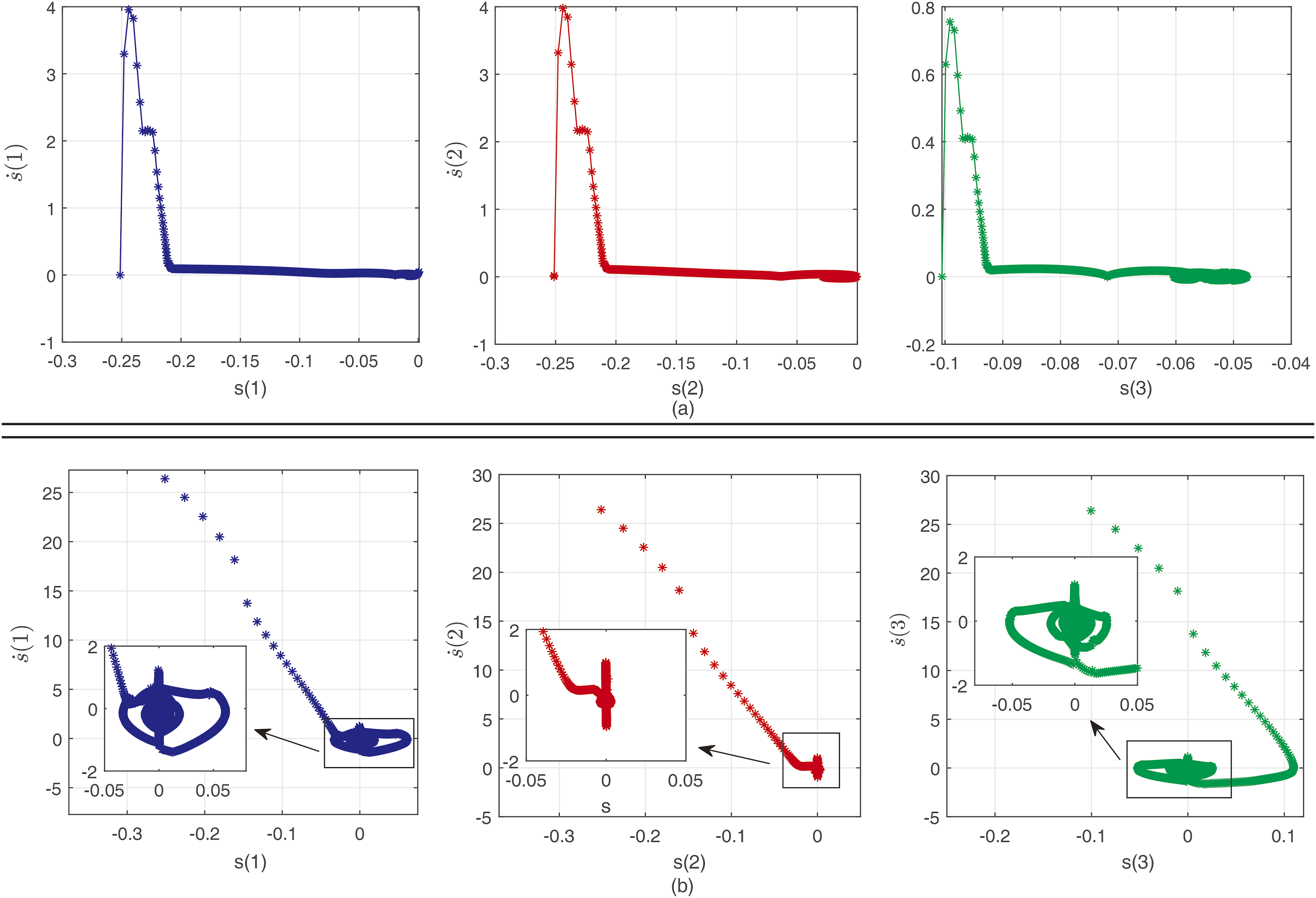
To verify the performance of the parallel robot controller in eliminating chattering, the phase diagram of the sliding mode control based on the hyperbolic convergence law is presented in Figure 13. The control phase diagrams for fuzzy sliding mode control and super-twisting sliding mode control algorithms, which can reduce chattering, are shown in Figure 14. From the phase diagrams, it can be observed that the sliding mode control based on the hyperbolic convergence law exhibits very low speed near the sliding mode surface and no jitter. The slow movement of the sliding variable only causes it to slowly cross the sliding mode surface. The hyperbolic convergence law sliding mode control strategy quickly increases the speed of approaching the sliding mode surface when it is far from it, demonstrating good performance. Although the super-twisting method reduces the amplitude of chattering, some jitter remains, especially near the sliding mode surface, where its approaching speed is larger than that of the hyperbolic convergence law sliding mode control strategy. Therefore, it is less effective in suppressing jitter. The phase diagram also shows that the fuzzy sliding mode can effectively suppress chattering, but the approaching speed becomes very slow when it is not in the smaller neighborhood of the sliding mode surface, affecting the speed of reaching the sliding mode surface. Additionally, the phase diagram indicates that the steady-state neighborhood of the sliding mode control using the hyperbolic convergence law method, when reaching the sliding mode surface, is 0.02. In comparison, the steady-state neighborhoods are 0.2 for the fuzzy sliding mode control and 0.1 for the super-twisting sliding mode control when approaching the sliding mode surface. The hyperbolic convergence law method of sliding mode control, therefore, approaches the sliding mode surface in a significantly smaller neighborhood and maintains stability. This demonstrates the high accuracy of this control strategy. Overall, the sliding mode control based on the hyperbolic convergence law designed in this paper achieves good results in suppressing chattering and reaching speed.

Figure 13.

Hyperbolic convergence law sliding mode control phase diagram.

Figure 14.

(a) Fuzzy sliding mode control phase diagram and (b) super-twisting sliding mode control phase diagram.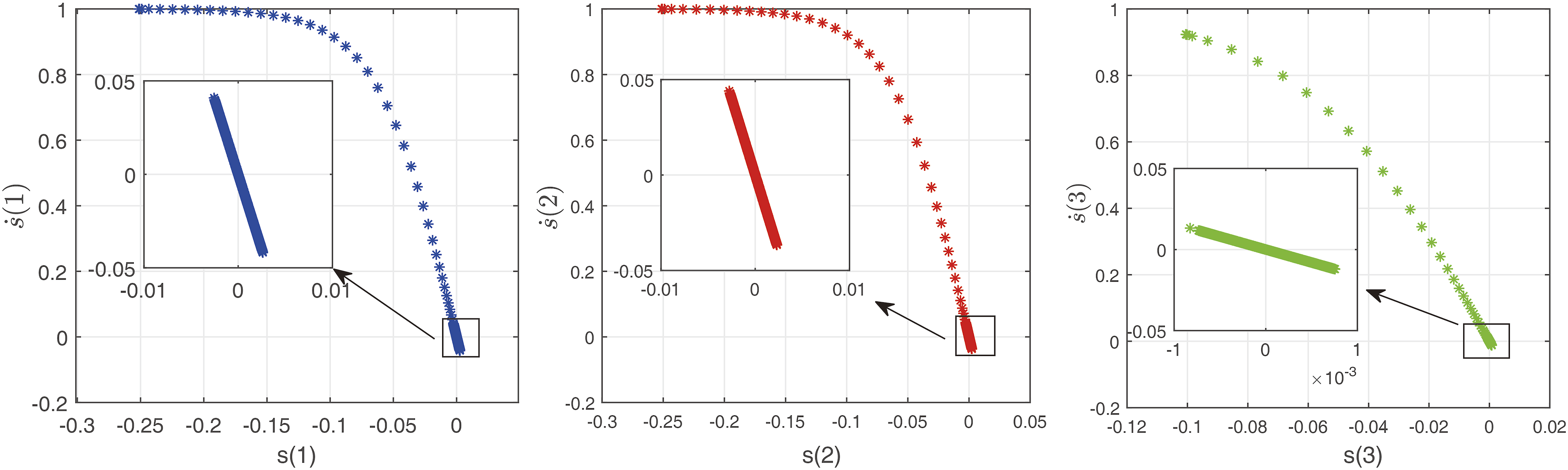

6. Conclusion

This paper introduces an improved dynamic modeling method for parallel robots based on screw theory and the d’Alembert-Lagrange equation, along with a chattering-free sliding mode control strategy. The proposed method calculates inertial wrench using screws and unifies the modeling process for parallel robots. The modeling method can be accomplished by relying on the same set of spin coordinates, which simplifies the modeling process of the parallel robot control problem. The double hyperbolic convergence law sliding mode control method can theoretically and effectively eliminate chattering in sliding mode control, and has the property that the sliding mode variables are closer to the sliding mode surface, which significantly improves the error convergence accuracy and enhances the robustness of the system. Simulation results demonstrate that the sliding mode control strategy based on the hyperbolic convergence law effectively controls the parallel robot, the control accuracy has improved from the order of 10⁻⁴ to the order of 10⁻⁵ compared to control methods with less jitter, such as fuzzy sliding mode control methods, offering advantages in eliminating chattering, reducing tracking error, and improving response speed. Therefore, the proposed screw-based dynamic modeling and sliding mode control strategy effectively meets the precise control requirements of parallel robots.

Footnotes

Declaration of conflicting interests

The author(s) declared no potential conflicts of interest with respect to the research, authorship, and/or publication of this article.

Funding

The author(s) disclosed receipt of the following financial support for the research, authorship, and/or publication of this article: This paper is supported in the National Natural Science Foundation of China under Grant (52375490).

ORCID iD

Fengshuo Zhao

Appendix

References

Abo-Shanab

(2020) Dynamic modeling of parallel manipulators based on Lagrange-D’Alembert formulation and Jacobian/Hessian matrices. Multibody System Dynamics 48(4): 403–426.

Lee

, et al. (2017) Geometrical kinematic solution of serial spatial manipulators using screw theory. Mechanism and Machine Theory 116: 404–418.

Asker

Assal

El-Bab

AMF

(2014) Dynamic modeling of a parallel manipulator-based mobility assistive device for elderly people. In: 22nd Mediterranean Conference on Control and Automation. Piscataway: IEEE, 362–367.

Bidard

(1993) Screw-vector bond graphs for multibody systems modelling. Simulation Series 25: 195.

Chen

, et al. (2017) A new approach for the identification of reciprocal screw systems and its application to the kinematics analysis of limited-DOF parallel manipulators. Mechanism and Machine Theory 118: 194–218.

Cheng

Yuan

, et al. (2022) Dynamic modeling method of multibody system of 6-DOF robot based on screw theory. Machines 10(7): 499.

Cibicik

Egeland

(2019) Dynamic modelling and force analysis of a knuckle boom crane using screw theory. Mechanism and Machine Theory 133: 179–194.

Condurache

(2022) Higher-order relative kinematics of rigid body and multibody systems. A novel approach with real and dual lie algebras. Mechanism and Machine Theory 176: 104999.

Dai

Rees Jones

(2001) Interrelationship between screw systems and corresponding reciprocal systems and applications. Mechanism and Machine Theory 36(5): 633–651.

10.

Dai

Cheng

(2019) Super-twisting sliding mode control design for electric dynamic load simulator. In: 2019 Chinese Control Conference (CCC). Piscataway: IEEE, 3078–3083.

11.

Yang

(1988) Inverse dynamic analysis and simulation of a platform type of robot. Journal of Robotic Systems 5(3): 209–227.

12.

Dong

Liu

Xiao

, et al. (2021) Dynamic modeling and design of a 5-DOF hybrid robot for machining. Mechanism and Machine Theory 165: 104438.

13.

Gallardo

Rico

Frisoli

, et al. (2003) Dynamics of parallel manipulators by means of screw theory. Mechanism and Machine Theory 38(11): 1113–1131.

14.

Gallardo-Alvarado

Aguilar-Nájera

Casique-Rosas

, et al. (2008) Kinematics and dynamics of 2(3-RPS) manipulators by means of screw theory and the principle of virtual work. Mechanism and Machine Theory 43(10): 1281–1294.

15.

Gallardo-Alvarado

Rodríguez-Castro

Delossantos-Lara

(2018) Kinematics and dynamics of a 4-PRUR Schonflies parallel manipulator by means of screw theory and the principle of virtual work. Mechanism and Machine Theory 122: 347–360.

16.

Gosselin

(1995) Simulation and computer-aided kinematic design of three-degree-of-freedom spherical parallel manipulators. Journal of Robotic Systems 12(12): 857–869.

17.

Zhang

, et al. (2022) Cascade sliding mode control of four-sided clamped plate based on extended state observer. In: 2022 IEEE 11th Data Driven Control and Learning Systems Conference (DDCLS). Piscataway: IEEE, 222–226.

18.

Guo

Song

(2015) Screw bond graph in the application of the parallel mechanism dynamics modeling. Journal of Mechanical Engineering 51(23): 12–20.

19.

Huang

Liu

Chetwynd

(2011) Generalized Jacobian analysis of lower mobility manipulators. Mechanism and Machine Theory 46(6): 831–844.

20.

Kardos

(2019) Robust computed torque method of robot tracking control. In: 22nd International Conference on Process Control (PC19). Strbske Pleso, Slovakia: IEEE, 102–107.

21.

Levant

(1993) Sliding order and sliding accuracy in sliding mode control. International Journal of Control 58(6): 1247–1263.

22.

(2004) Control performance improvement of a parallel robot via the design for control approach. Mechatronics 14(8): 947–964.

23.

(2022) Sliding-mode nonlinear predictive control of brain-controlled mobile robots. IEEE Transactions on Cybernetics 52(6): 5419–5431.

24.

Lynch

Park

(2017) Modern Robotics. Cambridge: Cambridge University Press.

25.

Zhang

Liu

, et al. (2018) Bond graph-based dynamic model of planetary roller screw mechanism with consideration of axial clearance and friction. Proceedings of the Institution of Mechanical Engineers - Part C: Journal of Mechanical Engineering Science 232(16): 2899–2911.

26.

Merlet

(2005) Jacobian, manipulability, condition number and accuracy of parallel robots. In: 12th International Symposium on Robotics Research (ISRR). San Francisco, CA; Springer, 175–184.

27.

Nguyen

Cheah

(2022) Analytic deep neural network-based robot control. Ieee-Asme Transactions on Mechatronics 27(4): 2176–2184.

28.

Qiu

Dai

Qiu

, et al. (2021) An introduction to screw theory. In: Analysis and Synthesis of Compliant Parallel Mechanisms—Screw Theory Approach. Berlin, Germany: Springer Nature, 17–31.

29.

Saied

Chemori

Bouri

, et al. (2023) FeedForward super-twisting sliding mode control for robotic manipulators: application to PKMs. IEEE Transactions on Robotics 39(4): 3167–3184.

30.

Tao

Chen

Nan

, et al. (2018) Double hyperbolic reaching law with chattering-free and fast convergence. IEEE Access 6: 27717–27725.

31.

Tsai

L-W

(1999a) Solving the inverse dynamics of a Stewart-Gough manipulator by the principle of virtual work. Journal of Mechanical Design 122(1): 3–9.

32.

Zhang

Zhu

, et al. (2021) Fuzzy sliding mode variable structure control of a high-speed parallel PnP robot. Mechanism and Machine Theory 162: 104349.

33.

Xiao

Wang

Tian

, et al. (2024) A novel adaptive robust control for trajectory tracking of mobile robot with uncertainties. Journal of Vibration and Control 30(5-6): 1313–1325.

34.

Zhao

Zhong

(2024b) Active and passive heave compensation system based on feedback linearization sliding mode variable structure control. Ocean Engineering 305: 117962.

35.

Zhao

Zhong

Wang

, et al. (2024a) Multi-motor average deviation coupling control strategy based on hyperbolic convergence law high-order sliding mode control using extended state sliding mode observer. Journal of Vibration and Control. Epub ahead of print 12 April 2024. DOI: 10.1177/10775463241246323.