An 1D-3D coupling method for flow-induced vibration of pump-valve-pipe system

Abstract

The flow-induced vibration (FIV) in ship pump-valve-pipe system is characterized by significant coupling effects between components. However, due to the presence of multiple excitation sources and cross-scale mesh challenges, traditional FIV calculation methods prove inadequate for system-level simulation. To overcome this limitation, a system-level FIV simulation interface program was developed in this study. Using a partitioned excitation extraction approach, the FIV loads for the system were calculated and applied to the structural dynamics model. Ultimately, a computational method for system-level FIV simulation based on a 1D-3D coupling algorithm was developed. To validate the accuracy, an experiment was conducted. The results demonstrate that this methodology significantly improves the computational efficiency of system-level flow-induced vibration simulations while maintaining satisfactory accuracy. Furthermore, the FIV of system during the valve closing process is simulated, and the transient vibration characteristics were investigated. Additionally, the influence of valve closing time and mode on the flow field and vibration characteristics of the pump was investigated. The pump head exhibits an oscillating increase during the valve closing process, while the vibration in the impeller’s radial direction intensifies with decreasing flow rate.

Keywords

1D-3D coupled pump flow-induced vibration system-level simulation piping system

1. Introduction

There are many pipes and equipment connected to each other to form a variety of piping systems on the ship. The piping system is usually composed of pumps, valves, pipes, and other accessories. It is mainly used to transport the fluid medium on the ship for the ship’s proper performance, which is a very essential work in the ship. The transient effects on the flow of entire system are induced when operational conditions are switched or unexpected malfunctions of components occur, thereby leading to abnormal vibrations (Kong et al., 2014). The vibration of an individual component is frequently transmitted to other components through pipelines, thereby generating coupling effects. These coupling effects include Poisson coupling (Tijsseling and Vardy, 2004; Zhang et al., 1999), junction coupling (Ahmadi and Keramat, 2010; Heinsbroek, 1997), and Bourdon coupling (Adamkowski et al., 2010; Chen, 2012; Whatham and F, 1987), among others. Under the influence of such coupling effects, resonance may be induced, leading to further deterioration of system vibrations. However, simulations of individual components fail to account for inter-component coupling, which can only be considered in system-level simulations.

Previous studies of flow-induced vibration (FIV) in piping systems have often focused on single components, such as pipe sections (Askarian et al., 2020; Durant et al., 2000; Pittard et al., 2004; Ryu et al., 2004; Stangl and Irschik, 2005; Zhang et al., 2015; Zhao and Sun, 2018), pumps (W J Guo, 2017; J H Wang et al., 2019; J Fei, 2013; Jiang et al., 2007; Guo et al., 2023), and valves (Domnick and Brillert, 2019; Misra et al., 2002; Yonezawa et al., 2012; Zeid and Shouman, 2019). For pipe sections, Li Kun et al. (K Li et al., 2007) analyzed the flow field within a single pipe and obtain flow-excited load acting, which was applied in structural dynamics model to carry out FIV analysis. Li et al. (Li et al., 2019) established the fluid-structure interaction dynamic equations of a cantilevered pipe system based on the Euler–Bernoulli beam theory, through which the vibrational response of the piping system was calculated, ultimately leading to the proposal of an effective control strategy. According to the review by Ding and Ji (Ding and Ji, 2023) and the studies on fluid-conveying pipelines by Gao et al. (Gao et al., 2020, 2021), vibration control in integrated pipeline systems remains a challenging issue. However, due to the large number of pipelines in such integrated systems, accurate numerical simulation proves particularly difficult to achieve. For pumps, Zhao et al. (Zhao and Chai, 2024), Benra (Benra, 2006), and Zhang et al. (Zhang et al., 2020) conducted studies on the vibroacoustic characteristics of pumps using a single pump as the research subject. The results indicate that the dominant frequencies are primarily associated with the blade-passing frequency. Guo et al. (Guo et al., 2023) and Xue et al. (Xue et al., 2024) investigated the vibration characteristics of pump-turbine units under conditions considering component interactions. Their research demonstrates that, like the abnormal vibration observed in turbine head covers, coupled vibration effects exist among components. As for valves, Yonezawa et al. (Yonezawa et al., 2012) and Domnick et al. (Domnick and Brillert, 2019) studied the mechanism of vibration for different by experiments and numerical simulations. Simulations by Misra et al. (Misra et al., 2002) showed that the occurrence of self-excited vibrations was caused by a combined effect of water hammer, downstream piping acoustic feedback, high acoustic resistance, and adverse hydraulic stiffness at the control valve. It can be illustrated that the coupling effect between equipment is not negligible in piping systems.

The aforementioned studies demonstrate that the majority of existing research has focused solely on the individual effects of single components, failing to account for the intricate coupling interactions among all components within the entire system (Ahmed et al., 2022). In contrast, another subset of studies that consider limited component coupling further reveals that the vibration response induced by resonance from such interactions cannot be neglected (Guo et al., 2023; Misra et al., 2002; Qing et al., 2006; Xue et al., 2024). However, when addressing the comprehensive coupling effects among all components throughout the entire pipeline system, current methodologies prove inadequate for computational analysis. Consequently, it is imperative to develop a system-level computational approach specifically designed for global pipeline systems.

Although there are fewer system-level simulations on FIV, there have been several studies on the flow field for system-level (Papukchiev and Lerchl, 2012; Viel et al., 2010; Yan, 2011). System-level flow field simulation is typically based on a coupled solution approach integrating three-dimensional (3D) Computational Fluid Dynamics (CFD) and the one-dimensional (1D) Method of Characteristics (MOC). Ljubijankic et al. (Ljubijankic et al., 2013) proposed a hybrid system modeling approach and simulated a building energy supply system. Liu et al. (Q L Liu, 2013; Wu et al., 2012) analyzed the flow characteristics within circulating pipes using the coupled simulation method based on an interface between Flowmaster and Fluent. Yang et al. (S YANG, 2015) investigated the transient flow characteristics of pumping piping system using CFD-MOC method and verified the precision of coupled method by experiment. Al-Khomairi (Al and A, 2003) and Li et al. (Li et al., 2023) have also investigated the flow characteristics of pump-valve-pipeline systems by experiments and simulations. However, research remains limited regarding system-level FIV load application and coupling effects in vibrational analysis.

These researches demonstrate that significant coupling effects exist in FIVs among system components, and only through system-level simulation can the FIV characteristics of the entire pipeline system be accurately analyzed. However, current research in this area remains notably limited, primarily due to two key challenges: (1) Traditional coupling algorithms involve numerous 1D components, making it difficult to extract flow excitation sources from all critical excitation components across the system; (2) The accurate application of multi-source flow excitations to the FIV structural dynamics model presents considerable difficulties. To address these issues, this study develops a partitioned excitation extraction strategy and a fluid-structure interaction interface program. This approach enables the application of multi-source, cross-scale flow excitation sources and advances system-level FIV analysis methodology.

2. Experimental and numerical simulation methods

This section presents experiments on pump-valve-pipe systems and coupled method for flow and FIVs. Simulation based on the method are carried out, and the results are compared with the experiments to verify the accuracy. Since the primary contribution of this paper is the coupled method, only the method is described here. More detailed theoretical part can be found in Appendix.

The coupling method of the pipeline system is implemented as follows: a 3D method is applied on key components in the system, while a 1D method is used for other components. Boundary conditions are provided to each other at the interface to transfer boundary information. When considering the pump as a key component to extract the excitation sources, the pump is simulated by the 3D method, and others are simulated by the 1D method. The working point of the pump in the system is found by multiple iterations of the data exchange between pump and the pipe at the boundary. An initial velocity V1 for pump at the boundary is given, and the corresponding pressure is obtained by the 3D method. This pressure is then transferred as a boundary condition to the 1D calculation to get the velocity V2. The convergence of the flow rate obtained by iterative calculation is judged. If it does not converge, the boundary conditions are updated and the 3D calculation is performed until the stable working point of the pump in the system is found.

2.1. Experiments

The experimental setup is illustrated in Figure 1, comprising a pump, valves, inlet pipes, and other components. Accelerometers were mounted on the pump foot, volute outer surface, as well as at the inlet and outlet positions to measure vibration. Rated flow rate of pump is 150 m³/h, lift is 27 m, rotational speed is 2950 r/min, and diameter is 100 mm. After achieving stable operation, the flow rate is adjusted using the valve on the discharge end of the pump. Acceleration is collected when the flow rate is 100 m³/h, 120 m³/h, 150 m³/h, and 180 m³/h. Detailed experiment can be found in our previous studies (Zhou et al., 2023).

Figure 1.

Schematic diagram of pump-valve piping system experimental device: (a) schematic diagram and (b) physical model.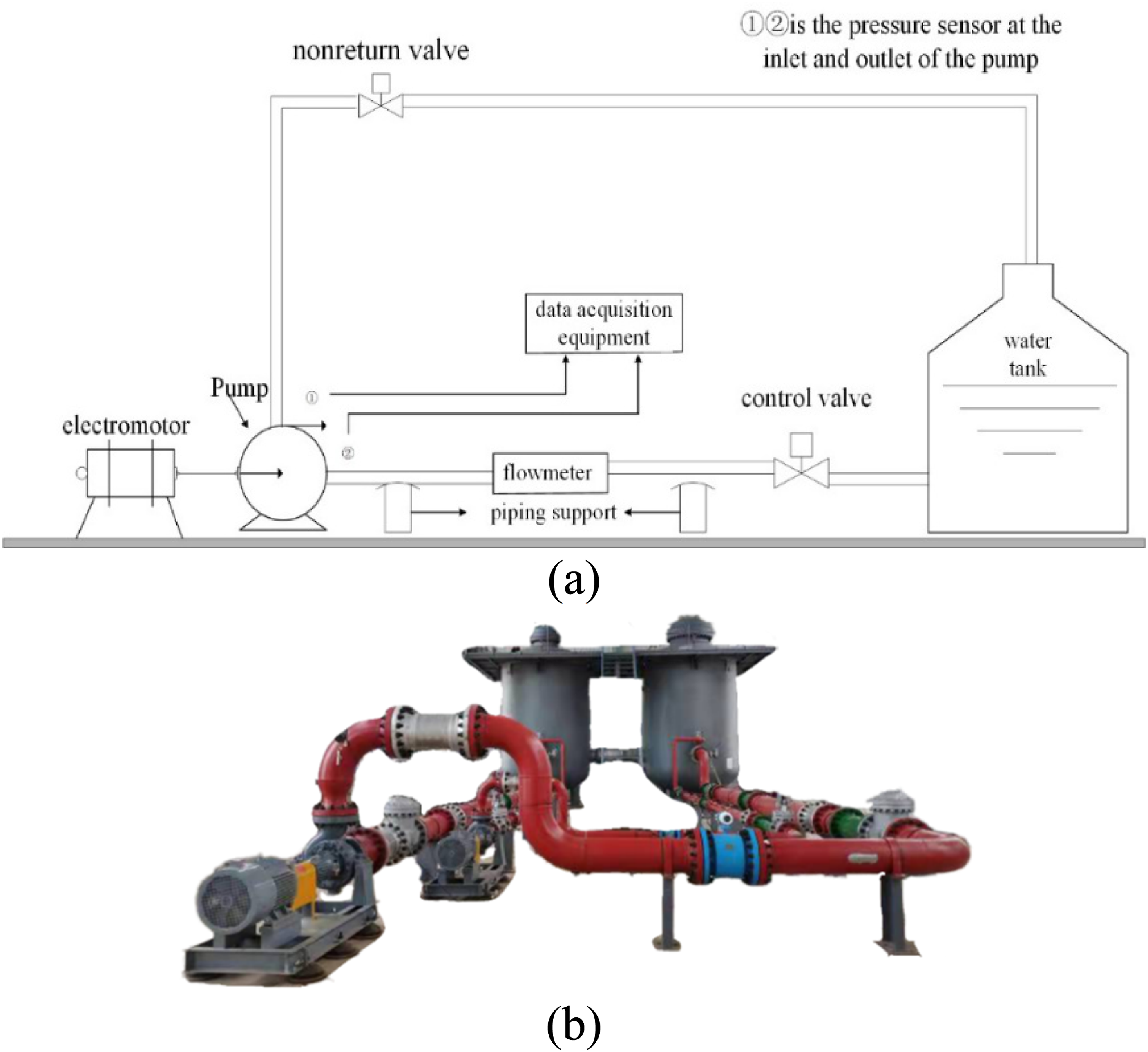

2.2. Coupled numerical simulation method for flow fields

When the 3D method is applied to pipe system, the cost is huge. Although the computational cost is small while the 1D calculation is adopted, it is impossible to visualize and analyze inner flow conditions or to provide excitation. The 1D-3D coupled method can provide load information for FIV under the premise of reducing computational costs. In this paper, the 1D software Flowmaster and the 3D software FLUENT are used to process loads on system using a block extraction-simultaneous loading strategy, that is, 1D-3D coupled flow field computation method is applied to extract the excitation sources of different components separately. Then a secondary development interface program is used to apply the loads to the whole dynamics model of the pipe system. The FIV is performed based on the ANSYS APDL.

When extracting the excitation for a component, that component is modeled using the 3D method to obtain detailed load information. The remaining components are simulated using the 1D method to reduce costs. The components selected for excitation extraction are pumps, valves, and pipes. A total of three coupled simulations are carried out. The fluid meshes of the pump and valve are presented in Figure 2, with 4,081,790 and 2,870,426 elements, respectively.

Figure 2.

Fluid mesh for pumps and valves: (a) pumps and (b) valves.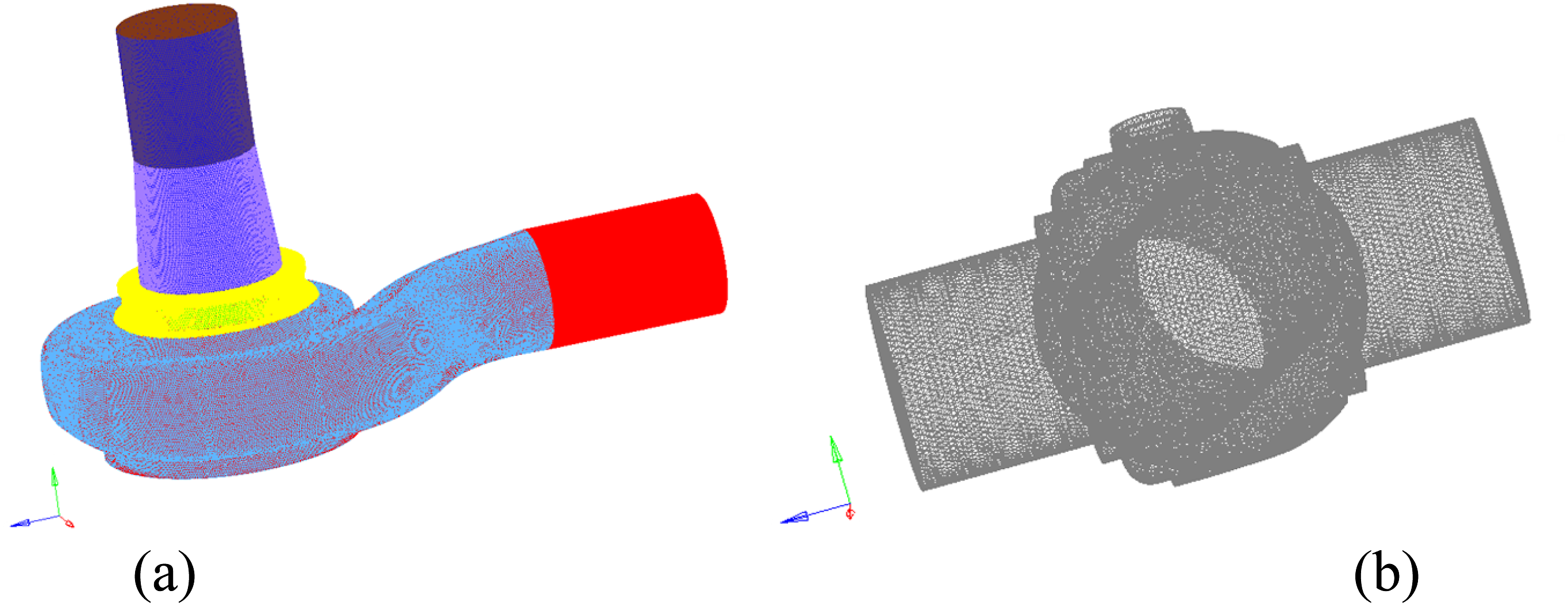

To illustrate the coupled calculation method, the pump is selected as the component for extraction. The pump is calculated using the mesh shown above, while the remaining components are modeled as shown in Figure 3. In the 1D model, the pump is replaced by two pressure components. The simulation begins with a steady-state coupling analysis, the results of which serve as the initial conditions for the transient simulation. For 3D transient simulation, a time step of 2 degrees of blade rotation is adopted, along with the Smagorinsky–Lilly model. The same time step is used for 1D simulation. After the time sub-steps of the 3D calculation have converged, the pressure of the inlet and outlet is obtained and transferred to the 1D model using the interface program. The 1D simulation of the whole pipe is then performed to obtain flow information for components 1 and 7 in Figure 3, which are fed back into the 3D pump model to advance the solution in time.

Figure 3.

Coupled calculation model of piping system (with pump as extracted component).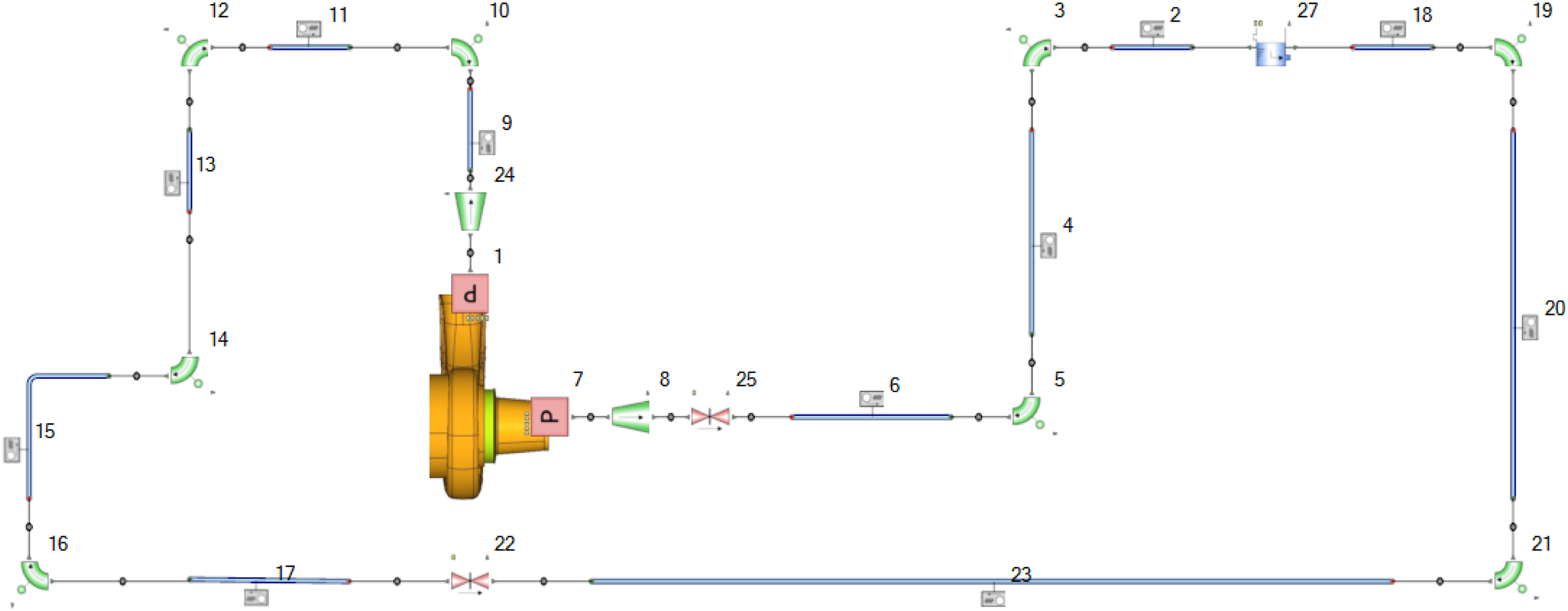

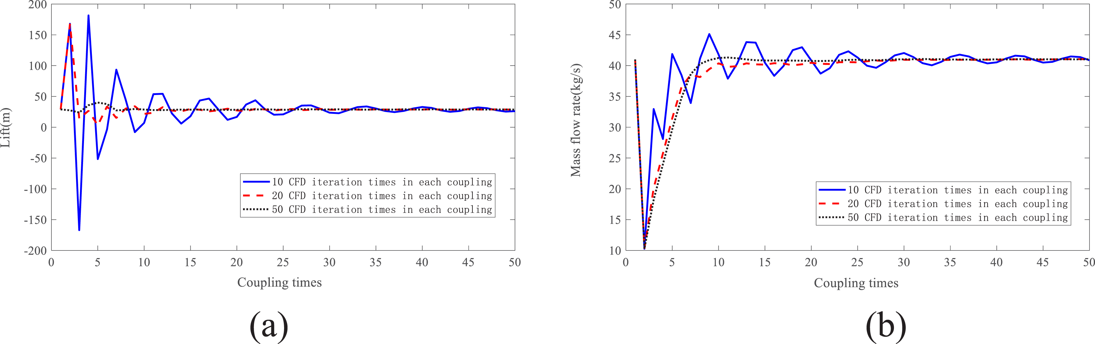
The relaxation factor (α)in the 1D calculations and the number of iterations per time sub-step in the 3D calculations significantly influence the simulations. To optimize accuracy, these parameters were systematically investigated. Four different α were used for the coupled simulation displayed in Figure 4. The convergence speed improves with the increase of α, but the instability of the convergence process also increases. When α is too large, it is very likely to diverge. Based on a balance between convergence speed and stability, α = 0.3 was selected for subsequent analyses. Figure 4 also reveals that time-varying flow rates at the boundary exacerbate convergence challenges. Even a single divergence event in the coupling process can destabilize the CFD solution. Therefore, three different CFD iteration counts were evaluated to determine the optimal number between stability and computational cost in Figure 5. Increasing the number of CFD iterations enhances convergence stability but prolongs simulation time. After analysis, 20 iterations per step were chosen as the optimal number.

Figure 4.

Flow rate of pump with α: (a) by CFD and (b) by MOC.

Figure 5.

Variation of pump flow characteristics with iteration times: (a) lift and (b) flow rate.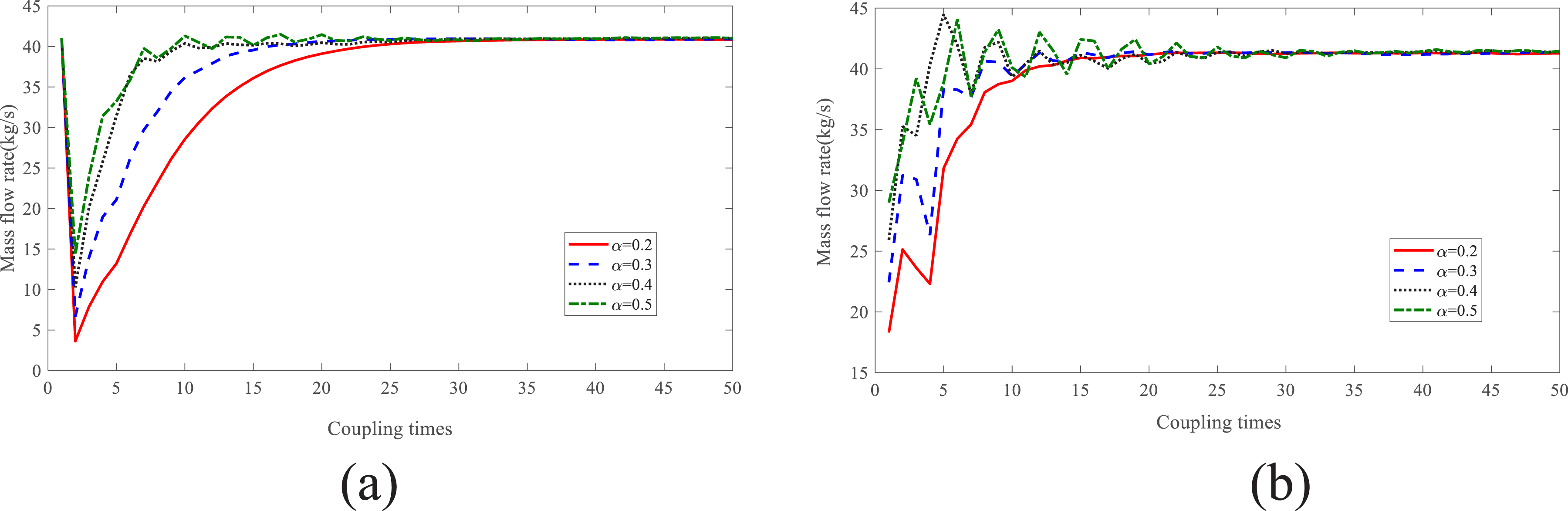

2.3. Coupled numerical simulation method for FIV

The 3D CFD simulations are performed sequentially on each component from which the loads are extracted. The hydraulic loads acting on the pipe system are extracted in pieces. Then the structural dynamics model of system is built, with appropriate constraint boundary conditions applied. Finally, the loads of different components are added onto structure through secondary development interface of the fluid-structure interaction software, enabling FIV analysis. This method can ensure the systematic calculation, fully consider mutual influence between the components, and realize the large-scale calculation of FIV of pipe systems with many complex spatial distributions. By extracting pulsating pressures from multiple excitation sources simultaneously, computational efficiency is significantly improved.

Meshes of structures are shown in Figure 6, which mainly includes pump, valve, pipes, tanks, and other structures. The pump and valve are discretized by the solid unit SOLID185. The pipes and water tank are discretized by the shell unit SHELL181. Impeller is simplified to be a mass point at the center of gravity. Pump shaft is simplified to be a beam unit. Bearings and couplings are stiffness-equivalent using spring units. In addition to the structural mesh, the fluid medium is discretized by a solid mesh, and the cell type is FLUID30, which is coupled with the structural through SURFACE154.

Figure 6.

The FIV finite element mesh for pipes and tanks.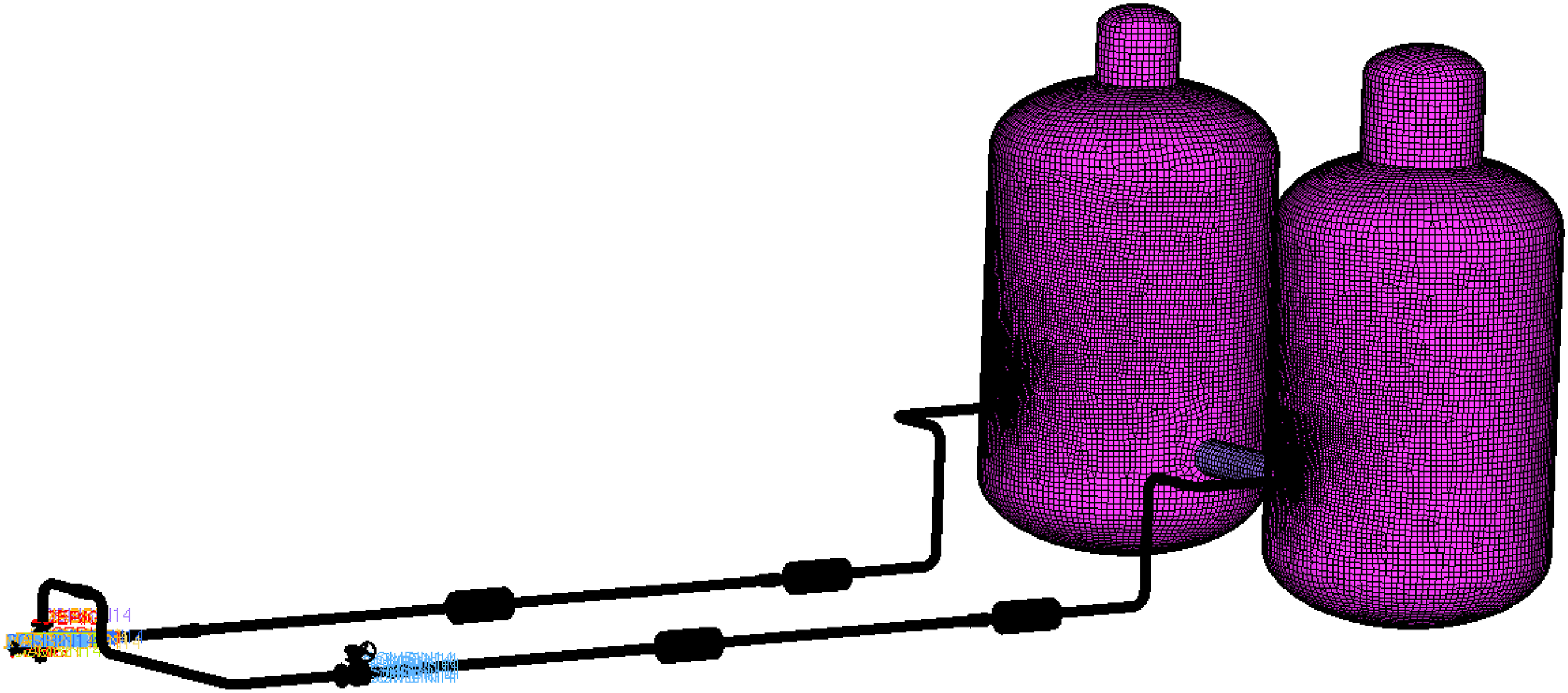

The flow and vibration results were separately validated to ensure accuracy. Following the determination of optimal α and iteration steps, the simulated flow field results were compared with experiment in Figure 7(a). The flow-lift curve of pump exhibits good agreement with the experimental values, confirming the accuracy of the 1D-3D coupled method. The fluid-induced vibration excitation was extracted from the results, and the vibration response was further validated, as showed in Figure 7(b). The simulated acceleration results correlate well with experimental data, with peak values accurately captured, demonstrating the reliability of the method. This methodology achieves a significant reduction in costs for system-level fluid-induced vibration while maintaining computational accuracy.

Figure 7.

Comparison of lift between 1D-3D coupled and experiment: (a) lift and (b) vibration acceleration level.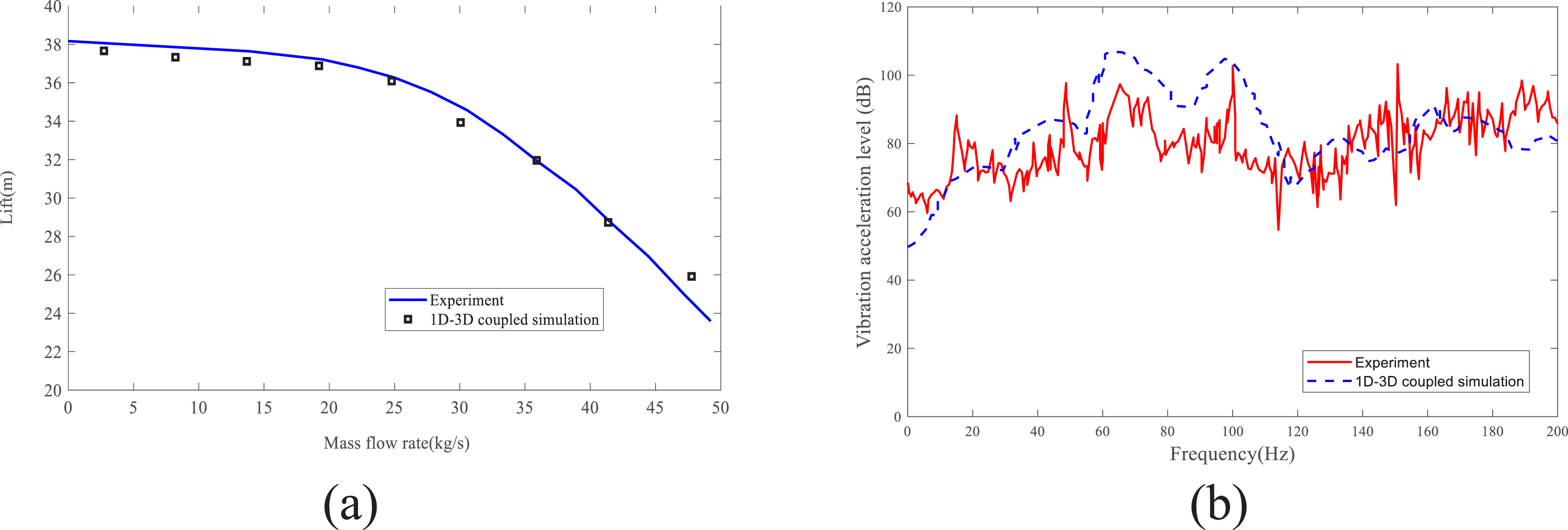

3. Results and discussion

3.1. Single component vs. coupled simulation

When simulating the flow field of a single component, the boundary conditions are usually specified, which cannot capture the fluctuations due to flow changes in the system. The 1D-3D method can capture the pulsation of pressure and flow at the boundary. Figure 8 shows results for flow and pressure at coupled boundary of system obtained by 1D-3D method. Boundary conditions at coupled boundary are pulsating with time, which is more realistic than the constant boundary conditions in the simulation of a single component and can account for effect of system-wide fluctuations on components.

Figure 8.

Results of pressure and mass flow rate at the coupled boundary of the piping system: (a) pressure and (b) mass flow rate.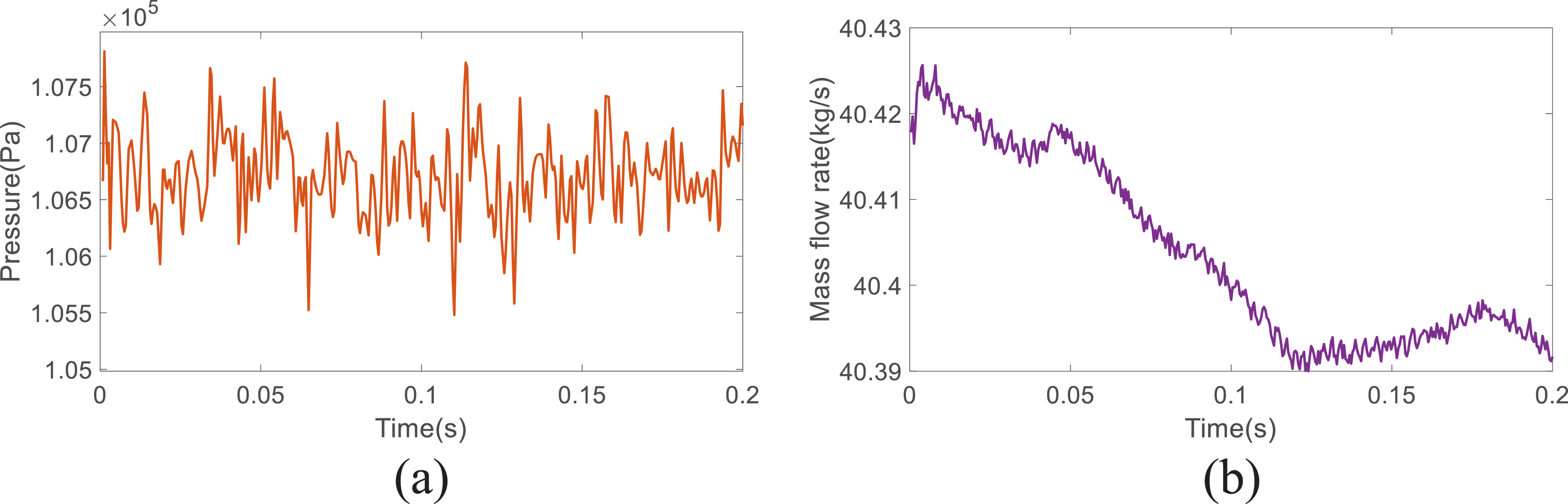

The pump is the source of flow-induced load on an entire system. Fluid in the water tank gains pressure energy when passing through the pump. Due to dynamic and static perturbations inside pump, pressure shows obvious pulsation characteristics. The main pressure loss occurs at the valve downstream of the pump outlet, making the valve the main resistance element in the pipeline system. In addition, due to the inertia and compressibility in fluid as well as elasticity and roughness in wall, additional pressure loss occurs along the pipeline. As with the above phenomena, 1D-3D coupled method provides more realistic results when calculating FIV responses. Figure 9 compares pipeline vibration calculated using a single-component approach and the coupled method. Note that to ensure that coupling calculation of the eigenfrequency information from the fluid medium circulating with the system, rather than vibration at pump Poisson coupling effect to the pipeline, the two calculated loads are only the pipeline at the flow of the exciting loads, does not contain the pump and the valve at the pulsating pressure. From the results, the coupled simulation yields a spectral curve with richer frequency information, including the pump’s shaft frequency, blade frequency, and their octaves transmitted through fluid pulsation. The single-component calculation fails to capture inter-component coupling effects. This demonstrates that the 1D-3D coupled method provides more realistic flow field loads and captures additional spectral information in FIV calculations, fully accounting for component interactions.

Figure 9.

Comparison of the vibration response results calculated by a single component of the pipeline and the coupling method: (a) near the pump and (b) away from the pump.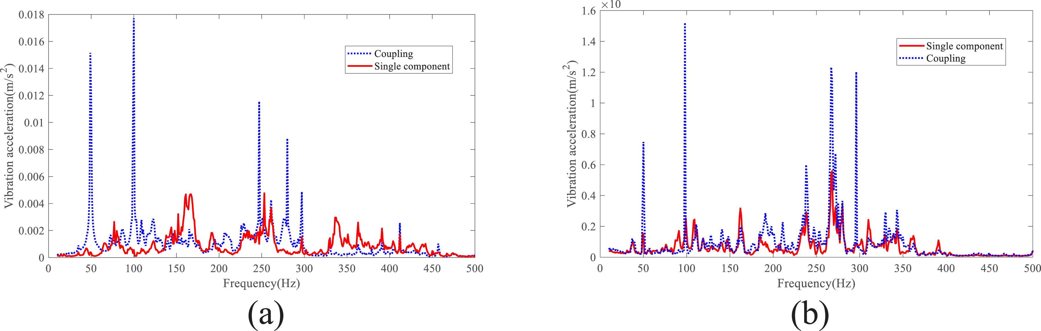

The results simultaneously demonstrate that in pump-valve pipeline systems, vibrations of pump are not solely transmitted through pipe walls and equipment mountings, but can also propagate via fluid flow. The flow-transmitted vibrational loads may induce coupled vibrations with other equipment components, resulting in significant response amplifications at specific frequency bands. Practical measures should be implemented to suppress this phenomenon in engineering.

3.2. Characterizations of FIV during valve closing process

In engineering, the valve is an important component for control and serves as a primary means of regulating pump performance. By adjusting the valve opening, the pump’s operating condition can be modified, altering the pipeline flow rate. With valve closes, pump quickly transitions from stable operating point to the shutdown operating point over short periods of time. The transient flow characteristics differ significantly from steady-state operation, exhibiting strong dynamic coupling effects. After validating the accuracy of the 1D-3D coupled FIV algorithm, this study further investigates the dynamic coupling effect between the valve closure and pump behavior. Pump is modeled in 3D while other components are modeled in 1D. The valve opening is controlled by a controller. The initial opening of the valve is 0.42, and it is completely closed in 1 s time. By pre-calculating the piping system in full 1D, the initial flow rate and lift of pump are 41.2 kg/s and 28.7 m, respectively.

Before simulating the valve closing process, the steady-state coupled flow field calculation is performed at the initial valve opening. The transient coupling simulation then proceeds, using the steady-state results as initial conditions. Convergence is ensured in each time-step before advancing. The total closure time is 1 s, discretized into 1000 steps of 0.001 s each. Figure 10 compares the coupled and 1D simulation results. While both methods yield similar mass flow rates, the lift differs more significantly. The difference in flow rate is reflected in initial moment, which is due to the transient coupling calculation of pump flow rate and lift and other external characteristics of the parameters are pulsating changes. There will be a certain difference compared with steady-state coupling calculation. The lift difference becomes pronounced in the second half of valve closure. Initially, the coupled and 1D results align closely, but as the valve opening decreases, the 3D-coupled lift increases faster than the 1D prediction. This is mainly because the 1D transient calculation for the discrete quasi-steady-state flow-lift curve of the pump is a pseudo-transient calculation. The calculation results can not reflect the pump-valve shutdown process of transient characteristics.

Figure 10.

Comparison of pump mass flow and lift between 1D and 3D calculations: (a) lift and (b) mass flow rate.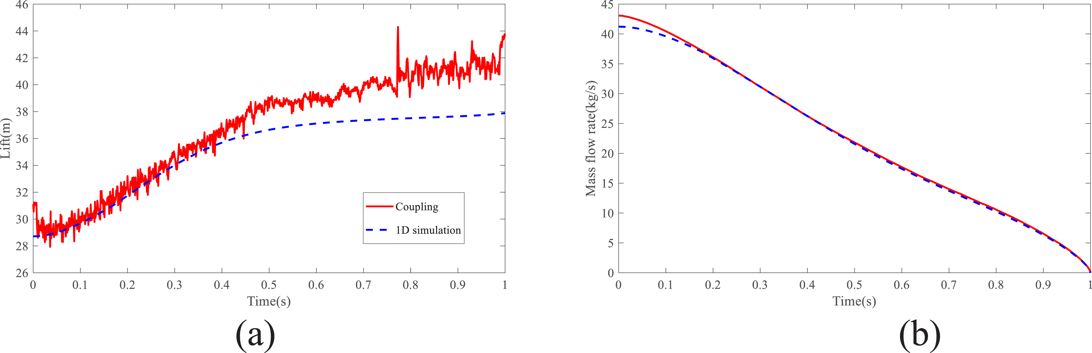

Based on the previous study, influence law for valve closing times upon the transient characteristics of pumps was further investigated. The coupled flow field calculations were carried out for a valve closing time of 0.5 s. The changes in flow rate and lift were compared with those for 1 s in Figure 11. Both the rate of increase in head and the rate of decrease in mass flow increase as the valve closing time decreases. The lift of the pump with a valve-off time of 0.5 s is greater than that with a valve-off time of 1 s, and the flow rate at 0.5 s is smaller than that at 1 s. But the shut-off time will not affect the trend of the head change. For both cases, the head increase speed slows down with the valve opening degree decreases. It should be noted that at 0.5 s, there is a step increase in head, which is not obvious at 1s. This pressure step increase can cause damage to the pump, so it is advisable to reduce the valve closing speed for smoother pump operation.

Figure 11.

Comparison of results with different valve closing time: (a) lift and (b) mass flow rate.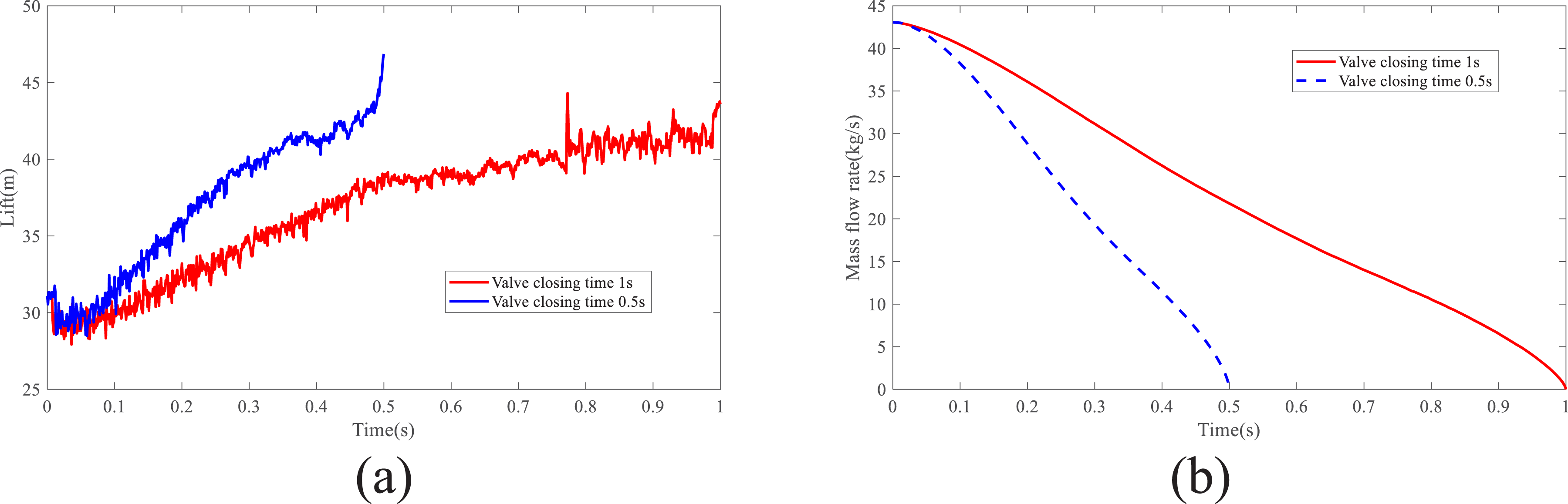

Figure 12 gives the flow head for pump at different valve closing times. At high flow rates, little effect is observed on the external characteristics by the valve closing time. When the flow rate drops below 20 kg/s, the transient characteristics begin to differ. A faster valve closing time is correlated with a higher corresponding head. The transient effect is found to be more pronounced at 0.5 s compared to 1 s. Therefore, in order to avoid the pump head being too high due to transient effects when the valve is closed, the time should be extended as much as possible.

Figure 12.

Comparison of transient characteristics of different valve closing time.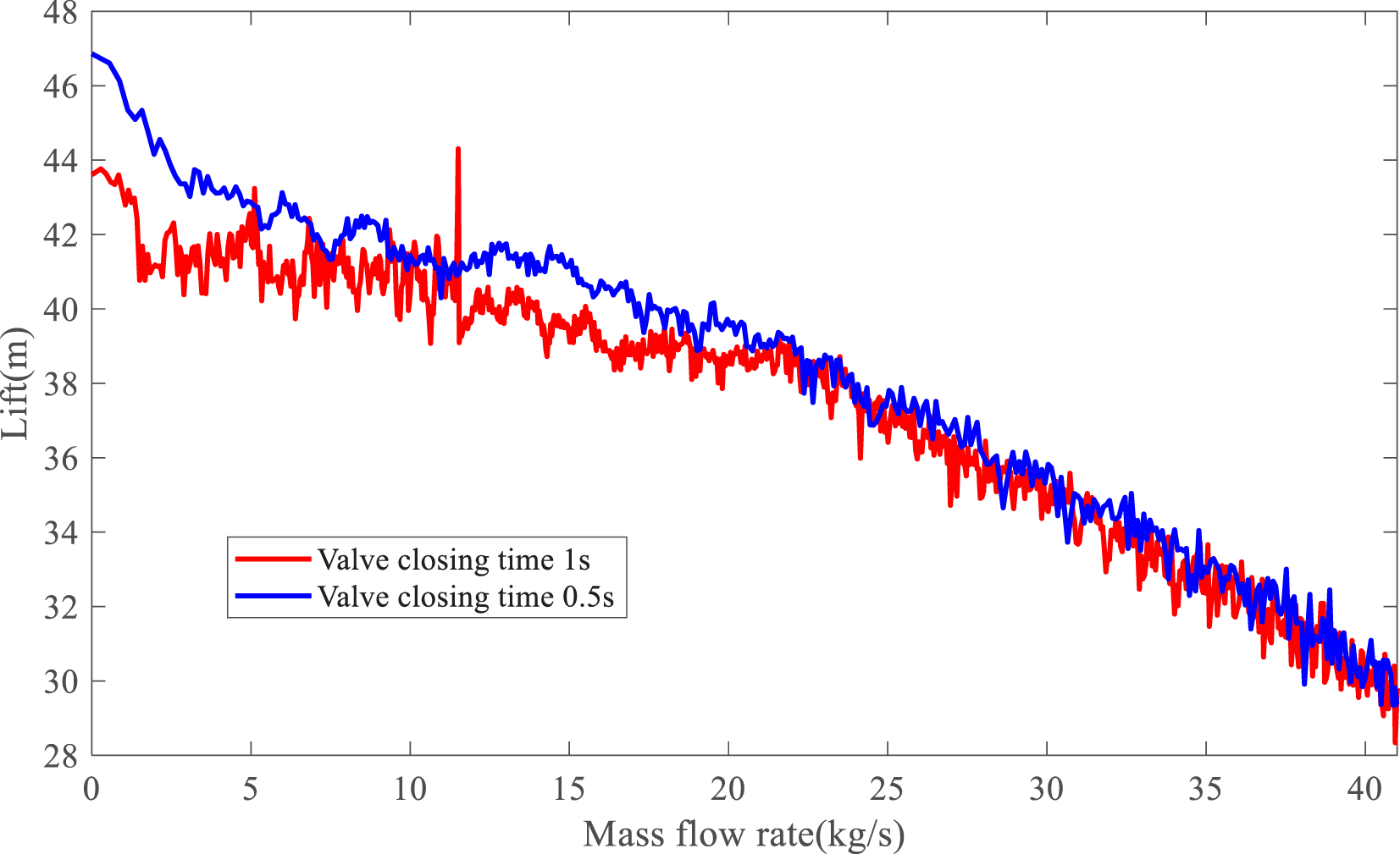

To explore the influence of valve closing mode to transient effect in pumps, the transient characteristics for pumps were analyzed under nonlinear valve shutdown conditions, where the valve was initially closed from 0.42 to 0.3 within the first 0.5 s, followed by a further closure from 0.3 to 0 in the subsequent 0.5 s. This was compared with the flow rate and lift for the same total time, but the shutdown method was linear shutdown, which is displayed on Figure 13. Under nonlinear shutdown conditions, the increase in lift and decrease in flow rate were initially gradual, whereas in the second phase, both changes accelerated significantly. This phenomenon is primarily attributed to the varying valve opening speeds during the initial and final stages of the nonlinear shutdown process. Therefore, to maintain a linear increase in pump head during valve opening, it is recommended to reduce the initial valve opening speed.

Figure 13.

Comparison with different valve closing rule: (a) lift and (b) mass flow rate.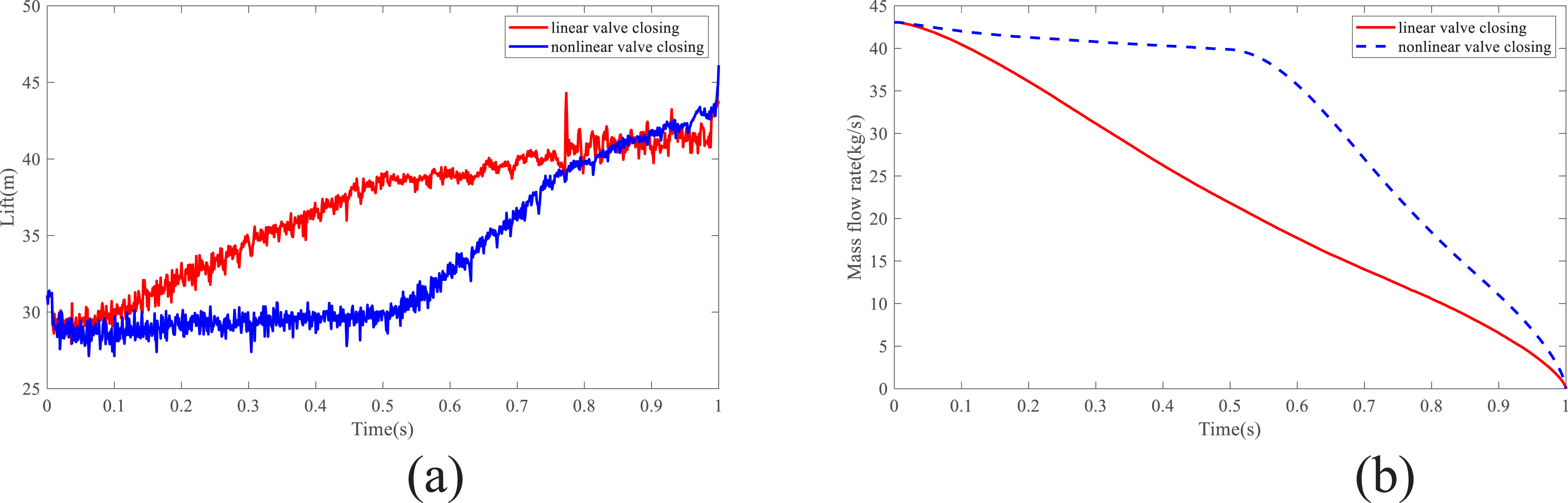

To facilitate a clearer comparison of transient flow and head variations under different valve closure laws, the corresponding flow rate and lift are presented in Figure 14. The valve closure law shows a similar trend with the valve closure time, with negligible effects observed at high flow rates. However, the transient characteristics of the two begin to differ when the flow rate drops below 20 kg/s. A higher head is observed under nonlinear closure conditions at same flow rates. This is mainly because the stronger influence of the latter phase of nonlinear closure on transient behavior. The closure speed in the final stage is significantly higher than that in the initial stage of nonlinear closure. Considering both closure time and closure law, the valve closure process when the pump flow head transient characteristics are mainly reflected in the low-flow segment.

Figure 14.

Comparison of transient characteristics of different valve closing rule.

The transient loads obtained from calculation are applied to the structural model via the interface program. The transient dynamics method is used to analyze FIV performance associated with pump in valve closing process. Considering that pump exhibits initial displacement and velocity before the valve is closed, the time integration effect is disabled during the initialization phase. Static calculations are performed by applying the load of the first time-step at small time intervals. These results are utilized as initial conditions for transient calculations, after which the time integration algorithm is activated for subsequent transient dynamics analysis.

The acceleration at each monitoring point on the pump at the linear valve closing time of 1s is given from Figure 15(a). Vibration response of the pump at each position during the valve shutdown process is the same, with the y-direction acceleration demonstrating significantly higher magnitudes compared to the other two directions. This phenomenon primarily stems from the pump gradually deviates from the rated condition when the valve is closed, the internal flow rate decreases. The speed of fluid in the volute is smaller than that in the impeller. The fluid flowing out of the impeller is constantly hitting the fluid in the volute, causing it to absorb energy, so that the pressure in the volute increases in the circumferential direction. This results in unbalanced radial forces along the radial (x, y) directions. Since the pump features two single volutes arranged 180° apart (Zhou et al., 2023), pressure in semicircle of two volutes is approximately the same. Although deviating from design condition, it reduces the radial force in the x-direction of the pump. The radial force along the y-axis cannot be balanced; therefore, the acceleration along the y-axis will be much greater than the other two directions. With the valve closed, force on the pump in the y-direction gradually increased, the acceleration also increased. By 0.5 s, the internal lift of the pump increases at a slower rate, indicating that the energy exchange rate of fluid inside both the volute and the impeller also slows down. The force in y-direction applied to impeller is also gradually stabilized, so the FIV response is also stabilized. Figure 15(b) shows the comparison of the FIV of pump under different closing times. The response under both closing conditions reaches the maximum value at 0.25 s and 0.5 s, respectively. The closing time does not have much influence on the maximum vibration response, mainly because the flow rate corresponding to the slowdown of the head growth in 0.25 s and 0.5 s is approximately 20 kg/s. At this stage, the radial force exerted on the pump is roughly equal.

Figure 15.

Fluid-induced vibration response of pump: (a) at different positions in valve closing process and (b) with different valve closing times.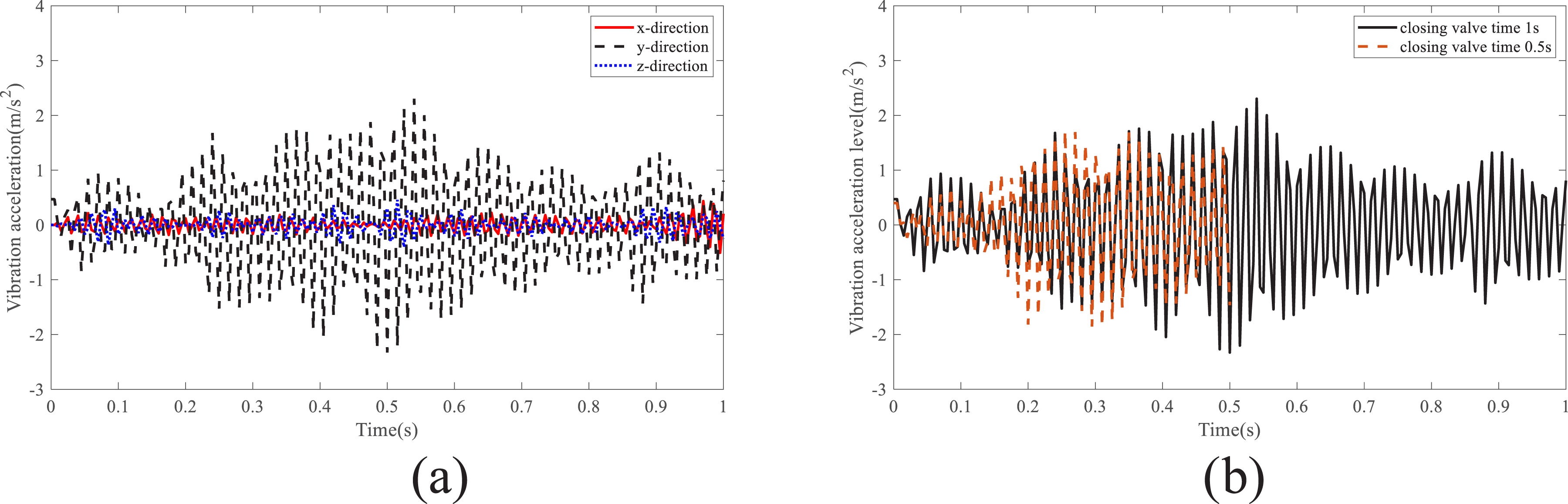

The two valve closing methods in the whole system mentioned above are comparatively difficult to achieve experimentally. However, the simulation of these two phenomena based on the 1D-3D coupled method in this study, effectively fills this research gap, and demonstrates significant engineering application value. In practical engineering applications, excessively rapid valve closure or nonlinear valve closure (characterized by unsteady closing velocity) can markedly amplify equipment vibration, thereby causing damage to the equipment. Such damage is not confined to the valve itself. It can also propagate through the pipeline and the fluid to other equipment, leading to potentially severe consequences for the entire system. Therefore, these two phenomena should be rigorously avoided in engineering.

4. Conclusions

Based on the 1D-3D coupled method, the flow and FIV characteristics of the pump-valve-pipe system are analyzed. A coupled flow field computational model of the piping system is established, and a 1D-3D coupled computation of the whole system is performed. Factors affecting the accuracy and efficiency are investigated. The convergence speed increases as the α increases, but the instability also increases. With the increase in the number of CFD iterations per coupling step, the stability for convergence gradually improves, but the costs also increase. Based on the unidirectional decomposition coupling of the fluid excitation load extraction strategy, the secondary development of the flow field and structure software was conducted. The interface program was developed to realize the following functions: fluid load extraction, interpolation mapping of the fluid load from the flow field mesh to the structural mesh, time-frequency processing of the load, and load application. The FIV models for each component of the entire system were established, respectively. The pulsating pressure on different parts are extracted by coupled flow field calculation. The loads are applied to the finite element model of system by using the secondary development interface program, enabling the analysis of the FIV characteristics of the piping system under multi-source fluid loads. The results show that the spectral curve contains more spectral information and successfully captures the shaft frequency, lobe frequency, and their harmonic frequencies of the pump, whereas the calculation for a single piping component does not reflect the frequency characteristics of the pump source. Accuracy was validated experimentally, and the simulations agreed well with the experimental results. The transient characteristics of pumps under different valve shut-off modes were further investigated. The results show that the effects of different valve shut-off methods on the pump are primarily observed in the low-flow region during the latter half of the operation.

The method used in this paper can analyze the flow field and FIV characteristics of the whole piping system from a system-level perspective with high accuracy, which is of high value in engineering applications. However, several limitations still exist. (1) The coupling efficiency could be further improved; (2) The two-way fluid-structure interaction cannot be considered. These two issues are essentially related to the use of commercial software. During the coupling process, Fluent is primarily invoked through scripts and User-Defined Functions, which lead to a reduction in efficiency. If more flexible open-source software, such as OpenFOAM, or self-compiled codes were employed, the current coupling efficiency could be further enhanced, which represents a primary research objective for future studies. Regarding the second point, the implementation of system-level two-way fluid-structure interaction would require at least three software packages. This limitation similarly depends on the availability of more flexible software codes. Therefore, a 1D-3D coupled method based on independently programmed software is expected to significantly improve the existing approach, representing a critical direction for future advancements.

Footnotes

Declaration of conflicting interests

The author(s) declared no potential conflicts of interest with respect to the research, authorship, and/or publication of this article.

Funding

The author(s) disclosed receipt of the following financial support for the research, authorship, and/or publication of this article: This work was supported by the National Natural Science Foundation of China under Grant nos. 52241101; National Natural Science Foundation of China under Grant nos. 52225109; and National Natural Science Foundation of China under Grant nos. 52271309; and Natural Science Foundation of Heilongjiang Province of China under Grant nos. YQ2022E104.

ORCID iDs

Guoyong Jin

Tiangui Ye

Appendix

References

Adamkowski

Henclik

Lew

, et al. (2010) Experimental and numerical results of the influence of dynamic Poisson effect on transient pipe flow parameters. IOP Conference Series: Earth and Environmental Science.

Ahmadi

Keramat

(2010) Investigation of fluid–structure interaction with various types of junction coupling. Journal of Fluids and Structures 26(7-8): 1123–1141.

Ahmed

Eames

Azarbadegan

, et al. (2022) Acoustics and vibrations in a complex piping network with pump startup-shutdown transients. International Journal of Mechanical Sciences 227: ■■■.

Al-Khomairi

(2003) Use of steady-state pump head-discharge curve for unsteady pipe flow applications. Journal of Hydraulic Engineering 129(12): 1001–1006.

Askarian

Permoon

Shakouri

(2020) Vibration analysis of pipes conveying fluid resting on a fractional Kelvin-Voigt viscoelastic foundation with general boundary conditions. International Journal of Mechanical Sciences 179: ■■■.

Benra

(2006) Numerical and experimental investigation on the flow induced Oscillations of a single-blade pump impeller. Journal of Fluids Engineering 128(4): 783–793.

Chen

(2012) Noise and vibration in complex hydraulic tubing systems. In: Gan

Y. X.

(ed). Continuum Mechanics - Progress in Fundamentals and Engineering Applications. IntechOpen. Available at: https://doi.org/10.5772/39178

Ding

(2023) Vibration control of fluid-conveying pipes: a state-of-the-art review. Applied Mathematics and Mechanics 44(9): 1423–1456.

Domnick

Brillert

(2019) Flow-induced steam valve vibrations-A literature review of excitation mechanisms, preventive measures, and design improvements. Journal of Engineering for Gas Turbines & Power 141(5): 051009.

10.

Durant

Robert

Filippi

, et al. (2000) Vibroacoustic response of a thin cylindrical shell excited by a turbulent internal flow: comparison between numerical prediction and experimentation. Journal of Sound and Vibration 229(5): 1115–1155.

11.

Fei

(2013) Study on Fluid-Solid Coupling Mechanism and Unsteady Flow Intensity of Transient Hydraulic Excitation in Centrifugal Pump. Jiangsu university.

12.

Gao

Zhang

Liu

, et al. (2020) Vibration analysis of aero parallel-pipeline systems based on a novel reduced order modeling method. Journal of Mechanical Science and Technology 34(8): 3137–3146.

13.

Gao

Zhang

, et al. (2021) Vibration analysis and control technologies of hydraulic pipeline system in aircraft: a review. Chinese Journal of Aeronautics 34(4): 83–114.

14.

Guo

(2017) Analysis of Unsteady Flow and Vibration Characteristics of Low Specific Speed Centrifugal Pump Based on Two-Way Fluid-Solid Coupling. Zhejiang Sci-tech university.

15.

Guo

Zhou

Chen

, et al. (2023) Flow-induced vibration analysis in a pump-turbine runner under transient operating conditions. Engineering Applications of Computational Fluid Mechanics 17(1): ■■■.

16.

Heinsbroek

(1997) Fluid-structure interaction in non-rigid pipeline systems. Nuclear Engineering and Design 172(1-2): 123–135.

17.

Jiang

Yoshimura

Imai

, et al. (2007) Quantitative evaluation of flow-induced structural vibration and noise in turbomachinery by full-scale weakly coupled simulation. Journal of Fluids and Structures 23(4): 531–544.

18.

Kong

Noroozi

Rahman

AGA

, et al. (2014) Non-destructive testing and assessment of dynamic incompatibility between third-party piping and drain valve systems: an industrial case study. Nondestructive Testing and Evaluation 29(2): 154–163.

19.

(2011) Study on Vibration Noise and Characteristics of Pipeline System Considering Fluid-Solid Coupling. Harbin ENgineering University.

20.

Tang

(2007) Experiment and simulation of non-contact flow measurement based on vibration principle. Experimental Considerations Fluid Mechanics 21(1): 5.

21.

Deng

Jiang

(2019) Dynamic response and vibration suppression of a cantilevered pipe conveying fluid under periodic excitation. Journal of Vibration and Control 25(11): 1695–1705.

22.

(2015) Fluid-solid Coupling Dynamics Calculation and Characteristic Analysis of Pipeline System. Harbin Engineering University.

23.

Bai

Wang

(2023) Experiments and numerical analysis of the dynamic flow characteristics of a pump-pipeline system with entrapped air during start-up. Engineering Applications of Computational Fluid Mechanics 17(1): ■■■.

24.

Liu

(2013) One-dimensional and Three-Dimensional Transient Coupling Simulation of Centrifugal Pump System Characteristics. Zhejiang University.

25.

Ljubijankic

Nytsch-Geusen

Rädler

, et al. (2013) Numerical coupling of Modelica and CFD for building energy supply systems. In: The 8th International Modelica Conference. Technical Univeristy, Dresden, Germany.

26.

Misra

Behdinan

Cleghorn

(2002) Self-excited vibration of a control valve due to fluid-structure interaction. Journal of Fluids and Structures 16(5): 649–665.

27.

Papukchiev

Lerchl

(2012) Extension and application of the coupled 1D-3D thermal-hydraulic code ATHLET-ANSYS CFX for the simulation of liquid metal coolant flows in advanced reactor concepts. In: International Conference on Nuclear Engineering & the Asme Power Conference. ■■■.

28.

Pittard

Evans

Maynes

, et al. (2004) Experimental and numerical investigation of turbulent flow induced pipe vibration in fully developed flow. Review of Scientific Instruments 75(7): 2393–2401.

29.

Qing

Jinghui

Yushan

, et al. (2006) Experimental studies of orifice-induced wall pressure fluctuations and pipe vibration. International Journal of Pressure Vessels and Piping 83(7): 505–511.

30.

Ryu

Kim

, et al. (2004) Vibration and dynamic stability of pipes conveying fluid on elastic foundations. KSME International Journal 18(12): 2148–2157.

31.

Stangl

Irschik

(2005) Vibrations of pipes with internal flow and rigid body degrees of freedom. Pamm 5(1): 137–138.

32.

Tijsseling

(2004) Exact solution of linear hyperbolic four-equation system in axial liquid-pipe vibration. Journal of Fluids and Structures 18(2): 179–196.

33.

Tijsseling

Vardy

(2004) Time scales and FSI in unsteady liquid-filled pipe flow. Technische Universiteitndhoven.

34.

Viel

Marcer

Audiffren

, et al. (2010) Coupling 1D system AMESim and 3D CFD EOLE models for diesel injection simulation. In: ILASS – Europe 2010, 23rd Annual Conference on Liquid Atomization and Spray System. ■■■.

35.

Wang

Bai

Sheng

(2019) Influence of two-way fluid-solid coupling on internal and external characteristics of screw centrifugal pump. General Machinery 1(3): 5.

36.

Whatham

(1987) Analysis of pipe bends with symmetrical noncircular cross sections. Journal of Applied Mechanics 54(3): 604–610.

37.

Liu

, et al. (2012) The research of 1D / 3D coupling simulation on pump and pipe system. IOP Conference Series: Earth and Environmental Science 15(5): 052032.

38.

Xue

Tian

Cheng

, et al. (2024) Mechanism analysis of the abnormal head-cover vibration of an ultra-high-head pump-turbine operating in pump mode by CFD and FEM. Engineering Applications of Computational Fluid Mechanics 18(1): ■■■.

39.

Yan

(2011) Development of a Coupled CFD---system-code capability (with a modified porous media model) and its applications to simulate current and next generation reactors. Dissertations & Theses - Gradworks.

40.

Yang

(2015) Study on transient characteristics of pumping system based on MOC-CFD coupling method. Zhejiang University.

41.

Yonezawa

Ogawa

Ogi

, et al. (2012) Flow-induced vibration of a steam control valve. Journal of Fluids and Structures 35(Complete): 76–88.

42.

Zeid

Shouman

(2019) Flow-induced vibration on the control valve with a different concave plug shape using FSI simulation. Shock and Vibration 2019: 1–14.

43.

Zhang

Tijsseling

Vardy

(1999) Fsi analysis of liquid-filled pipes. Journal of Sound and Vibration 224(1): 69–99.

44.

Zhang

Ouyang

(2015) Structural vibration and fluid-borne noise induced by turbulent flow through a 90° piping elbow with/without a guide vane. International Journal of Pressure Vessels and Piping 125: 66–77.

45.

Zhang

You

, et al. (2020) CFD-rotordynamics sequential coupling simulation approach for the flow-induced vibration of rotor system in centrifugal pump. Applied Sciences 10(3): 1186.

46.

Zhao

Chai

(2024) Simulation study on the flow-induced vibration and noise in marine centrifugal pumps. Journal of Vibration and Control 30(11-12): 2549–2567.

47.

Zhao

Sun

(2018) Flow-induced vibration of curved pipe conveying fluid by a new transfer matrix method. Engineering Applications of Computational Fluid Mechanics 12(1): 780–790.

48.

Zhou

Jin

, et al. (2023) Fluid-induced vibration analysis of centrifugal pump including rotor system based on Computational Fluid Dynamics and Computational Structural Dynamics coupling approach. Ocean Engineering 288: 115993.