
Abstract
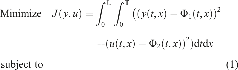
This paper introduces a novel pseudo-spectral (PS) method tailored for the numerical solution of optimal control problems (OCPs) governed by partial differential equations (PDEs). The proposed technique leverages two-dimensional interpolating polynomials constructed on shifted Legendre-Gauss-Lobatto nodes to approximate the state and control variables. This spectral discretization transforms the original infinite-dimensional control problem into a finite-dimensional nonlinear programming (NLP) formulation, enabling efficient numerical treatment. To solve the resulting NLP, we derive the Karush-Kuhn-Tucker (KKT) optimality conditions in full detail, leading to a system of algebraic equations that encapsulate the necessary conditions for optimality. The Levenberg-Marquardt algorithm, known for its robustness in solving nonlinear algebraic systems, is then employed to solve this system iteratively, yielding an accurate approximation of the optimal solution. The effectiveness and reliability of the proposed method are demonstrated through a series of benchmark numerical examples involving PDE-constrained OCPs. Comparative analyses reveal that our approach not only achieves superior accuracy and computational efficiency compared to existing methods but also offers notable advantages in terms of implementation simplicity and scalability. These features make it a compelling alternative for tackling complex OCPs in various scientific and engineering domains.
Keywords
Introduction
Optimal control problems (OCPs) governed by partial differential equations (PDEs) arise in diverse applications such as mechanics, economics, robotics, and aeronautics. Broadly, there are two main classes of methods for solving OCPs: direct methods, which follow a discretize-then-optimize approach, and indirect methods, which follow an optimize-then-discretize philosophy. Direct methods rely on discretization and parameterization, ultimately transforming the problem into a nonlinear programming (NLP) formulation. This class encompasses a wide range of techniques, including quasi-linearization, steepest descent, quasi-Newton approximations, spectral and pseudo-spectral (PS) methods, algorithmic differentiation, finite difference methods (FDMs), finite element methods (FEMs), measure-theoretic approaches, linearization techniques, control parameterization, time-scaling transformations (Huang et al., 2025; Noori Skandari and Tohidi, 2011), and reproducing kernel algorithms (Abu, 2018; Abu and Shawagfeh, 2021). Among these, direct collocation methods are arguably the most powerful for solving general OCPs. In direct collocation, both state and control variables are approximated using specified functional forms (Noori Skandari et al., 2016). Some direct numerical methods, such as FDMs and FEMs, require the construction of computational meshes and typically operate locally. In contrast, spectral methods, being globally defined and continuous, do not require mesh construction (Samadi et al., 2024). Indirect methods, on the other hand, are grounded in the Pontryagin Minimum (or Maximum) Principle (PMP) and the Hamilton–Jacobi–Bellman (HJB) equations. These approaches yield necessary optimality conditions that often lead to boundary or initial value problems. Such problems can be effectively addressed using collocation techniques, as well as spectral and PS methods (Kang et al., 2008; Noori Skandari et al., 2016). The divergence in philosophy between direct and indirect methods has led to a methodological dichotomy within the optimal control community. Researchers favoring indirect methods tend to focus on differential equation theory, while those employing direct methods are more concerned with optimization algorithms (Biegler et al., 2003). Direct methods are particularly valued for their high convergence rates and the availability of efficient NLP solvers. Interestingly, the covector mapping principle (CMP) has demonstrated that when PS collocation is employed, the distinction between direct and indirect methods essentially disappears (Bertolazzi and Biral, 2023).
A comprehensive summary of gradient-based methods for solving OCPs was provided in Polak (1973, 553–584). The historical development of OC from 1950 to 1985, including an elegant overview of the calculus of variations dating back to the 1600s, is documented in Bryson (1996, 26–33). In Von Stryk and Bulirsch (1992, 357–373), a concise list of commonly used methods developed prior to the 1990s is presented, emphasizing the effectiveness of combining indirect and direct approaches, referred to as hybrid methods. A brief description of techniques for converting continuous-time OCPs into parameter optimization problems is given in Hull (1997, 57–60). Numerical solutions of OCPs governed by PDEs have been explored using various advanced techniques, including: Legendre polynomials and the Ritz method (Mamehrashi and Yousefi, 2017), Generalized Lagrangian Jacobi-Gauss-Radau (GLJGR) collocation method (Latifi et al., 2020), Shifted Gegenbauer polynomial (ShGP) method (Soufivand et al., 2023), Fractional-order Bernstein polynomials (BPs) method (Ketabdari et al., 2021), and Discrete Krawtchouk polynomials (DKPs) method (Dehestani et al., 2025). Further, Nemati and Yousefi (2017, 1079–1097) studied OCPs using a hybrid Ritz method combined with a fractional operational matrix based on Legendre polynomials. Their approach transforms the OCP into a system of algebraic equations. Additionally, Nemati (2018, 2632–2645) proposed a spectral method using Bernstein polynomials and operational matrices to solve OCPs numerically. Finite element methods (FEMs) were employed in Fuica and Jork (2025), while finite difference methods (FDMs) were used in Zoccolan et al. (2025, 237–260) to solve OCPs under PDE constraints. In Mohammadizadeh et al. (2019, 77–102), an indirect method based on the Chebyshev PS (CPS) technique was proposed for solving OCPs governed by Burgers’ equation. The method first reduces the original problem to a system of PDEs with boundary conditions using optimality principles, then approximates control and state functions via interpolating polynomials. Akkouche et al. (2014, 622–631) applied the variational iteration (VI) method, an indirect approach, to solve a quadratic OCP governed by linear PDEs. The method derives necessary conditions using PMP, leading to the Hamilton–Pontryagin equations, which form a multi-point boundary value problem. In Sabeh et al. (2016, 3350–3360) a computational technique based on the Legendre PS (LPS) method was used to solve a distributed OCP for Burgers’ equation. The LPS method transforms the PDE-constrained OCP into a classical OCP governed by ordinary differential equations, which can be solved using either direct or indirect methods. The resulting OCP is then tackled via an indirect method by deriving and numerically solving the first-order optimality conditions.
An alternative classification of numerical methods for solving OCPs governed by PDEs distinguishes between continuous methods, such as collocation techniques (Huang and Peng, 2024; Jiang and Gao, 2024), and discrete methods, including finite difference, Runge-Kutta, and multi-step schemes (Doehring et al., 2024; Erfanifar and Hajarian, 2024). Although continuous methods can produce discrete approximations at selected points, many discrete methods lack the ability to generate globally continuous approximations. This limitation is particularly evident in extrapolation and Runge-Kutta methods, which are less effective for problems requiring smooth, globally differentiable solutions. For such problems, spectral methods, a specialized subclass of collocation techniques, offer a compelling solution. These methods are designed to produce globally smooth approximations using algebraic polynomials. In particular, PS methods (Pirouzeh et al., 2024; Samadi et al., 2024), a refined form of spectral collocation, have proven highly effective for PDE-constrained OCPs. PS methods enforce the differential equations at strategically chosen collocation points within a finite domain, while ensuring that the polynomial approximations match the exact solution at boundary and initial nodes. This approach guarantees that the resulting approximations are not only accurate but also globally continuously differentiable, a critical property for precise control of dynamic systems and physical phenomena. It should be noted that the significance of spectral and PS methods has recently been acknowledged by some researchers in solving other optimal control problems, including delay and fractional problems (Marzban, 2021; Marzban and Hoseini, 2016; Marzban and Manochehri Naeini, 2026; Marzban and Nezami, 2022; Tabrizidooz et al., 2017).
OCPs governed by PDEs are becoming increasingly prevalent in applied sciences, introducing substantial analytical and computational challenges. Addressing these challenges requires the development of novel mathematical models and advanced numerical techniques, particularly PS methods, which have shown great promise in handling complex, high-dimensional systems. This need is especially pressing for problems involving nonlinear PDE systems, which are directly relevant to practical applications in engineering, physics, and biology. A considerable body of research has focused on OCPs involving semi-linear parabolic equations, a fundamental class in PDE theory. These problems often rely on first-order necessary optimality conditions, typically derived using the PMP (Raymond and Zidani, 1998). In addition, several studies have investigated Karush–Kuhn–Tucker (KKT) conditions and even second-order sufficient conditions to enhance solution robustness and theoretical guarantees (Casas et al., 2008). Despite these advances, existing numerical methods for solving such problems frequently encounter limitations in terms of computational cost and convergence reliability, particularly when applied to highly nonlinear PDEs. The complexity of these systems also complicates error analysis, as thoroughly reviewed in Leugering et al. (2012), Tröltzsch (2010), further emphasizing the need for accurate and efficient algorithms. Moreover, OCPs involving wave-type PDE solutions present additional challenges. Examples include the control of spiral waves (Borzi and Griesse, 2006), and wave propagation in cardiac models (investigated by Kunisch and Wagner, 2013). These problems are computationally demanding and often suffer from convergence issues when tackled with iterative optimization techniques. Such limitations underscore the urgency of developing robust, scalable, and high-fidelity numerical methods tailored to these complex control scenarios (Casas and Yong, 2023; Mowlavi and Nabi, 2023).
To solve OCPs governed by PDEs using indirect methods, one must first derive the necessary optimality conditions. However, these conditions are typically available only for problems involving specific PDEs, such as the Burgers’ equation addressed Mohammadizadeh et al. (2019, 77–102). In general, deriving such conditions is analytically intractable and impractical for broader classes of nonlinear PDEs. Consequently, many researchers have turned to direct methods for solving OCPs involving nonlinear PDEs. These approaches begin by discretizing the original problem into a nonlinear programming (NLP) formulation using techniques such as Runge-Kutta discretization. While effective in principle, these methods often require a large number of discretization points, leading to increased computational complexity. Moreover, the resulting NLP problems typically lack closed-form solutions. These challenges stem from two primary sources: (I) Inefficient discretization techniques, which fail to accurately capture the dynamics of the original OCP. (II) Weak optimization algorithms, which struggle to solve the resulting NLP problems effectively. In contrast, direct methods that utilize the KKT conditions offer a more tractable framework for solving NLP problems. To overcome the aforementioned difficulties, we propose a three-step approach for solving OCPs governed by nonlinear PDEs: Step 1: Discretize the problem using a high-accuracy method such as the Legendre–Gauss–Lobatto (LGL)-PS method. Step 2: Formulate the KKT necessary optimality conditions, including detailed gradient and derivative matrices. Step 3: Solve the resulting algebraic system using a robust numerical solver, such as the Levenberg-Marquardt algorithm, to approximate the optimal solution. This process yields highly accurate approximations and can lead to near-explicit solutions. Among various PS techniques, the LGL-PS method stands out for its superior accuracy in solving continuous-time problems involving both ODEs and PDEs (Hairer and Wanner, 1996; Ogundare, 2009; Wright, 1964). Numerical experiments demonstrate that the LGL-PS method outperforms other approaches, including Legendre PS (LPS), Chebyshev PS (CPS), and variational iteration (VI) methods, in terms of both computational efficiency and solution accuracy (Akkouche et al., 2014; Mohammadizadeh et al., 2019; Sabeh et al., 2016). In the present work, we apply the LGL-PS method to an OCP governed by a general class of second-order nonlinear smooth PDEs. The full formulation of the KKT conditions, including gradient and Jacobian matrices, is provided to support reproducibility and further analysis.
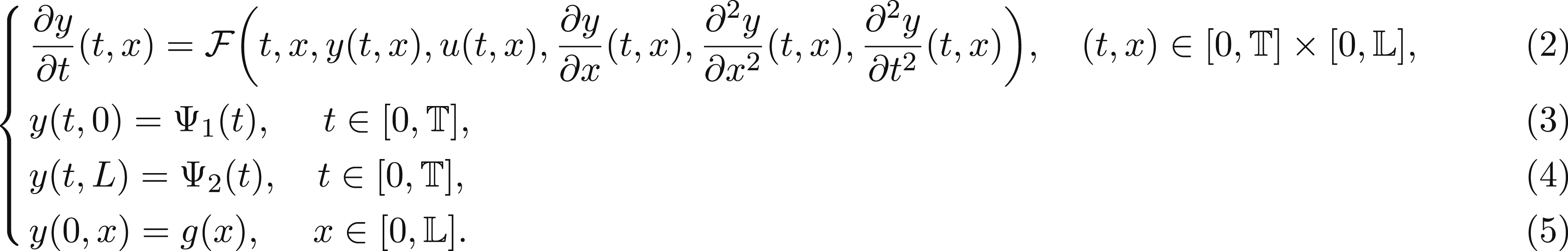
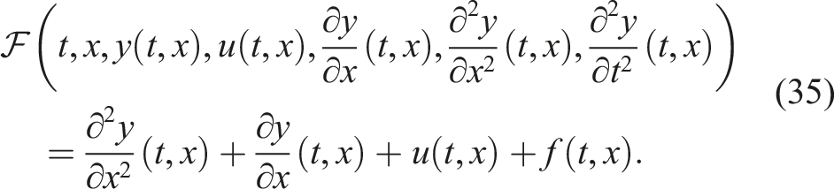
We centralize on the following form of OCPs under PDEs
Here,
This article is structured as follows: In LGL-PS method to approximate the solution section, we implement the LGL-PS method for problem (1)-(5) and gain an NLP problem. In optimality conditions for gained NLP problem section, by writing the KKT optimality conditions for the NLP problem, we arrive at a system of algebraic equations and solve this algebraic system using the Levenberg–Marquardt method. In Numerical examples section, we present some test problems to show the superiority and effectiveness of method to solve OCPs under PDEs.
LGL-PS method to approximate the solutions
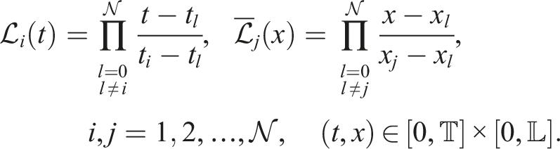
In this paper, we present an approach for numerical solving problem (1)-(5). Suppose


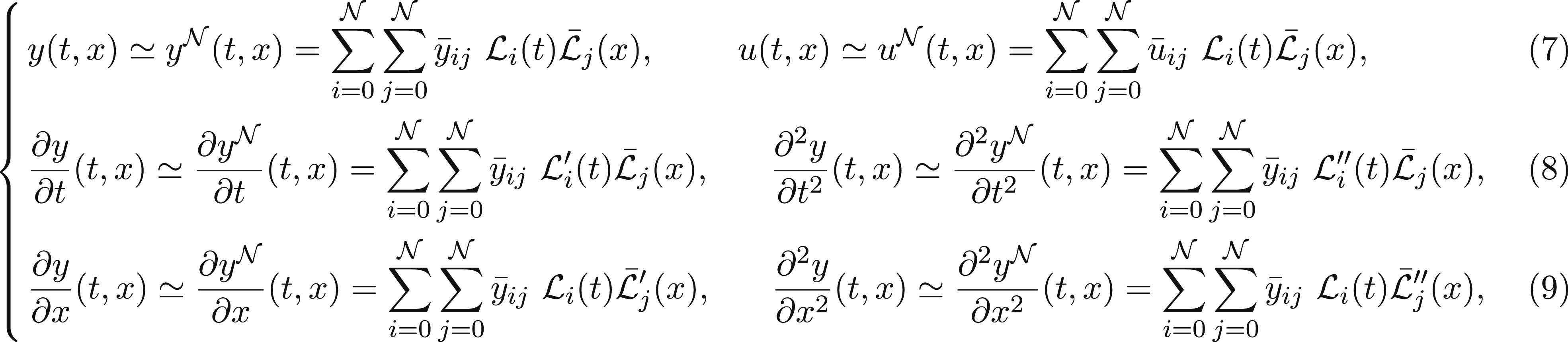 where
where
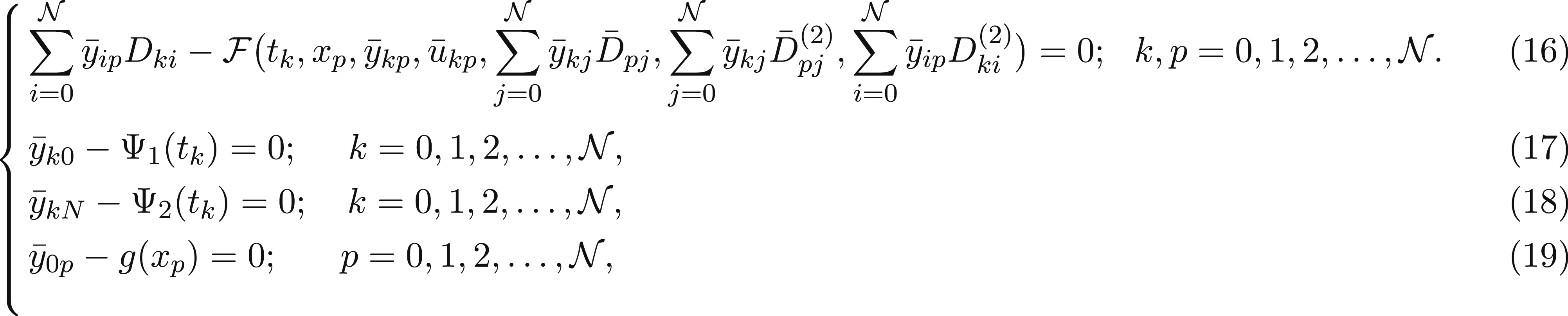
Now, we can discretize the approximations (7)–(9) at the collocation points
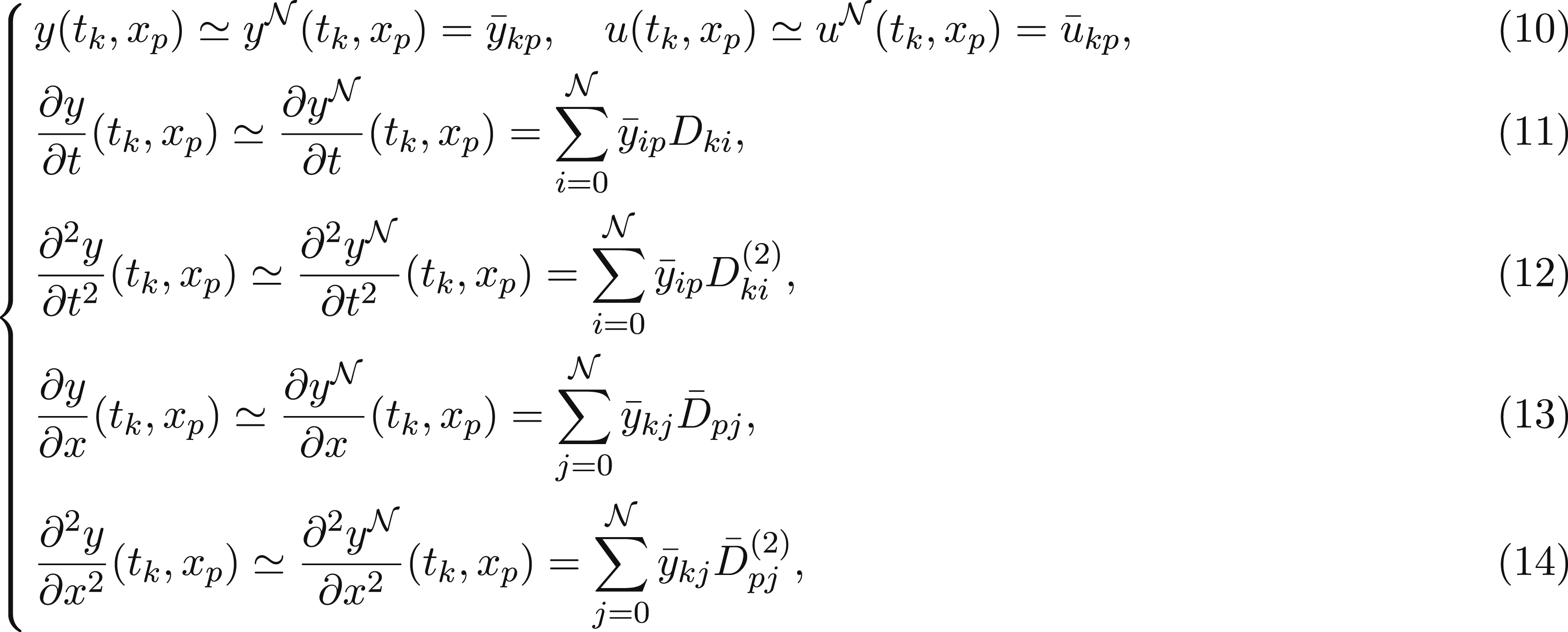 where D = (D
ij
),
where D = (D
ij
),
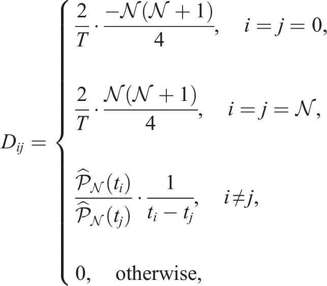
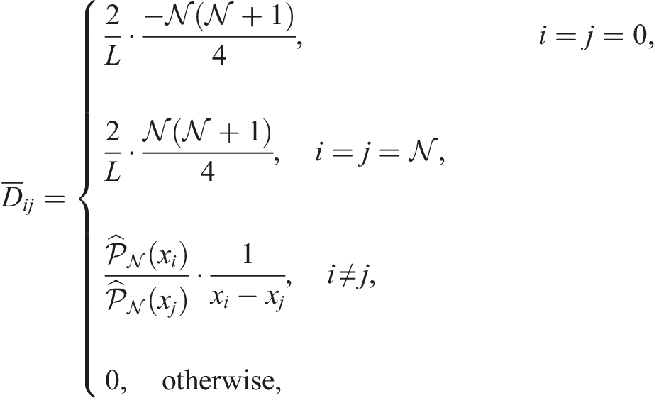
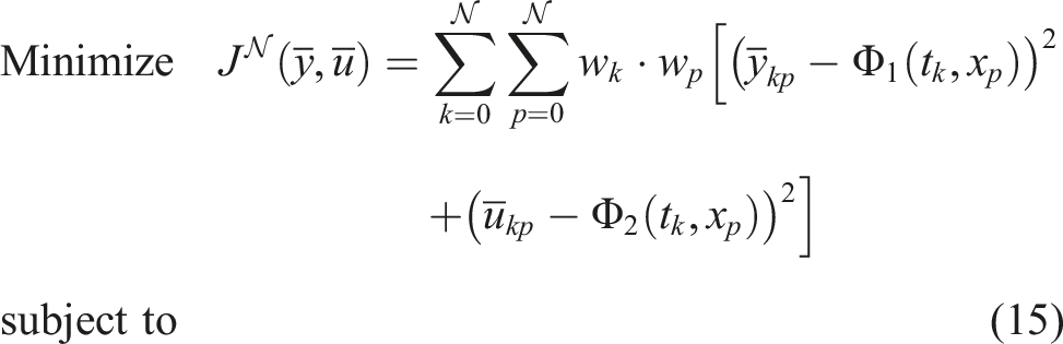
The OCP (1)-(5) can be expressed as follows through discretization according to the aforementioned procedure as mentioned above which is an NLP problem
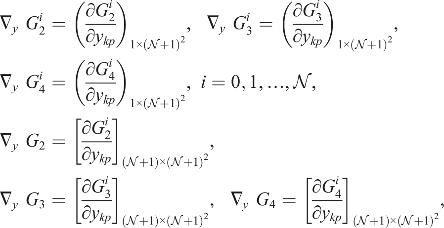
Optimality conditions for gained NLP problem
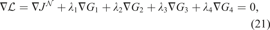
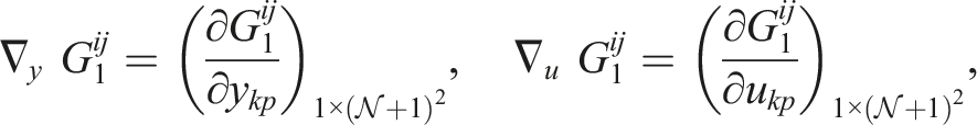
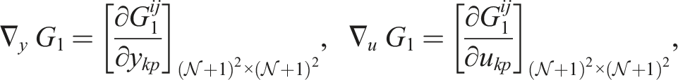
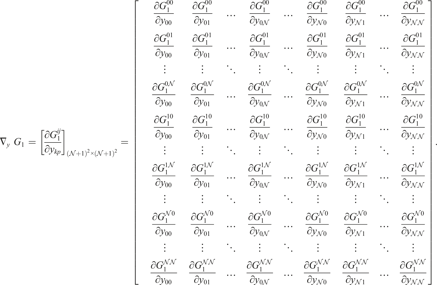
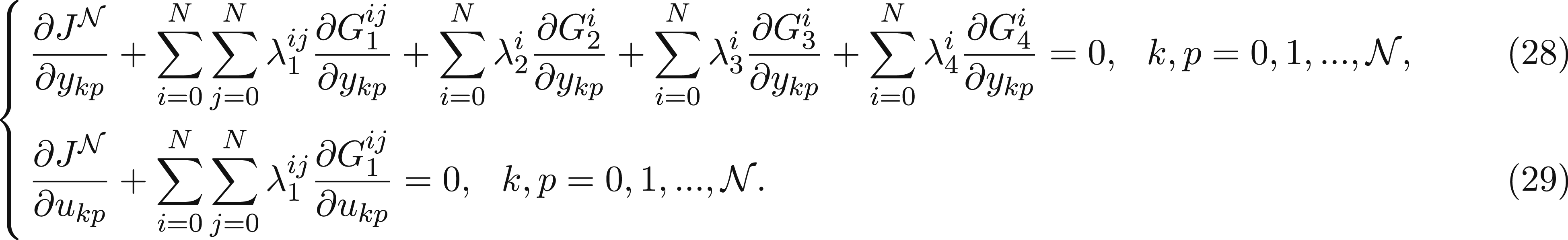
We point out that most of direct methods for solving NLP problems cannot be led to an explicit and accurate solution. So, it is essential that we apply the optimality conditions, that is, KKT conditions. To achieve the KKT conditions, we first denote the constraints (16)-(19) by

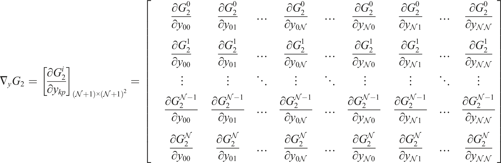
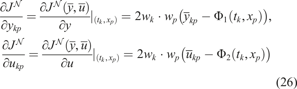
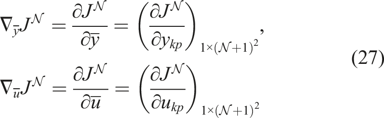
The necessary condition for optimality is

Considering that constraints G1, G2, and G3 do not involve variable u kp , the above system of equations becomes:

We denote the constraints at the collocation points (t
i
, x
j
) as
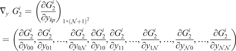
We can write for more explanation
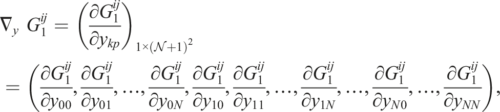
Other cases can be raised in the same way. Moreover, for constraints G2, G3, and G4, the number of each of them has equal to
We can write for more explanation
Other cases can be raised in the same way. Now, regarding the objective functional, we have
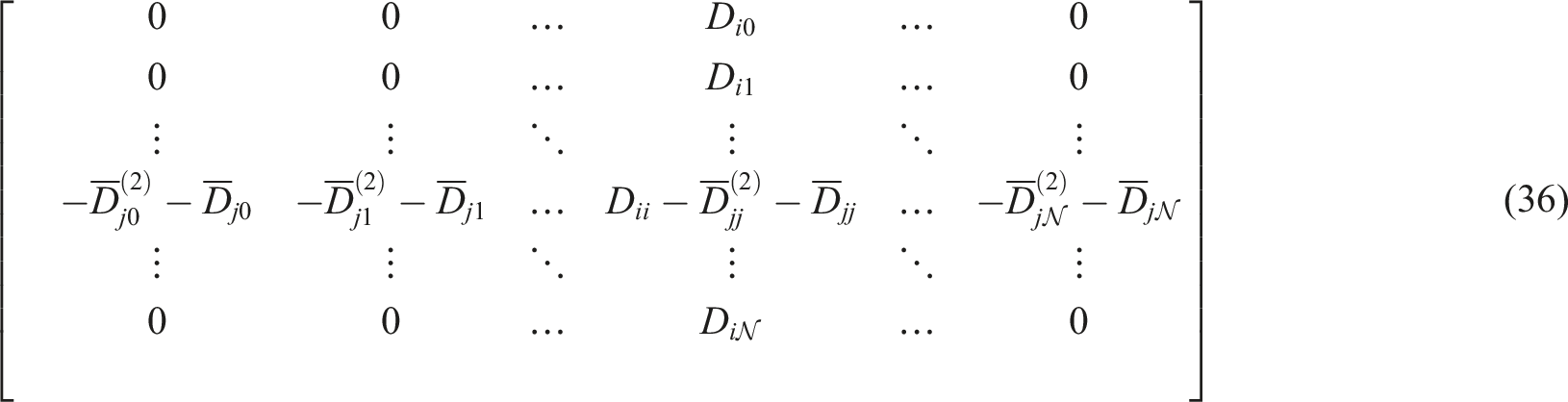
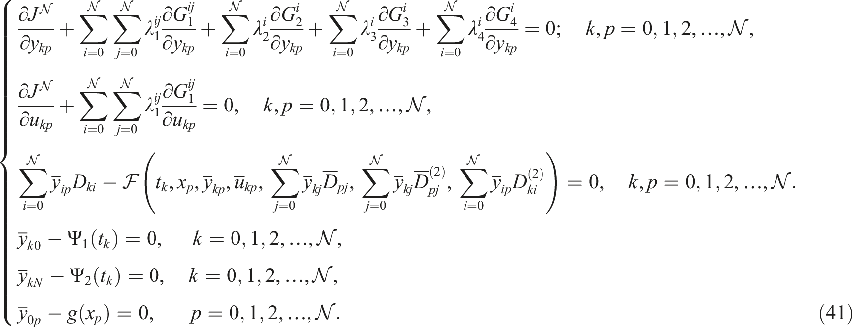
Consequently, the system of equations (15)–(19) is rewritten as follows
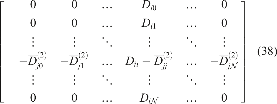
To this system of equations, the following results can be obtained: (A) According to the relationship of (16), we have
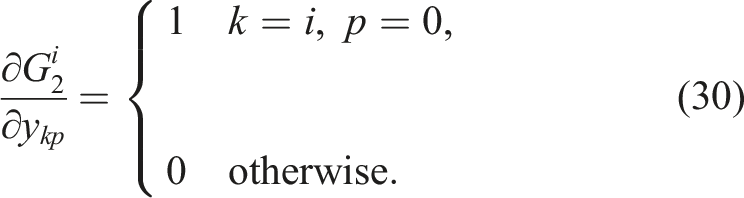
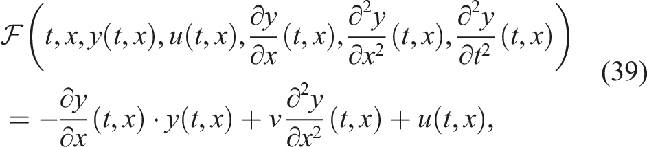
That is, by changing (k, p), the result becomes a vector, where all of its elements except for element (k = i, p = 0), it means the (B) According to (17), we have
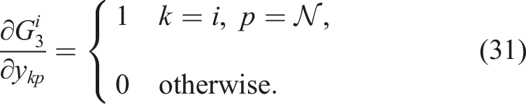
By changing (k, p), the result becomes a vector, where all of its elements except for element (k = i, p = N), it means the (C) As per (18), we have
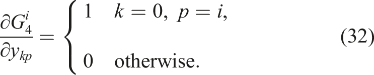
Varying (k, p) results in a vector, where only the element (k = 0, p = i), it means the i − th component of this vector, is non-zero. (D) To solve the system of gradient equations (28) and (29), we need
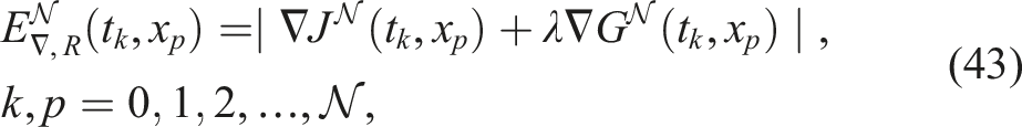
In (15), we have
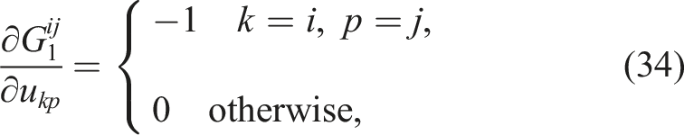
Varying (k, p) results in a vector where only the element (k = i, p = j), it means the
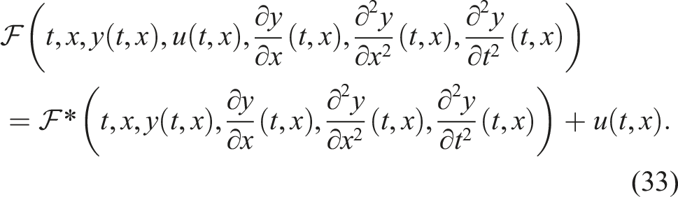
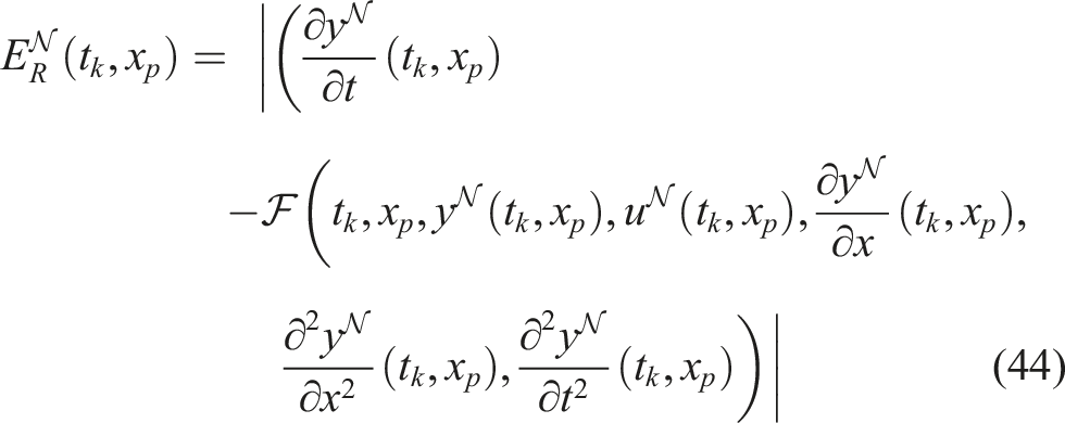
Below, we present equation (15) for the following special OCPs: (I) OCPs under linear equation: we consider
Now, for convenience, we rewrite vector (II) OCPs under diffusion equation: We consider
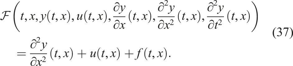
Thus, we have formulated an OCP involving the diffusion equation. We will examine the matrix (III) OCPs under Burgers’ equation: we consider
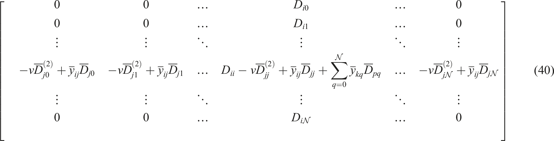
By attention to above calculate matrices and vectors, we achieve the following system of algebraic equations
To determine the number of equations, we first analyze the gradient equations (28) and (29), considering that there are
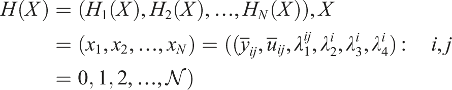
The Levenberg–Marquardt algorithm effectively tackles systems of nonlinear algebraic equations. While often associated with curve fitting, it extends well to solving such nonlinear systems. By modifying the Gauss–Newton method, it addresses challenges posed by ill-conditioned problems or poor initial guesses, using a damping parameter to balance between the Gauss–Newton method (for rapid convergence near the solution) and gradient descent (for stability far from the solution). For clarification, consider the system H(X) = 0, defined as:
The algorithm begins with an initial guess X(0) for the vector X. The Jacobian matrix J(X), containing partial derivatives
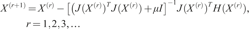
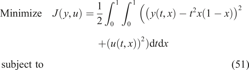
Here, μ is the damping parameter, dynamically adjusted at each iteration and I is the identity matrix. This approach combines the fast convergence of the Gauss–Newton method with the stability of gradient descent. Convergence is assessed by the norm of the residual vector H(X(r+1)), and the algorithm stops when this norm falls below a predefined threshold, indicating a solution.
Levenberg–Marquardt is a popular alternative to the Gauss–Newton method of finding the minimum of the function that is a sum of squares of nonlinear functions. This method is a fundamental regularization technique for the Newton method applied to nonlinear equations, possibly constrained, and possibly with singular or even nonisolated solutions. Levenberg–Marquardt method is the most typical algorithm for solving nonlinear algebraic equations. They sequentially solve subproblems represented as squared residual of the Newton equations with the L2 regularization to determine the search direction. Although this method is generally used to solve non-square devices, extensions have recently been added to it to solve square devices (Fischer et al., 2024; Han and Rui, 2024).
In next section, we solve three test problems to show the efficiency of suggested approach compared with others.
Numerical examples
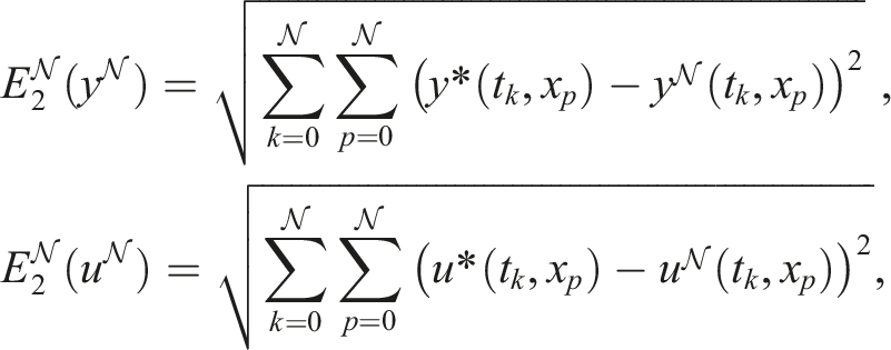
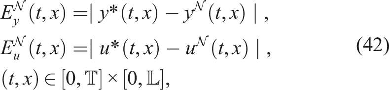
In this section, we solve three OCPs involving PDEs using the proposed method and demonstrate its effectiveness. Referring to the definitions of the 2-norm ‖ ⋅‖2, we will utilize the following relationships to check the convergence of approximate solutions
Finally, we summarize the solution process in in the following algorithm: (1) Select (2) Discretize and obtain the corresponding NLP system according to (15)–(19), (3) Calculate the gradients of the functions in question according to (28) and (29), (4) Solve the algebraic system obtained from the previous steps, which is according to (41), using the Levenberg–Marquardt method, (5) Obtain approximate solutions
Furthermore, it is worth mentioning that the method proposed in this article was implemented and executed using MATLAB software (version 2013) on a personal computer equipped with 6 GB of RAM and an Intel Core i3 processor. The approximate solutions were obtained in less than 10 minutes, which is considered reasonable given the complexity and computational demands of the problems addressed.
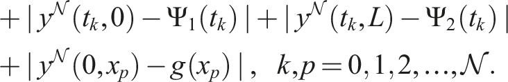
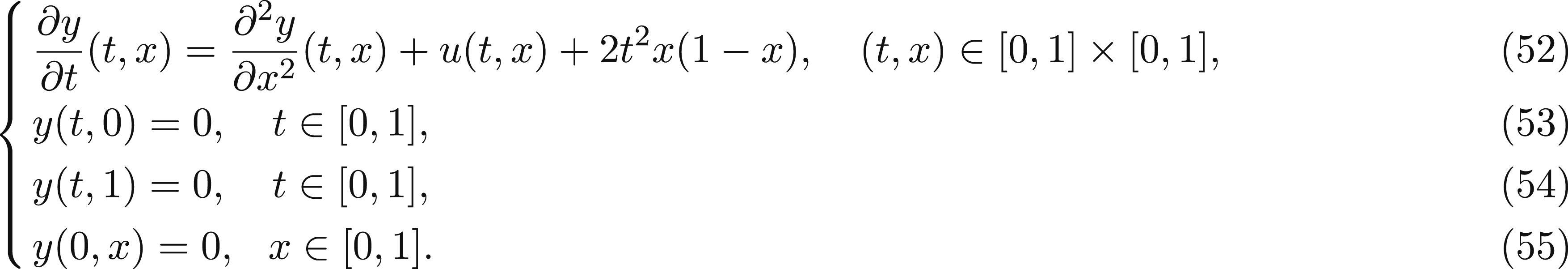
Consider the following OCP under PDEs
The exact optimal solutions of this problem are 

The analytical solution applies to the problem, enabling us to measure and validate the effectiveness of the proposed method and assess its error. The graphs depicting the results obtained from this method are as follows. Figures 1 and 2 display the approximate solutions the absolute errors for The approximate solution and the logarithm of absolute error between the approximate and exact state variables for The approximate solution and the logarithm of absolute error between the approximate and exact control variables for The logarithm of difference between exact and approximate solutions, in Example 1. The logarithm of The approximate value of 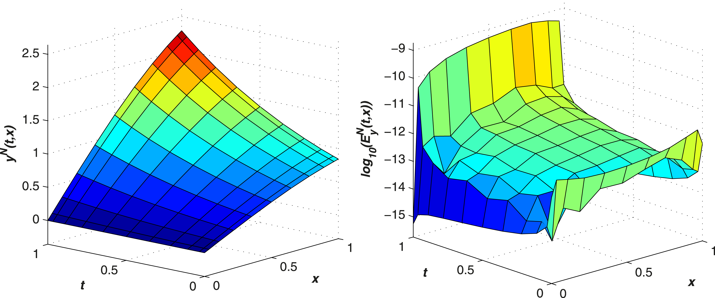
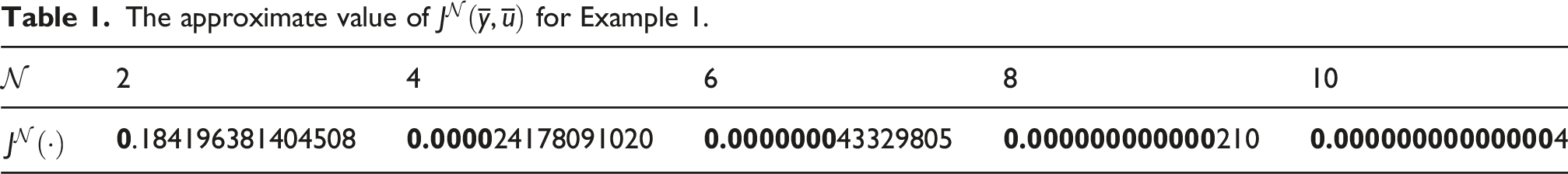
We note that
We consider the following OCP
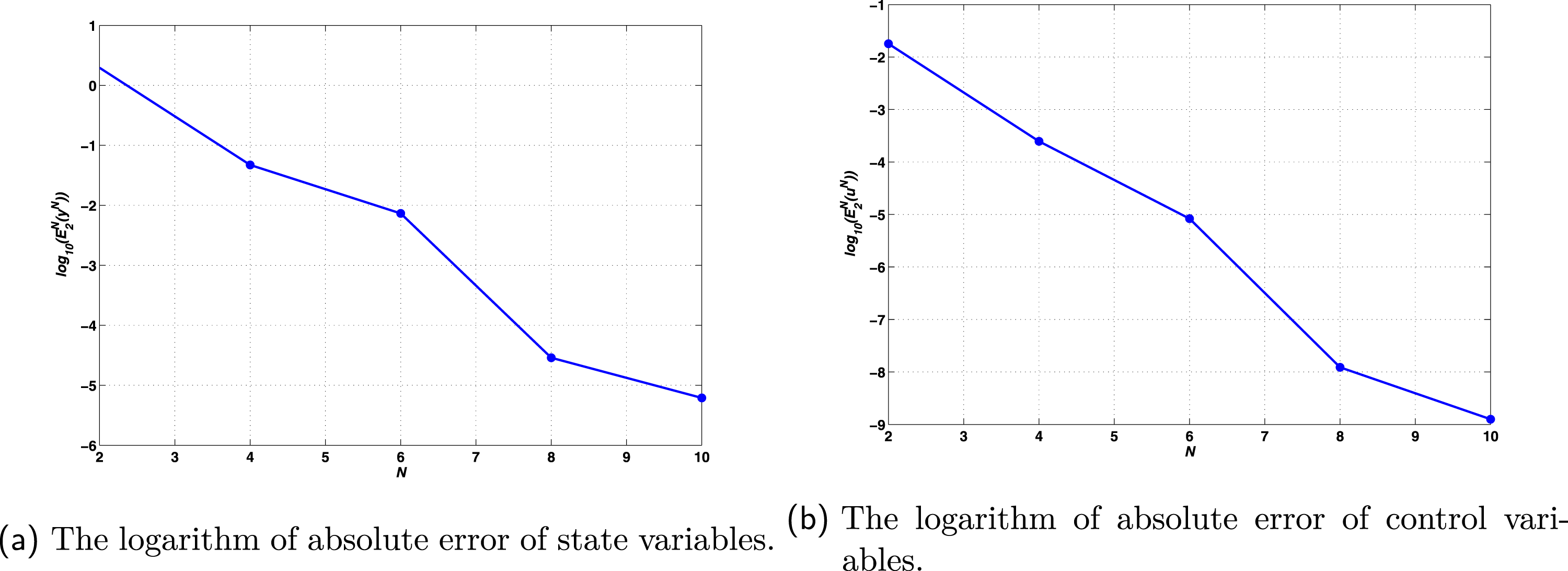
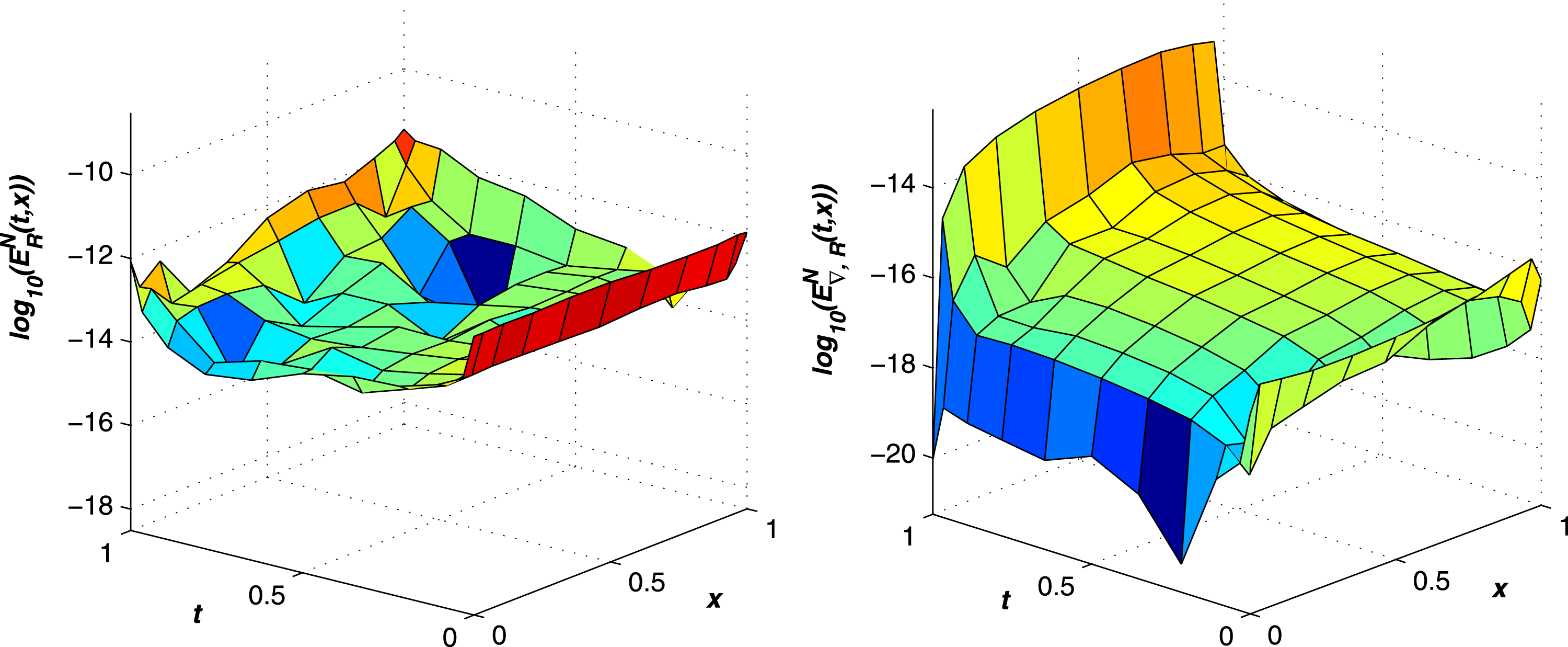
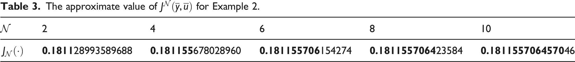
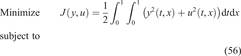
This problem has an optimal solution, but an analytical and precise relationship for it is not available. We solve this problem by presented approach. The approximate solutions for N = 20 are depicted in Figure 5. Moreover, Figure 6 illustrates the logarithm of the PDE residual error and the residual error of gradient equations. Upon examining the results presented in Tables 2 and 3, it becomes apparent that by increasing N, the absolute error reduces. The results obtained indicate the superiority and efficiency of LGL-PS method over VI method (Akkouche et al., 2014). The approximate solutions The logarithm of the The values of The approximate value of 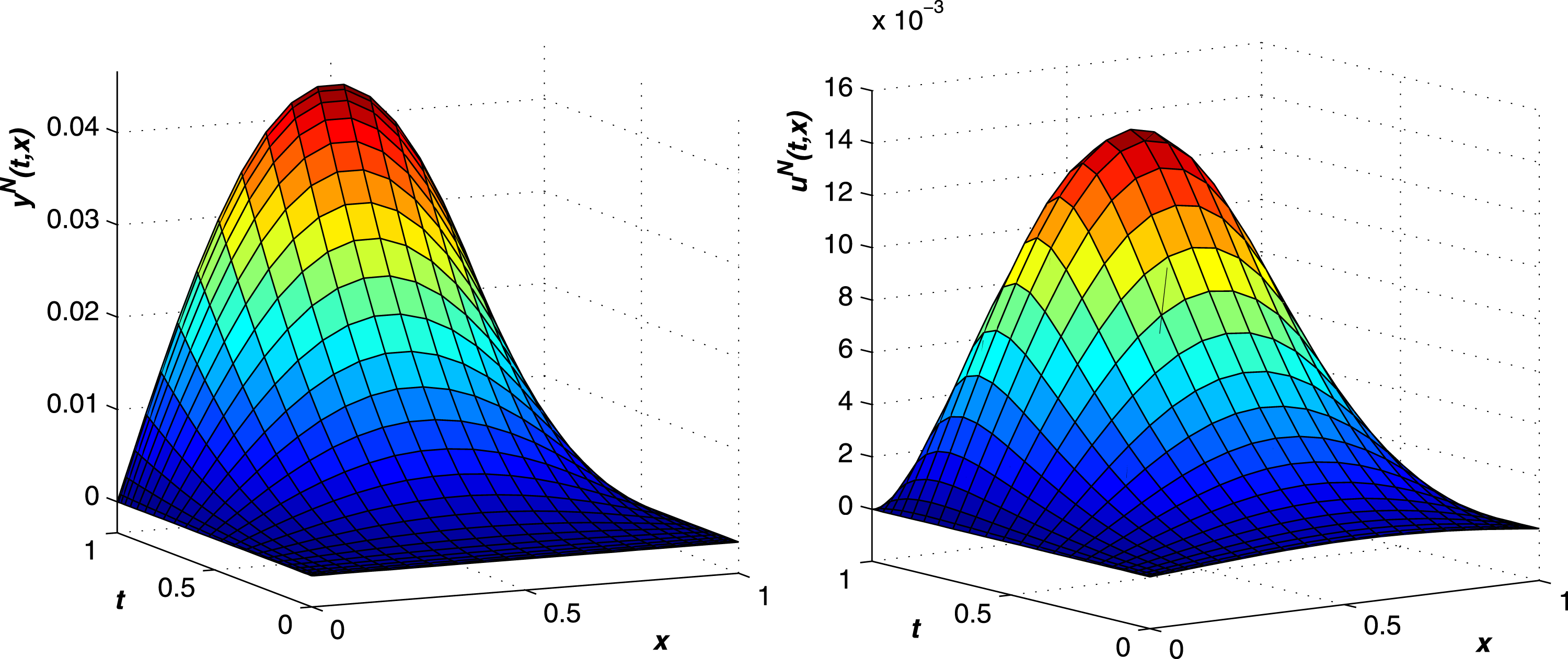
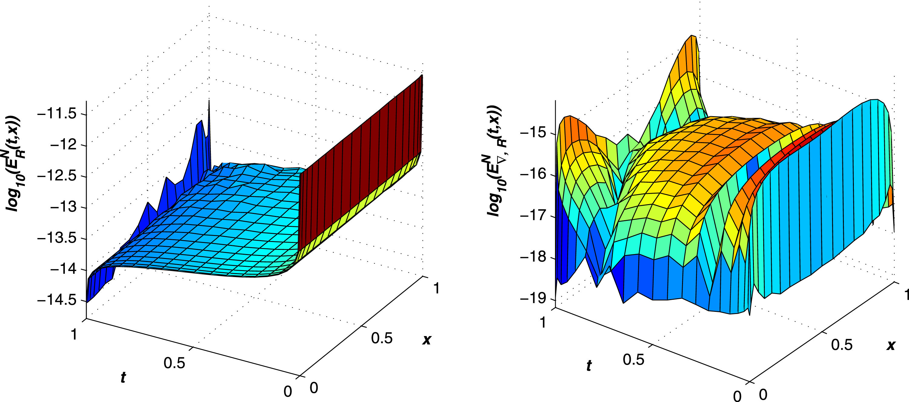
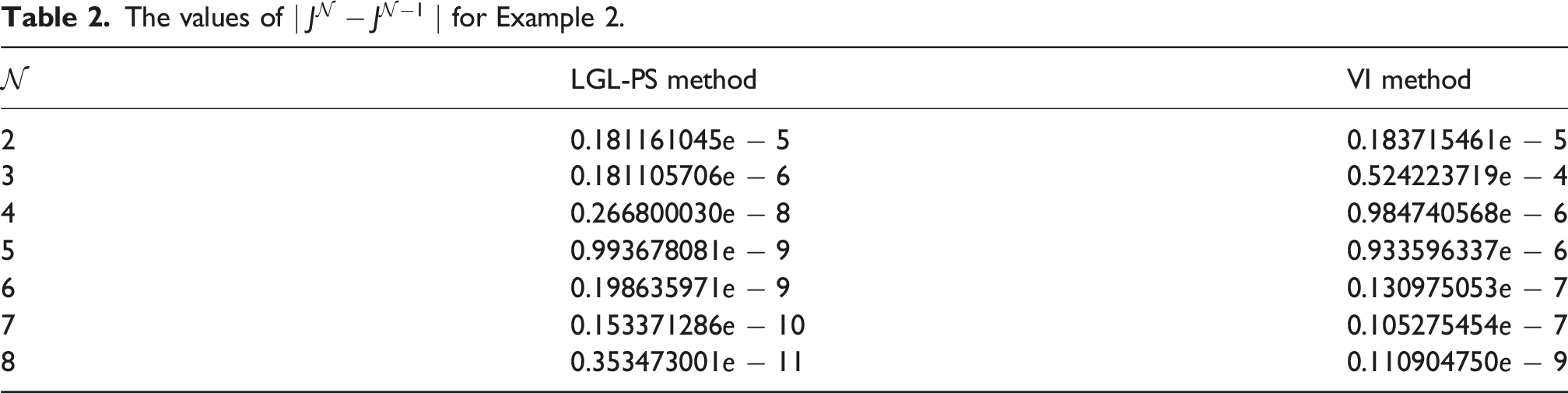
We note that Table 2, shows the residual values of the obtained numerical sequence. Given that the residual tends towards zero with increasing
Note that Table 3, represents a fixed number, and with each iteration, more digits of that number become constant with an increase of
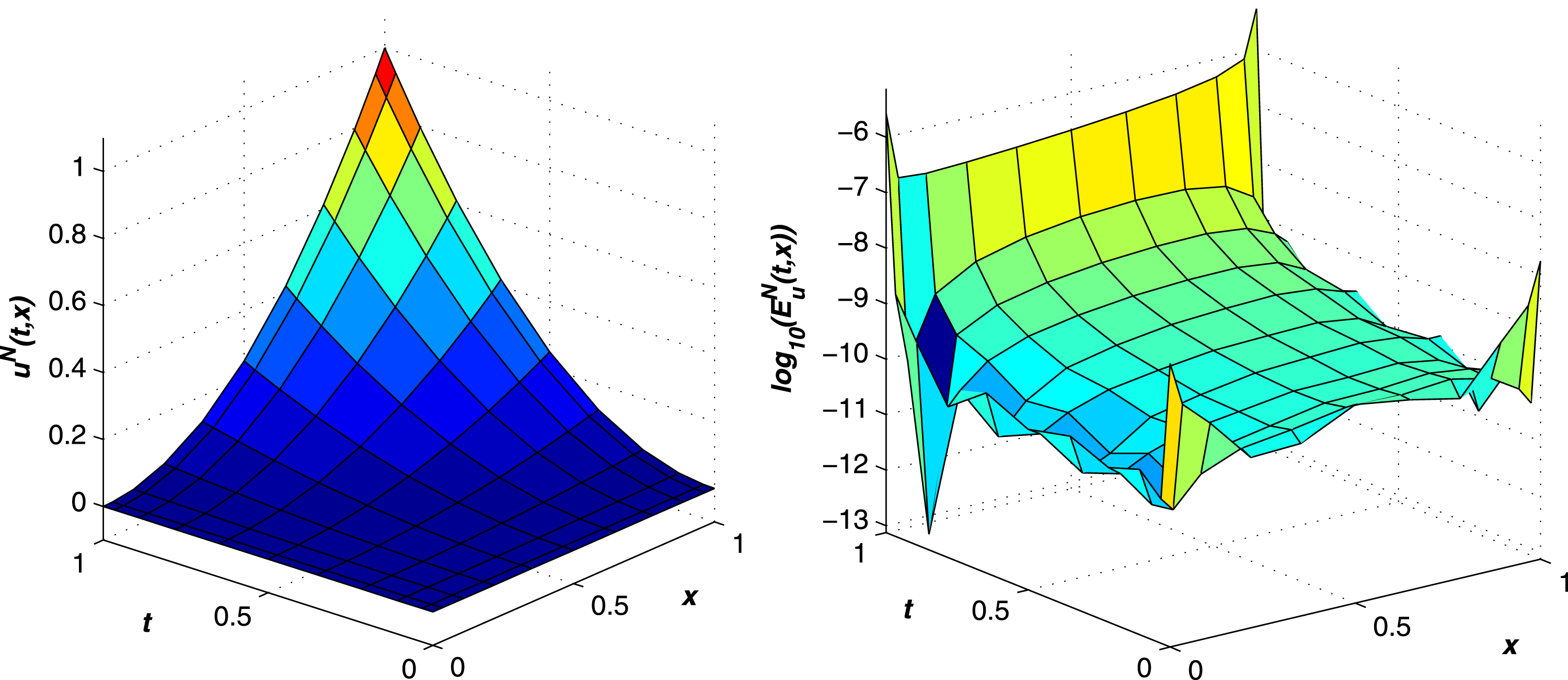
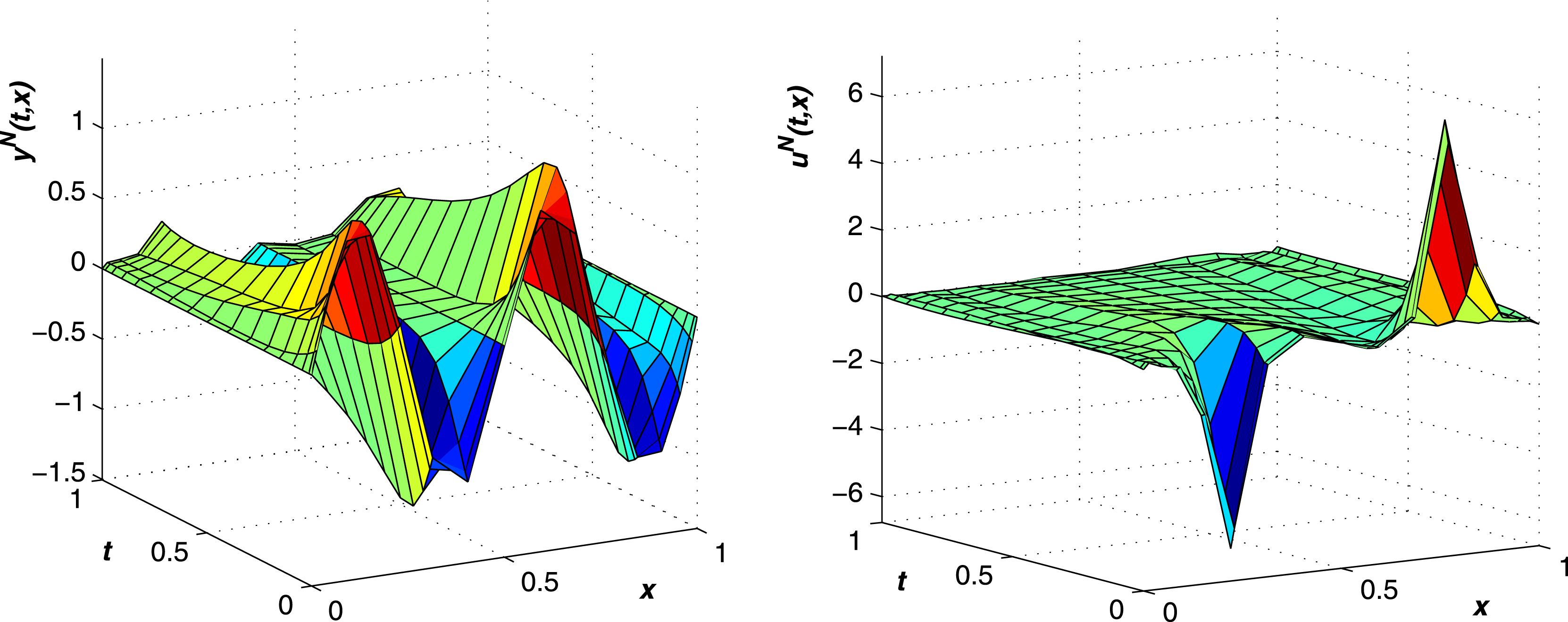
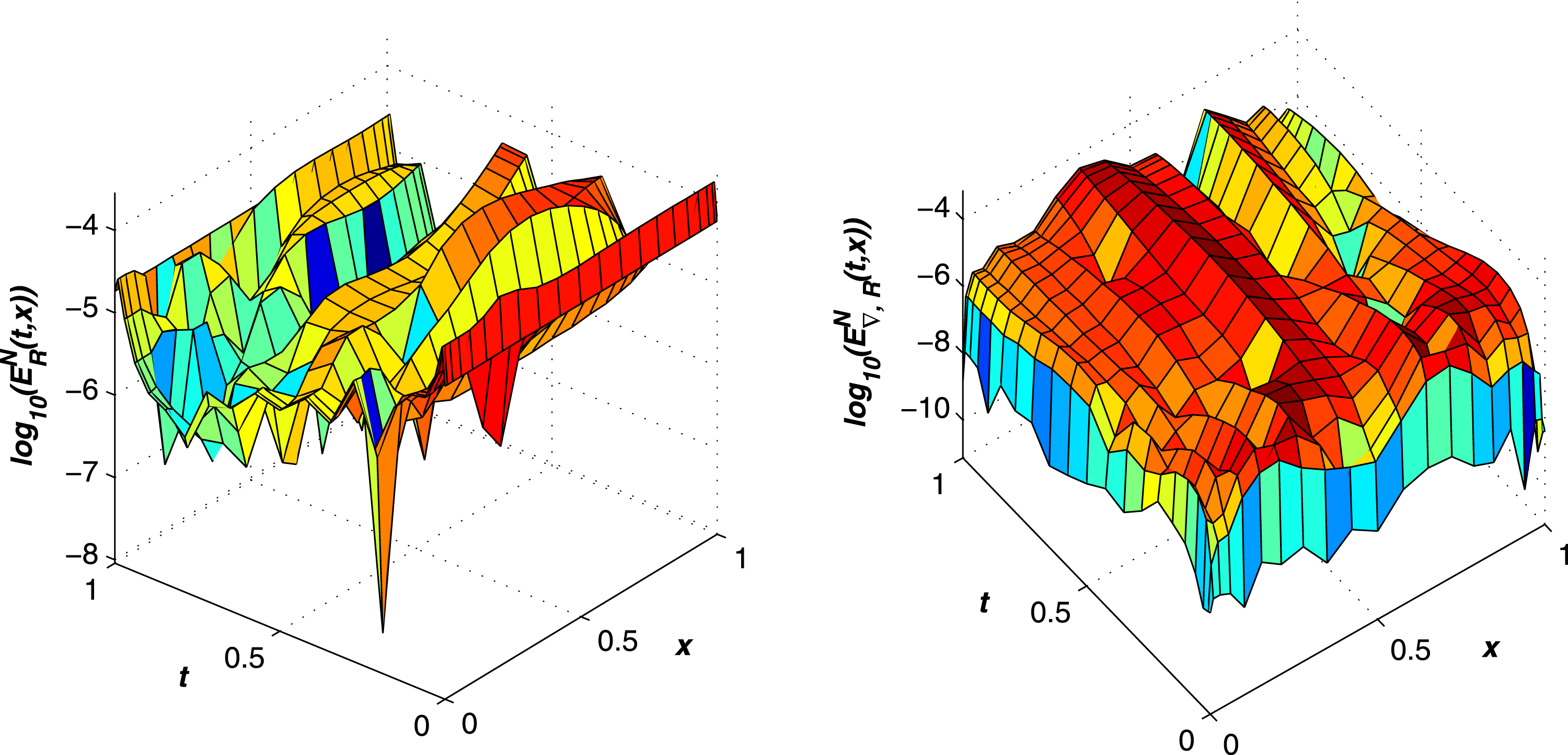
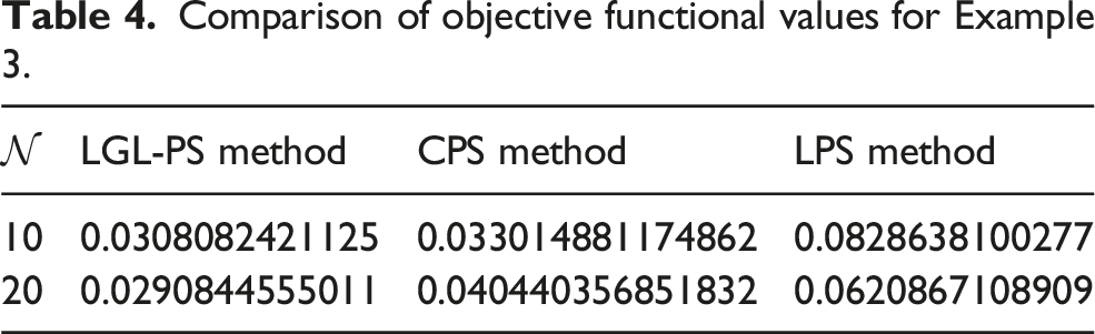
We consider the following OCP

This problem has an optimal solution, but an analytical form for it is not available. Hence, we solve this problem by our approach, numerically. For The approximate solutions The approximate solutions y
N
(t, x) and u
N
(t, x) with The logarithm of the The logarithm of the Comparison of objective functional values for Example 3.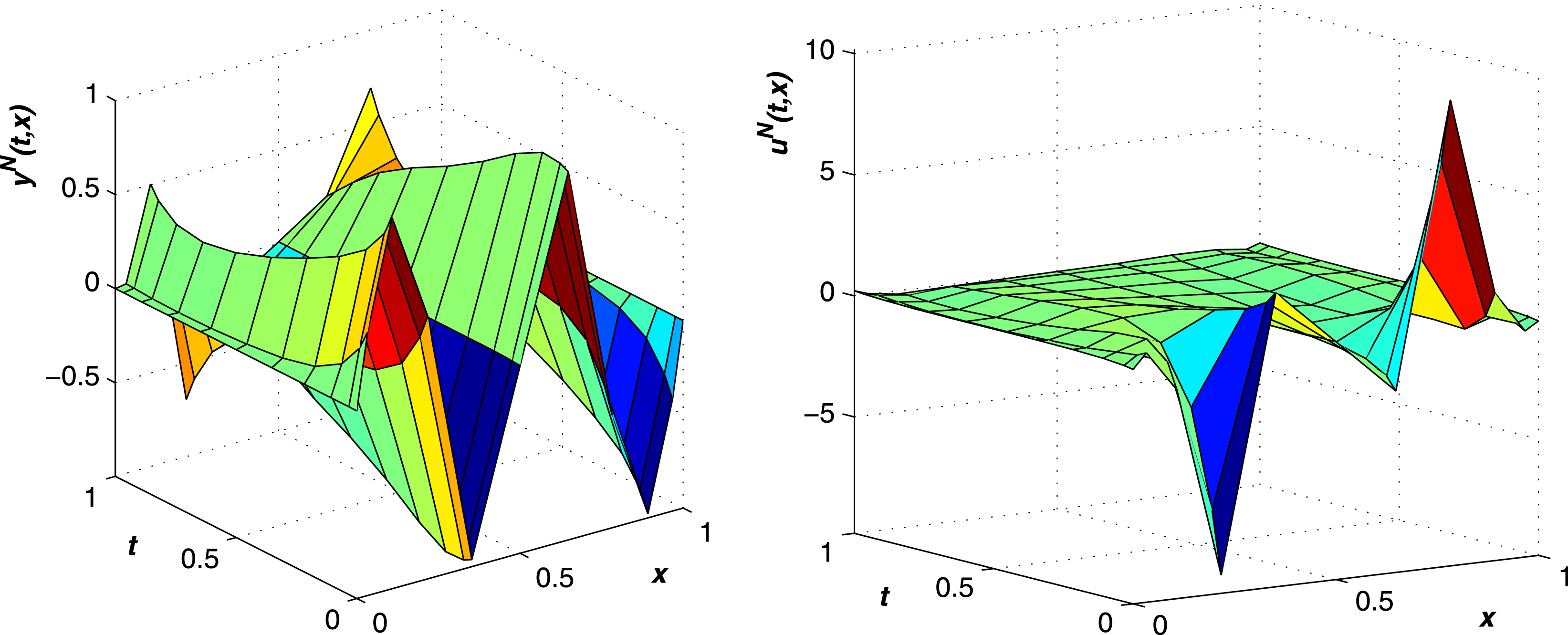
Conclusions and suggestions
In this paper, a novel and practical scheme was proposed for solving optimal control problems (OCPs) governed by partial differential equations (PDEs) using the Legendre–Gauss–Lobatto (LGL) pseudo-spectral (PS) method. The LGL-PS method has demonstrated significant advancements in the numerical solution of PDE-constrained OCPs, offering a robust combination of theoretical soundness, high-order accuracy, and computational efficiency. These features make it a valuable and versatile tool for addressing complex control problems in various scientific and engineering domains. Compared to existing numerical approaches, such as Legendre PS (LPS), Chebyshev PS (CPS), and variational iteration (VI) methods, the LGL-PS method yielded superior performance in terms of solution accuracy and error minimization, particularly for benchmark problems like the Burgers’ equation and the diffusion equation. The method’s ability to produce globally smooth and continuously differentiable approximations is crucial for ensuring reliable control strategies in dynamic systems. Furthermore, the proposed framework incorporates the Karush–Kuhn–Tucker (KKT) optimality conditions and employs efficient solvers such as the Levenberg–Marquardt algorithm, enabling the accurate resolution of the resulting nonlinear programming (NLP) problems. This integration enhances both the stability and convergence of the numerical scheme. The flexibility of the LGL-PS method suggests promising avenues for future research. In particular, extending this approach to OCPs governed by fractional-order PDEs, time-delay systems, and multi-dimensional nonlinear PDEs could significantly broaden its applicability. These problem classes are increasingly relevant in modeling complex phenomena such as anomalous diffusion, memory-dependent processes, and spatiotemporal dynamics in biological and physical systems. In summary, the LGL-PS method not only provides a powerful tool for solving classical PDE-constrained OCPs but also lays the groundwork for tackling emerging challenges in optimal control theory. Its continued development and adaptation to more generalized systems will be instrumental in advancing both theoretical insights and practical solutions in the field.
Footnotes
Funding
The author(s) received no financial support for the research, authorship, and/or publication of this article.
Declaration of conflicting interests
The author(s) declared no potential conflicts of interest with respect to the research, authorship, and/or publication of this article.
Data Availability Statement
There is no data out of the article to present.