
Abstract
This study presents an efficient computational fluid dynamics (CFD)-Beam theory time-frequency-domain hybrid method (TFDHM) to predict pipeline flow-induced vibrations (FIV). CFD is used to simulate the time-domain fluctuating pressure of the pipeline fluid, and the finite element method (FEM) based on Euler–Bernoulli beam theory is used to rapidly predict the frequency-domain vibration of the pipeline structure. A fluid load mapping method (FLMM) is introduced to convert the time-domain pressure into frequency-domain excitation load for application to a beam model. A curved pipeline FIV is simulated by the TFDHM. The results are compared with those calculated by the full-time-domain three-dimensional fluid-structure interaction method. It is found that the TFDHM is significantly more efficient than the FTDM, with a computation time of only 45 s versus 23 h 47 min for the FTDM. Furthermore, the influence of key factors on the TFDHM results is analyzed to optimize the FLMM. The accuracy of the numerical results is verified using the experimental results of the curved pipeline. In contrast, the TFDHM results have higher predictive reliability than those of FTDM under actual boundary constraints, which is because the former can use the measured frequency-domain dynamic stiffness of the pipeline support. Therefore, the TFDHM achieves computational accuracy equivalent to that of conventional methods while providing markedly improved computational efficiency and engineering applicability.
Keywords
Introduction
Fluid fluctuating pressure will cause vibrations in the pipeline structure. There vibrations may not only loosen connectors and damage precision instrument components but also contribute to noise pollution (Gao et al., 2016). Therefore, accurate and efficient prediction and analysis of flow-induced vibration (FIV) characteristics is essential in the design, optimization, and fault diagnosis of pipeline system to achieve low-vibration designs (Yu et al., 2022).
Primary computational methods for analyzing FIV in pipeline systems include the finite element method (FEM), the finite volume method (FVM), the transfer matrix method (TMM), the method of characteristics (MOC), MOC-FEM, and FVM-FEM (Li et al., 2014; EI et al., 2011; Veerapandi et al., 2014). Among these, FEM, FVM, MOC, MOC-FEM, and FVM-FEM usually solve the FIV responses in the time-domain (Adamkowski et al., 2010; Keramat et al., 2013). However, when introducing the mechanical impedance of elastic components as boundary conditions, these methods face challenges. This is because the mechanical impedance obtained from engineering experiments is typically represented in the frequency-domain. TMM can perform both time-domain and frequency-domain solution when studying the FIV characteristics (Gong et al., 2025). However, in the case of nonlinear flow, the calculation results of TMM often have large deviation. This is because TMM cannot accurately capture the characteristics of fluctuating pressure (Ferras and Didia, 2019). The full-time-domain three-dimensional fluid-structure interaction method (FTDM) based on FVM-FEM is now mainstream for computing FIV responses in pipelines (Liu et al., 2023; Zhang et al., 2025). This method employs CFD to calculate fluid flow within the pipeline and adopts FEM to solve structural vibrations in the time-domain. However, pipeline systems exhibit a chain-like configuration characterized by a large length-to-diameter ratio, diverse components, and complex spatial distributions. FTDM faces significant challenges in mesh and takes lengthy computation time for fluid load mapping. The time-frequency-domain hybrid method circumvents both obstacles by one-dimensional beam model and the fluid load mapping method. Overall, the primary computational methods are difficult to achieve a balance between computational efficiency and accuracy when solving pipeline FIV.
Fluid wall pressure serves as the excitation source of FIV in pipeline systems, its dynamic characteristics are crucial for accurately calculating these vibrations (Bachoo and Bridge, 2021). Computational fluid dynamic methods include direct numerical simulation (DNS), Reynolds-averaged Navier–Stokes (RANS), and large eddy simulation (LES) (Kumari et al., 2025). DNS directly solves the Navier–Stokes equations to capture fluid flow characteristics without the need for turbulence models. However, turbulence is an irregular, multi-scale, and nonlinear flow, high spatial and temporal resolutions are required to accurately capture its flow characteristics (Pianet et al., 2007). RANS simplifies the multi-scale characteristics of turbulent fluctuations by employing time-averaging. This approach necessitates only the calculation of mean fluid flow information, significantly enhancing computational efficiency. However, RANS focuses solely on the mean fluid flow information. Its computational accuracy is limited in engineering practice (Lopez-Santana et al., 2022). LES is an intermediate approach between DNS and RANS regarding computational efficiency and accuracy. This method classifies turbulence into large-scale and small-scale eddies using the filtering function. The motion of large-scale eddies is directly captured through the Navier–Stokes equation. Based on the sub-grid scale model, the influence of small-scale eddies on the motion of large-scale eddies is considered. This influence is introduced into the equation of large-scale eddy motion in the form of an additional stress term. Thereby, the indirect simulation of the effect of small-scale eddies is achieved (Chandragope and Hasan, 2014). LES has been widely used to accurately capture the fluctuating pressure characteristics within pipelines (Pittard and Blotter, 2003).
The primary methods for calculating pipeline vibration responses include the Galerkin method (GM), the transfer matrix method (TMM), the finite element method (FEM) (Han and Chi, 2024; Li et al., 2014; Liu et al., 2024; Qin et al., 2024a) and Spectral Element Method (SEM) (Qin et al., 2024b; Tran et al., 2025; Zhou et al., 2024, 2025). GM is effective for analyzing the vibration characteristics of simple pipelines. However, this method faces challenges in modeling and analyzing complex pipeline systems (Wu et al., 2025). TMM is effective for calculating the frequency-domain vibration responses of complex pipelines. However, ensuring computational accuracy is challenging when analyzing slender pipelines and higher-order vibration frequency issues (Deng et al., 2024). The FEM based on beam theory offers significant advantages in pipeline vibration analysis. It simplifies geometry and reduces computational cost while maintaining accuracy (Xu and Yang, 2004). Beam theory primarily includes the Euler–Bernoulli and Timoshenko types. The Euler–Bernoulli beam theory assumes that the cross-section remains perpendicular to the centroidal axis before and after deformation and that no axial strain occurs. It is suitable for slender beams. The Timoshenko beam theory, which accounts for shear deformation and rotational inertia in addition to the assumptions of the Euler–Bernoulli beam theory, is suitable for short and thick beams (Li et al., 2011, 2015). Considering the large length-to-diameter ratio of the pipeline, the FEM based on Euler–Bernoulli theory is employed to the vibration responses of the pipeline.
This study uses a curved pipeline as an example. The LES turbulence model is employed for numerical simulations to obtain the wall fluctuating pressure. An effective fluid load mapping method is introduced to obtain the excitation source of FIV. Combined with the FEM based on Euler–Bernoulli beam theory, a time-frequency-domain hybrid method for rapidly predicting the FIV of the pipelines is established. The accuracy and efficiency of this method is evaluated by comparison with the FTDM. The Influence of key factors on calculation results of this method is analyzed to optimize the FLMM. By comparing the calculation results with experimental results, the accuracy of the calculation results is verified. The influence of using the frequency-domain data obtained from experiments as boundary conditions on the computational accuracy is analyzed.
Basic theory
Based on the LES turbulence model, the unsteady Navier–Stokes equations are solved to obtain time-domain fluctuating pressures. The vibration control equations derived from Euler theory are discretized by the FEM to establish a one-dimensional pipeline model. The time-domain fluctuating pressures are converted into frequency-domain concentrated loads through segmented integration and Fourier transform, enabling the prediction of FIV responses at key measurement points.
Governing equation and large eddy simulation (LES) for incompressible fluid flow
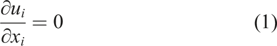
This study conducts an investigation into the FIV of liquid-filled pipelines. The governing equations of the flow field include the continuity equation and the momentum conservation equation. The fluid medium is water, where the density ρ
f
is a constant. The continuity equation is expressed as follows:
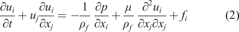
The momentum equation is
By spatial filtering to divide the turbulence into large-scale and small-scale eddies, the governing equations for large eddy simulation are derived as follows:
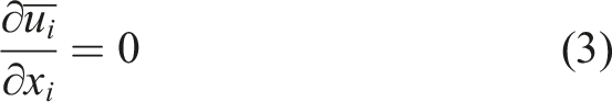
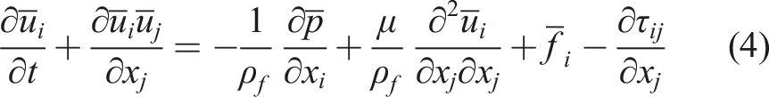
By solving the above governing equations, the velocity and pressure are obtained. Subsequently, the fluctuating pressure on the fluid wall are extracted and utilized as the excitation load for FIV.
Vibration governing equation based on Euler beam theory
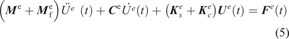
The FEM based on Euler–Bernoulli beam theory is employed to solve the vibration characteristics of liquid-filled pipeline with circular cross-section. The pipeline is discretized into n pipeline elements, as depicted in Figure 1. By applying Hamilton’s principle, the finite element equations for the liquid-filled pipeline elements in the state of motion can be derived: Beam models of the curved pipeline.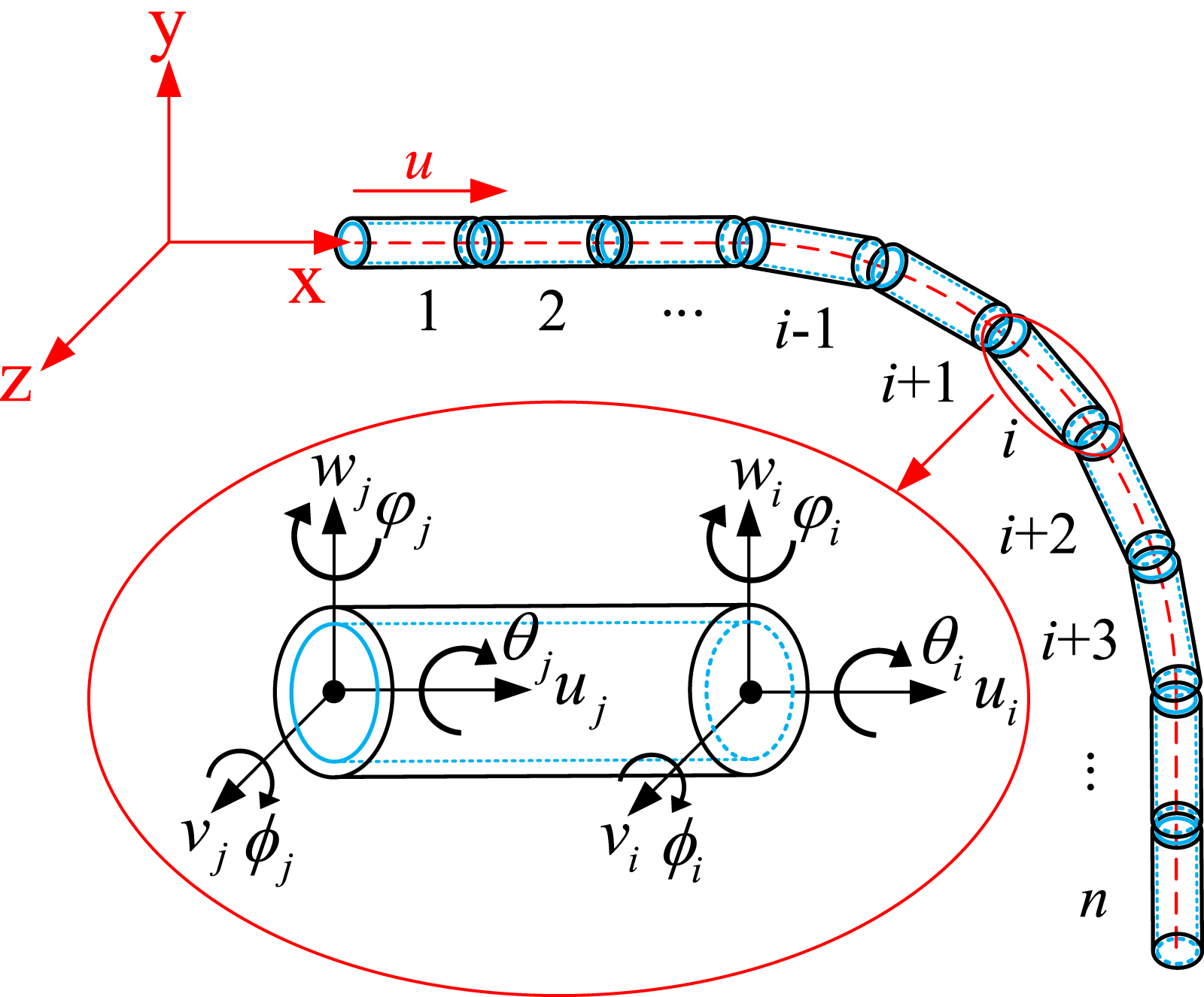

The Rayleigh damping matrix can be expressed as

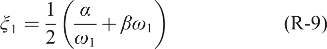
In general, the coefficients α and β are determined from the modal damping ratios. According to the orthogonality principle, the first-order modal damping ratio ξ
1
and the corresponding natural frequency ω
1
satisfy the following relation:
For the structure, the first- and second-order natural frequencies are ω
1
and ω
2
, with the corresponding modal damping ratios ξ
1
and ξ
2
, respectively. Then, the following relations hold:
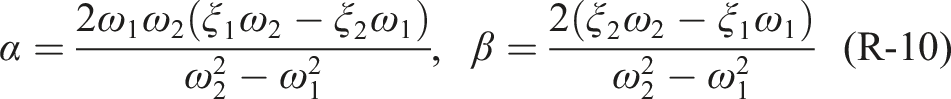
In this study, the pipeline material is structural steel, and the modal damping ratios are specified as ξ 1 = 2% and ξ 2 = 3%.
The finite element motion equation of the overall pipeline is obtained by integrating the element motion equations. By utilizing the Fourier transform, the dynamic equation of the pipeline structure in the frequency-domain can be derived:

This study establishes a FEM for pipeline dynamics based on the Euler–Bernoulli beam theory. To ensure model solvability and computational efficiency, several assumptions are inevitably introduced, which lead to the following limitations: (i) The pipeline is idealized as a circular tube with uniform cross-section, purely elastic, homogeneous, and isotropic, without considering the effects of material nonlinearity, cross-sectional variations, or welds on the dynamic behavior. (ii) Radial fluid motion and rotation around the pipe axis induced by transverse pipe deformation are neglected, and thus, the complex three-dimensional fluid-structure interaction effects are not fully captured. (iii) The frictional coupling between the pipe wall and the fluid is not considered, which may lead to underestimation of energy dissipation and damping characteristics. (iv) The internal fluid is assumed to be single-phase without cavitation, excluding more complex flow conditions such as multiphase flows or cavitating flows. (v) Pipe motion and deformation are limited to small displacements and small deformations, and large deformations or strongly nonlinear vibrations are not covered.
3D-1D time-frequency-domain hybrid method
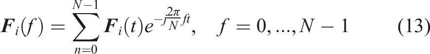
Establishing TFDHM requires addressing a key issue. This issue is how to convert the time-domain fluctuating pressure into the frequency-domain excitation load for FIV at the pipeline element level. This study uses the FLMM based on segmented integration and Fourier transform as the solution approach: (i) Considering the pipeline configuration and the intense spatio-temporal variations of the fluid wall fluctuating pressure, the pipeline is segmented along its axial direction. (ii) The time-domain fluctuating pressures of different pipeline segments are integrated along the wall surface. In accordance with the principle of force equivalence, it is ensured that the principal vector of the load obtained after integration is consistent with that of the original distributed load. (iii) Through Fourier transform, the time-domain fluid load is converted into frequency-domain fluid load. The complex form frequency-domain load is then utilized as the excitation for FIV, thereby taking into account the influence of phase differences among different excitation.
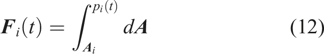
When applying the TFDHM for calculations, the following fundamental assumptions are introduced: (i) During the load mapping process, only the equivalent force assumption is employed, while the effect of moments is neglected. It is assumed that, when the pipeline is sufficiently finely discretized, the influence of moments on the calculation results can be ignored. (ii) Based on Saint-Venant’s principle, the load application location should be as far as possible from the measurement points to minimize the influence of the concentrated load application on the calculation results.
Comparison of the TFDHM and the FTDM
A computational model for the curved pipeline is established. The numerical boundary conditions are defined. The insensitivity to computational conditions is examined. The TFDHM and FTDM are used to solve the FIV responses, followed by a comparison and analysis. Subsequently, the influence of key FLMM factors on the TFDHM calculation results is analyzed.
Calculation model and numerical conditions
Model description
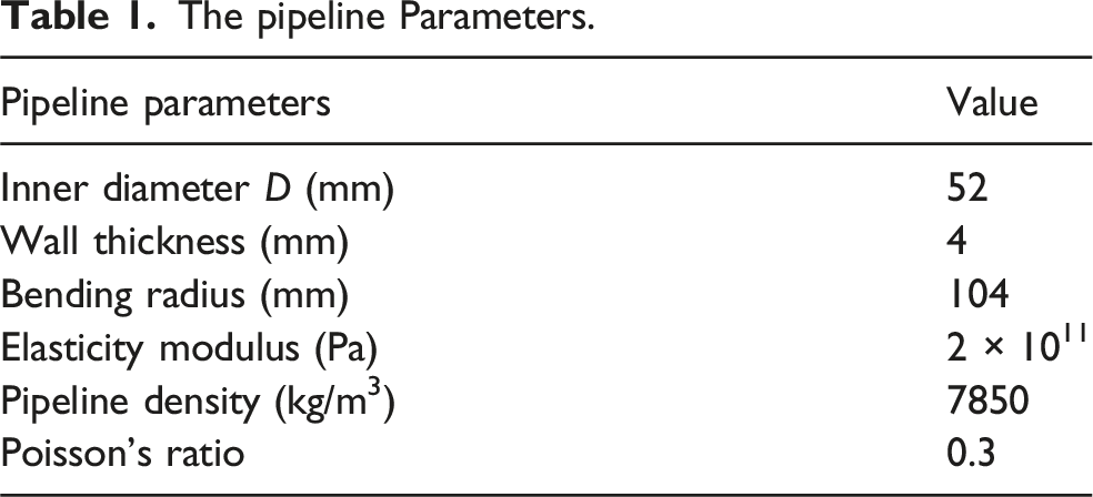
As depicted in Figure 2, this study focuses on a curved pipeline featuring a 90° elbow with straight pipes at both ends. This pipeline has an outer diameter of 60 mm, an inner diameter of 52 mm, and the bending radius of the elbow is 104 mm. To ensure a fully developed flow within the pipeline, both straight pipes are designed with a length of 1520 mm. Details of the curved pipeline.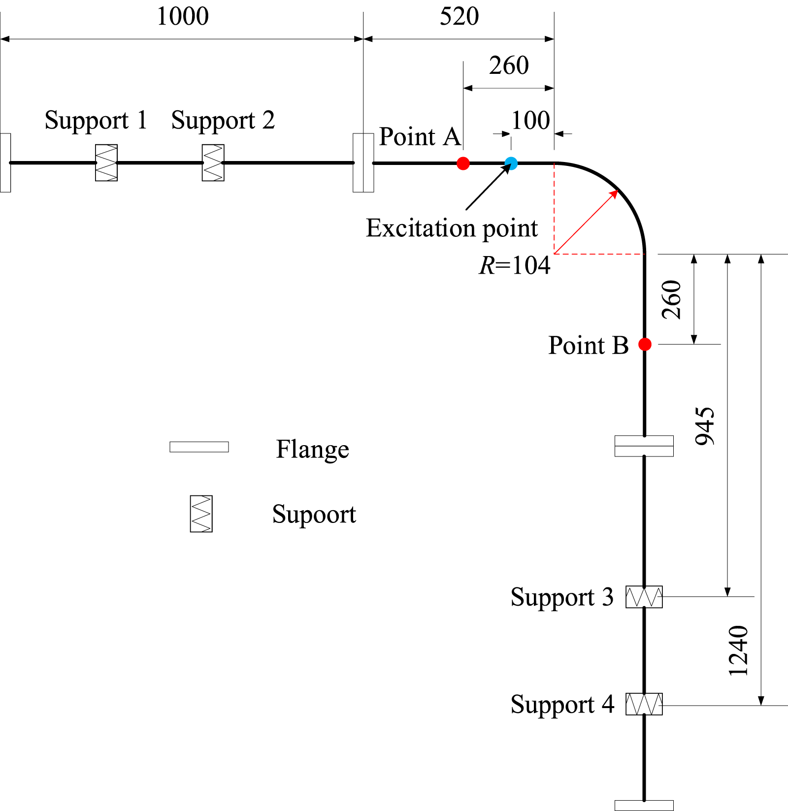
Mesh and boundary conditions
Fluid domain Mesh and boundary conditions
The fluid domain is discretized using hexahedral mesh with an O-type topology (illustrated in Figure 3). The mesh is refined near the wall, with the height of the first layer set at 0.003 mm and a growth rate of 1.2. The total mesh consists of 2,334,366 elements, all with a quality above 0.45. Considering the subsequent transient calculations using the LES turbulence model, the wall Y+ value is maintained below 1. Fluid domain mesh model.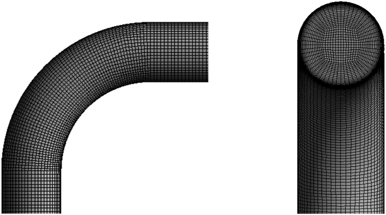
Water is used as the fluid medium (density: 998.2 kg/m3; viscosity: 0.001 kg/(m·s)). With the inlet velocity and outlet pressure specified as boundary conditions, the inlet velocity is set to 4.9 m/s and the outlet pressure to 0 Pa. A no-slip condition is applied to all wall surfaces.
Firstly, a steady flow field computation is conducted using the Standard k-ε turbulence model. Subsequently, a transient flow field computation is conducted based on the LES turbulence model to obtain the wall fluctuating pressure.
Structural domain Mesh and boundary conditions
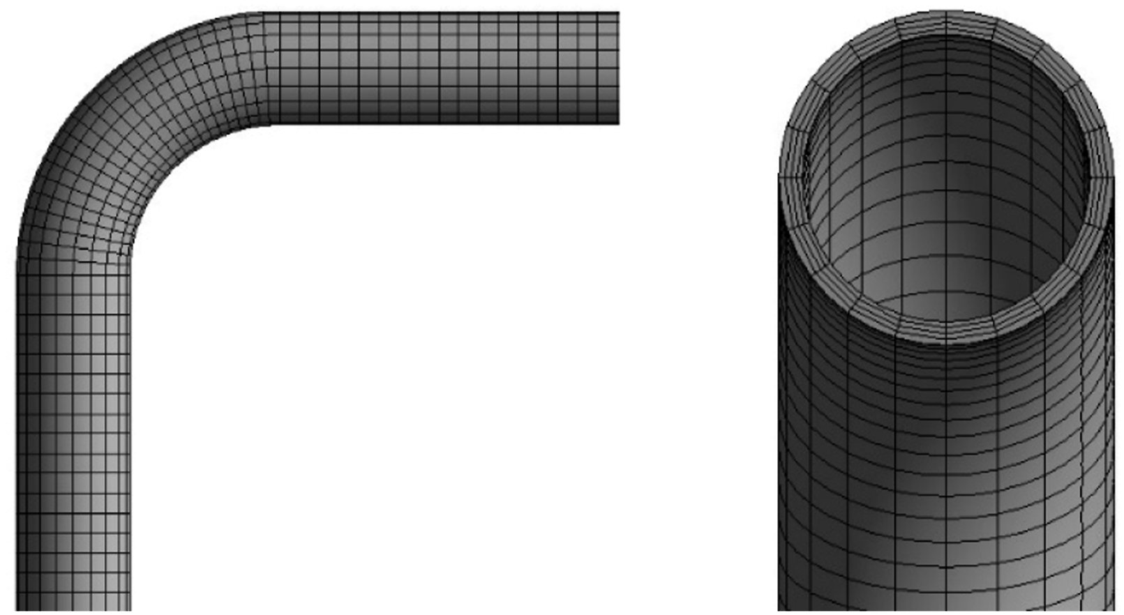
Figure 4 presents the 3D model of the structure and its simplified 1D beam element model. The 3D model is meshed with hexahedral solid elements, with the pipeline wall thickness is divided into 4 layers to enhance mesh resolution, resulting in a total of 96,616 elements (Figure 5). Geometric simplification and Segmentation. Structural domain mesh model.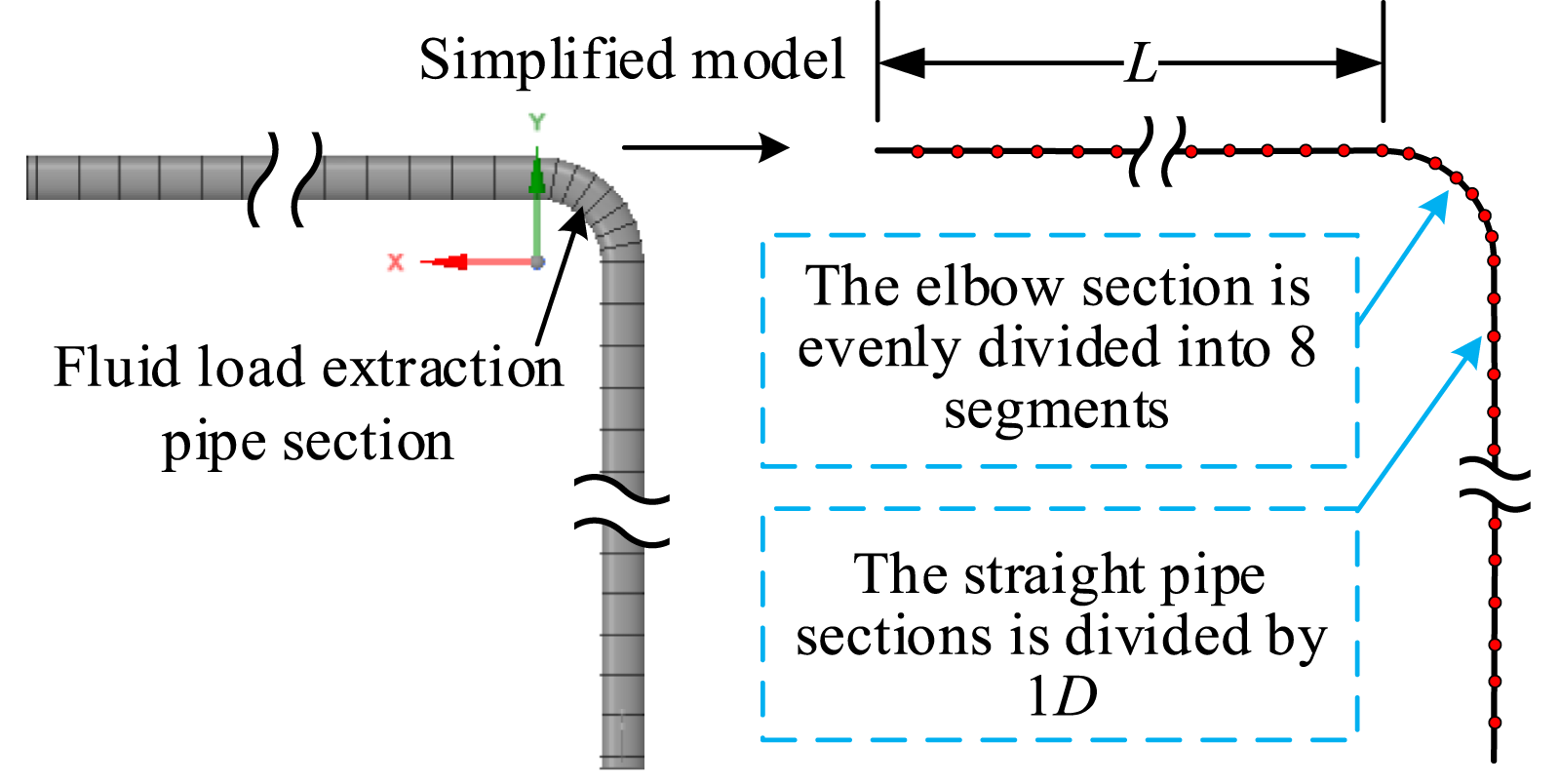
The pipeline Parameters.
Results and analysis
Analysis of insensitivity to computational conditions
Mesh independence analysis
A comparison of fluid load (the fluid load is the concentrated force at the third section of the inlet of the elbow shown as Figure 4) results under different mesh densities (approximately 1 million, 2.3 million, and 4 million cells) is provided (Figure 6), demonstrating that the selected mesh achieves convergence. The comparison of frequency-domain load spectra indicates that when the mesh contains approximately 2.3 million elements, the results are essentially consistent with those obtained using a finer mesh (approximately 4 million elements), with good convergence in both spectral amplitude and distribution characteristics. Therefore, a mesh of approximately 2.3 million elements is selected in this study, which ensures computational accuracy while significantly reducing computational cost.
Time-step sensitivity analysis
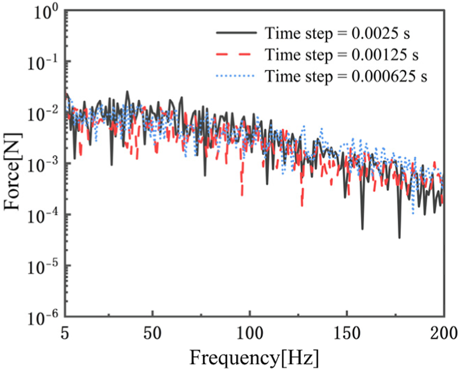
A comparison of fluid load results under different time steps (0.0025 s, 0.00125 s, and 0.000625 s) are provided, demonstrating that the time-domain resolution and frequency-domain stability of the fluctuating load data. The comparison of frequency-domain load spectra indicates that the calculation results are essentially consistent across different time steps, indicating that the selected time step (0.00125 s) ensures both sufficient time-domain resolution and frequency-domain stability of the fluid load data (Figure 7). Comparison of different mesh densities. Comparison of different time steps.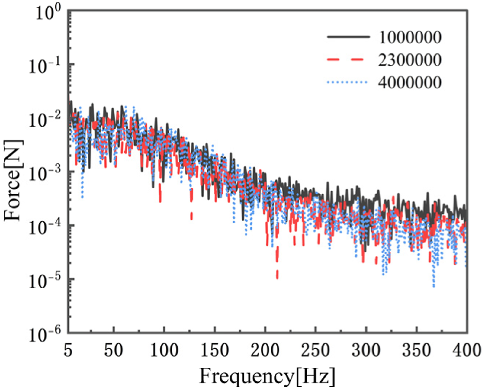
Comparison of the results by different methods
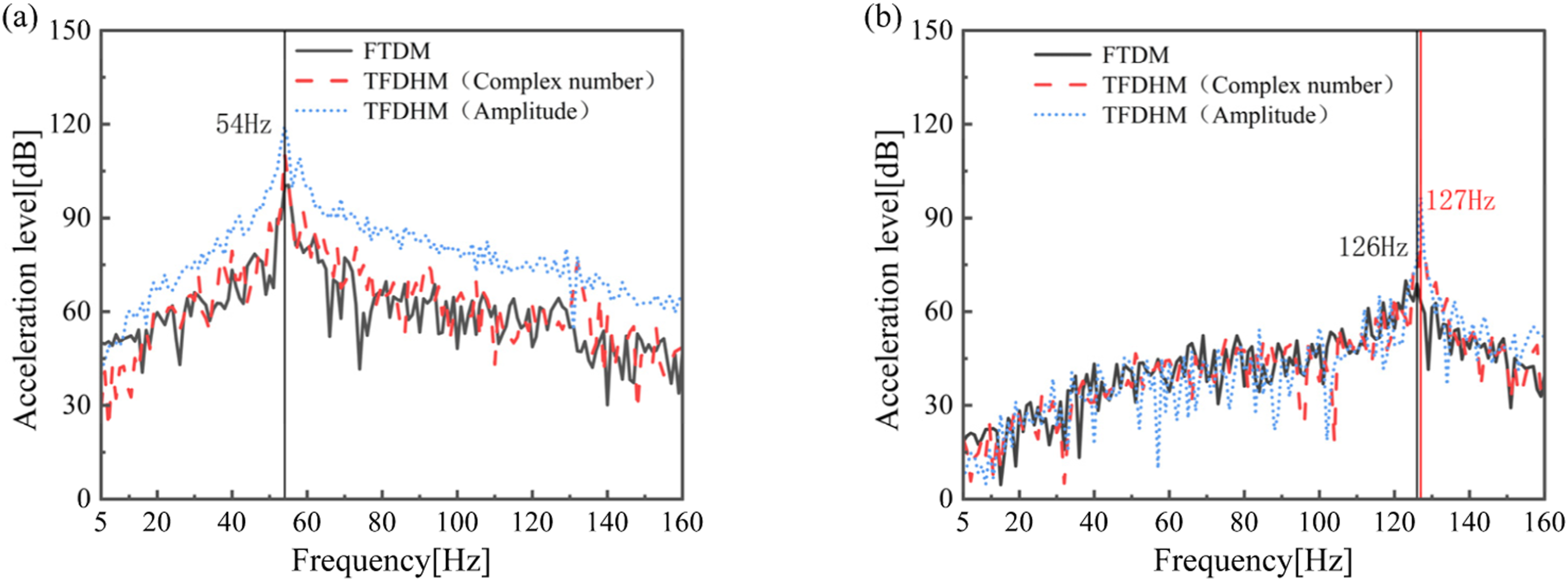
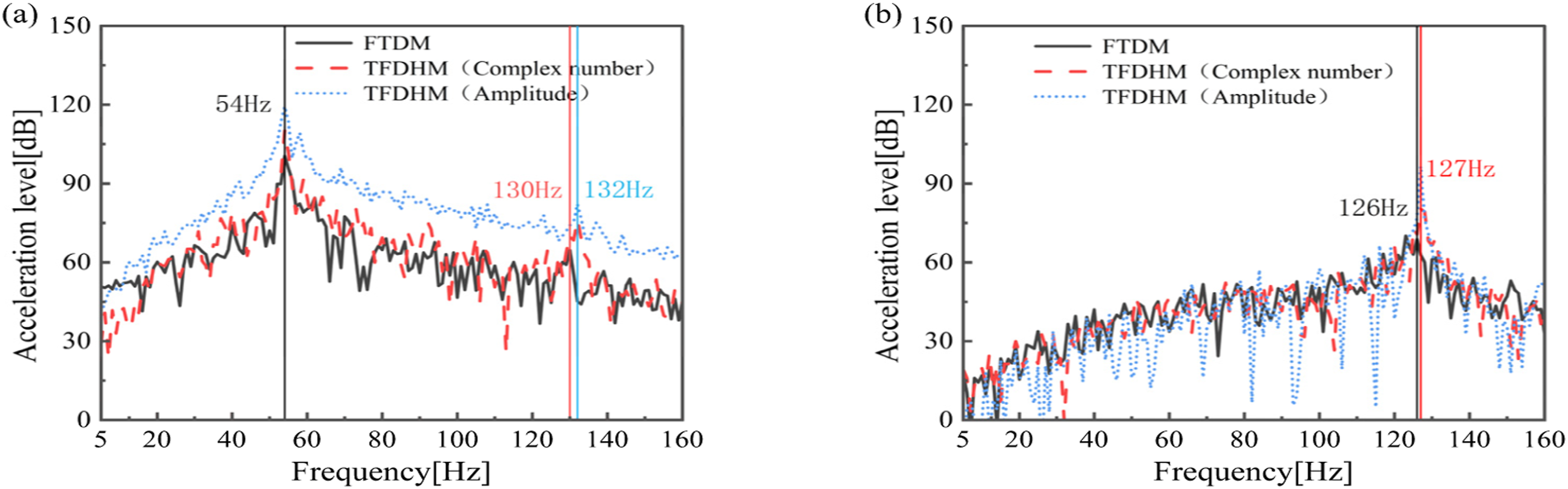
The CFD calculations show that the strong vortex area exhibits pronounced local concentration, thereby inducing strong fluctuating pressure within this area. Its main distributed location is at the elbow section, as shown in Figure 8. The amplitude of the fluctuating pressure predominantly falls within the frequency range of 5 ∼ 160 Hz. In this study, this frequency range is considered as the effective frequency band. The fluid load originating from the elbow section is used as the excitation, and the elbow section is discretized into eight segments. The FIV responses calculated by the TFDHM and the FTDM at various measurement points (illustrated in Figure 2) are presented in Figures 9 and 10. In this analysis, when the phase is considered, the excitation is calculated using the complex load as given in equation (9); when the phase is not considered, the excitation is calculated using the load amplitude as given in equation (9). Vorticity magnitude distribution. Comparison of acceleration level by the TFDHM and the FTDM at point A: (a) vertical direction and (b) transverse direction. Comparison of acceleration level by the TFDHM and the FTDM at point B: (a) vertical direction and (b) transverse direction.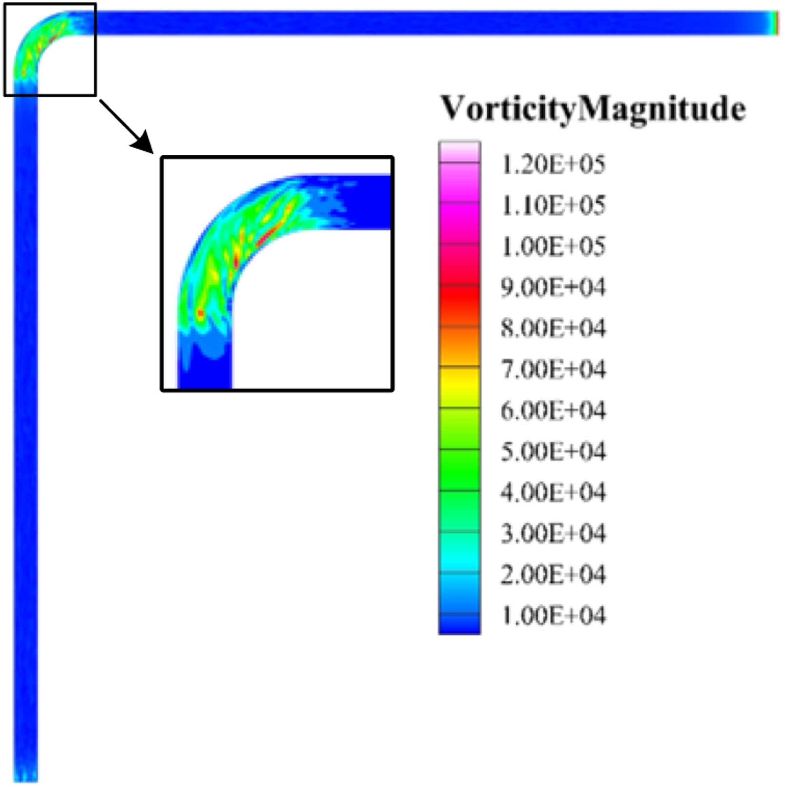
Comparison of overall acceleration level by the TFDHM and the FTDM.
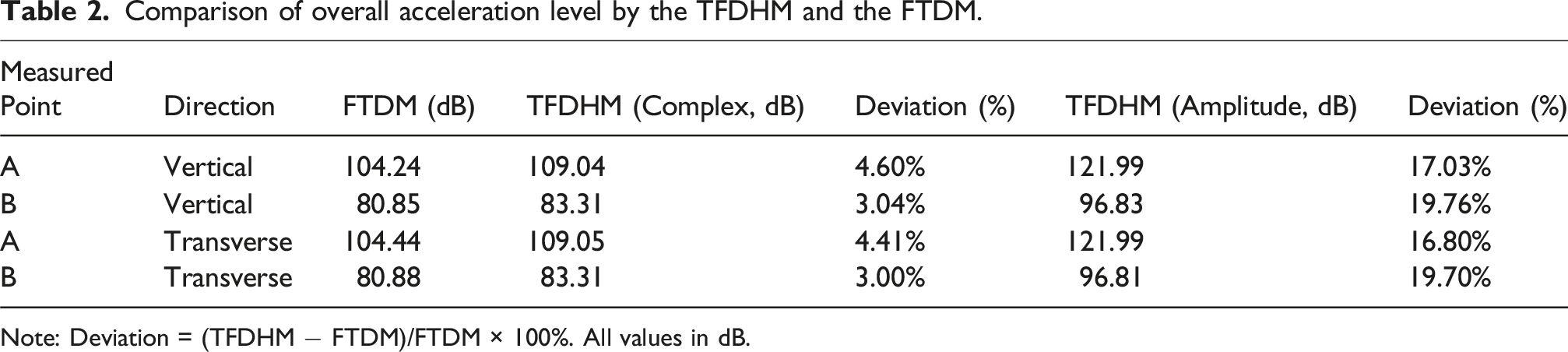
Note: Deviation = (TFDHM − FTDM)/FTDM × 100%. All values in dB.
The flow field computational time is identical for both methods. The solution of the structural response using the TFDHM costs 45 seconds, while it takes 23 hours and 47 minutes using the FTDM. It is found that TFDHM has a much shorter structural response computational time than FTDM. Therefore, the proposed TFDHM markedly enhances the computational efficiency of pipeline FIV while maintaining same accuracy as FTDM. Furthermore, the FIV response trends at point A and point B are highly similar. In Section 3.2.2, only point A is selected as the representative indicator for analysis.
Influence of FLMM key factors on calculation results of the TFDHM
Influence of pipeline segmented scales
To investigate the influence of various segmented scales on the calculational accuracy, multiple pipeline segmented scales are implemented. The elbow section is discretized into two, three, four, eight, and 16 segments (N = 2, 4, 8, 16). The excitation load within the elbow section is extracted. Figure 11 presents a comparison of FIV responses at each measurement point calculated by the TFDHM. When the elbow section is discretized with N = 2 or N = 4, the transverse FIV response is consistent with the FTDM results, but the longitudinal FIV response is significantly lower in the frequency range of 20 ∼ 110 Hz. As the number of segments N increases, the TFDHM results show a trend toward convergence. This deviation may be attributed to the conversion of distributed loads into concentrated loads through integration. This method preserves the resultant force but introduces a moment discrepancy at the application point (this moment discrepancy not considered in this study). As the number of segments increases (N ≥ 8), the elbow segments shorten, the moment decreases, and the approximate calculation results of the FIV response converge. Comparison of acceleration level under various pipeline segmented scales: (a) at point A in vertical direction and (b) at point A in transverse direction.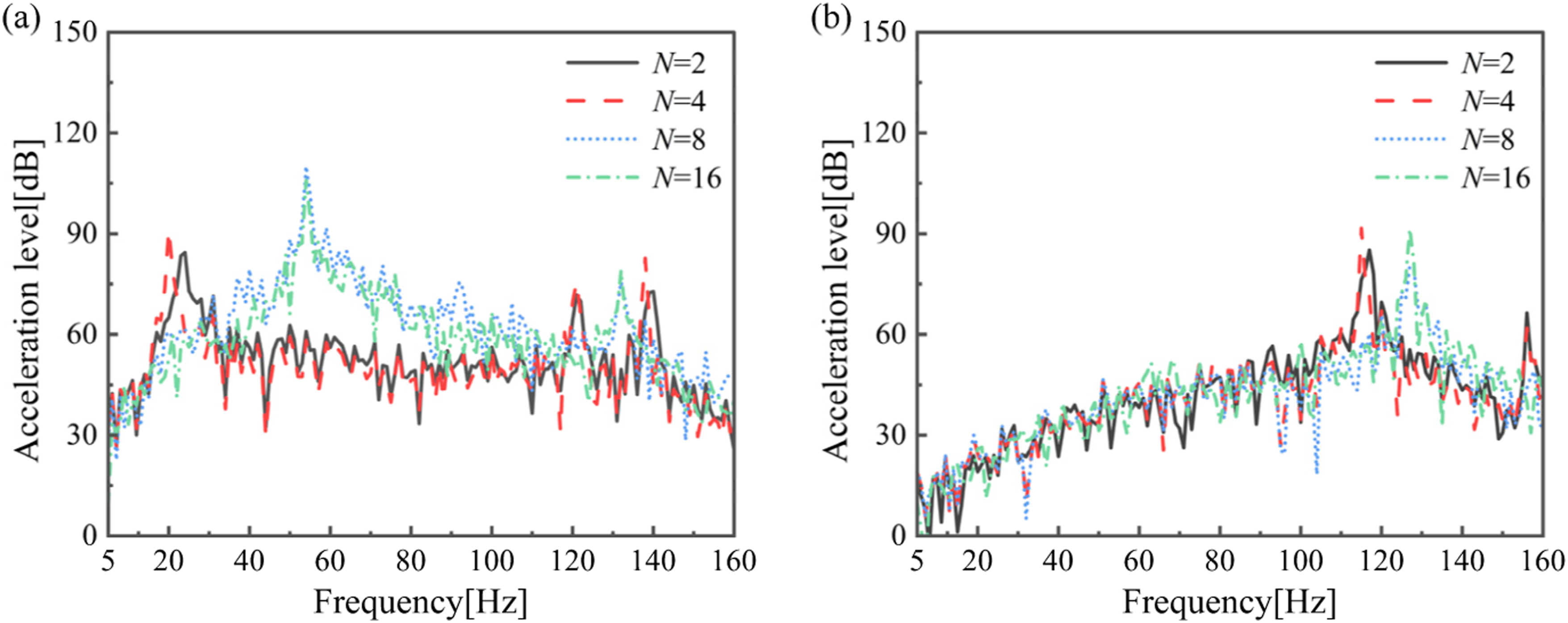
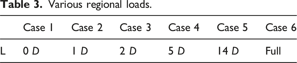
Influence of the fluid load
Various regional loads.
Comparison of acceleration level under various regional loads: (a) at point A in vertical direction and (b) at point A in transverse direction.
Experimental verification
An FIV experiment is conducted on a 90° elbow pipeline. The measured dynamic stiffness is taken as the boundary condition for the pipeline support. The accuracy and engineering practicality of TFDHM are verified.
Test rig of pipeline with a 90° elbow
To verify the computational accuracy of the TFDHM, the pipeline with a 90° elbow FIV experiment is conducted. The pipeline experimental system primarily consists of a gravity-fed water tank, ball valves, buffer tanks, a flowmeter, pressure gauges, exhaust valves, flexible tubes, pipeline supports, an experimental parameter measurement system, and other accessories, as shown in Figure 13. Experimental setup.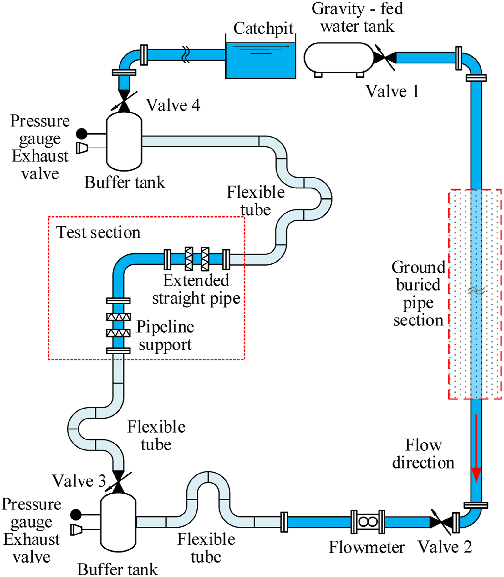
The gravity-fed water tank supplies water to the pipeline system, with Valve 2 adjusting the flow rate. To reduce incoming flow vibration and noise, 10-m flexible tubes are installed both after Valve 2 and before/after the test section, along with buffer tanks positioned upstream and downstream of the test section. As illustrated in Figure 2, accelerometers are mounted on the test section. The accelerometers are instrumented with BK A4534-B-001 models, which are connected to the computer by BK 3053-B-120 signal analyzer. The acceleration signals are obtained, converted, and stored by Labshop software, which are used to verify the computational methods.
The Photo of the test section is shown in Figure 14. The flow conditions and pipeline geometry are Consistent with the numerical conditions. In the experiment, the actual pipeline supports are used for fixation. The TFDHM takes the measured dynamic stiffness as the boundary constraints for the pipeline supports. Photo of the curved pipeline.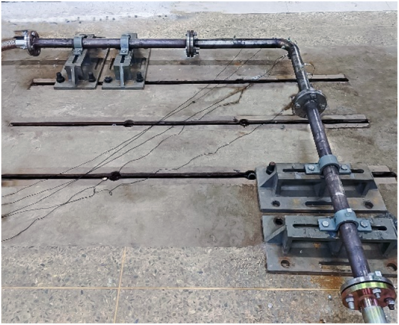
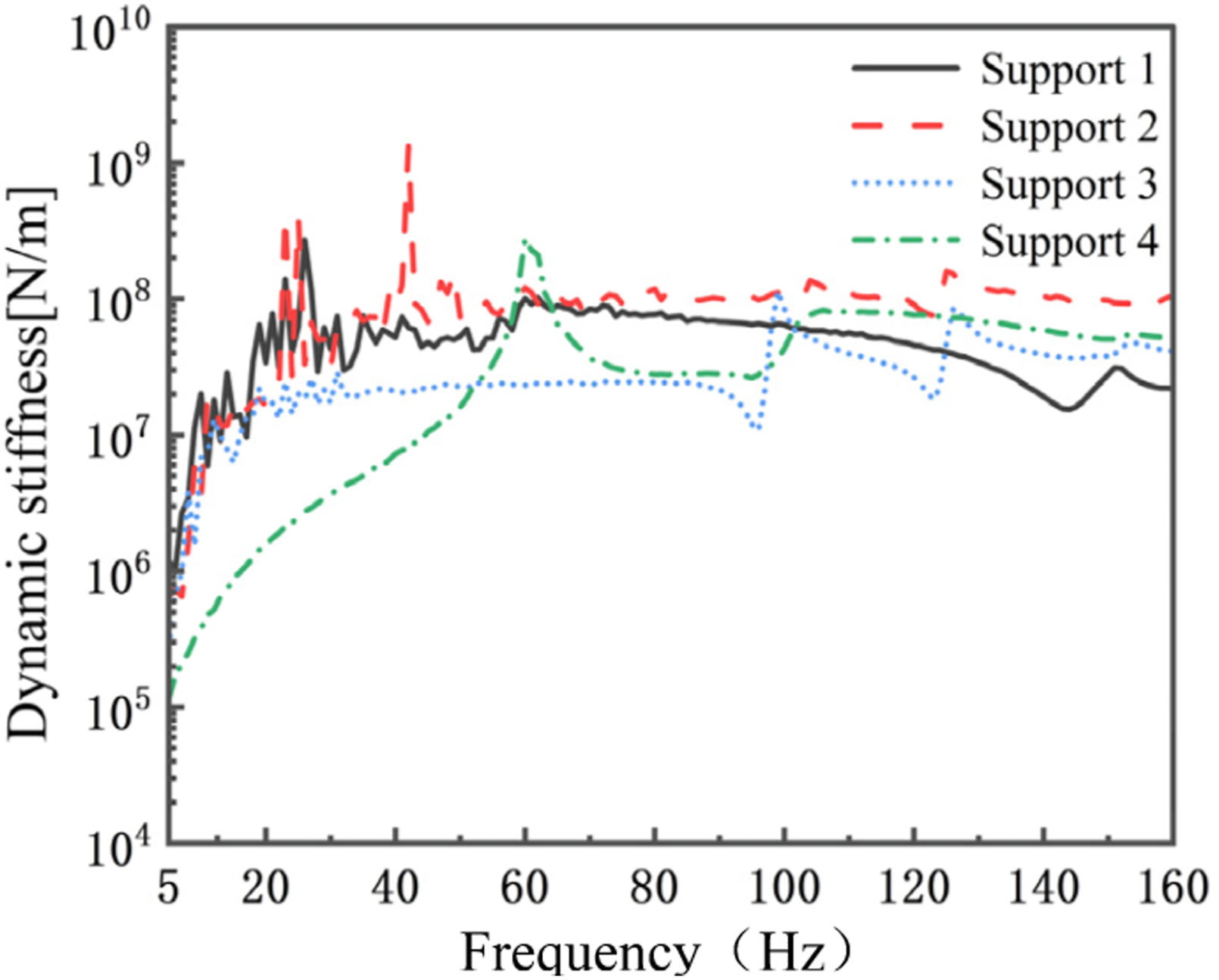
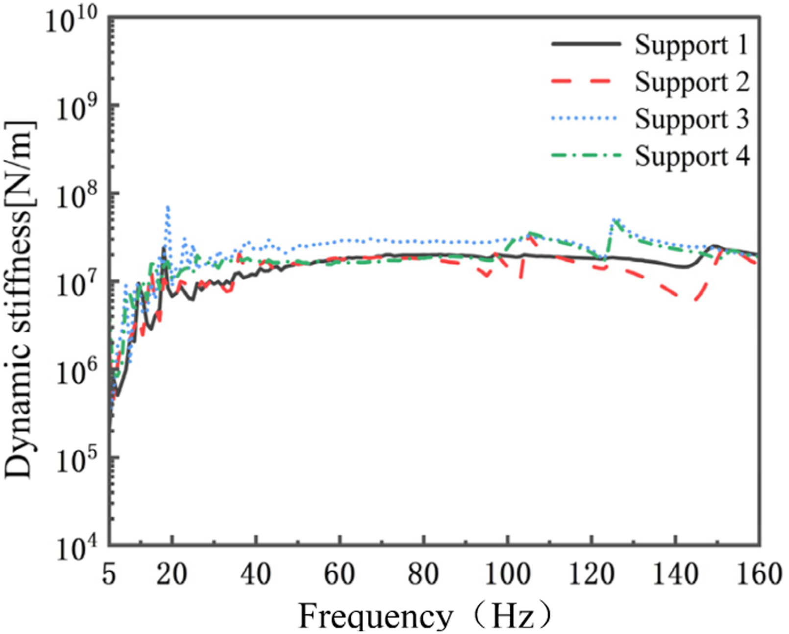
In this work, the dynamic stiffness of pipeline supports is measured in accordance with the standard GB/T 22159-2012, using the direct method to determine the point dynamic stiffness of the pipeline supports. Specifically, this method measures the force applied at the input end of pipeline support and the corresponding vibration acceleration at the same input location. Both the force and acceleration are expressed as complex quantities, from which the point dynamic stiffness at different frequencies is derived: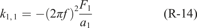
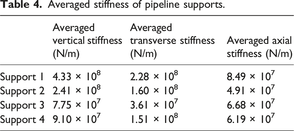
The magnitude of the dynamic stiffness is shown in Figures 15–17. Since it is impossible to use frequency-domain measurement data, the FTDM takes the fixed stiffness as the boundary condition for the pipeline support. The fixed stiffness is determined according to Figures 15–17, and the specific values are shown in Table 4. Dynamic stiffness Dynamic stiffness Dynamic stiffness Averaged stiffness of pipeline supports.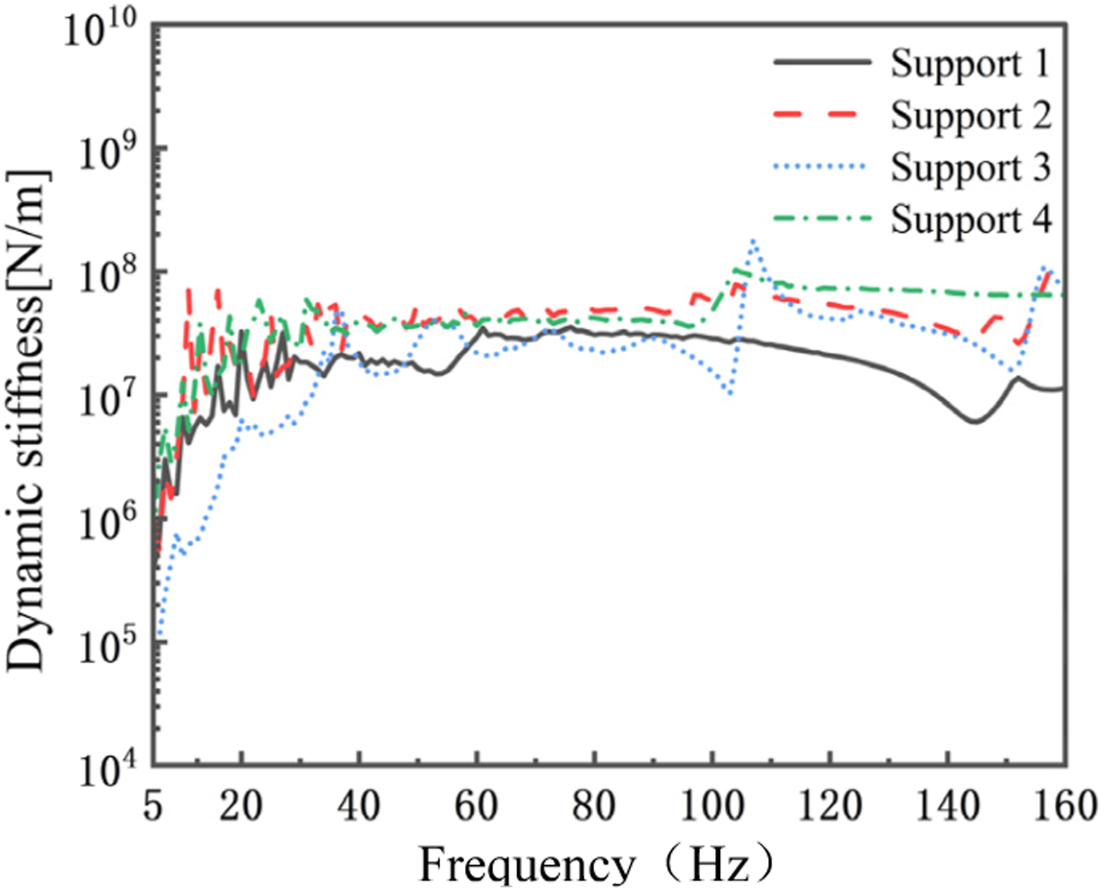
Verification of the numerical model
A harmonic response analysis for the pipeline with a 90° elbow is conducted. A vertical excitation load positioned 100 mm from the upstream of the elbow is implemented. The vibration responses at the measurement points (shown in Figure 2) are measured. Compare the calculational results with the experimental results, as shown in Figure 18. The results calculated by the TFDHM are consistent closely with the experimental results. The peaks and valleys from the results calculated by the FTDM show frequency shifts. This deviation is primarily due to the fixed stiffness used in the FTDM. Harmonic response from numerical calculation and experimental tests in vertical direction: (a) at point A and (b) at point B.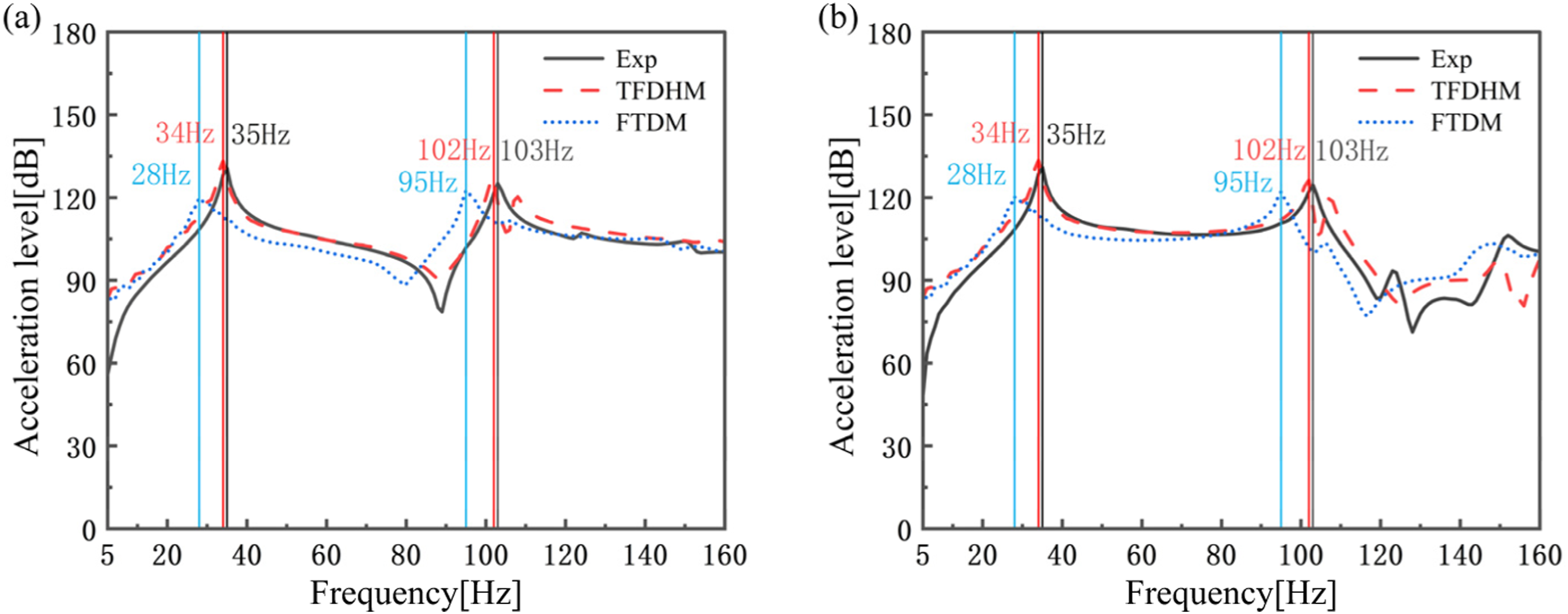
Verification of the vibration calculation
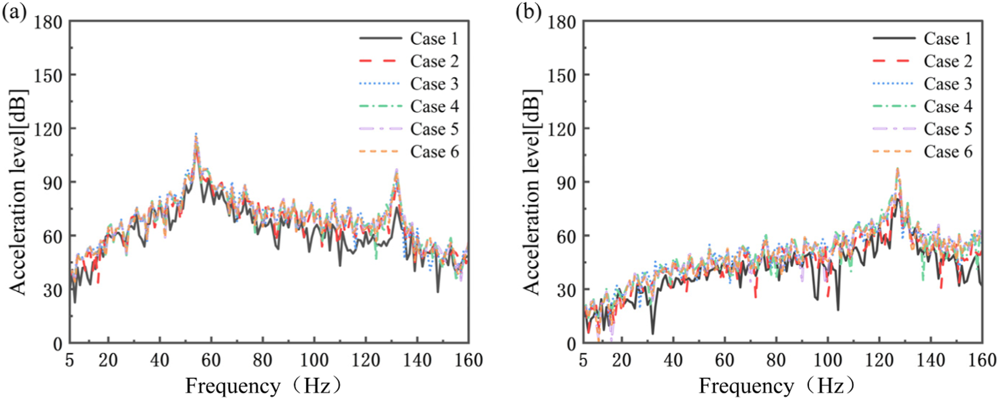
A FIV experiment is conducted on the pipeline with a 90° elbow. In the TFDHM, the fluid load is employed as concluded in Section 3.2.2. The FIV responses at the measurement points (shown in Figure 2) are presented in Figures 19 and 20. Overall, the results calculated by the TFDHM show good consistency with the experimental results. The deviations can primarily be attributed to two factors: (a) The actual pipeline support is a planar constraint. Whereas TFDHM is based on one-dimensional beam elements, which approximate it as a point constraint. (b) The nonlinear damping of the gasket at the flange connection is not included in the computational model, which reduces FIV responses. FIV response from numerical calculation and experimental tests at point A: (a) vertical direction and (b) transverse direction. FIV response from numerical calculation and experimental tests at point B: (a) vertical direction and (b) transverse direction.
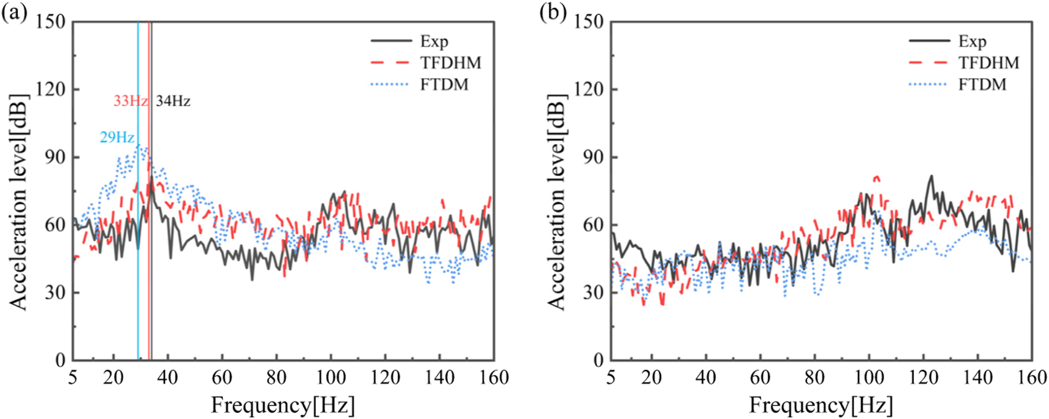
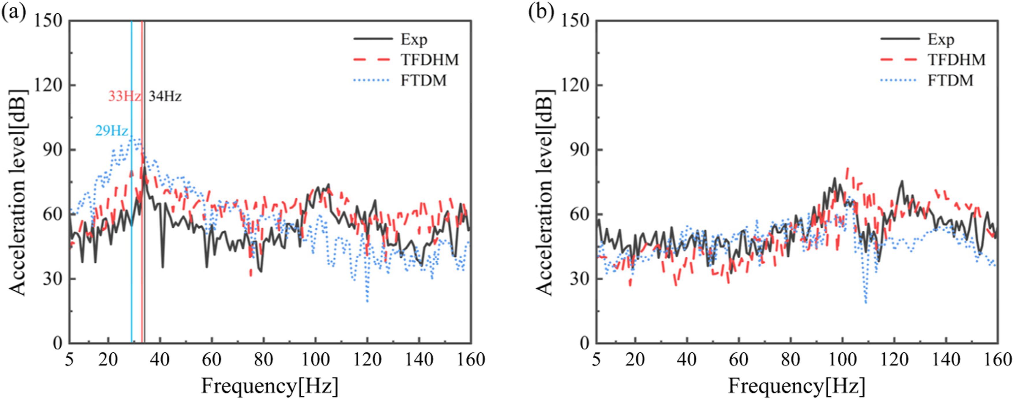
The analysis of the longitudinal FIV responses shows that the results calculated by the TFDHM better match the experimental results. In contrast, the results calculated by the FTDM are higher than the experimental results at low frequencies and lower than the experimental results at high frequencies. For the transverse FIV responses, the TFDHM results align closely with the experimental results, while the FTDM results fall below the experimental data beyond 90 Hz.
Comparison of overall acceleration level by numerical calculation and experimental tests.
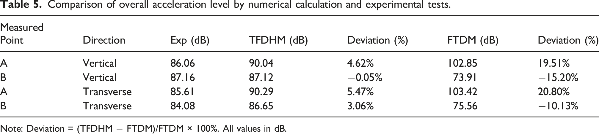
Note: Deviation = (TFDHM − FTDM)/FTDM × 100%. All values in dB.
Conclusion
The TFDHM is developed for the analysis of FIV. The fluid flow is simulated by LES in the time-domain to ensure an accurate solution of the fluctuating pressure acting on the pipeline. The vibration response is solved based on the beam theory using the FEM in the frequency-domain to save the computational time. The FLMM is proposed to convert the 3D time-domain pressure into the frequency-domain point load for application to a beam model. Not only the accuracy, but also numerical performance and engineering practicality of the TFDHM have been verified based on the pipeline with an elbow. (i) The FIV responses calculated by the TFDHM adopting complex excitation loads is consistent closely with those from the FTDM. The solution of the structural response using the TFDHM costs 45 seconds, while it takes 23 hours and 47 minutes using the FTDM. It is indicated that TFDHM maintains accuracy equivalent to that of FTDM while markedly enhancing efficiency through optimized load mapping and geometric simplification. (ii) The pipeline segmentation is one of the key factors on the accuracy of the TFDHM. It is found that insufficient pipeline segmentation can lead to load mapping distortion. The FIV response results trend to converge when the segment count reaches a certain threshold. (iii) Influences of fluid loads on different sections of the pipeline are discussed. In the present cases, the results obtained with fluid loads originating at the elbow and a 2D section upstream and downstream are already acceptable. It means the fluid loads in the pipeline with weak turbulence are negligible for the FIV analysis, which may save computational time. (iv) The FIV experiment is conducted. The TFDHM results show better agreement with the experimental results than the FTDM. This is attributed to the employment of the measured dynamic stiffness of pipeline supports in the frequency-domain, since the TFDHM solved the structural response in the frequency-domain. This indicates that TFDHM has much higher engineering practicality than FTDM.
Footnotes
Funding
The authors disclosed receipt of the following financial support for the research, authorship, and/or publication of this article: This research is supported by the Open Fund Project of Hanjiang National Laboratory (No.KF2024016).
Declaration of conflicting interests
The authors declared no potential conflicts of interest with respect to the research, authorship, and/or publication of this article.