An improved attention mechanism rolling element bearing fault diagnosis based on convolutional neural network and bi-directional long short-term memory

Abstract

In this work, an improved attention mechanism rolling element bearing (REB) fault diagnosis method based on a convolutional neural network (CNN) and a Bi-directional long-short term memory (BiLSTM) is proposed. The original REB fault signals of 10 different fault types are selected from the bearing standard database of Case Western Reserve University (CWRU). The variational mode decomposition optimized by crested porcupine optimizer algorithm (CPO-VMD) is used for pre-processing REB fault signals into multiple intrinsic mode functions (IMF). The Squeeze-and-Excitation (SE) attention is inserted into the convolutional module to adjust the weight relationship between channels, thereby extracting more feature information. After the BiLSTM network structure, self-attention is introduced to focus on important fault characteristics. The experimental results show that the training time of the CNN-SENet-BiLSTM-Self-Attention REB fault diagnosis model proposed in this paper is 39 s, with an accuracy of 99.67%. Compared with the traditional CNN-LSTM, CNN-BiLSTM, CNN-SENet-BiLSTM, CNN-BiLSTM-Self-Attention, and CNN-SENet-LSTM-Self-Attention models, the accuracy rates increase by 9%, 8%, 1.7%, 0.7%, and 0.3%, respectively.

Keywords

rolling element bearings fault diagnosis attention convolutional neural network bi-direction long short-term memory

Introduction

The rolling element bearings (REB) are a crucial component of mechanical systems (Wang et al., 2024); therefore, it is self-evident that REB fault diagnosis is profoundly relevant to the stability and safety of the modern industrial system development (Wang et al., 2022). In REB fault diagnosis, the damage state is determined through the detection, isolation, and identification of data collected by REB health monitoring. Recent years have seen a boom in research regarding the diagnosis and extraction of faults from REB (Qiao et al., 2023). These REB fault diagnosis methods fall under two large synthesis categories: time–frequency domain analysis (Tang et al., 2022) and deep learning-based feature extraction approaches (Chen et al., 2023).

Time-frequency domain analysis is a simple, effective, and stable technique for detecting and diagnosing REB faults (Liu et al., 2024b). Early in the process of mechanical equipment fault diagnosis, simple time–frequency domain signals were used to diagnose the fault. N.E. Huang proposed empirical mode decomposition (EMD), a typical time–frequency domain signal decomposition method that is used for analyzing non-linear and non-stationary signals (Mathur et al., 2023). Meng et al. (2022) selected the time-domain characteristics of REB vibration signals from wind turbines and then added four classifiers to analyze faults. Cui et al. (2021) proposed a fault diagnosis technique for the REB components using maximum correlation kurtosis deconvolution (MCKD) and variational mode decomposition (VMD). However, the main disadvantage is that the results of MCKD are greatly influenced by external noise, and VMD parameters are difficult to select. He et al. (2021) used VMD adaptive morphology in combination with particle swarm optimization algorithms to achieve adaptive filtering and the REB feature extraction. The VMD method demonstrated a more significant advantage over the EMD adaptive morphology method for extracting the characteristic frequency of the fault signal.

Due to advancements in diagnostic technology, the traditional diagnostic method is no longer sufficient to meet the evolving needs. As a result, more reliable and accurate modern REB fault diagnosis methods have been developed, such as deep learning. The core of REB fault diagnosis through deep learning is the identification of fault characteristics and the precision of categorization (Liu et al., 2024a). Various diagnostic approaches exist today that indicate the connection between REB faults and characteristics, including decision trees (Alhams et al., 2024), support vector machines (Fu et al., 2023), K-Nearest Neighbors (Khawaja et al., 2024), and artificial neural networks (Yang et al., 2025). Consequently, these diagnostic techniques can autonomously identify REB fault characteristics with significant diagnostic precision (Khorram et al., 2021; Zhou et al., 2024). Khorram et al. (2021) proposed a recurrent neural network model according to the convolutional LSTM, revealing high detection accuracy and strong feasibility. Skowron et al. (2024) provided an alternative to the well-known classical diagnostic tools based on advanced signal processing methods based on convolutional neural networks (CNN) and Hilbert-Huang transform (HHT). The proposed method achieved a classification accuracy of 99.8% on the test set. Zhou et al. (2024) proposed a REB fault diagnosis method based on EEMD and LSTM to extract fault features automatically and achieved a good fault diagnosis result. Despite all the advantages of the aforementioned methods, they still suffer from shortcomings in the complete extraction of contextual feature information of the sequence signal (Shang et al., 2025). In addition to the deep learning-based approaches mentioned above, there is another line of research focused on enhancing weak fault characteristics under noisy conditions through signal processing techniques such as stochastic resonance (SR). For instance, the stochastic resonance array (SRA) method designs noise-boosted filter banks to amplify multi-harmonic fault features. Similarly, studies on fractional nonlinear systems demonstrate that widening the potential well can improve weak signal detection in mechanical fault diagnosis (Zhou et al., 2025). While these methods excel in extracting sub-harmonic and weak periodic components, they often serve as pre-processing steps and require careful parameter tuning (Ma et al., 2022). In contrast, our proposed model integrates adaptive attention mechanisms (SENet and Self-Attention) within a deep learning framework to dynamically highlight fault-related features and suppress noise interference, enabling end-to-end fault diagnosis without explicit noise injection or manual feature engineering. This makes our approach more suitable for automated industrial applications where operational conditions vary widely.

The study aims to improve the CNN and BiLSTM network performance using SENet attention and the Self-Attention mechanism to implement high-precision intelligent diagnosis of REB faults. Meanwhile, the VMD method based on the crested porcupine optimizer (CPO) was applied to REB signal preprocessing. The proposed model can easily fit various datasets by utilizing contextual information to improve detection accuracy, which offers a crucial guideline for detecting REB faults in real-world variable working conditions in engineering.

Methodology

This study uses the CWRU REB standard database to explore a deep learning-based approach for analyzing bearing faults. An improved attention mechanism for rolling element bearing fault diagnosis based on CNN-BiLSTM is proposed. The time-domain features of distinct bearing defect signals are examined, which provides the preprocessing parameters for the subsequent analysis of bearing fault detection accuracy through the proposed model.

Time–frequency domain feature analysis

The time–frequency domain analysis method is a kind of preprocessing method for bearing fault original vibration signal directly, which can provide some evidence for the traditional bearing fault diagnosis. Analysis of fault time-domain characteristics of different bearings is performed by calculating dimensional and dimensionless parameters. The parameters, such as mean value, peak, root mean square, skewness, root amplitude, and kurtosis, are extracted as the dimensional characteristics. The parameters, such as kurtosis factor, peak factor, shape factor, Impulse factor, and clearance factor, are extracted as dimensionless characteristics.

Signal preprocessing

This section of signal preprocessing is divided into three stages. The first stage of signal preprocessing: CPO optimizer is used as an optimization function to improve the VMD decomposition performance. The second stage of signal preprocessing: Selecting the minimum permutation entropy as the fitness function for algorithm optimization. The third stage of signal preprocessing: Calculating the IMF components as a feature vector.

Crested porcupine optimizer algorithm

In order to achieve the best decomposition effect, highlight the characteristic frequencies of bearing faults, and improve the accuracy of fault diagnosis, a CPO was employed to optimize the VMD parameters (Salas et al., 2024). The VMD optimization algorithm based on the CPO is proposed to address the issues of mode mixing and high noise content in the processing of bearing vibration signals using EMD and EEMD. This algorithm uses the minimum permutation entropy as the fitness function, iteratively updates the optimal number of decomposition modes and penalty factors using the global search capability of the CPO algorithm, and then reconstructs the bearing vibration signal into multiple intrinsic mode function (IMF) components through VMD to extract its fault characteristic frequency. During the CPO optimization of VMD, each time CPO conducts an iterative search, it will calculate a fitness function value (or referred to as the minimum permutation entropy) and calculate the fitness function value for each IMF component.

The minimum permutation entropy

In the optimization process, select the minimum permutation entropy as the fitness function to calculate the fitness function values of each IMF component. This article analyzes the fitness function curve and obtains the optimal parameter K and a, so as to obtain the optimal decomposition curve of VMD.

Permutation entropy characterizes the dynamic behavior of a system by mapping continuous time-domain signals into a sequence of symbols. Permutation entropy has the advantages of simple calculation, fast speed, and strong noise resistance, which is often used for mechanical fault diagnosis and medical electrocardiogram signal analysis. Assuming that the REB time series is X (i) = {x₁, x₂, … x_n,}, which is rebuilt as:

X (i) = {x (1), x (1 + τ), \dots, x [1 + (m - 1) τ]}

(1)

X (N - (m - 1) τ) = {x (N - (m - 1) τ), x (N - (m - 2) τ), . . ., x (N)}

(2)

Here, m is the embedding dimension and τ is the time delay.

For example, when m = 3, τ = 2, sorting the time series X {10, 30, 20}, which can be written as (1, 3, 2). When m = 2, there are only two possible directions from position x₁ to x₂: up and down; When m = 3, x₃ may have three different positional distributions. Finally, a total of m factorial different sequential patterns are generated.

Therefore, the probability of each sorting occurring is as follows:

P (i) = \frac{N u m (X (i))}{N - (m - 1) x}

(3)

Permutation entropy can be calculated based on information entropy:

H_{P E} (m) = - \sum_{π = 1}^{π = m!} P (π) \ln (P (π))

(4)

Here, m = 3, τ = 1. By the above calculation process, we can detect changes in bearing signals, where a lower entropy value indicates a more regular time series.

Feature vector

The CPO-VMD is used for pre-processing REB fault signals into IMFs. The IMF components as reconstructed fault signal for REB are used to calculate the eigenvalues of nine-dimensional and non-dimensional parameters. Nine feature parameters are selected to compose a feature vector that can characterize the bearing state. The feature vectors composed of the selected 10 fault types are used as training and testing sets, which are placed into the model proposed in this article.

CNN and BiLSTM with improved attention mechanism

Convolution neural network

CNN is a deep feedforward neural network with local connections and weight sharing. CNN is mainly used for processing time series data, which extracts features by performing one-dimensional convolution operations on the input data. 1D-CNN can be well combined with BiLSTM by capturing local patterns and sequential information. The basic structure of 1D-CNN generally includes: convolution layers, activation functions, pooling layers, fully connected layers, and output layers (Deng et al., 2025).

Bidirectional long short-term memory

LSTM, a special RNN structure, is used for processing and learning time series data (Sun and Zhao, 2021). LSTM can better capture and utilize long-term dependencies in time series data by introducing a gating unit mechanism, thereby improving the performance and generalization ability of the model. Compared to LSTM, BiLSTM can better capture contextual information and improve model accuracy when processing sequential data (Tong et al., 2022). BiLSTM models can enhance the robustness and generalization capability of a model by leveraging contextual information to extract improved feature representations.

Improved attention mechanism

An attention mechanism is a data processing method that is used to continuously monitor a key location in deep learning. The attention mechanism’s level of attention to different information is reflected by weights (Ding et al., 2024). The attention mechanism can be viewed as a query, key, and weighted average, forming a multilayer perceptron (Zou et al., 2024).

The Squeeze-and-Excitation networks (SENet) are a kind of channel attention mechanism (Ye et al., 2024). The core operations of SENet can be summarized into three steps. Firstly, the squeeze operation: Using spatial dimension for feature compression, and converting each feature channel into a real number. Then, excitation operation: Using parameter w to regenerate weights for each feature channel. Last, reweight operation: Weighted channel by channel through multiplication onto previous features.

The Self-Attention mechanism calculates the response of each position in the sequence by focusing on all positions in the same sequence (Ullah et al., 2024). Compared to the attention mechanism, the Self-Attention mechanism’s query and key are derived from the same set of elements. The formula for calculating Attention in the form of key-value pairs is as follows:

a t t (Q, K, V) = S o f t \max (\frac{f (Q, K^{T})}{\sqrt{d_{k}}}) V

(5)

Here, Q, K, and V represent the query value, calculated value, and weight respectively. d_k is the eigenvector dimension.

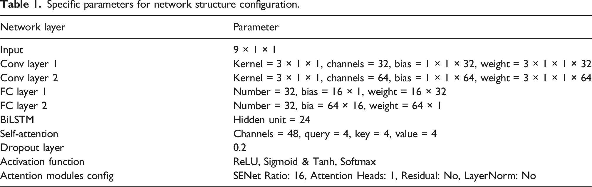
In this study, the reduction ratio of the SENet module is set to 16. A single-head Self-Attention mechanism (Head = 1) is employed in this work. For the sake of model simplicity and parameter efficiency, residual connections and layer normalization are not used in conjunction with the Self-Attention module. The selection of these hyperparameters has also been integrated into the overall network architecture table (Table 1) to provide a comprehensive overview.

Table 1.

Specific parameters for network structure configuration.

Network layer	Parameter
Input	9 × 1 × 1
Conv layer 1	Kernel = 3 × 1 × 1, channels = 32, bias = 1 × 1 × 32, weight = 3 × 1 × 1 × 32
Conv layer 2	Kernel = 3 × 1 × 1, channels = 64, bias = 1 × 1 × 64, weight = 3 × 1 × 1 × 64
FC layer 1	Number = 32, bias = 16 × 1, weight = 16 × 32
FC layer 2	Number = 32, bia = 64 × 16, weight = 64 × 1
BiLSTM	Hidden unit = 24
Self-attention	Channels = 48, query = 4, key = 4, value = 4
Dropout layer	0.2
Activation function	ReLU, Sigmoid & Tanh, Softmax
Attention modules config	SENet Ratio: 16, Attention Heads: 1, Residual: No, LayerNorm: No

CNN-SENet-BiLSTM-self-attention model

This article proposed the combination of SENet and Self-Attention attention mechanisms with a CNN-BiLSTM neural network. SENet is inserted into the convolution module to adjust the weight relationship between the convolutional channels, thereby extracting more bearing feature information. Meanwhile, after the BiLSTM network structure, Self-Attention is introduced to focus on its more important features in long sequences.

As shown in Figure 1, the convolutional layers and activation functions in CNN together form a convolutional block. The bearing sequence first undergoes a bearing fault feature extraction operation through the CNN convolutional block, and outputs a feature map. Through the SENet layer, composed of global average pooling and fully connected layers, compression and excitation operations are performed to enhance the features. Then, the feature sequence is unfolded and input into the BiLSTM network structure. BiLSTM processes the input sequence in both forward and backward directions to obtain the forward state hidden sequence and the backward state hidden sequence. Using the output of the BiLSTM layer as the input of the Self-Attention layer, key features are highlighted by reallocating attention weights in the Self-Attention layer, and finally output through a fully connected layer and classification function.

Figure 1.

The flowchart of the CNN-SENet-BiLSTM-Self-Attention model.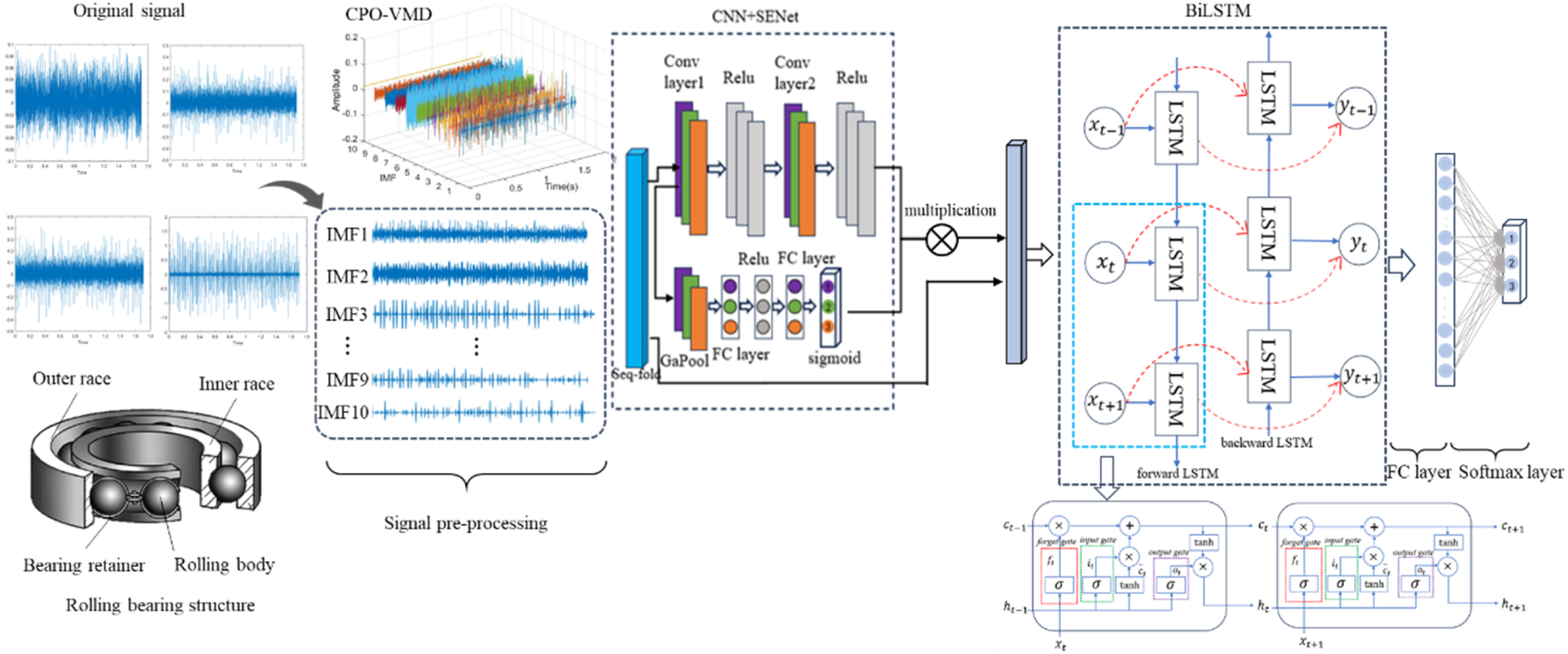

The bearing fault diagnosis method based on CNN-SENet-BiLSTM-Self-Attention is first based on signal preprocessing. The VMD method optimized by a genetic algorithm is used to decompose and reconstruct the bearing vibration signal. The decomposed IMF component is used to obtain the time-domain characteristic parameter values, and the calculated time-domain characteristic parameter values are used to form the characteristic vector. Subsequently, input the feature vectors into the CNN-SENet-BiLSTM-Self-Attention model to partition the dataset. Following this, set parameters such as learning rate, optimizer, and iteration count to train the network model. Use the test set data to test the performance of the training model, and finally, output the diagnostic results of fault classification through softmax. The diagnostic process is shown in Figure 2 below:

Figure 2.

Flow chart for bearing fault diagnosis.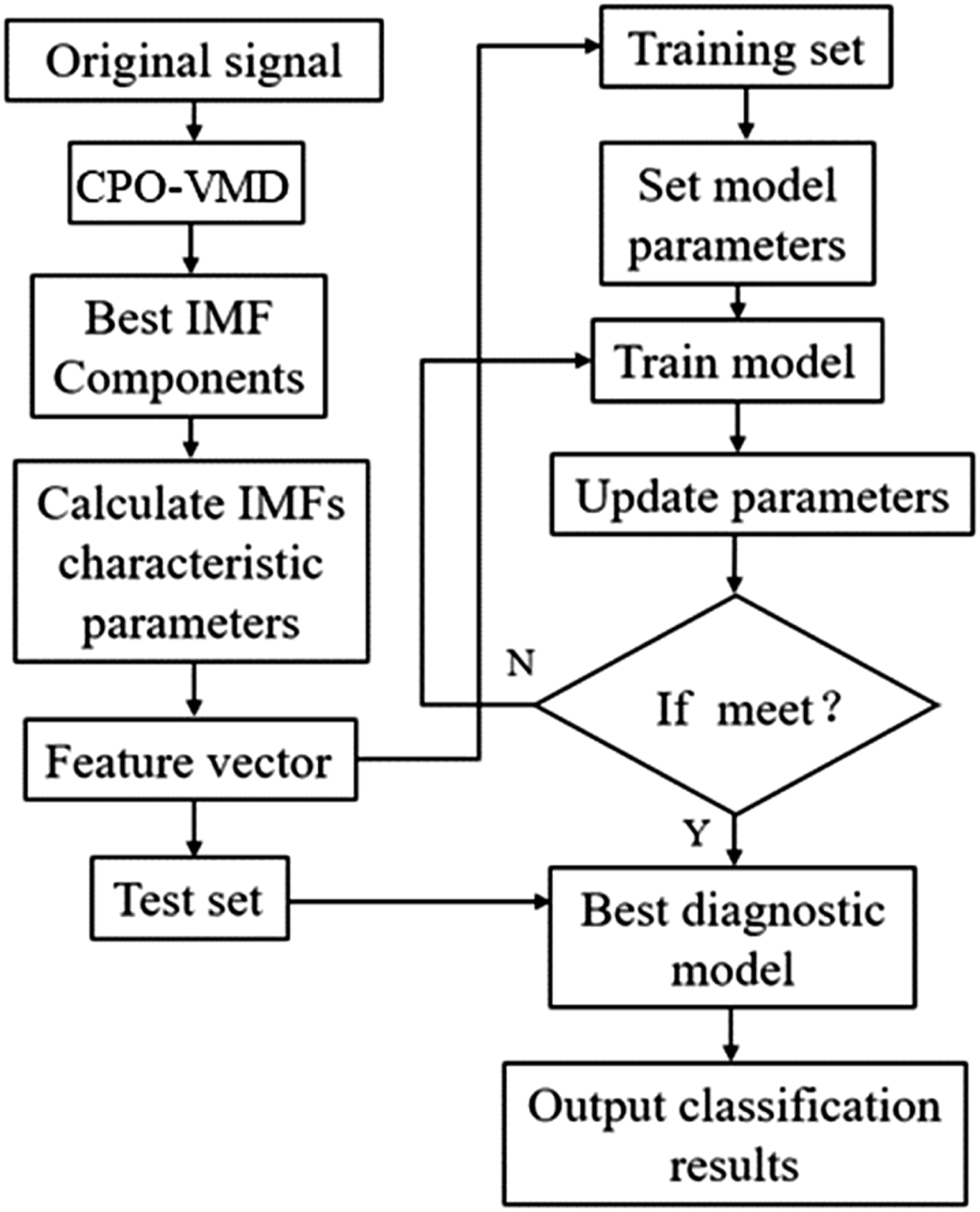

The detailed parameter configuration of the proposed network is summarized in Table 1.

Experimental data and parameter selection

This experiment selected the CWRU bearing data center with a speed of 1772 rpm, motor load of 1 Hp, and acceleration data at the bearing drive end. Data of inner ring faults, outer ring faults, rolling element faults, and normal bearing were extracted respectively, with fault depths of 0.007 inches, 0.014 inches, and 0.021 inches, respectively, for signal processing and analysis. After obtaining their feature vectors, divide the feature vectors into datasets. To fully reflect the characteristics of bearing signals, 12,000 sample points were taken for each type of bearing signal, with a sampling rate of 12,000 Hz. Each category was divided into 300 sample data points, for a total of 3000 samples. Among them, 90% of the training set samples are removed, totaling 2700. The test set samples are reduced by 10%, totaling 300. To facilitate distinction, all bearing faults were labeled. The normal bearing is marked as No. 1. The three types of inner ring faulty bearings with depths of 0.007 inch, 0.014 inch and 0.028 inch are labeled as No. 2, No. 5, and No. 8, respectively. The three types of rolling body faulty bearings with depths of 0.007 inch, 0.014 inch, and 0.028 inch are labeled as No. 3, No. 6, and No. 9, respectively. The three types of outer race faulty bearings with depths of 0.007 inch, 0.014 inch and 0.028 inch are labeled as No. 4, No. 7, and No. 10, respectively.

During the training process, the Adam optimizer was used for training optimization, with 200 rounds of training, 7 iterations per round, and a maximum of 1400 iterations. The initial learning rate is set to 0.01, and when the number of iterations exceeds half, the learning rate is automatically adjusted to 0.0001.

Results and discussion

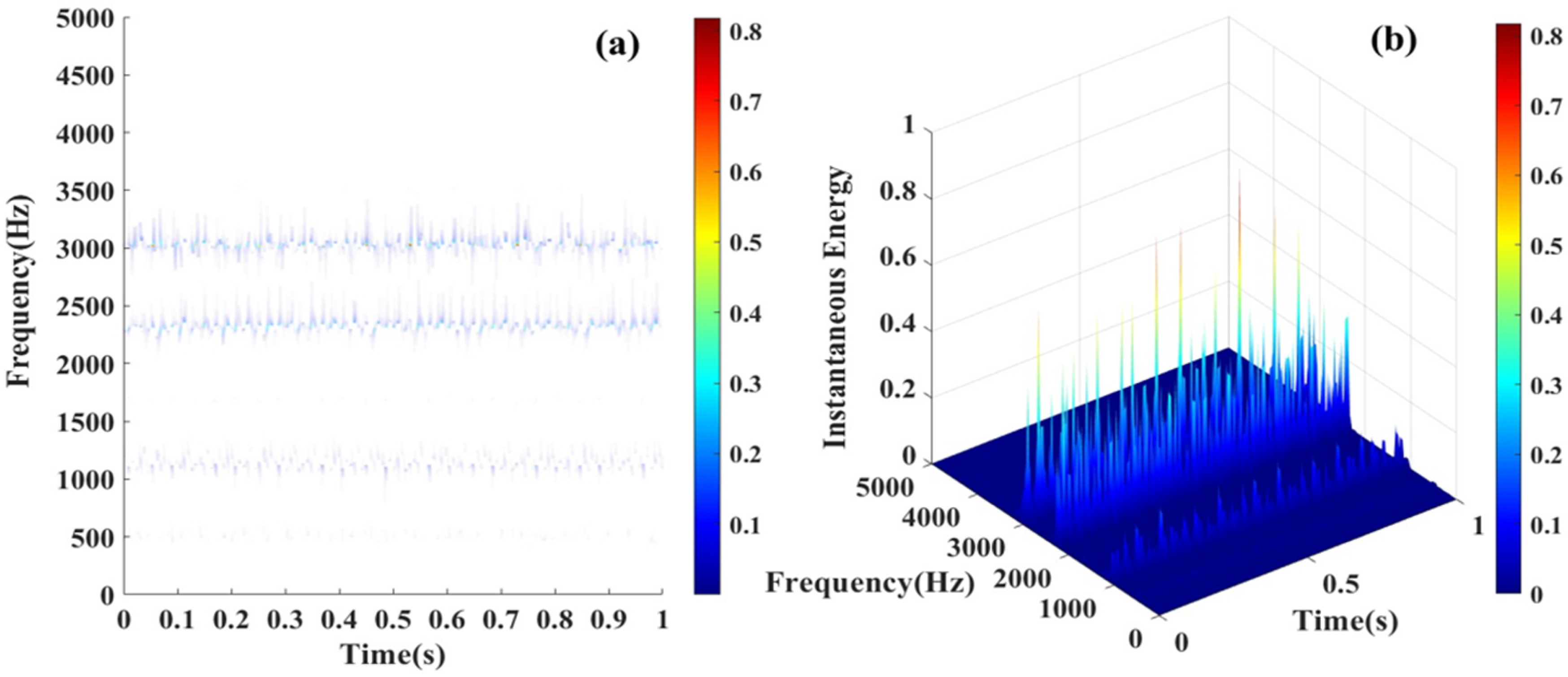
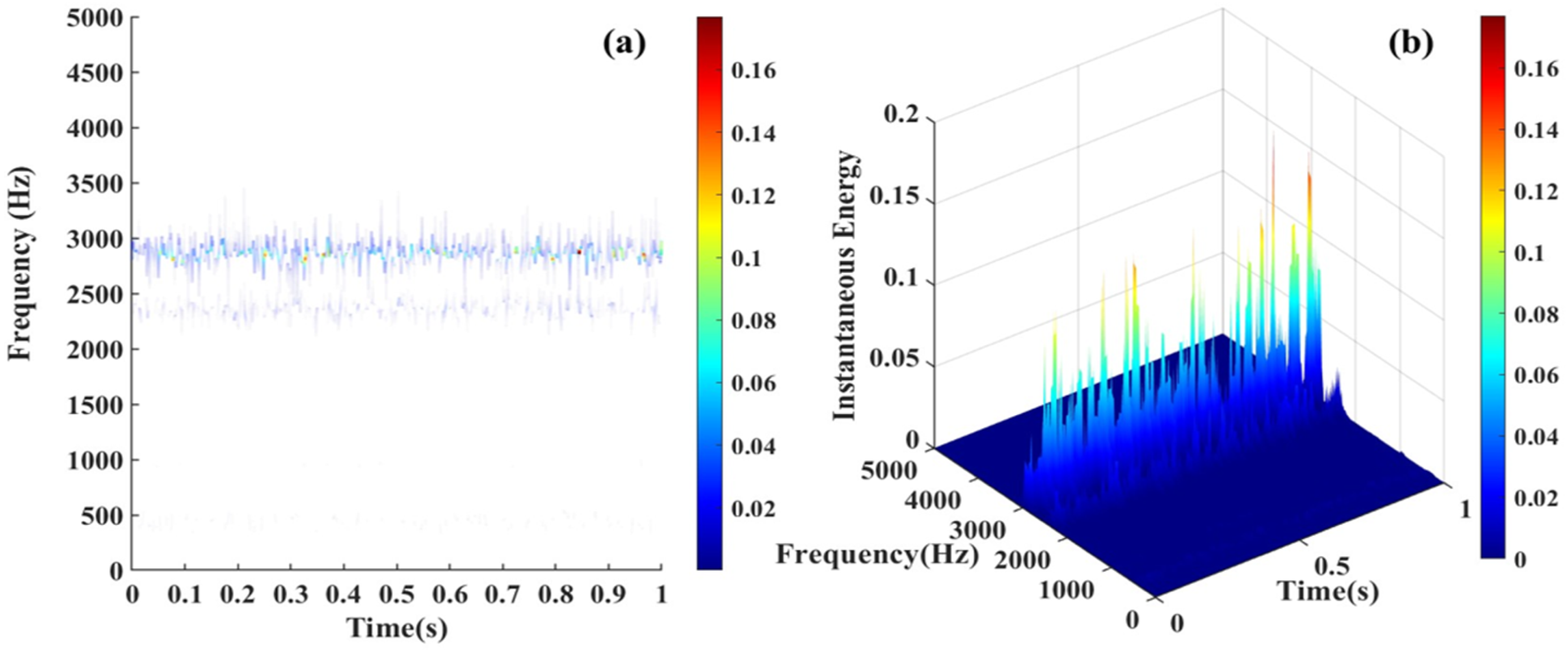
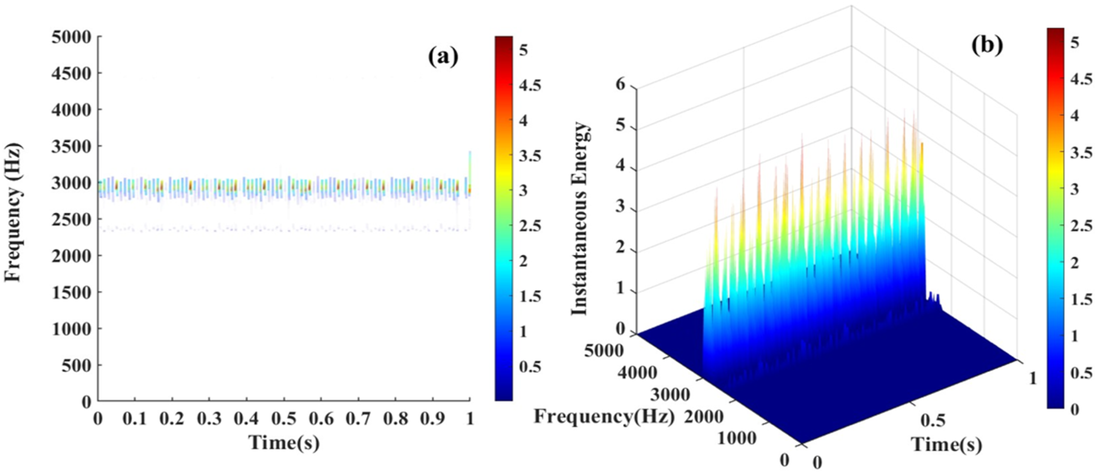
From Figures 3–6(a) represent the main frequency distribution of four different types of bearing fault signals in different frequency ranges. Among them, the main frequency of normal bearing signals is mainly distributed in the low frequency range of 100–200 Hz, while the main frequency and harmonics of bearing inner ring fault signals, outer ring fault signals, and rolling element fault signals are mostly distributed in the mid to high frequency range of around 3000 Hz, with only differences in energy changes. Figures 3–6(b) are mainly used to observe the instantaneous energy levels of each frequency band spectrum. As shown in Figure 6(b), compared with normal bearing signals, inner ring faults, and rolling element faults, the instantaneous frequency spectrum energy of the outer ring fault signal has increased by several energy levels. The instantaneous energy spectrum of the outer ring fault signal can reach up to 5 V square, and the energy spectrum shows a sawtooth shape. This is because the outer ring of the bearing has the largest contact surface. When the outer ring fails, it is usually subjected to continuous external force impact, resulting in periodic sawtooth-shaped high-energy spectra. The areas where the energy suddenly increases or decreases also correspond to the instantaneous characteristic changes of the signal.

Figure 3.

Time–frequency domain analysis of REB signals. (a) 2D Hilbert spectrum of normal bearing, (b) 3D Hilbert spectrum of normal bearing.

Figure 4.

Time–frequency domain analysis of REB signals. (a) 2D Hilbert spectrum of inner race fault bearing with 0.007 inch fault depth, (b) 3D Hilbert spectrum of inner race fault bearing with 0.007 inch fault depth.

Figure 5.

Time–frequency domain analysis of REB signals. (a) 2D Hilbert spectrum of rolling body fault bearing with 0.007 inch fault depth, (b) 3D Hilbert spectrum of rolling body fault bearing with 0.007 inch fault depth.

Figure 6.

Time–frequency domain analysis of REB signals. (a) 2D Hilbert spectrum of outer race fault bearing with 0.007-inch fault depth, (b) 3D Hilbert spectrum of outer race fault bearing with 0.007-inch fault depth.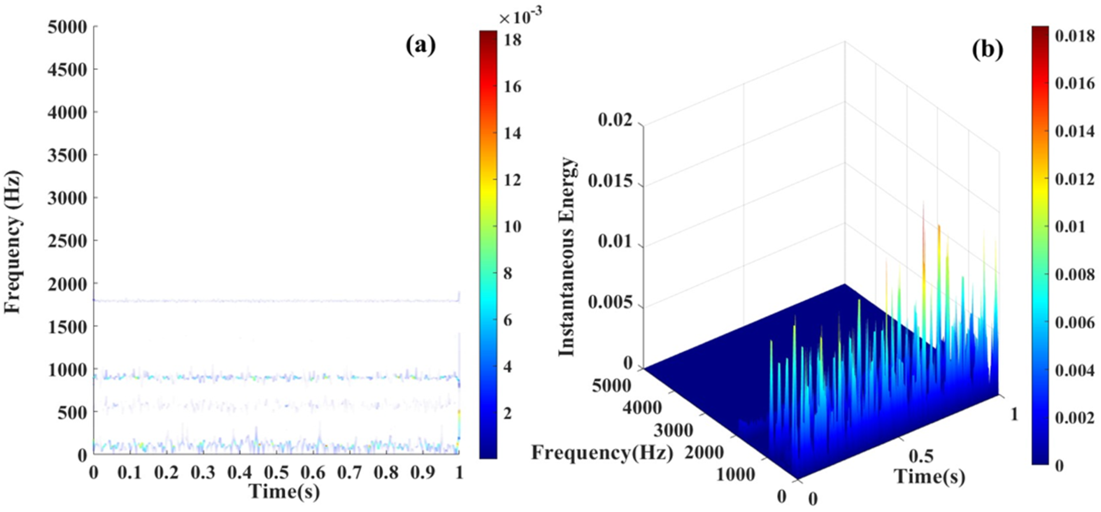

Calculating the dimensional and non-dimensional parameters of the optimal IMF components as feature vectors and building a data set (including test data, train data, and validation data). The data set is put into six models to train. These models output the diagnosis result of the fault prediction and classification.

The output results of the bearing fault diagnosis model based on CNN-SENet-BiLSTM-Self-Attention are shown in Figure 7. The horizontal axis of the confusion matrix corresponds to the 10 fault labels in Table 2, and the vertical axis represents the diagnostic results of the current label. From Figures 3 –6, it can be seen that the accuracy of the bearing fault diagnosis method based on CNN-SENet-BiLSTM-Self-Attention has reached 99.67%. The red square represents the error that occurred, and a normal bearing sample label is diagnosed as a rolling element bearing with a fault of 0.007 inches.

Figure 7.

Classification results of CNN-SENet-BiLSTM-Self-Attention model.

Table 2.

Comparative experiment.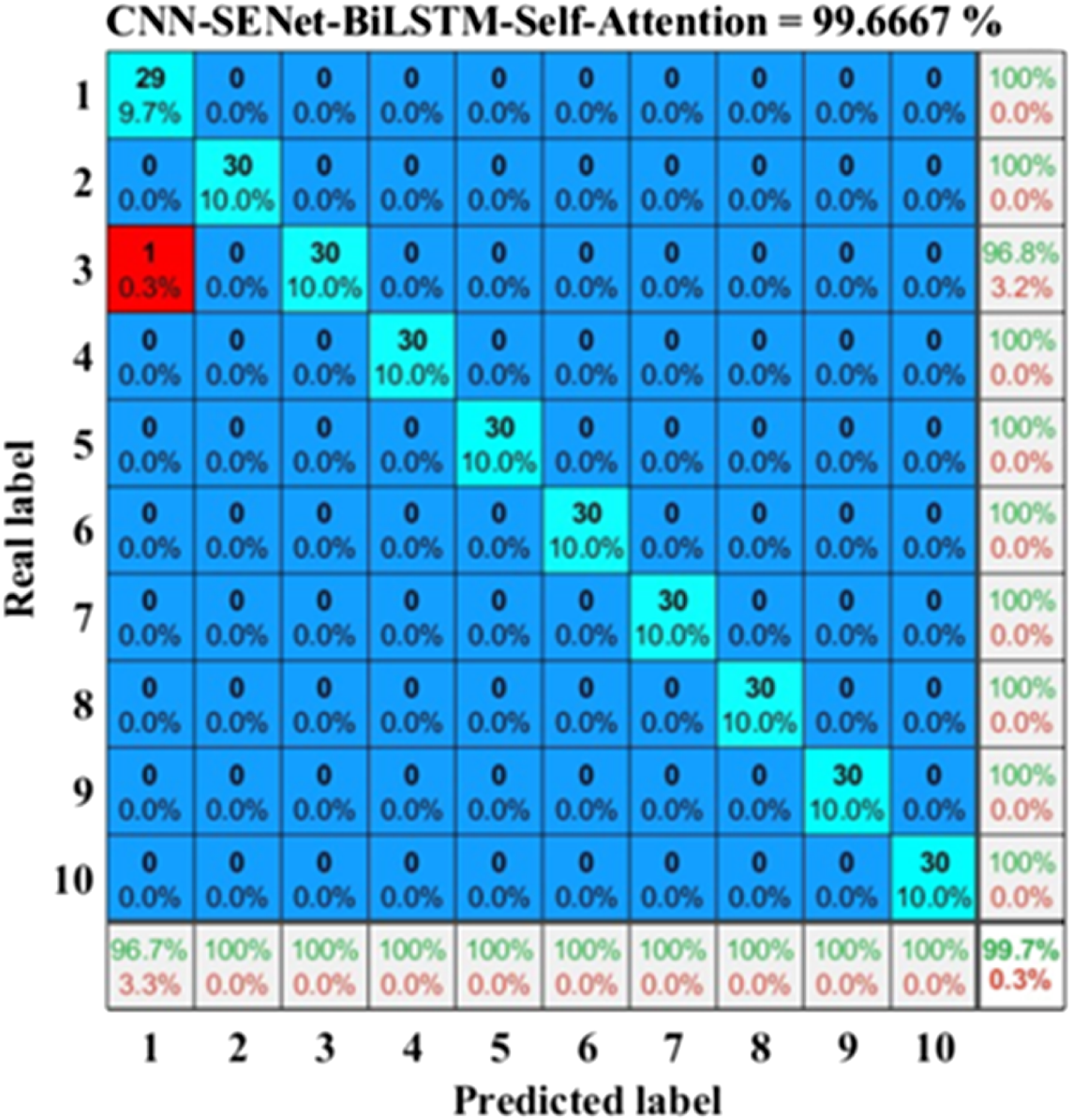

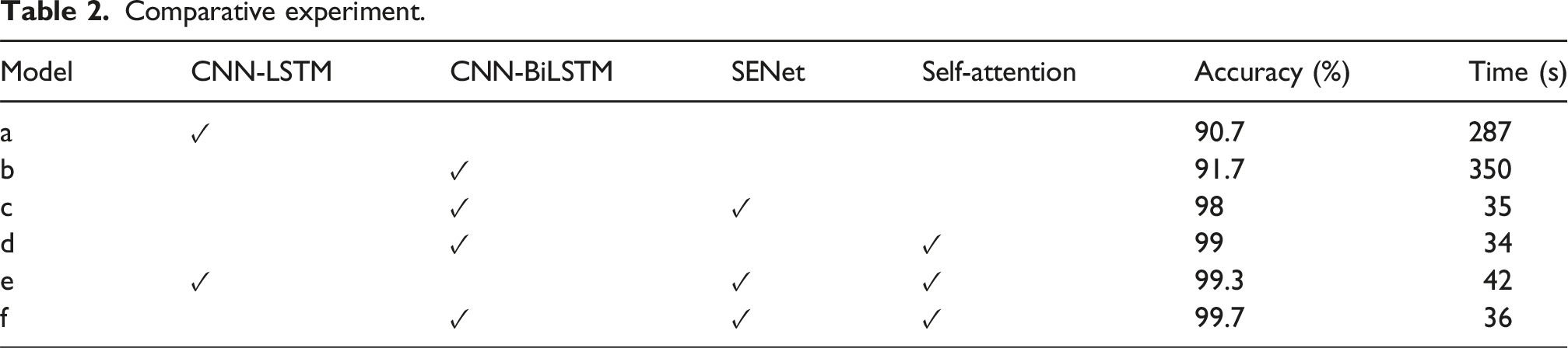
Model	CNN-LSTM	CNN-BiLSTM	SENet	Self-attention	Accuracy (%)	Time (s)
a	✓				90.7	287
b		✓			91.7	350
c		✓	✓		98	35
d		✓		✓	99	34
e	✓		✓	✓	99.3	42
f		✓	✓	✓	99.7	36

Figure 8 shows the visual classification of the model’s fault diagnosis results. These 300 sample numbers together constitute the test set samples for 10 types of bearing faults. The green circle represents the actual fault type, and the blue square represents the predicted fault type.

Figure 8.

Visual classification.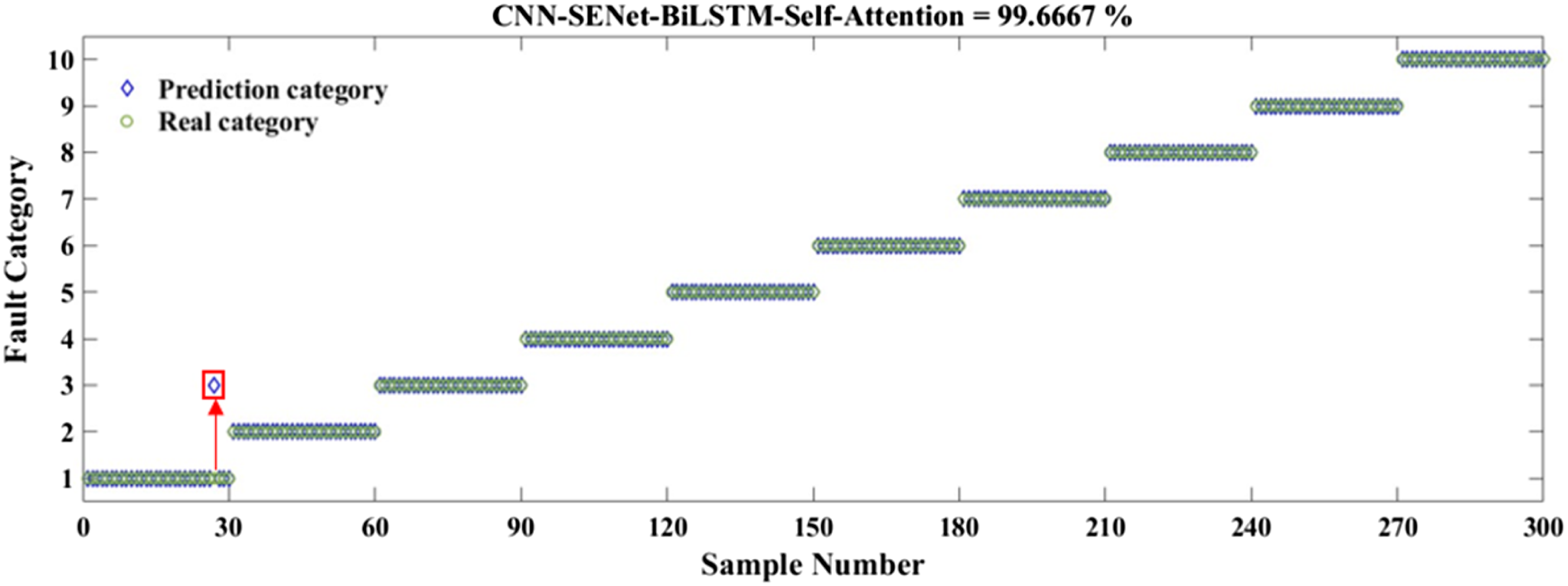

Accuracy and loss function are important indicators for evaluating the quality of a network model. Among them, the higher the accuracy, the better the bearing fault diagnosis effect of the model, while the lower the loss rate, the higher the information utilization efficiency of the model. The diagnostic accuracy and loss function iteration images based on CNN-SENet-BiLSTM-Self-Attention are shown in Figure 9. During the first 200 iterations, the accuracy rapidly increases, and after 200 iterations, the accuracy tends to plateau, reaching over 99% accuracy. Figure 9(b) shows the loss function curve of the model. It can be observed from the graph that the loss function of the model converges quickly in the first 400 iterations, but after 400 iterations, the loss rate gradually becomes flat and finally freezes around 0.1.

Figure 9.

Experimental results of bearing fault diagnosis using CNN-SENet-BiLSTM-Self-Attention model. (a) Accuracy curve, (b) loss function curve.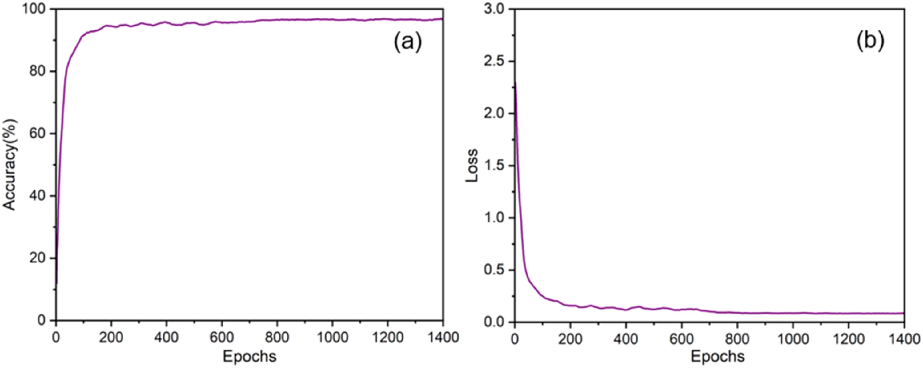

This comparative experiment mainly verifies the CNN + SENet and BiLSTM + Self-Attention structures used in this section. Using CNN-LSTM as the backbone network, validate the CNN-BiLSTM model, CNN-SENet-BiLSTM model, CNN-BiLSTM-Self-Attention model, CNN-SENet-LSTM-Self-Attention model, and CNN-SENet-BiLSTM-Self-Attention model. And evaluated on the CWRU bearing dataset, the experimental results are shown in Figures 10 –12.

Figure 10.

Confusion matrix. (a) CNN-LSTM model; (b) CNN-BiLSTM model.

Figure 11.

Confusion matrix. (a) CNN-SENet-BiLSTM model; (b) CNN-BiLSTM-Self-Attention model.

Figure 12.

Confusion matrix. (a) CNN-SENet-LSTM-Self-Attention model; (b) CNN-SENet-BiLSTM-Self-Attention model.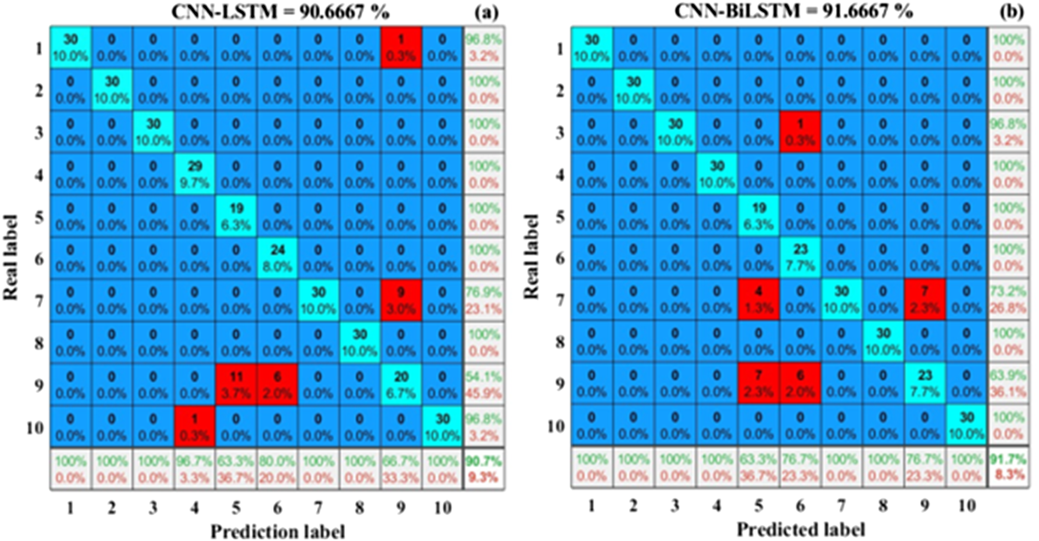

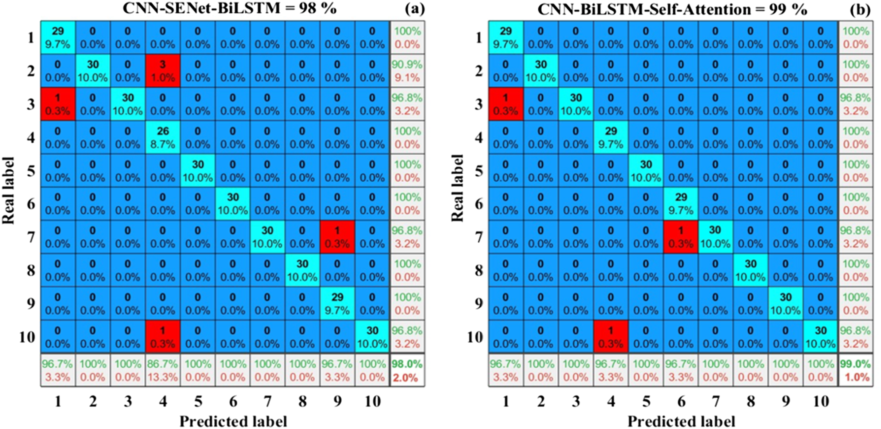
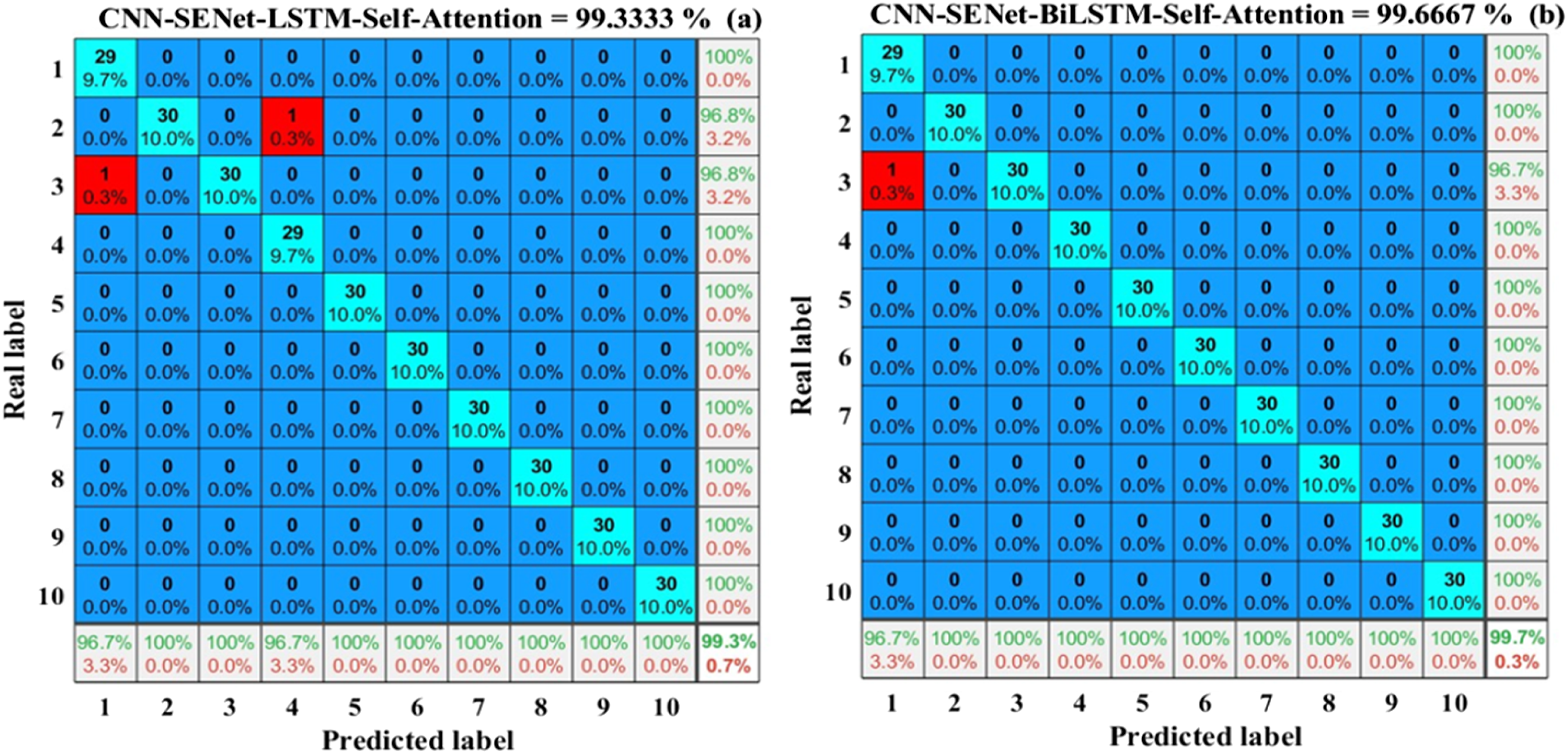
According to Figures 10 –12, these six models are referred to as Model a, Model b, Model c, Model d, Model e, and Model f. Compared to model A, model B improves on LSTM by using BiLSTM. Based on Model B, SENet and Self-Attention structures are respectively adopted to form Model C and Model D. Based on retaining module C or module D, Model F adds Self-Attention or SENet structures respectively. The results of the ablation experiment are shown in Table 2.

By comparing model A and model B, it can be seen that without considering testing time, introducing BiLSTM based on LSTM improves the accuracy of model fault diagnosis by 1%, indicating that BiLSTM can simultaneously capture the information before and after the sequence, which helps enhance feature expression ability. Comparing model f and model b, it can be seen that the fusion attention mechanism proposed in this paper improves the accuracy of bearing fault diagnosis by 8%, reflecting the significant enhancement effect of SENet and Self-Attention attention mechanisms on the performance of the network model. In the selection of the SENet module, by comparing model b and model c, it can be seen that the accuracy has been improved by 6.3%. However, in the selection of the Self-Attention module, it can be seen from the comparison between model b and model c that the accuracy has been improved by 7.3%. This indicates that the SENet module and the Self-Attention module exhibit different enhancement effects when combined into different network structures.

The accuracy of bearing fault diagnosis and the iterative graph of loss function for these six network models are shown in Figure 13. In Figure 13(a), it can be seen that the CNN-SENet-BiLSTM Self-Attention model has the highest final accuracy, reaching up to 99.67%. From Figure 13(b), it can be seen that the CNN-SENet-BiLSTM Self-Attention model has the fastest convergence speed of the loss function, which has basically converged after about 200 iterations, and the minimum loss function value can reach 0.1. This indicates that the CNN-BiLSTM model based on a fusion attention mechanism can effectively achieve bearing fault diagnosis.

Figure 13.

Experimental results of six diagnostic models. (a) The accuracy iteration curves of six models; (b) Iterative curves of loss functions for six models.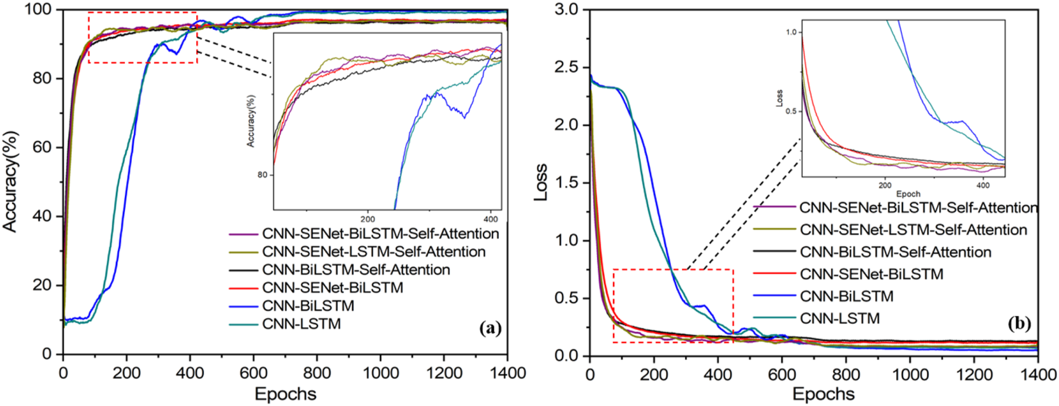

Although the proposed model achieved promising results on the CWRU dataset, we are aware of its limitations and broader challenges in real-world applications.

The generalization capability of the CWRU dataset remains a critical issue requiring further investigation. While our current results are positive, we exercise caution against overstatement. Our selection of the architecture (SENet and Self-Attention) was driven by the expectation of enhanced robustness against noise and operational variations. We believe this provides an initial foundation for generalization capability, which we plan to comprehensively evaluate through cross-condition and cross-domain validation in future work.

The journey from laboratory validation to field deployment remains long. This study represents an exploratory effort demonstrating the method’s potential in controlled settings. The mechanisms introduced aim to address practical challenges such as noise. As a natural next step, we intend to conduct rigorous testing under real-world noise levels and seek industrial collaboration opportunities to better evaluate its practical value.

Conclusion

An improved attention mechanism REB fault diagnosis method based VMD optimized by CPO algorithm, CNN, and BiLSTM is proposed. The CNN structure is used to automatically learn and extract features from a large amount of bearing data, and BiLSTM is used to solve the problem of gradient vanishing or exploding in ordinary RNNs when processing long sequence data, improving the robustness of the entire network structure. Based on the structural characteristics of CNN-BiLSTM, two attention mechanisms, SENet and Self-Attention, were introduced to improve the efficiency of fault feature extraction in the model. Multiple time-domain parameter eigenvalues were combined to form a bearing feature vector for training and testing the model. The results showed that the CNN-SENet-BiLSTM-Self-Attention model proposed in this paper achieved an accuracy of 99.67% in bearing fault classification, which is superior to the traditional five network models.

Footnotes

Acknowledgments

The authors would like to thank the support of the Nanchong Key Laboratory of Electromagnetic Technology and Engineering.

ORCID iD

Zhangliang Xu

Funding

The authors disclosed receipt of the following financial support for the research, authorship, and/or publication of this article: We acknowledge support from the Natural Science Foundation of Sichuan Province (Grant No. 2022NSFSC1996), National Natural Science Foundation of China (Grant No. 52105327), and Basic Research Project of China West Normal University (No. 24kq005).

Declaration of conflicting interests

The authors declared no potential conflicts of interest with respect to the research, authorship, and/or publication of this article.

Data Availability Statement

Data will be made available on request. If someone wants to request the data from this study, they can contact the corresponding author.*

References

Alhams

Abdelhadi

Badri

, et al. (2024) Enhanced bearing fault diagnosis through trees ensemble method and feature importance analysis. Journal of Vibration Engineering & Technologies 12(1): 109–125.

Chen

Yang

Xue

, et al. (2023) Deep transfer learning for bearing fault diagnosis: a systematic review since 2016. IEEE Transactions on Instrumentation and Measurement 72: 3508221.

Cui

Guan

Chen

(2021) Rolling element fault diagnosis based on VMD and sensitivity MCKD. IEEE Access 9: 120297–120308.

Deng

Guan

Zhao

(2025) Parameterized iterative time-frequency-multisqueezing transform for bearing fault diagnosis. IEEE Transactions on Instrumentation and Measurement 74: 3532311.

Ding

Zhan

, et al. (2024) A bearing surface defect detection method based on multi-attention mechanism Yolov8. Measurement Science and Technology 35(8): 086003.

Wang

, et al. (2023) A bearing fault diagnosis method based on wavelet denoising and machine learning. Applied Sciences 13(10): 5936.

, et al. (2021) Rolling bearing fault diagnosis based on composite multiscale permutation entropy and reverse cognitive fruit fly optimization algorithm-Extreme learning machine. Measurement 173: 108636.

Khawaja

Shaf

Thobiani

, et al. (2024) Optimizing bearing fault detection: CNN-LSTM with attentive TabNet for electric motor systems. Computer Modeling in Engineering and Sciences 141(3): 2399–2420.

Khorram

Khalooei

Rezghi

(2021) End-to-end CNN + LSTM deep learning approach for bearing fault diagnosis. Applied Intelligence 51: 736–751.

10.

Liu

Cui

Cheng

(2024a) A review on deep learning in planetary gearbox health state recognition: methods, applications, and dataset publication. Measurement Science and Technology 35: 12002.

11.

Liu

Yan

, et al. (2024b) Multi-rolling element faults diagnosis of rolling bearing based on time-frequency analysis and multi-curves extraction. Measurement Science and Technology 35(10): 106113.

12.

Zhang

(2022) Adaptive stochastic resonance-based processing of weak magnetic slippage signals of bearings. Entropy 24(2): 147.

13.

Mathur

Kumar

Harsha

(2023) Performance evaluation of three signal decomposition methods for bearing fault detection and classification. Proceedings of the Institution of Mechanical Engineers - Part K: Journal of Multi-body Dynamics 237(1): 114–130.

14.

Meng

Wang

Yang

, et al. (2022) Fault analysis of wind power rolling bearing based on EMD feature extraction. Computer Modeling in Engineering and Sciences 130(1): 543–558.

15.

Qiao

Liao

, et al. (2023) Noise-boosted weak signal detection in fractional nonlinear systems enhanced by increasing potential-well width and its application to mechanical fault diagnosis. Chaos, Solitons & Fractals 175(1): 113960.

16.

Salas

Duran

Vergara

, et al. (2024) Permutation entropy-an ordinal pattern-based resilience indicator for industrial equipment. Entropy 26: 961.

17.

Shang

Mao

Yao

, et al. (2025) Wavelet-driven transformer-based dual-scale intelligent feature selection fault detector. Journal of Vibration Engineering & Technologies 13: 415.

18.

Skowron

Frankiewicz

Jarosz

, et al. (2024) Detection and classification of rolling bearing defects using direct signal processing with deep convolutional neural network. Electronics 13: 1722.

19.

Sun

Zhao

(2021) Fault diagnosis for bearing based on 1DCNN and LSTM. Shock and Vibration 2021: 1221462.

20.

Tang

Wang

Ouyang

, et al. (2022) A wind turbine bearing fault diagnosis method based on fused depth features in time-frequency domain. Energy Reports 8: 12727–12739.

21.

Tong

, et al. (2022) Bearing fault diagnosis by combining a deep residual shrinkage network and bidirectional LSTM. Measurement Science and Technology 33(3): 34001.

22.

Ullah

Pirahandeh

Kim

(2024) Self-attention deep ConvLSTM with sparse-learned channel dependencies for wearable sensor-based human activity recognition. Neurocomputing 571: 127157.

23.

Wang

Jiang

, et al. (2022) Multivariate relevance vector regression based degradation modeling and remaining useful life prediction. IEEE Transactions on Industrial Electronics 69(9): 9514–9523.

24.

Wang

Huang

Xiong

, et al. (2024) A survey on fault diagnosis of rotating machinery based on machine learning. Measurement Science and Technology 35(10): 102001.

25.

Yang

Shu

, et al. (2025) ConvFormer-CD: hybrid CNN–transformer with temporal attention for detecting changes in remote sensing imagery. IEEE Transactions on Geoscience and Remote Sensing 63: 5614815.

26.

Shu

Wang

, et al. (2024) Attention mechanism guided SE + ResNet-H model for gastrointestinal endoscopy image classification. IEEE Transactions on Instrumentation and Measurement 73: 4005013.

27.

Zhou

Ren

Zhang

, et al. (2024) A shunted-swin transformer for surface defect detection in roller bearings. Measurement 238: 115283.

28.

Zhou

Yan

(2025) Bearing fault feature extraction method for aperiodic stationarity caused by strong noise background. Tribology Transactions 68(2): 329–346.

29.

Zou

Yan

Yuan

, et al. (2024) Attention mechanism enhanced LSTM networks for latency prediction in deterministic MEC networks. Intelligent Systems with Applications 23: 200425.