
Abstract
A central challenge in wind turbine health monitoring is the scarcity of real-world data due to limited instrumentation, leading researchers to rely on simulation models that often suffer from reduced fidelity. However, even within simulation environments, discrepancies arise because of modeling assumptions, and configuration fidelities, creating domain gaps that limit the transferability of learned representations. To investigate domain translation under controlled conditions, this project explores the use of generative artificial intelligence, specifically cycle-consistent generative adversarial networks (CGANs), to bridge the gap between OpenFAST simulation models representing 1.5 MW and 5 MW wind turbines. A physics-informed CGAN architecture is introduced, where a simplified turbine tower dynamics model is incorporated into the training loss to ensure physically consistent outputs. Quantitative results showed moderate to high agreement in frequency-domain features. Incorporating the physics-informed loss function improved the R2 values by 30%, reduced the RMSE from 1.39 to 1.1 m/s2, and reduced training time by 82%. Furthermore, under increased turbulence intensity (IEC Category A), the RMSE remained stable at approximately 1.1 m/s2. While the present study is entirely simulation-based, it establishes a pipeline for evaluating physics-informed generative domain translation, which may serve as a foundation for future simulation-to-reality validation studies.
Keywords
1. Introduction
Wind turbine health monitoring and reliability analysis are often hindered by the scarcity of high-quality, real-world operational data. Limited instrumentation, high installation and maintenance costs, and restricted access to field measurements frequently force researchers and practitioners to rely on simulation models or subscale experiments (Wan et al., 2025; Yang et al., 2023). While these approaches are valuable, they often suffer from reduced fidelity and limited transferability, particularly when extrapolating across turbine ratings or from simulated to real systems. This data gap becomes even more pronounced when studying next-generation turbines, for which only reference models are available. Addressing this challenge requires data-driven approaches capable of bridging domain gaps while preserving the underlying physical behavior of wind turbine systems.
Commercial wind turbines are not always equipped with all instruments required for comprehensive condition monitoring. As a result, simulation data and benchtop subscale models are commonly extrapolated to full-scale applications. However, simulation models typically rely on simplifying assumptions and reduced degrees of freedom to enable computational efficiency, which can lead to a simulation–reality mismatch. Even within purely simulation environments, discrepancies arise across structural configurations, and modeling fidelities, creating domain gaps that limit the direct transferability of learned representations between simulated platforms. A similar gap exists when transferring knowledge from benchtop subscale prototypes to full-scale systems. For example, Keller et al. (2017) demonstrated that cumulative frictional energy observed in a benchtop gearbox test is highly dependent on specific test configurations, materials, and lubrication conditions, limiting its direct applicability to full-scale turbines. Numerous model-driven techniques have been proposed to address domain shifts, including response surface methods (Ren and Chen, 2010), sensitivity-based approaches (Ferrari et al., 2019), and Bayesian updating techniques (Mao et al., 2020). Despite their effectiveness in certain contexts, these methods often require extensive computational resources and exhibit limited generalization to new operating conditions (Ge and Sadhu, 2024).
From a data-driven perspective, transfer learning has emerged as a promising alternative due to its flexibility and scalability. In structural mechanics, researchers have explored learning representations from simulated environments and transferring them to physical systems. For instance, Teng et al. (2023) trained a convolutional neural network using digital twin responses for damage classification and subsequently applied the model to experimental bridge data. Similarly, Bao et al. (2023) employed finite element simulations combined with transfer learning to enable deployment on real structures. While effective, these approaches often depend on extensive simulation campaigns spanning a wide range of operating scenarios, which can be computationally prohibitive for complex systems (Ge and Sadhu, 2024).
Generative Adversarial Networks (GANs) have emerged as effective tools for domain adaptation in scenarios where paired correspondence between source and target domains is unavailable (Goodfellow, 2014). In this work, we apply cycle-consistent GANs (CGANs) to translate wind turbine tower acceleration responses between 1.5 MW and 5 MW turbines using unpaired OpenFAST simulation data. The key contribution is integrating a simplified SDOF cantilever beam model directly into the generator loss function, constraining generated signals to satisfy the equation of motion for a damped oscillator under aerodynamic forcing, with normalized mass, damping, and stiffness treated as trainable variables. Unlike traditional physics informed neural networks, which solve differential equations at discrete instances, or conditional GANs requiring paired data, our approach enforces physical constraints as a weighted penalty within the adversarial loss during unpaired distribution matching. Results demonstrate that incorporating the physics-informed constraint enhances cross-domain translation fidelity by reducing time-domain error, and accelerating convergence compared to standard CGAN training without physics regularization.
2. CGANs working principle combined with physics-informed loss function
2.1. Wasserstein GAN
GANs, originally proposed by Goodfellow (2014), are a class of neural networks that are composed of two sub-networks: a generator G and a discriminator D. Real data and latent noise are fed into D and G networks. The G network tries to generate synthetic data that look real in order to fool the D, which tries to discriminate between real and synthetic data. By doing so, the G learns the target domain data distribution over the source domain and polishes the target domain data such that it carries discriminant features from the source domain.
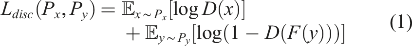
GANs training is usually challenging and suffers from mode collapse and convergence failure (Saad et al., 2024). In mode collapse, the generator is not able to learn rich feature representation and generate many duplicates, while in convergence failure, the D and G do not reach a balance, and one of them dominates the other (MathWorks, 2024). Literature review indicated that the Wasserstein loss function with gradient penalty offered more stable training compared to the traditional log-likelihood objective (Arjovsky et al., 2017; Gulrajani et al., 2017). Using the log-likelihood loss function (shown in equation (1)), the discriminator acts like a classifier that distinguishes between real and fake images. This typically leads to minimizing discontinuous functions with respect to the generators’ parameters
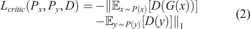
By doing so, the discriminator is transformed into a critic that scores the realness or fakeness of an image, which leads to meaningful loss curves that monitor convergence while training. The new critic loss is given by the negative of the Wasserstein-1 distance between the real and fake scores while the generator loss is now just the score the critic gave it. A stopping criterion can be established by monitoring the loss curves as a loss of zero means that G has done a great job of creating fake images that look real. The G is responsible for matching the generated image distribution with the data distribution in the target domain, and its loss is defined based on the critic average score on fake images as shown in equation (3)

Transforming the discriminator into a critic in a Wasserstein GAN is accomplished by replacing the last sigmoid layer with a linear activation. A key challenge in training traditional GANs is the issue of vanishing or exploding gradients. To address this, Arjovsky et al. (2017) proposed weight clipping as a way to enforce the 1-Lipschitz constraint, which ensures that the gradient between any two points on the function does not exceed a value of 1. However, weight clipping often led to poor performance and failed to prevent gradient issues effectively. As an alternative, Gulrajani et al. (2017) introduced the gradient penalty method, which penalizes the norm of the critic’s gradient with respect to its input, rather than constraining weights directly. Extensive experiments demonstrated that combining the Wasserstein loss with gradient penalty results in significantly more stable training.
2.2. Cycle consistency loss
A major shortcoming of traditional generative models is the lack of temporal dynamics consideration. Wind turbine data are usually composed of time series representing temperature, vibration, etc. The sequential setting of regular GANs does not adequately consider temporal correlations embedded within the time series. In this paper, we utilized CGANs architecture, shown in Figure 1, to handle time series temporal correlations. CGANs were advanced to map between a set of unlabeled and unpaired images from two domains: source x
i
∈ X and target y
i
∈ Y domains (Zhu et al., 2017). CGAN architecture.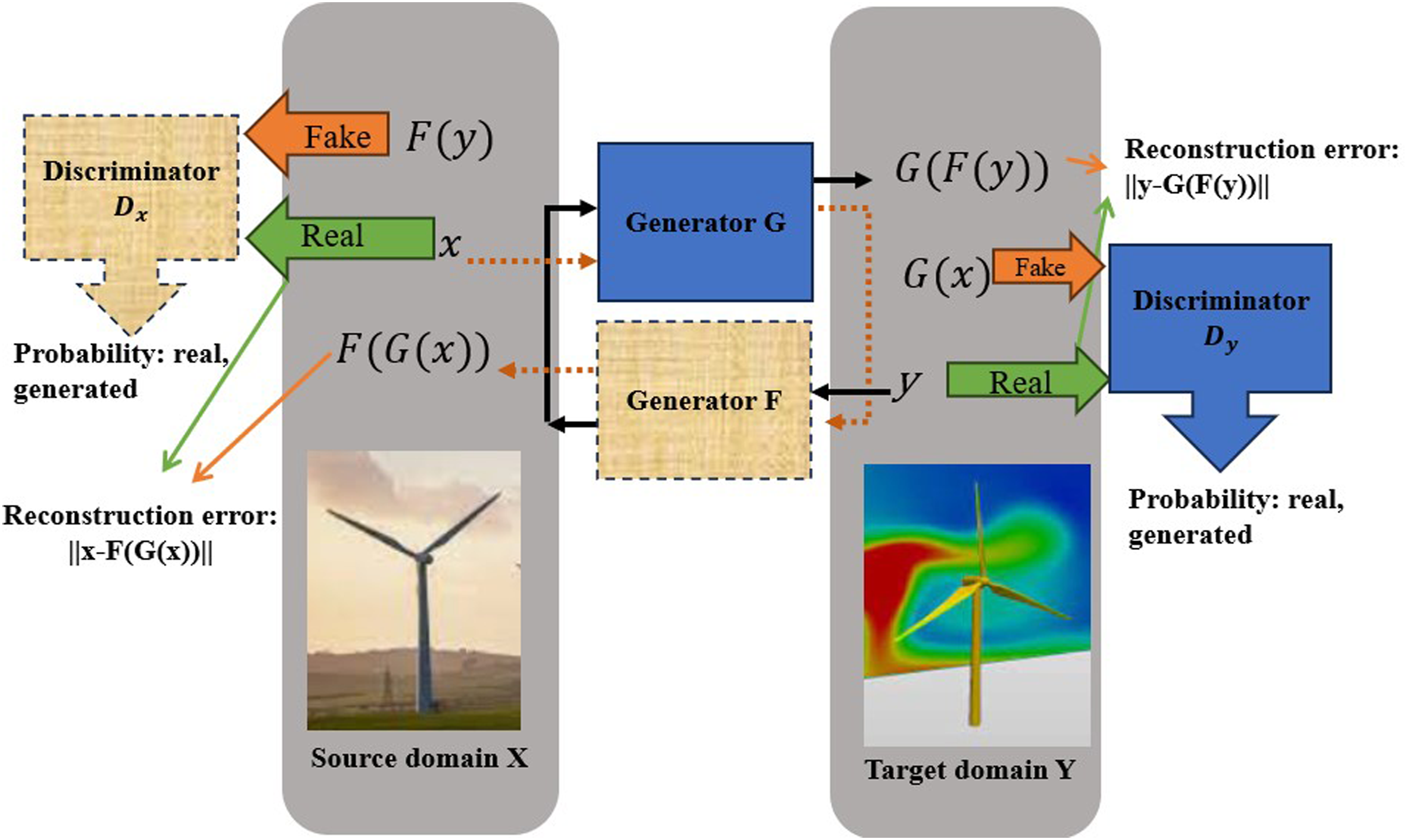
CGANs consist of two GANs: one is designated for forward mapping from X to Y, and the other GAN is designated for inverse mapping from Y to X domain. With two critics and closed-loop architecture, CGANs perform better in translating between the two spaces. The two mappings are accomplished by generators G: X → Y and F: Y → X. The two critics are responsible for distinguishing between real and generated time series: D
x
distinguishes between time series x and F(y), D
y
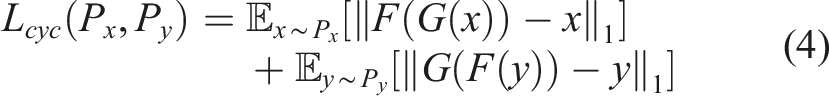
distinguishes between time series y and G(x). To prevent the learned mappings to contradict each other, cycle consistency loss is added to each generator loss function. G and F should be able to bring back each time series to its original representation, that is, forward cycle consistency x → G(x) → F (G(x)) ≈ x and backward cycle consistency y → F(y) → G (F(y)) ≈ y. As advocated in previous literature (Teng et al., 2023), L1 norm was used to define the cyclic loss as it captures the reconstruction error
2.3. Physics-informed loss function
The integration of physics principles not only enhances training performance but also ensures that the generated data adheres to the relevant physics laws, thereby preventing divergence and reducing training time. A wind turbine can be modeled as a cantilever beam with a lumped mass representing the rotor and nacelle at the top. Under this approximation, the system’s structural dynamics are governed by the following equation of motion (Hernandez-Estrada et al., 2021)
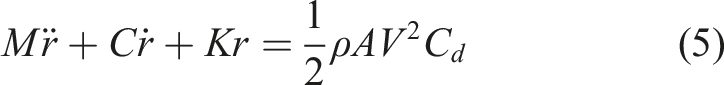
Equation (5) describes the tower-top acceleration in response to the wind loading as a second-order non-homogeneous differential equation where M represents the lumped mass of the rotor and nacelles, C is the damping coefficient, K is the structural stiffness, and
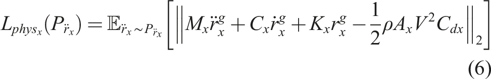
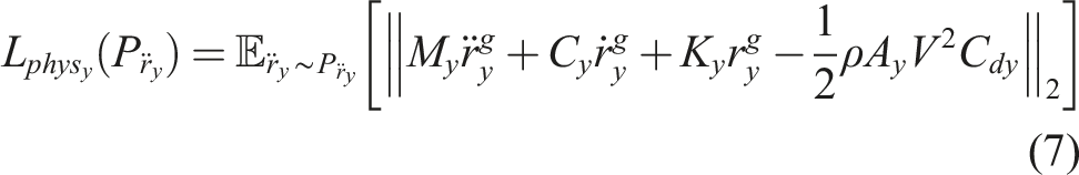
Where
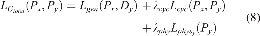
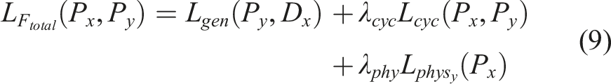
2.4. Total losses
The previously defined loss components are aggregated to form the total loss function for each of the four networks. Each network is then trained to minimize its corresponding composite loss. For the critic networks specifically, the objective is to minimize the loss toward increasingly negative values, which corresponds to maximizing the separation between the critic scores assigned to real and generated (fake) samples. The complete composite loss functions are defined as follows


3. Generators and critics network architecture
Convolutional neural network hyperparameters.
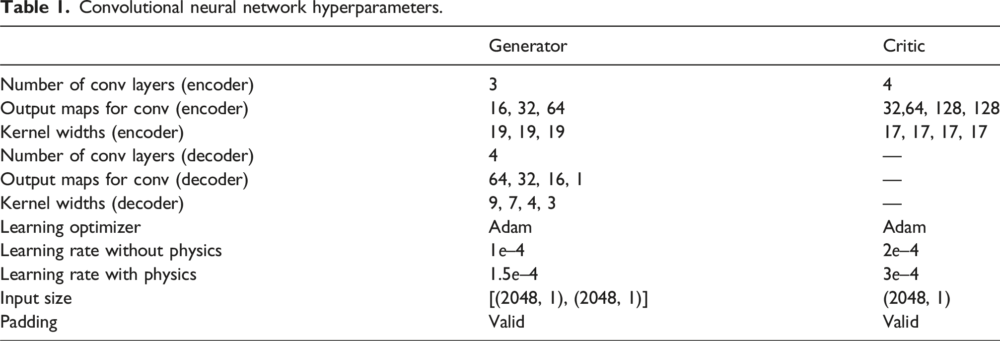
During the preprocessing phase, we initially applied same padding in our convolution operations on the time series data. In CNNs, same padding maintains the original sequence length by symmetrically adding zeros to both the beginning and end of the input. This approach is standard in image processing because images are spatially invariant, meaning the spatial relationships in images are less sensitive to boundary padding. Unlike time series, images do not rely on strict directional causality, so padding artifacts typically do not affect their internal structure or interpretation significantly. However, in the case of time series, this symmetric zero-padding introduced misalignment and artificial time delays, particularly at the sequence boundaries. These delays disrupted the model’s ability to learn precise temporal dependencies, especially at the start and end of each input window where the zero-padding created discontinuities. As a result, we observed phase shifts between the predicted and actual signals, which reduced the temporal accuracy of the model. To address the issue, we transitioned to valid padding, which avoids introducing edge artifacts by omitting any padding. While this ensures that each output element is the result of a full convolution, it comes at the cost of reducing the output length and causing a mismatch between the input and output sizes. Additionally, valid padding inherently biases the model toward the middle of the sequence, as the beginning and end values are involved in fewer convolution operations compared to those in the center. To mitigate this imbalance, we developed a custom padding scheme, illustrated in Figure 2. The dataset was preprocessed using overlapping windows, where the end of each time series segment overlaps with the beginning of the next. This is a standard technique in time series processing to promote stable training and prevent abrupt gradient shifts between consecutive batches. Our input layer crops a portion of each sequence that overlaps with adjacent windows and concatenates it to the beginning and end of the original sequence. The network then receives this extended input, which allows the first convolution layer to fully convolve, even the original boundaries. This method effectively preserves the original sequence length while ensuring that edge values are convolved multiple times, just like central values. As a result, this approach significantly reduced phase shifts and improved the alignment between predicted outputs and the original time series. Proposed custom padding scheme.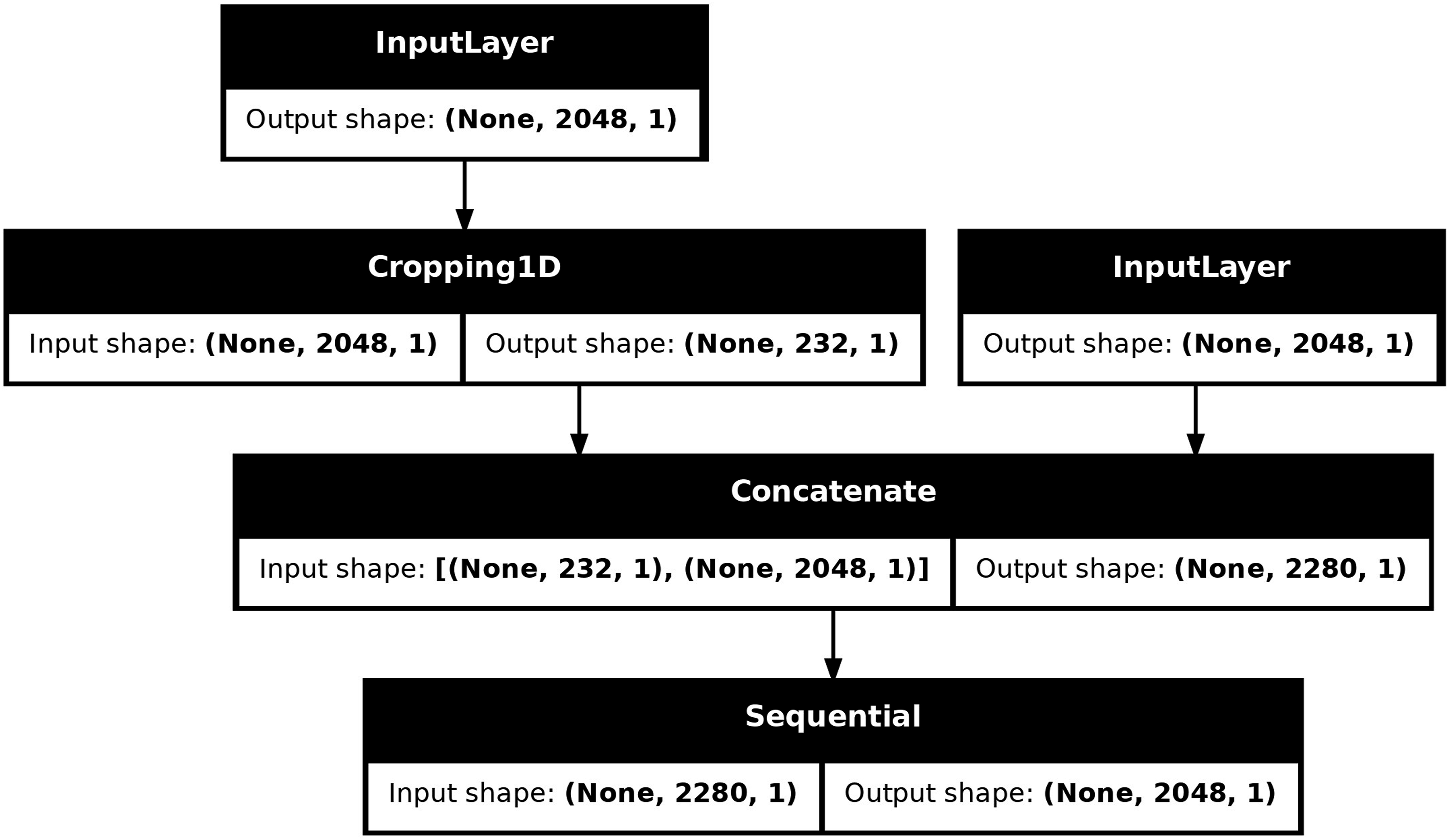
Two other key architectural parameters are the number of output feature maps and the convolutional kernel widths. In the encoder, each convolutional layer is followed by a MaxPooling layer, which reduces the spatial resolution by a factor of 2. To compensate for this down-sampling and preserve the representational capacity of the network, the number of output feature maps is doubled at each subsequent layer. In contrast, the decoder uses UpSampling layers between convolutional layers to progressively restore spatial resolution, and accordingly, the number of feature maps is halved at each stage. Relatively wide kernel sizes were used in the encoder (19 for the generator and 17 for the critic) to allow each layer to capture features across a broader receptive field. This becomes increasingly important in the deeper layers, as the receptive field of the kernel effectively doubles with each pooling operation. In the decoder, narrower kernels were employed to facilitate precise reconstruction of the signal from the learned feature maps.
This full setup was used twice, to train with and without the physics loss added to the loss function. The only difference between these setups was a slightly higher learning rate for the one with the physics loss. This was because it was observed that without the physics loss the training at the higher rate was unstable and would not converge. However, with the physics loss the network would converge and remain stable.
4. Dataset preparation and prepossessing
For the simulation data generation, stochastic inflow turbulence input was generated using the TurbSim tool (National Laboratory of the Rockies, 2024). TurbSim was developed by the National Laboratory of the Rockies to provide a numerical simulation of a full-field flow. OpenFAST receives the input from TurbSim and simulates the response of the 1.5 MW and 5 MW turbines for 3000 s. Initial training with shorter durations were found to be insufficient, as the generators tended to overfit and memorize the dataset. To mitigate this, a longer simulation was adopted to provide a more diverse and representative training set. The SDOF approximation explained above is most appropriate for steady-state operation where the first tower mode dominates. The approach may not adequately capture transient dynamics or coupled rotor-tower interactions. Therefore, the initial transient segment (first 40 s) was excluded, and the training dataset was restricted to the steady-state regime. While this simplification enables stable and efficient training for the present single channel tower-top acceleration signal, extension to multichannel measurements or coupled subsystem dynamics would require higher order or coupled physics formulations. All datasets were standardized using zero-mean, unit-variance normalization. The time series data were then segmented into overlapping windows to increase the effective dataset size while preserving temporal correlations. The degree of overlap was dependent on the generator architecture; in the final configuration, each 2048-point sample overlapped by 1816 data points with its neighboring sample. From the generated data, the first 1600 samples were allocated for training. This number was chosen to align with a batch size of 32, allowing efficient use of computational resources during each training step. An additional 850 samples were reserved for testing, with a 100-sample gap separating the training and testing sets to avoid data leakage. This dataset partitioning is illustrated by the wind input in Figure 3. Simulated wind speed input with labeled data section.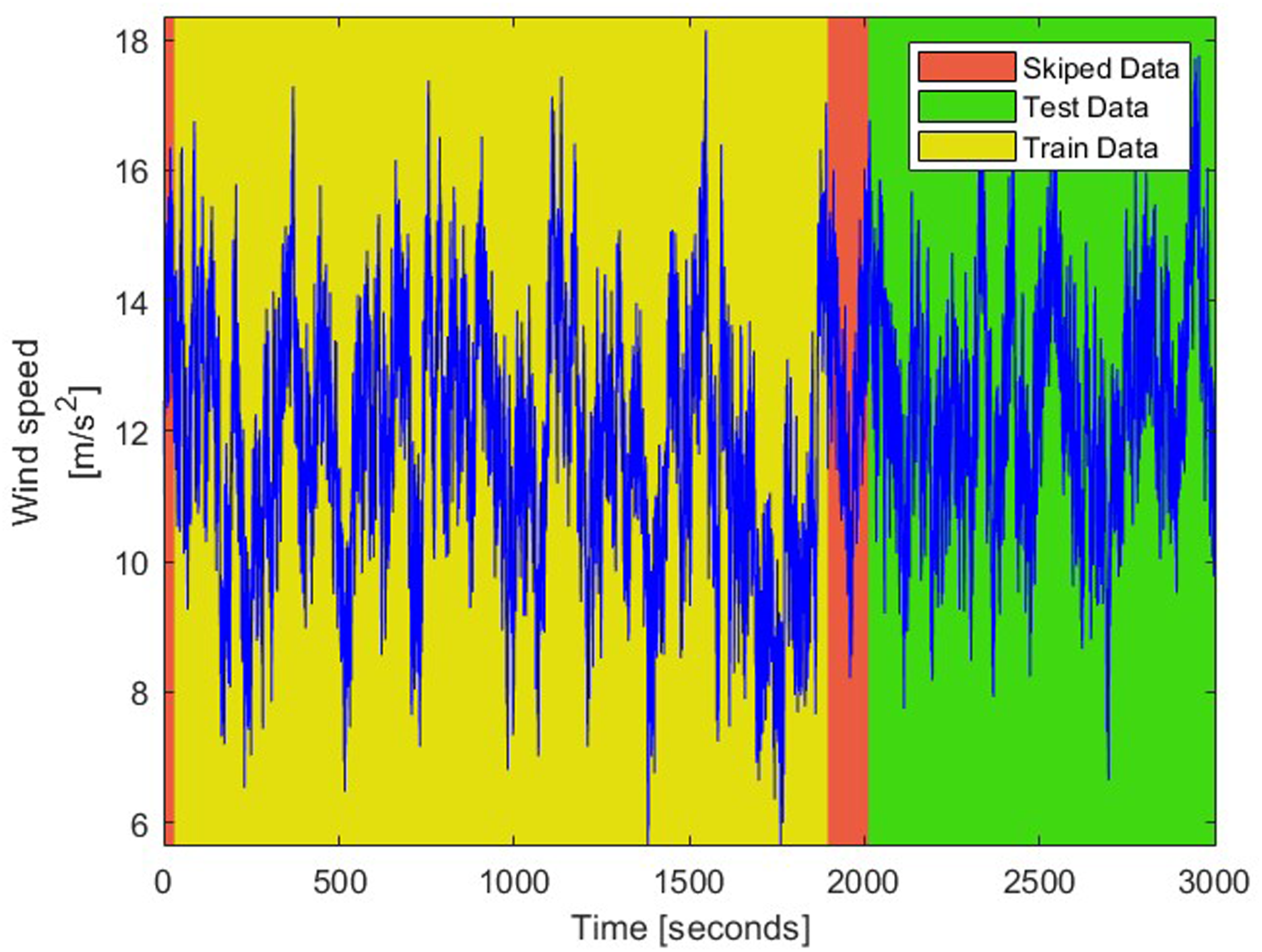
5. Results and discussion
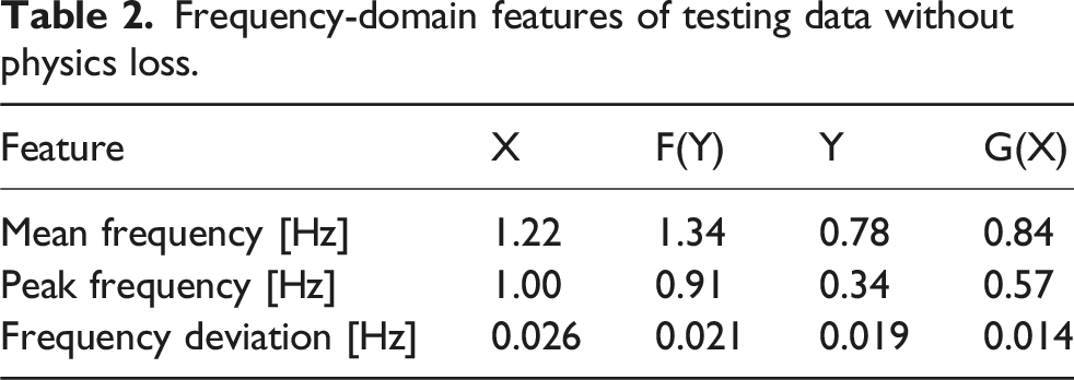
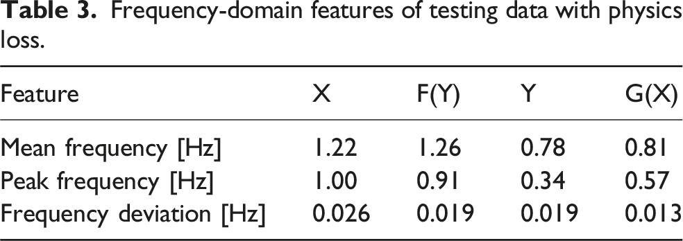
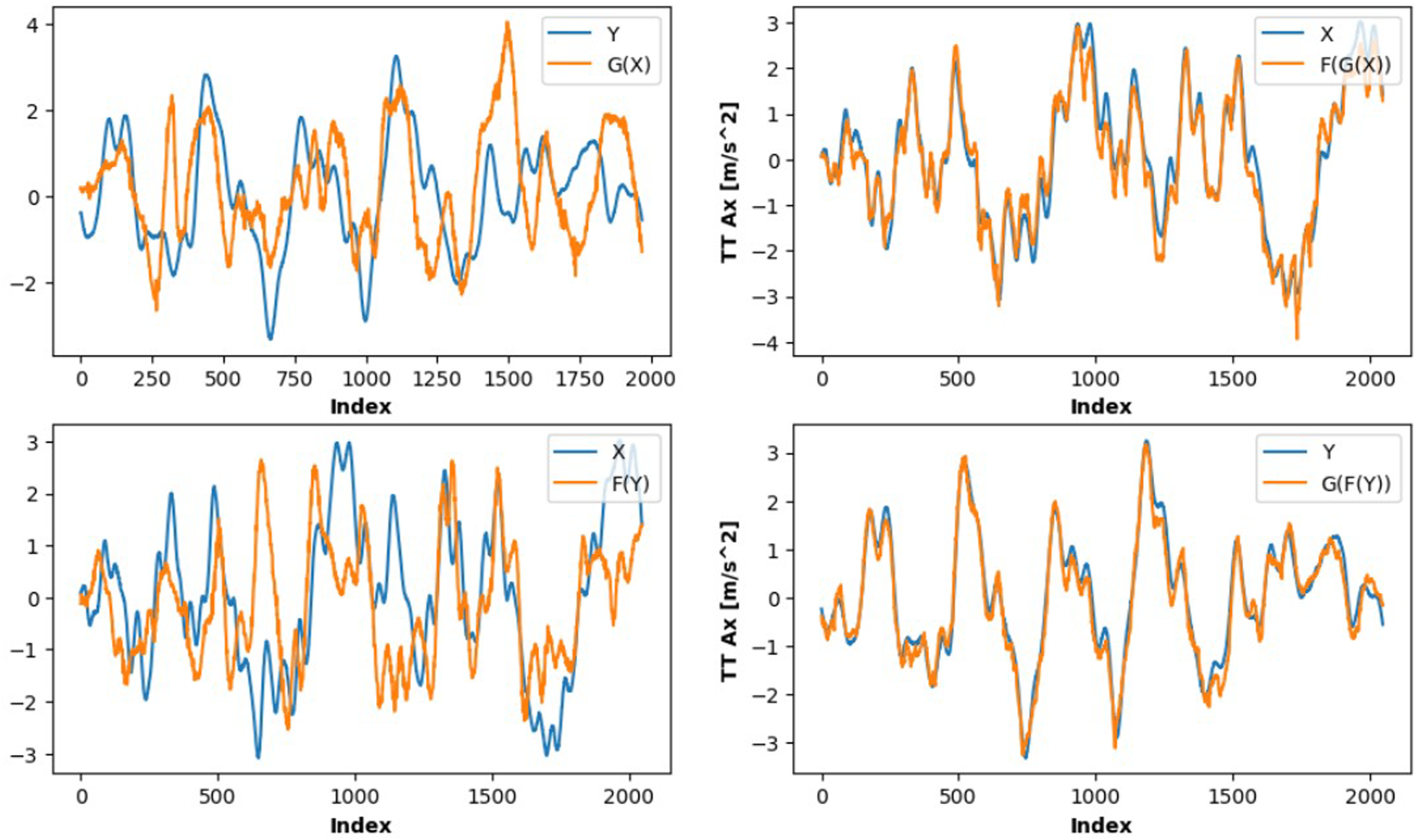
The CGAN, with and without the physics-informed loss function, was trained until convergence of the generator and critic losses, which served as the stopping criterion. Convergence was defined as the point at which the average difference between the critic score for real and generated samples fell below a threshold of 10. The baseline model, trained without the physics-informed loss, required approximately 73,000 epochs to reach convergence. In contrast, the physics-informed model converged significantly faster, requiring only 13,000 epochs to achieve the same criterion, representing an 82% reduction in training time. The physical quantity examined throughout this section is the tower-top acceleration which is measured at the nacelle level for both the 1.5 MW and 5 MW turbines. To evaluate G and F performance in mapping between different domains, we first examine the power spectral density (PSD) of the generated signals, as shown in Figure 4. The PSDs of the original signals compared with the generated counterparts exhibit a very similar spectral distribution. In both cases, without and with physics incorporation, the dominant energy is concentrated at low frequencies (<1.5 Hz), with smaller harmonics appearing at higher frequencies. The quantitative metrics in Tables 2 and 3 further support this observation. For X and its generated counterpart F(Y), the mean and peak frequencies remain close (1.22 vs 1.34/1.26 Hz and 1.00 vs 0.91 Hz, respectively), and the frequency deviation is slightly lower for F(Y) (0.026 vs 0.021/0.019 Hz). Similarly, for Y and G(X), both the mean and peak frequencies are well preserved (0.78 vs 0.84/0.81 Hz and 0.34 vs 0.57 Hz), with G(X) again exhibiting a reduced frequency deviation. The tower-top acceleration PSD of the reference and generated signals. Frequency-domain features of testing data without physics loss. Frequency-domain features of testing data with physics loss.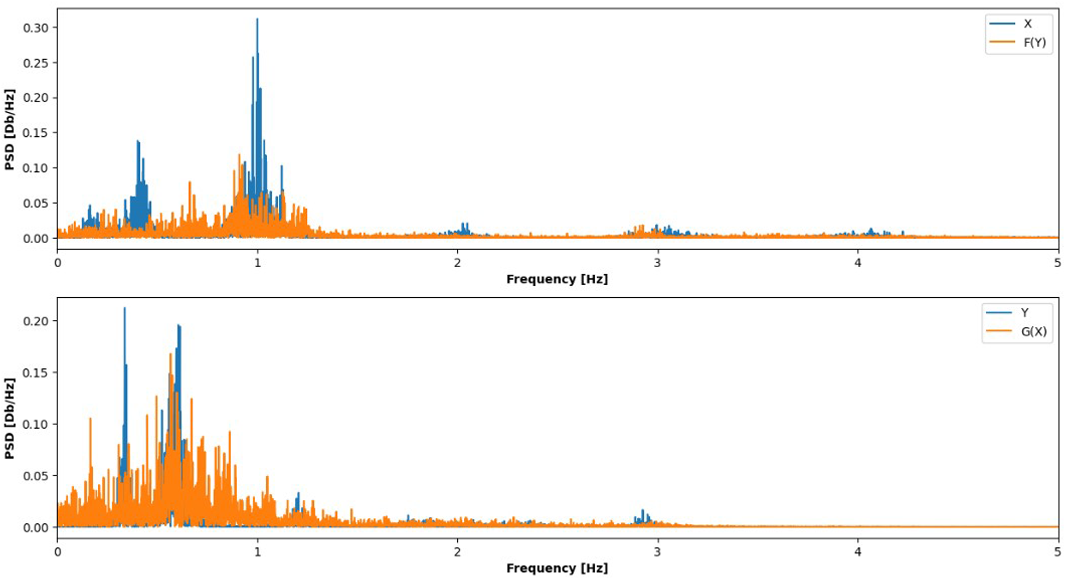
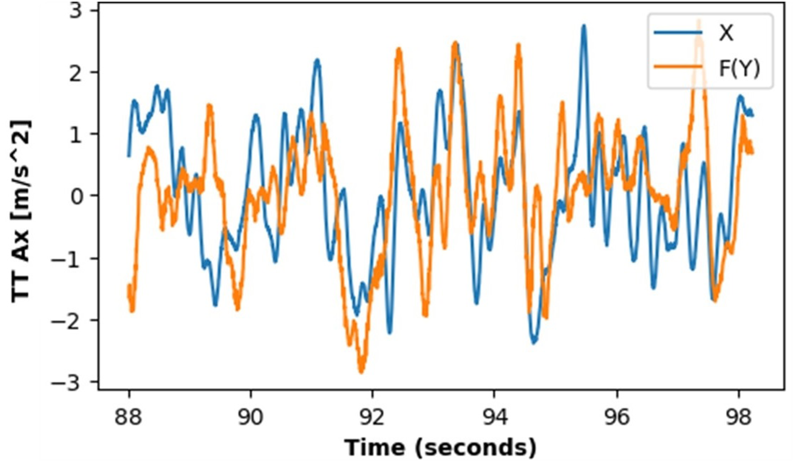
Figures 5 and 6 show time-domain comparisons between the original signals and their generated counterparts, as well as the cycle consistency reconstructions. The generated signals (orange curves) closely follow the dynamics of the original signals (blue curves), capturing both the amplitude and phase variations over time. Although slight amplitude mismatches are visible, the overall temporal structure is preserved and the incorporation of the physics-informed loss improved the coefficient of determination R2 by approximately 30%, while reducing the RMSE from 1.39 to 1.1 m/s2. For the cycled signals, the results show near-perfect mapping, indicating that the bidirectional mappings not only approximate the transformations between domains but also maintain consistency when cycled back to the original domain. This highlights the CGAN ability to preserve essential signal dynamics in both forward and inverse mappings. To further assess robustness and practical relevance, we conducted a preliminary sensitivity analysis by increasing the turbulence intensity from IEC Category B to Category A. At a reference wind speed of 12 m/s, this corresponds to an increase of approximately 3% in turbulence intensity. The trained physics-informed model was evaluated using the new simulation data without retraining. The prediction performance remained stable as shown in Figure 7, with the RMSE remaining approximately 1.1 m/s2, indicating that the learned domain mapping is not highly sensitive to moderate changes in inflow turbulence characteristics. Baseline model 10 s prediction (from 2662 s to 2672 s). Physics-informed model 10 s prediction (from 2662 s to 2672 s). Physics-informed model prediction under increased turbulence intensity (IEC Category A).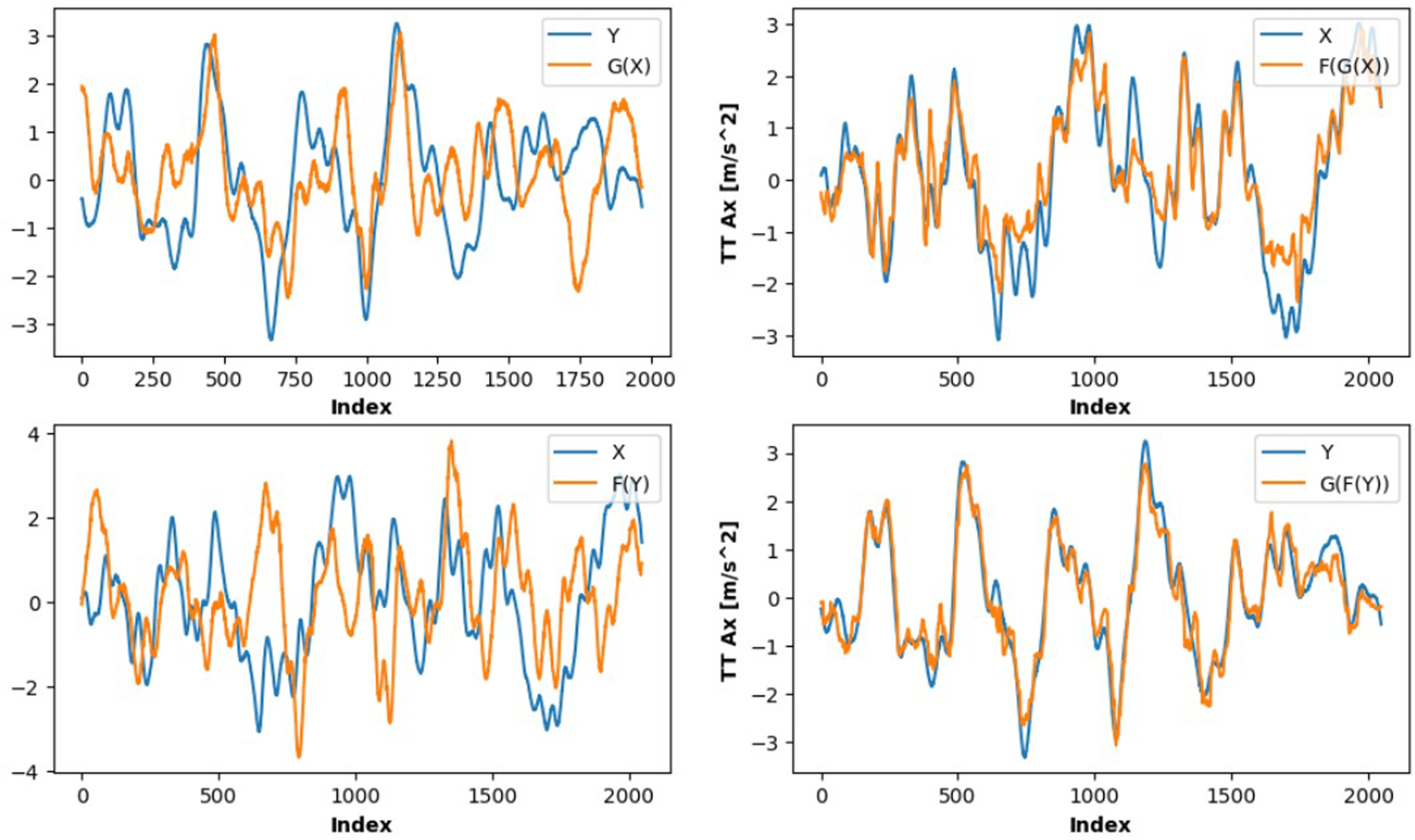
6. Conclusions
In this paper, a physics-informed CGAN was proposed to bridge the probability distribution gap between simulated 1.5 MW and 5 MW wind turbines. The generated signals preserved essential temporal dynamics, dominant spectral peaks, and low-frequency energy content in both time and frequency domains. Incorporating a physics-informed loss function improved the R2 values by 30%, reduced the RMSE from 1.39 to approximately 1.1 m/s2, and decreased training time by 82%. Furthermore, under increased wind turbulence intensity, the RMSE remained stable at approximately 1.1 m/s2. The proposed methodology enables domain translation between simulated turbines of different ratings and is architecturally extensible to multichannel sensor data. Validation against real operational turbine data and extension to other subsystems remain important directions for future work.
Footnotes
Acknowledgments
This work was supported in part by the U.S. Department of Energy, Office of Science, Office of Workforce Development for Teachers and Scientists (WDTS) under the Visiting Faculty Program (VFP). This work was authored in part by the National Laboratory of the Rockies for the U.S. Department of Energy (DOE), operated under Contract No. DE-AC36-08GO28308. Funding provided by U.S. Department of Energy Critical Minerals and Energy Innovation Integrated Energy Systems Office. The views expressed in the article do not necessarily represent the views of the DOE or the U.S. Government. The U.S. Government retains and the publisher, by accepting the article for publication, acknowledges that the U.S. Government retains a nonexclusive, paid-up, irrevocable, worldwide license to publish or reproduce the published form of this work, or allow others to do so, for U.S. Government purposes.
Funding
The authors disclosed receipt of the following financial support for the research, authorship, and/or publication of this article: This work also supported in part by the National Science Foundation Research Experiences for Undergraduates program (grant number 2244119) through Dr. Faisal Aqlan’s lab at the University of Louisville.
Declaration of conflicting interests
The authors declared no potential conflicts of interest with respect to the research, authorship, and/or publication of this article.