Linear time complexity analysis of time-periodic delayed systems with multiplication free semi-discretization method

Abstract

This study introduces the multiplication free semi-discretization method (MFSD), a novel approach for the efficient stability and fixed-point analysis of time-periodic delayed differential equations (DDEs). Efficient stability prediction is critical for mitigating instabilities in mechanical systems, such as machine tool chatter in milling and vibration in delayed control systems, where high-accuracy modelling often leads to prohibitive computational costs. Unlike traditional semi-discretization methods that are burdened by high computational demands due to repeated matrix multiplication, the MFSD method leverages a composite mapping structure inspired by collocation techniques to achieve linear time complexity $(O (p^{1}))$ .The performance of the method is validated through extensive spectral analysis of the delayed Mathieu equation and further demonstrated on three practical engineering cases: a seasonal biological model, a multi-cutter turning system with spindle speed variation, and a finite-element-method-based longitudinal vibration of an elastic beam under delayed boundary feedback. Results demonstrate that MFSD maintains linear scaling even for system resolutions up to 10⁶, enabling high-fidelity stability mapping even for high-dimensional structural dynamics that were previously computationally inaccessible. The algorithm is provided as an open-source tool via the SemiDiscretizationMethod.jl package to support the vibration and control research community.

Keywords

time-delay semi-discretization time complexity stability periodic solution

1. Introduction

Delayed differential equations (DDEs) play a pivotal role in modelling dynamics where time delays are intrinsic, such as in control systems (Åström and Murray, 2021; Habib et al., 2016; Bartfai and Dombovari, 2022), biological processes (Stepan, 2009; Insperger et al., 2022; Kovacs and Insperger, 2018), vehicle dynamics (Li et al., 2024; Mi et al., 2024) and mechanical vibrations (Bartfai et al., 2024; Horvath and Takacs, 2023; Sanz-Calle et al., 2024; Zhang and Xi, 2022). The stability analysis of DDEs is crucial for predicting system behaviour and ensuring reliability (Ali et al., 1998; Kiss et al., 2022; Borgioli et al., 2020). However, calculating the stability of DDEs poses significant computational challenges, especially when it is critical to capture the system’s dynamics accurately (Zatarain and Dombovari, 2014; Toth et al., 2017; Lehotzky et al., 2016; Lichtner et al., 2011; Itovich et al., 2024).

There are several available methods, most of them in frequency- and time domains. In the frequency domain, conventional approaches, such as calculating stability boundaries, involve the critical frequency as an additional parameter (Stepan, 2009; Ozturk and Budak, 2008; Bachrathy and Stepan, 2013). These methods often require complex integration along the frequency parameter, limiting their practicality. Alternatively, time-domain methods, including collocation-based and integration-based strategies, offer solutions but with their own sets of challenges. Collocation methods and time-finite element methods (Butcher and Bobrenkov, 2011; Lehotzky and Insperger, 2016; Lehotzky et al., 2018; Vyasarayani et al., 2014; Breda et al., 2005; Bayly et al., 2003), known for their excellent convergence properties, face difficulties with discontinuities, making them less robust and more complex to implement for general cases.

Despite these limitations, collocation-based approaches continue to be applied successfully in structural dynamics problems involving delay, particularly when combined with finite element discretization in space. For example, recent studies have applied Chebyshev-based discretization to analyse the delayed stability of delaminated composite beams subjected to follower forces (Szekrényes, 2023, 2025), demonstrating the practical relevance of such methods in vibration problems with distributed parameters and time-delay feedback.

Our focus is on an integration-based strategy, specifically the semi-discretization method (Insperger and Stépán, 2002; Insperger and Stepan, 2004; Insperger and Stépán, 2011; Sykora and Bachrathy, 2020) and its alternatives (Ozoegwu, 2018; Insperger, 2010; Liu et al., 2024; Yang et al., 2023), such as full-discretisations. Despite their limited convergence, these methods are favoured for their ease of implementation. The trade-off between convergence limitations and implementation ease is often acceptable, especially when handling systems with non-smooth behaviour.

Traditionally, these methods involve repeated matrix multiplication, significantly increasing CPU time demands. In Henninger and Eberhard (2008), the method has been optimised based on the special matrix structure leading to quadratic time complexity. Current literature primarily concentrates on improving the eigenvalue convergence rate rather than computational efficiency, attempting to achieve more accurate eigenvalues at lower resolution (Ozoegwu, 2018).

However, it’s crucial to note the trend in newer techniques that promise better time complexity of the eigenvalues of the mapping with fewer resolution steps. Often, these methods are demonstrated with a very limited resolution range (<100) (Ozoegwu, 2018; Liu et al., 2024; Yang et al., 2023), and usually not in a log–log scale, making it challenging to discern true convergence rates and the time complexity. At lower resolution levels, the nuances in implementation can significantly influence outcomes, potentially resulting in inaccurate conclusions. Furthermore, these higher-order methods have similar difficulties with discontinuities as the collocation methods.

We have to note that there is a new class of time-domain methods, which are based on direct simulation of the investigated DDE (Zatarain and Dombovari, 2014; Zatarain et al., 2015; Toth et al., 2017). These methods iteratively extract the eigenvalue/eigenvectors of the underlying mappings from the simulated timeseries and promise excellent work-precision diagrams. Unfortunately, their iterative nature makes it hard to compare them based on time complexity to the above-mentioned time domain methods where exact resolution-CPU time can be determined.

This study extends the integration-based time-domain methods by introducing a novel approach inspired by collocation techniques, enabling a linear time complexity implementation. The main aim is to overcome the computational limitations of traditional semi-discretization methods by eliminating the need for repeated matrix multiplications. The development is specifically presented for the semi-discretization method but is applicable to any approach that involves step-wise matrix multiplication, significantly reducing the computational cost.

Section 2 outlines the fundamental steps of the semi-discretization method and analyses its computational time complexity. Additionally, it briefly reviews prior advancements aimed at improving its efficiency. In Section 3, we introduce the multiplication free semi-discretization (MFSD) method, detailing the formulation of left and right mapping matrices for various time-period and time-delay ratios. Section 4 evaluates the computational performance of the proposed approach through high-resolution work-precision diagrams for both the conventional semi-discretization (SD) method and the introduced MFSD. The results clearly demonstrate that the new method achieves linear time complexity.

We’ve implemented our method in the publicly available SemiDiscretizationMethod.jl package, aiming to contribute to the broader community’s ability to analyse and predict the behaviour of systems governed by DDEs more efficiently.

2. Main contributions

While the algebraic concept of direct matrix composition has been previously mentioned for specific cases (e.g. in Hamann and Eberhard (2018) for T = τ), its profound algorithmic implications have remained unrecognised. This study establishes MFSD as a comprehensive computational framework with the following core contributions:

• Discovery of Linear Complexity: We demonstrate that MFSD, when coupled with sparse matrix data structures, reduces the time complexity of stability analysis from nearly cubic $O (p^{2.8})$ to strictly linear $O (p^{1})$ .

• Generalisation to Arbitrary Ratios: We develop the mathematical framework necessary to handle arbitrary period-to-delay ratios (T ≠ τ), providing a unified solution for general time-periodic systems.

• Algorithmic Equivalence: We demonstrate that the method is an exact algebraic rearrangement of the traditional semi-discretization mapping, ensuring identical numerical results without loss of accuracy.

• Open-Source Tool: We provide a highly optimised implementation in the publicly available SemiDiscretizationMethod.jl package, capable of evaluating previously impossible discretization resolutions (e.g. p = 10⁶).

3. Basics of the semi-discretization method

Consider the linear delayed dynamical system (Insperger and Stépán, 2011) of the form

\dot{x} (t) = A (t) x (t) + B (t) x (t - τ),

(1)

where

x (t) \in R^{d}

is the time dependent state vector of the d dimensional first order system. The system matrices A(t) and

B (t) \in R^{d \times d}

are the T-periodic time-varying coefficient matrices, and τ is the time delay. The initial state of delay systems is described via a function

x (t) = ø (t) [- τ, 0] \mapsto R^{d}

. As the derivative

\dot{x} (t)

requires not only the current state x(t) but the delay state x (t − τ) as well, therefore the notation x^(t) (ϑ), ϑ ∈ [t − τ, t] will be used to denote a solution segment that includes the entire state history between times t − τ and t.

Finding the stability of the system (1) requires the spectral properties of the mapping that maps x^(t) (ϑ) a full period T forward to x^(t+T) (ϑ). In the semi-discretization method, the continuous state-space is sampled over a uniform time-grid with resolution Δt, resulting in the sampled states x_i = x (t_i) at times t_i = iΔt. Figure 1 shows the sketch of corresponding discretised one-step- and one-period mappings.

Figure 1.

Schematic representation of the semi-discretization method. The vector 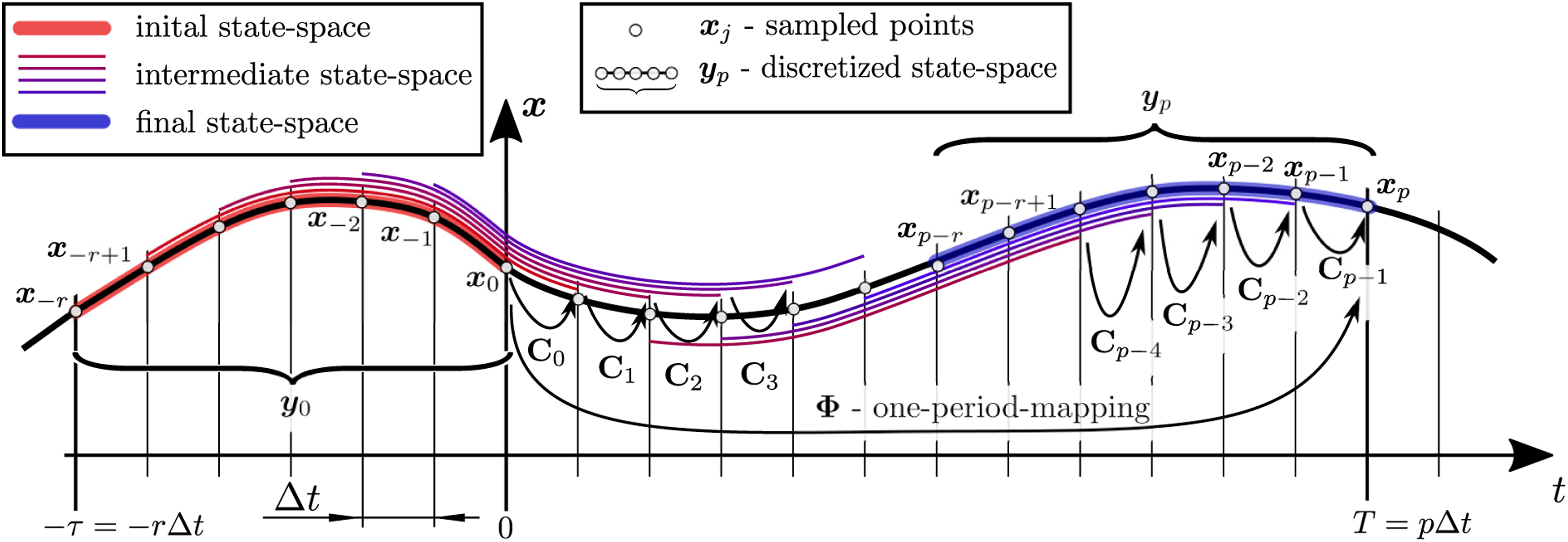y₀ of the sampled x_i (i ∈ [−r, 0]) states are mapped one time step ahead by the one-step matrices C_j (j ∈ [0, p − 1]) sequentially. The one-period mapping can be performed directly by the monodromy matrix Φ based on equation (7).

Using the discretised values x_i, the solution segment $x^{(t_{i})} (θ)$ is represented by the vector

y_{i} = {[\begin{matrix} x_{i} & x_{i - 1} & x_{i - 2} & \dots & x_{i - r} \end{matrix}]}^{⊤},

(2)

where

r \geq τ / Δ t .

(3)

The usual selection for the number of the sampled points is $r = ⌈ τ / Δ t ⌉ \in Z_{+}$ .

In order to capture the T-periodic mapping, the time increment Δt is required to be an integer fraction $p \in Z_{+}$ of period T, that is, T = pΔt, therefore, in practice p is selected first, leading to Δt = T/p. In the following description, for the sake of simplicity, the time delay τ is assumed to be τ = rΔt.

The main idea of the semi-discretization method is that the time-varying components: A(t), B(t) and x (t − τ) are considered to be constant for each Δt time segment. With this approximation, an analytical formula can be provided for the next sampled state x_i+1 using the elements of y_i see equation (2):

x_{i + 1} = P_{i} x_{i} + R_{i} x_{i - r} .

(4)

In case Δt is chosen in a manner that τ = rΔt and T = pΔt, and A⁻¹ (t_i) exists, then for zeroth-order semi-discretization (Insperger and Stépán, 2002) the coefficient matrices P_i and R_i have closed form solutions, that is,

P_{i} = e^{A (t_{i}) Δ t}

and

R_{i} = (e^{A (t_{i})} - I) A^{- 1} (t_{i}) B (t_{i})

. For the definition of P_i and

R_{i} \in R^{d \times d}

in higher-order cases¹, see Insperger et al. (2008). To cover a full period, the mapping (4) should be repeated for p times. Without loss of generality, we set t = 0 as the starting point; in this case, we need to repeat the mapping (4) for i = 0, 1, …, p − 1.

Using equation (4), the one-step mapping from y_i to y_i+1 is defined by the one-step matrix $C_{i} \in R^{(r + 1) d \times (r + 1) d}$ as:

C_{i} = [\begin{matrix} P_{i} & 0 & 0 & \dots & 0 & R_{i} \\ I_{d} & 0 & 0 & \dots & 0 & 0 \\ 0 & I_{d} & 0 & \dots & 0 & 0 \\ 0 & 0 & I_{d} & \dots & 0 & 0 \\ ⋮ & ⋱ & ⋮ \\ 0 & 0 & 0 & \dots & I_{d} & 0 \end{matrix}],

(5)

leading to the state-space representation:

y_{i + 1} = C_{i} y_{i},

(6)

where

I_{d} \in R^{d \times d}

are identity matrices. The subdiagonal blocks in C_i represent the temporal shift of the sampled state history between y_i and y_i+1.

Starting from the initial discretized state y₀, p recursive applications of the one-step mapping in equation (6) yield the state-space after one period:

y_{p} = C_{p - 1} \dots C_{1} C_{0} y_{0} .

(7)

The transition over a full period T is governed by the Monodromy matrix (or Floquet transition matrix) $Φ \in R^{(r + 1) d \times (r + 1) d}$ , defined as:

Φ ≔ C_{p - 1} \dots C_{1} C_{0},

(8)

such that the one-period mapping is represented by y_p = Φy₀.”

The stability properties of the trivial solution can be determined based on the spectral radius of the monodromy matrix (or Floquet transition matrix) Φ. The fixed point is asymptotically stable if the spectral radius Φ is smaller than 1, that is, the absolute value of the largest eigenvalue of Φ is smaller than 1 (|μ_max| < 1).

3.1. Time complexity of the semi-discretization method

The time complexity of the traditional semi-discretization method was thoroughly analysed in Henninger and Eberhard (2008). Here we will focus on the effect of the time-step Δt on the spectral radius (|μ_max|) only. Note that both p and r are inversely proportional to Δt. The semi-discretization algorithm has the following key steps:

• The computation of P_i and R_i requires the calculation of matrix exponents, which can take a significant portion of the time spent on computation for high-dimensional systems (d >> 1). This step needs to be performed p times, once for each time step, therefore, it has linear time complexity $O (Δ t^{- 1})$ .

• The one-step matrices C_i have (r + 1)²d² elements. However, there are simple optimisation, that reduce the memory required. For example, the array containing C₀ can be reused for C₁, C₂, …. Hence, after its use, it is no longer needed. Using sparse matrices further reduce memory requirements, as there are (r + 2)d² elements that change for each C_i. Combining sparse matrices with so-called ‘lazy arrays’, where some elements of the matrix are computed upon indexing the array can further reduce memory requirements. With this technique, there is no need to store the identity matrices I, as the location of the non-zero elements are distributed along an off-diagonal (easy-to-capture pattern). Therefore, the complexity of this step has linear complexity $O (Δ t^{- 1})$ when implemented properly.

• The generation of monodromy matrix Φ can be the most time-consuming step, hence it requires p multiplications of $R^{(r + 1) d \times (r + 1) d}$ sized matrices. The schoolbook multiplication has cubic complexity leading to $O (p {((r + 1) d)}^{3})$ , however, high-end algorithms can reach $\sim 2.37$ complexity (Le Gall, 2014). In the practical range of p values, mostly the Strassen-algorithm (Strassen, 1969) is used (e.g. in Matlab, BLAS implementation), which has $\sim 2.8$ complexity. In our case, it leads to approximately $O (p {((r + 1) d)}^{2.8}) = O (Δ t^{- 3.8})$ .

• The final step is to compute the eigenvalue with the largest magnitude of $Φ \in R^{(r + 1) d \times (r + 1) d}$ . In case of full matrix representation of Φ this can be solved with $O ({(r + 1)}^{3} d^{3}) = O (Δ t^{- 3})$ (through SVD factorisation), or $O (s (r + 1) d^{2}) = O (Δ t^{- 1})$ for sparse matrices, where s is the average number of non-zeros in Φ (through a row based on Lanczos algorithm (Saad, 2011)). Note, Φ is typically similar to a full upper triangular matrix, thus s ∼ p leading to quadratic time complexity $O (Δ t^{- 2})$ .

The most critical part is the recursive matrix multiplication in equation (7), therefore, in the literature, many different methods were proposed to speed up this step. In the following section, we will present the most common ones.

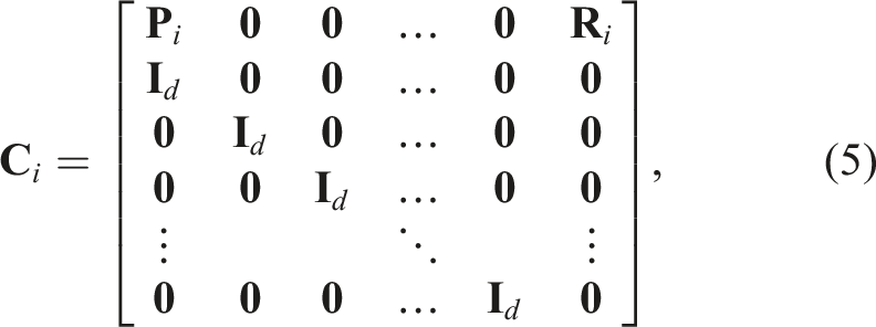
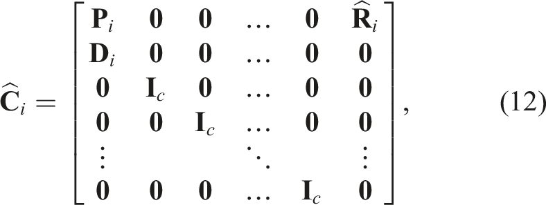
Following the history of the necessary state components only in many problems, not all the component of the delayed state x (t − τ) is used in the governing equation, that is, the rank of B(t) is not full. This is more evident in the following form, which is commonly used in control theory:

\begin{align} \dot{x} (t) & = A (t) x (t) + \hat{B} (t) u (t - τ) \end{align}

(9)

\begin{align} u (t) & = D (t) x (t), \end{align}

(10)

where $u (t) \in R^{c}$ is the control input, D is $R^{c \times d}$ and $\hat{B}$ is $R^{d \times c}$ . These coefficients generate $B (t) = D (t) \hat{B} (t)$ for equation (1). Based on equation (9) and (10), we can reduce the size of y_i by storing only the relevant components, yielding

{\hat{y}}_{i} = {[\begin{matrix} x_{i} & u_{i - 1} & u_{i - 2} & \dots & u_{i - r} \end{matrix}]}^{⊤},

(11)

where

{\hat{y}}_{i} \in R^{d + c r}

. In this case, the one-step mapping

{\hat{y}}_{i + 1} = {\hat{C}}_{i} {\hat{y}}_{i}

is formulated based:

{\hat{C}}_{i} = [\begin{matrix} P_{i} & 0 & 0 & \dots & 0 & {\hat{R}}_{i} \\ D_{i} & 0 & 0 & \dots & 0 & 0 \\ 0 & I_{c} & 0 & \dots & 0 & 0 \\ 0 & 0 & I_{c} & \dots & 0 & 0 \\ ⋮ & ⋱ & ⋮ \\ 0 & 0 & 0 & \dots & I_{c} & 0 \end{matrix}],

(12)

where I_c is the indentitiy matrix with size

R^{c \times c}

. The size reduction can be significant if c ≪ d, leading to the size of the mondorodmy matrix

R^{(d + c r) \times (d + c r)}

. However, this will not improve the complexity of the calculation as a function of the time-step (it remains

O (p {(d + c r)}^{2.8}) = O (Δ t^{- 3.8})

), but it does provide a constant improvement of approximately (c/d)^2.8.

Exploitation of the matrix structure: In Henninger and Eberhard (2008), the recursive matrix multiplication of C_i (or ${\hat{C}}_{i}$ ) matrices is greatly reduced by exploiting the special structure of the matrix. In this method, the step matrix is considered to comprise three main blocks: ${[P_{i} D_{i}]}^{⊤}$ , $[{\hat{R}}_{i}]$ and a diagonal block [I_(r−1)c]. The multiplication is performed by the first two blocks with the corresponding row of the preceding step matrix. The multiplication with the unit-block matrix provides a shift in the final result, so it is not performed numerically. Note that with proper memory management, even the movement of the data (the shift) can be eliminated, hence, the final position of the elements in $\hat{Φ}$ can be determined a priori. With this formulation, the time complexity is reduced to $O (Δ t^{- 2})$ (Henninger and Eberhard, 2008).

Sparse matrix representation: It is observed that most of the elements of the matrix C_i are zero, suggesting that a sparse matrix data structure can substantially enhance computational speed. Following a detailed numerical analysis (discussed later), it has been determined that the complexity associated with constructing Φ can be approximated as $O (Δ t^{- 2.5}) \dots O (Δ t^{- 2.8})$ . This strategic optimisation, which is a straightforward one-line implementation, achieves a comparable level of efficiency improvement to that outlined in the preceding subsection; however, the sparse matrix manipulation has a slight overhead.

Note that this sparse representation is not so efficient at the last few steps of the multiplication, where the resulting matrix typically becomes an almost full triangular matrix.

The improvements discussed above represent the most commonly adopted strategies to enhance the computational efficiency of the semi-discretization method. However, the authors are unaware of any other numerically validated optimisation that achieves a linear computational complexity.

4. Multiplication free one-period Mapping

In the following sections, the ‘Multiplication Free Semi-Discretization’ (MFSD) is introduced and analysed for different T/τ ratios. The linear time complexity is presented through a detailed numerical test, and it is compared to the Semi-Discretization method, both combined with a sparse matrix representation of the corresponding mapping matrices.

In the Semi-Discretization method, each multiplication with the one-step matrices C_i approximates an integration step of length Δt of the state variable y_i, while the multiplication with the Φ matrix approximates a one-period integration of length T. In the proposed method, our viewpoint is different: it is sufficient to represent the dynamics by means of equation (4) for each time step to find the spectral properties, similarly to the collocation methods (Butcher and Bobrenkov, 2011; Lehotzky and Insperger, 2016; Bayly et al., 2003).

This type of direct composition was briefly presented for SD in Hamann and Eberhard (2018) for T = τ only. However, it was viewed primarily as an alternative algebraic representation with a disadvantageously larger state vector. 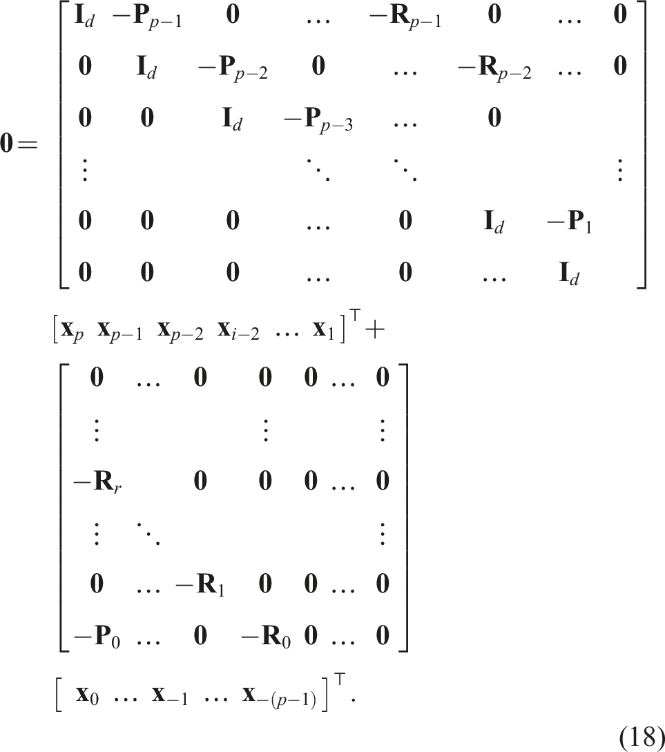Its banded structure and very sparse properties, its generalisation to arbitrary period-to-delay ratios, and its profound effect on reducing the computational time complexity to $O (p^{1})$ were completely unrecognised and unanalysed—aspects which form the primary focus of the following sections.

The first step is to rewrite the one-step mapping (4) to the form:

0 = I_{d} x_{i + 1} - P_{i} x_{i} - R_{i} x_{i - r},

(13)

leading to the matrix form:

\begin{aligned} 0 = & [\begin{matrix} I_{d} & - P_{i} & 0 & 0 & \dots & 0 & - R_{i} \end{matrix}] \\ \times {[\begin{matrix} x_{i + 1} & x_{i} & x_{i - 1} & x_{i - 2} & \dots & x_{i - r} \end{matrix}]}^{⊤}, \end{aligned}

(14)

as shown in the visual representation in the top section of Figure 2.

Figure 2.

(top) Schematic representation of one-step equation of the semi-discretization method; (bottom) representation of all the equations of each time step (red and blue rectangle represent the collections of states which belong to the initial and final sampled state-space, respectively).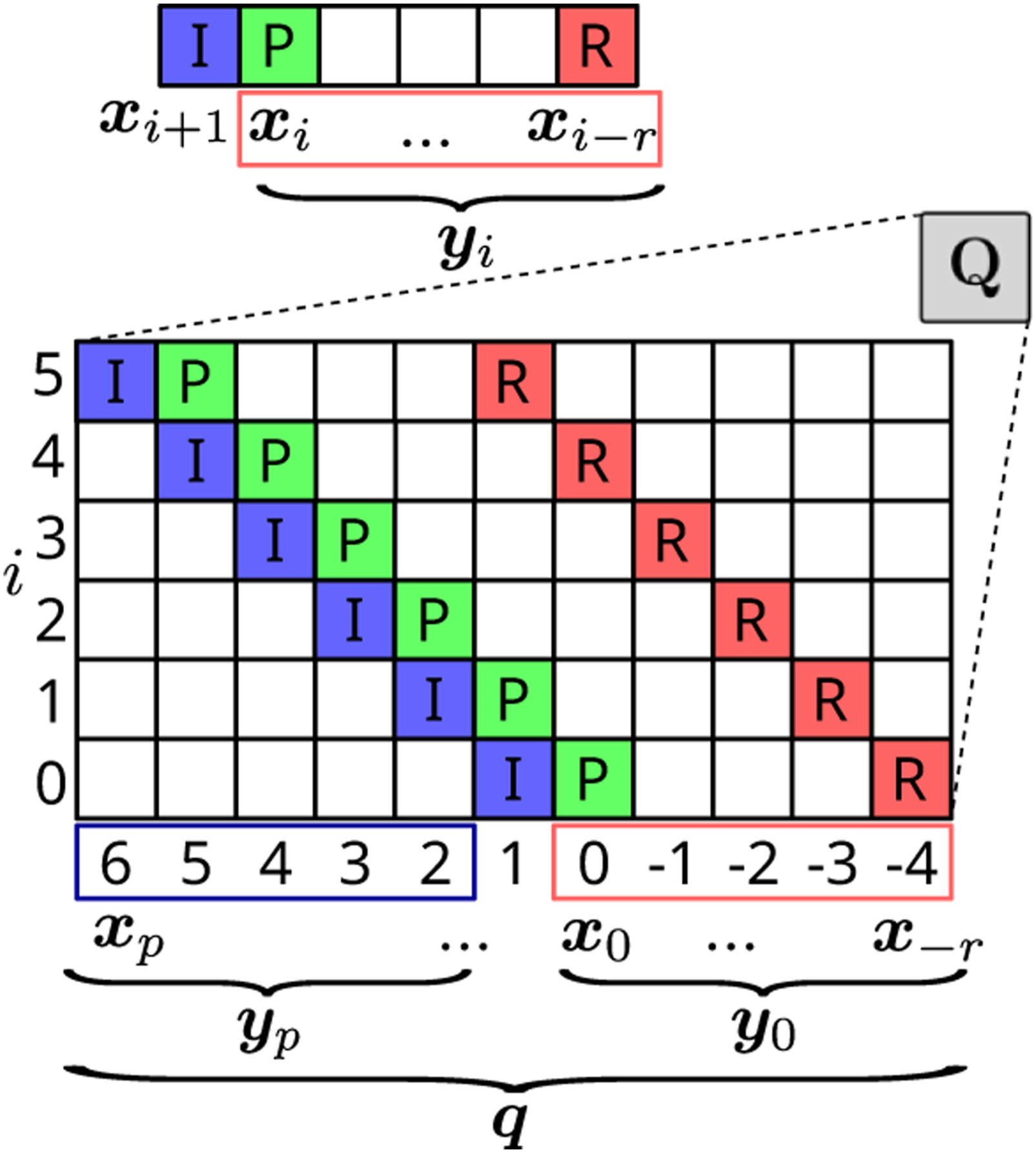

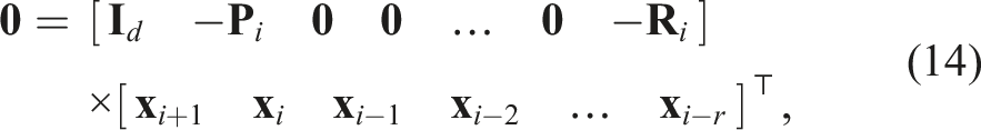
Repeating (14) for each index i ∈ 0, 1, …p − 1 yields the discretised

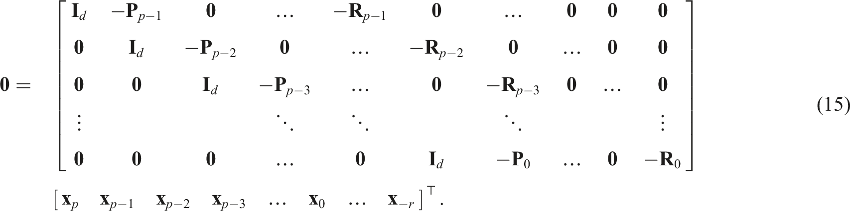
\begin{aligned} 0 = & [\begin{matrix} I_{d} & - P_{p - 1} & 0 & \dots & - R_{p - 1} & 0 & \dots & 0 & 0 & 0 \\ 0 & I_{d} & - P_{p - 2} & 0 & \dots & - R_{p - 2} & 0 & \dots & 0 & 0 \\ 0 & 0 & I_{d} & - P_{p - 3} & \dots & 0 & - R_{p - 3} & 0 & \dots & 0 \\ ⋮ & ⋱ & ⋱ & ⋱ & ⋮ \\ 0 & 0 & 0 & \dots & 0 & I_{d} & - P_{0} & \dots & 0 & - R_{0} \end{matrix}] \\ {[\begin{matrix} x_{p} & x_{p - 1} & x_{p - 2} & x_{p - 3} & \dots & x_{0} & \dots & x_{- r} \end{matrix}]}^{⊤} . \end{aligned}

(15)

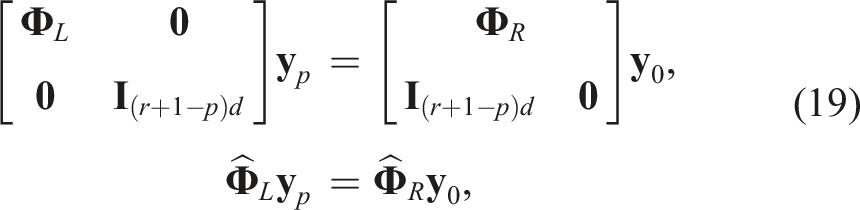
Note that the vector containing the discredited states from x_−r to x_p now covers the time interval t ∈ [t − τ, t + T]. This extended state vector will be denoted by q and the corresponding matrix coefficient by Q. The bottom section of Figure 2 shows the sketch of this composite description, with the coloured table depicting the matrix structure that emerges according to equation (15).

The goal of the spectral analysis is to perform a mapping of the state-space one period later. Therefore, the extended state vector needs to be split into two components that correspond to y_p and y₀. However, the period T and the time delay τ are only equal in special cases, thus, the resolutions p and r are usually not equal. The following sections discuss the cases where p − 1 = r, p − 1 > r and p − 1 < r. The schematic representations of these cases are shown in Figure 3.

Figure 3.

Schematic representation of the aggregated matrix structure for different p and r values. (left) p − 1 = r, (middle) p − 1 > r and (right) p − 1 < r. 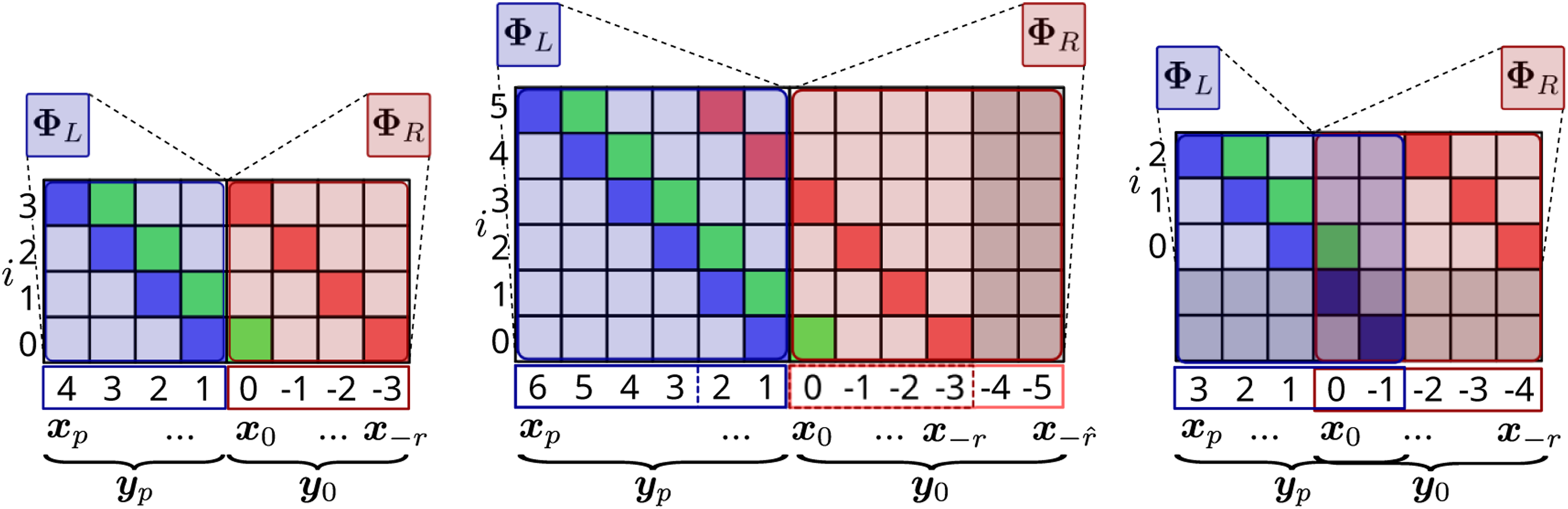$\hat{r}$ represents the extended states (see: Subsection partitioning of the equations for p − 1 < r). Red and blue rectangles represent the collections of states that belong to the initial and final sampled state space, respectively. Grey regions show the necessary extension to generate square left and right mapping matrices.

4.1. Partitioning of the equations for p − 1 = r

In this case, all the necessary elements of the sampled vector y_p and y₀ is found in the extended state vector q without overlap or missing elements (see Figure 3 left). Therefore, equation (15) can be separated into two components:

\begin{aligned} 0 = & [\begin{matrix} I_{d} & - P_{p - 1} & 0 & \dots & 0 & 0 & \dots & 0 \\ 0 & I_{d} & - P_{p - 2} & 0 & \dots & 0 & \dots & 0 \\ 0 & 0 & I_{d} & - P_{p - 3} & \dots & 0 \\ ⋮ & ⋱ & ⋱ & ⋮ \\ 0 & 0 & 0 & \dots & 0 & I_{d} & - P_{1} \\ 0 & 0 & 0 & \dots & 0 & \dots & I_{d} \end{matrix}] \\ {[\begin{matrix} x_{p} & x_{p - 1} & x_{p - 2} & x_{i - 2} & \dots & x_{1} \end{matrix}]}^{⊤} + \\ [\begin{matrix} - R_{p} & 0 & 0 & \dots & 0 & 0 & \dots & 0 \\ 0 & - R_{p - 1} & 0 & 0 & \dots & 0 & \dots & 0 \\ 0 & 0 & - R_{p - 1} & 0 & \dots & 0 \\ ⋮ & ⋱ & ⋱ & ⋮ \\ 0 & 0 & 0 & \dots & 0 & - R_{1} & 0 \\ - P_{0} & 0 & 0 & \dots & 0 & \dots & - R_{0} \end{matrix}] \\ {[\begin{matrix} x_{0} & \dots & x_{- 1} & \dots & x_{- r} \end{matrix}]}^{⊤}, \end{aligned}

(16)

where rearranging the equation yields

Φ_{L} y_{p} = Φ_{R} y_{0} .

(17)

The partitioned ‘left’ component of Q is denoted by Φ_L, while the negative of the ‘right’ component is denoted by Φ_R. The monodromy matrix Φ can be found by $Φ = Φ_{L}^{- 1} Φ_{R}$ .

However, in softwares specialised for numeric computations (e.g. Matlab, Julia), there is an option to compute the eigenvalues of $Φ = Φ_{L}^{- 1} Φ_{R}$ via a generalised eigenvalue calculation function based on Φ_R and Φ_L, avoiding the matrix inversion. This results in the same eigenvalues and eigenvectors (disregarding the numerical errors) as the original equation (7). Because Φ_L essentially has identity matrices on its block diagonal (due to the I terms in the left-hand side of the step-wise mapping), it is typically very well-conditioned, making the solution of the linear system Φ_Lx = b (which is what iterative solvers do internally instead of explicitly forming $Φ_{L}^{- 1} Φ_{R}$ ) numerically stable. The iterative solver evaluates the action of $Φ_{L}^{- 1} Φ_{R}$ on a vector, and the sparsity pattern of Φ_L allows this to be computed using highly efficient sparse forward/backward substitutions. Therefore, the overall conditioning and the convergence rate of the eigenvalue solver remain comparable to the traditional SD method, while the cost per iteration is vastly reduced.

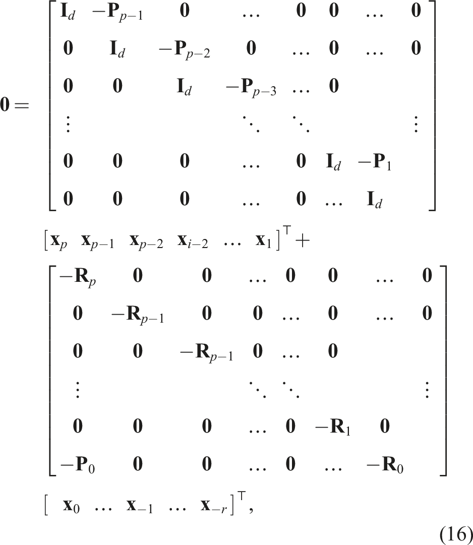
Note, that constructing the sparse Φ_L, $Φ_{R} \in R^{p d \times p d}$ matrix with a banded structure has linear time complexity and can be directly built after the computation of the submatrices P_i and R_i.

4.2. Partitioning of the equations for p − 1 > r

If the time period of the system is larger than the time delay T > τ, then p − 1 > r. In this case, the extended state vector q can be split into two separate vectors y_p and y₀. However, y_p and y₀ do not capture the intermediate states x_i: i ∈ {p − 1 − r, …, 2, 1}, and the corresponding equations. To remedy this, the value r should be updated to $\hat{r} = p - 1$ , as this choice still satisfies the inequality (3). With this choice, there are more points to store, and at the corresponding locations in the matrix Q of equation (15) must be padded with zeros (see the grey columns in the middle panel of the schematic representation in Figure 3). With these considerations, the partitioned representation of the system of equations is

\begin{aligned} 0 = & [\begin{matrix} I_{d} & - P_{p - 1} & 0 & \dots & - R_{p - 1} & 0 & \dots & 0 \\ 0 & I_{d} & - P_{p - 2} & 0 & \dots & - R_{p - 2} & \dots & 0 \\ 0 & 0 & I_{d} & - P_{p - 3} & \dots & 0 \\ ⋮ & ⋱ & ⋱ & ⋮ \\ 0 & 0 & 0 & \dots & 0 & I_{d} & - P_{1} \\ 0 & 0 & 0 & \dots & 0 & \dots & I_{d} \end{matrix}] \\ {[\begin{matrix} x_{p} & x_{p - 1} & x_{p - 2} & x_{i - 2} & \dots & x_{1} \end{matrix}]}^{⊤} + \\ [\begin{matrix} 0 & \dots & 0 & 0 & 0 & \dots & 0 \\ ⋮ & ⋮ & ⋮ \\ - R_{r} & 0 & 0 & 0 & \dots & 0 \\ ⋮ & ⋱ & ⋮ \\ 0 & \dots & - R_{1} & 0 & 0 & \dots & 0 \\ - P_{0} & \dots & 0 & - R_{0} & 0 & \dots & 0 \end{matrix}] \\ {[\begin{matrix} x_{0} & \dots & x_{- 1} & \dots & x_{- (p - 1)} \end{matrix}]}^{⊤} . \end{aligned}

(18)

Although we use more states than the original method requires, thus $Φ_{L}, Φ_{R} \in R^{(\hat{r} + 1) d \times (\hat{r} + 1) d} = R^{p d \times p d}$ which might initially seem to lead to higher computational time if T ≫ τ. However, in sparse representation, the zero padding in the matrix Q is ‘free’. As we will quantitatively demonstrate in Section 4 (where ratios of T/τ = 0.1, 1, and 10 are tested), the combined CPU time exhibits almost no difference between the cases where T/τ = 1 and T/τ = 10. Even for T/τ = 0.1, the total computation time remains practically identical. Therefore, the linear time complexity of the algorithm results in vastly more efficient computations than the original algorithm across a wide range of practical parameters.

Note that expanding the state vector y₀ to store more historical points than the original delay τ requires does not alter the dynamics of the discretized system, nor does it introduce spurious numerical modes. The additional points are simply used to ‘store’ the data for internal points. If T > τ, the state in [−τ, 0] does not fully describe the time-periodic solution; it merely serves as the initial state necessary for a simulation to eventually provide the periodic solution. With this expanded state vector, the full periodic solution over T is provided directly. Due to the sparse matrix structure, this extended capacity comes for ‘free’ without increasing the CPU time.

4.3. Partitioning of the equations for p − 1 < r

If T < τ and p − 1 < r, then there is an overlap between the y_p and y₀ (right panel of Figure 3). In this case, the nonzero elements of matrix Q corresponding to the overlapping elements in y_p and y₀ are free to be assigned to either Φ_L or Φ_R, a decision not influencing the end result. In this work, the coefficient matrix Q in equation (15) is partitioned as follows: the left side of matrix Q goes into $Φ_{L} \in R^{p d \times p d}$ , chosen to be a square matrix, while the remaining elements go into to $Φ_{R} \in R^{p d \times (r + 1) d}$ chosen to be rectangular (see the Figure 3). Finally, the corresponding system of equations must be completed by identity matrices that account for the equality of the overlapping elements, resulting in the system:

\begin{aligned} [\begin{matrix} Φ_{L} & 0 \\ 0 & I_{(r + 1 - p) d} \end{matrix}] y_{p} & = [\begin{matrix} Φ_{R} \\ I_{(r + 1 - p) d} 0 \end{matrix}] y_{0}, \\ {\hat{Φ}}_{L} y_{p} & = {\hat{Φ}}_{R} y_{0}, \end{aligned}

(19)

where I_(r+1−p)d is the identity matrix

\in R^{(r + 1 - p) d \times (r + 1 - p) d}

, thus both

{\hat{Φ}}_{L}

and

{\hat{Φ}}_{R} \in R^{(r + 1) d \times (r + 1) d}

4.4. Comptuation of the periodic solution

In many cases, the investigated system has periodic external forcing:

\dot{x} (t) = A (t) x (t) + B (t) x (t - τ) + c (t),

(20)

where c(t) = c (t + T), which leads to a non-zero periodic solution. Then applying the semi-discretization yields the affine map

x_{i + 1} = P_{i} x_{i} + R_{i} x_{i - r} + v_{i} i \in 0,1, \dots, p - 1,

(21)

see the definition of v_i in Insperger and Stépán (2011). The corresponding multiplication-free scheme is

Φ_{L} y_{p} = Φ_{R} y_{0} + V,

(22)

where

V = {[\begin{matrix} - v_{p - 1} & - v_{p - 2} & \dots & - v_{0} \end{matrix}]}^{⊤}

. Note that in the case when p − 1 < r, the vector V should be padded with zeros as well.

Then the discresited time-periodic solution will be the fixed point $\bar{y}$ of the map (22). Exploiting that $y_{p} = y_{0} = \bar{y}$ the fix point is given by

\bar{y} = {(Φ_{L} - Φ_{R})}^{- 1} V .

(23)

The stability of this fixed point can be determined based on the spectral radius ${\hat{Φ}}_{L}^{- 1} {\hat{Φ}}_{R}$ , as described previously.

The construction of the matrices Φ_L and Φ_R, along with the extended excitation vector V, involves a number of non-zero elements directly proportional to the resolution parameter p. This structural property implies not only linear CPU time for their generation but also linearly proportional memory usage when employing sparse matrix implementations. In contrast, the traditional monodromy matrix Φ typically evolves into a dense, almost full upper-triangular structure as it accumulates the effects of p recursive multiplications. Consequently, the memory requirement for the traditional approach scales quadratically $(O (p^{2}))$ . While this quadratic consumption is often manageable for standard engineering resolutions, it becomes a definitive bottleneck in high-accuracy scenarios. The MFSD method remains superior in these regimes, as its linear memory scaling enables the exploration of extremely high resolutions (e.g. p = 10⁶) that are practically impossible to test or store using traditional dense-matrix formulations.

Moreover, due to the special banded structure of these matrices, we anticipate that computing both the dominant Floquet multiplier and the periodic solution can be done with linear complexity when iterative methods such as Krylov subspace methods or Arnoldi iterations are utilised. These methods are particularly efficient for large, sparse matrices, as they construct solutions within Krylov subspaces, which reduces computational costs. These assumptions are substantiated by the numerical case studies presented in the subsequent section.

5. Numerical case studies

The introduced multiplication free semi-discretization method (MFSD) has been added to the SemiDiscretizationMethod.jl package², which is an efficient implementation of the Semi-Discretization method (Insperger and Stépán, 2011) in Bezanson et al. (2017). This package allows stability and periodic solution computations on time-periodic dynamical systems with multiple time delays and subjected to external forcing, even using higher-order semi-discretization methods. In the following sections, the computations were executed using these implementations, thus minimising the number of confounding factors when investigating algorithm performance and complexity.

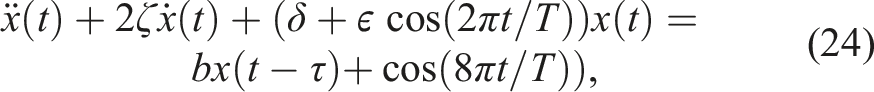
Note, we will analyse the CPU time only. Since the MFSD method is an exact algebraic rearrangement of the traditional SD mapping, the two methods are mathematically equivalent and MFSD introduces no new discretization errors. The numerical output of the built-in eigenvalue calculation (eigs with the default parameters) provides a numerically equivalent spectral radius. Throughout all the numerical results, the difference is bounded by floating-point round-off errors, that is, |μ_SD − μ_MFSD| < 3 × 10⁻¹⁵ for any parameter combination. Note that the convergence analysis for different order semi-discretizations is out of scope here, as it is discussed in detail in Insperger and Stépán (2011).

5.1. Delayed Mathieu equation with forcing

Common test cases for the validation of numerical methods for time-periodic DDEs are variations of the delayed Mathieu equation (Kovacic et al., 2018). Therefore, this section is dedicated to a variation of this model: the Mathieu Equation with a delayed state and subjected to external periodic forcing, which has the form of

\begin{aligned} \ddot{x} (t) + 2 ζ \dot{x} (t) + (δ + ϵ & \cos (2 π t / T)) x (t) = \\ b x (t - τ) + & \cos (8 π t / T)), \end{aligned}

(24)

where the time period of the parametric excitation is T.

We compare the MFSD method to the highly-optimised, open-source implementation of the traditional Semi-Discretization, which performs the successive matrix multiplication equation (7) based on sparse matrices and calculates the largest eigenvalues and the fixed point. The time measurements are based on the BenchmarkTools.jl, which performs multiple evaluations and provides the median and the standard deviation of the CPU time. The benchmark tests are stopped after 1000 evaluations or after 2 seconds, whichever comes first.

The variation of the measured evaluation times are also recorded, and are presented using the standard deviation with coloured areas for the cases where a sufficient number (>10) of evaluations was available. While the relative timing trends are of primary interest, for reproducibility, we specify the hardware configuration used in the tests: an Intel(R) Xeon(R) Gold 6154 CPU @ 3.00 GHz (36 cores) with 192 GB of RAM. All computations were performed using the Julia programming language and the SemiDiscretizationMethod.jl package. To numerically approximate the time complexity, a power function is fitted to the data for p > 100. In most cases, the fitted coefficients (the order of time complexity) are close to integer values; the small difference is related to the influence of the small p values and the fluctuation of the CPU time measurements.

In Figure 4(a), we plot the CPU time as a function of the discretization resolution p for each step listed in Section Time complexity of the semi-discretization method (note: p ∼ 1/Δt). As discussed previously, the construction of all the submatrices P_i and R_i, i = 1, 2, …, p has linear-time complexity $O (p^{1})$ , see the thin bright blue curve labelled as ‘SD-P_i, R_i- $O (p^{1.03})$ ’. The implementation of the C_i step matrix calculation is sub-optimal because each of them is stored separately, leading to quadratic time complexity $O (p^{2})$ (bright, thin red curve labelled as ‘SD-C_i- $O (p^{1.96})$ ’). This part is probably not optimised further in the original code because it is still one order of magnitude faster than the creation of the monodromy matrix Φ which has an almost cubic time complexity $O (p^{2.79})$ (bright, thin green curve labelled as ‘SD-Φ- $O (p^{2.79})$ ’) due to the dense structure of Φ. The last step of the spectral analysis is the calculation of the largest eigenvalue (μ₁), which is also much faster and has approximately quadratic time complexity (bright, thin magenta curve labelled as ‘SD-μ₁- $O (p^{1.69})$ ’). The CPU time of the fix point calculation is also tested: it has approximately quadratic time complexity $O (p^{2})$ (bright, thin pink curve labelled as ‘SD- $\bar{y}$ - $O (p^{2.08})$ ’). Figure 4(a) confirms the findings of Section Time complexity of the semi-discretization method, namely, that the bottleneck of the traditional semi-discretization method is the computation of the monodromy matrix with its complexity of $\sim O (p^{2.8})$ .

Figure 4.

Computation time of the traditional semi-discretization (SD) method (thin lines), and the multiplication free semi-discretization (MFSD) method (thick lines). The lines denote the mean values, and the coloured area denotes the corresponding ±1 standard deviation. Thin dashed black lines show the fitted curve. The parameters used during the tests are ζ = 0.2, δ = 3, ϵ = 3, b = −0.5, τ = 2π. (a); (b); and (c).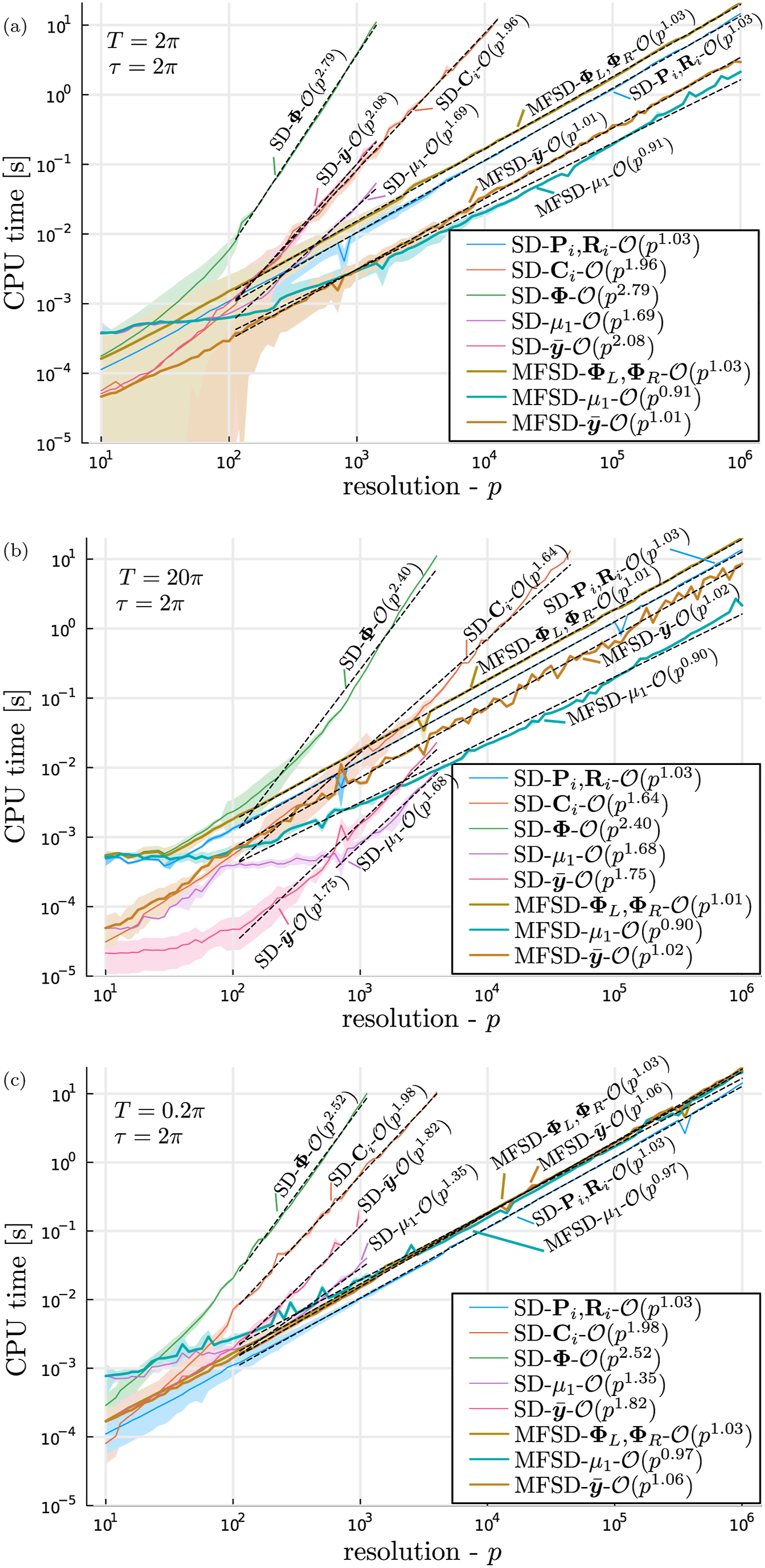

The CPU time of the MFSD method has four components. The first is identical to the computation of the P_i and R_i, which has linear-time complexity (thin bright blue curve labelled as ‘SD-P_i, R_i- $O (p^{1.03})$ ’, the same as in case of semi-discretization). The second is the construction of the Φ_L and Φ_R matrices. In this process, we create a sparse matrix from the previously computed submatrices and the identity matrices, which also have linear-time complexity (thick brown curve labelled as ‘MFSD-Φ_L, Φ_R- $O (p^{1.03})$ ’). The final (third) component of the stability analysis is the eigenvalue computation: in this case, the computation of the largest multiplier is faster than for the typically full upper triangular matrix Φ for SD, as it has linear-time complexity for the very sparse banded structure of the Φ_L and Φ_R matrices (see the thick green curve labelled as ‘MFSD-μ₁- $O (p^{0.91})$ ’). The computation complexity of fixed point calculation is also reduced to linear based on the numerical analysis (see the thick bright brown curve labelled as ‘MFSD- $\bar{y}$ - $O (p^{1.01})$ ’).

Figure 4(a) confirms that all the steps of the MFSD method have linear time complexity $O (p^{1})$ , and even for small p values, the computation time is similar to the original implementation. The figure also shows that we had to stop the CPU time measurement after around p ≈ 2000 for the original implementation of the SD method due to the computational demand. Still, in the case of the MFSD method, the CPU time measurements could be continued even for p = 10⁶.

Figures 4(b) and (c) compare the computation times for different T/τ ratios (10 and 0.1, respectively) to analyse the cases p > r and p < r discussed in Subsections Partitioning of the equations for p − 1 > r and Partitioning of the equations for p − 1 < r. The MFSD maintains linear time complexity, similarly to the case T = τ presented in Figure 4(a) because the number of P_i and R_i matrices is the same for a selected p value. The time complexity of the traditional SD method is also basically the same, with the worst being the time complexity $O (p^{2.4})$ – $O (p^{2.8})$ of computing the monodromy matrix Φ. However, there is a slight decrease in the complexity of some computation components due to the different density and non-zero element distribution of the Φ matrix.

Further numerical examples for different system sizes (different values of d) and multiple delays are provided in the Appendix. All cases exhibit similar trends in the graphs; the different CPU time relative to Figures 4(a)–(c) is attributed to the different number of nonzero elements in the system matrices.

All numerical tests support the fact that the Multiplication Free Semi-Discretization has a shorter CPU time for every p parameter and has linear time complexity, leading to orders of magnitude faster computations for scenarios where accurate results are critical.

6. Conclusion

The development and analysis of the multiplication free semi-discretization method (MFSD) presented in this study marks a significant advancement in numerical methods for delayed differential equations. The MFSD method is integrated into the existing open-source SemiDiscretization.jl Julia package, allowing the demonstration of the method’s superior computational efficiency through the excited Mathieu Equation. This study is driven by the hypothesis that it is possible to achieve linear time complexity in the numerical treatment of delayed dynamical systems, and the implemented MFSD showcases linear time complexity across different scenarios, including spectral analysis and calculation of time-periodic solution for systems with external excitation, making it a potent tool for handling complex dynamical systems with delay elements.

As the method maintains results in mapping matrices Φ_L and Φ_R with well-defined banded structures, it significantly reduces the computational time and resources necessary for the corresponding eigenvalue computations. This effect is especially prominent in cases where the traditional semi-discretization method exhibits quadratic or cubic time complexity.

The open-source implementation of the MFSD opens the way for the research community to make detailed calculations, where high resolution of the time period is essential to capture a system’s stability and steady-state behaviour accurately. This capability is particularly valuable in applications such as:

• Machine tool vibrations in milling processes: In milling operations, the regenerative effect introduces delays due to the periodic engagement of cutting teeth, leading to complex dynamics that can cause chatter. Accurate modelling of the stability and periodic motions of these systems is crucial for predicting and mitigating such instabilities (Kiss et al., 2022; Sanz-Calle et al., 2024; Ding et al., 2011).

• Networked control systems: In modern control systems, especially those distributed over networks, communication delays are inherent. These delays can significantly affect system stability and performance. Modelling and analysing these systems as time-delay systems help in designing robust controllers that can handle such delays effectively (Pan and Peng, 2024; Sun and Li, 2017).

• The semi-discretization method continues to be actively utilised as a robust tool for stability analysis in complex recent mechanical engineering applications (Kumar et al., 2025).

• Biological systems: delays often represent gestation or maturation periods. For example, in population dynamics, the reproduction rate at a given time may depend on the population size at an earlier time. Additionally, these models can exhibit time-periodic behaviour as a result of environmental cycles such as day/night rhythms or seasonal changes. Modelling these systems with delay differential equations allows for a more accurate representation of the biological processes involved (Smith, 2011; Arino et al., 2007).

• Traffic systems: Delays are inherent due to driver reaction times, which can lead to complex dynamics such as stop-and-go waves and phantom traffic jams. These phenomena have been effectively modelled using DDES (Molnar and Orosz, 2024; Martinovich et al., 2025). Moreover, traffic systems often exhibit time-periodic behaviour due to factors such as traffic light cycles and daily commuting patterns. Modelling these periodicities is crucial for understanding and optimising traffic flow (Jiang et al., 2024; Bartfai et al., 2024).

These examples illustrate the broad applicability of the MFSD method in accurately capturing the dynamics of systems where delays and periodicity play a critical role.

In future work, the MFSD method will be extended to distributed delays; however, the linear time complexity of the MFSD method is expected to degrade. When addressing systems with distributed delays, the number of elements – and consequently the computational time – can increase quadratically with the discretization parameter p. However, in the case of distributed delays, the traditional implementation is also expected to exhibit a similar degradation in computational complexity, transitioning to a higher time complexity (e.g. from $O (p^{2.8})$ to $O (p^{3.8})$ ). However, a detailed analysis of this behaviour is beyond the scope of the present work and is suggested as a direction for future research.

While the current formulation of the MFSD method is tailored for retarded delay differential equations, extending its applicability to neutral and advanced types – based on the work presented in Bartfai et al. (2023) – is a promising direction for future research. This extension is compatible with the proposed MFSD method, so implementing it in the SemiDiscretization.jl package would be a straightforward step. However, integrating this approach into the Julia framework would necessitate additional inputs and structural modifications within the package, which would require considerable implementation effort. Therefore, this task is left for a future project.

The MFSD approach has the potential to generalise well to the stochastic semi-discretization method (Sykora and Bachrathy, 2020), for which the actual quartic time complexity $(O (p^{4}))$ could be reduced to quadratic $(O (p^{2}))$ . In stochastic cases, handling the matrix D_i is crucial (see equations (9) and (10)); based on the further refinement of the MFSD, the constant improvement of (c/d)² could greatly improve the computational time. However, these method extensions are beyond this paper’s scope.

Furthermore, it is important to emphasise that the steps of the MFSD method are similar for the higher-order variations of the semi-discretization method, therefore resulting in similar performance.

Footnotes

Acknowledgements

We thank Henrik Sykora for creating the original implementation of the SemiDiscretization.jl package and for allowing me to access and enhance it.

ORCID iD

Daniel Bachrathy

Funding

The authors disclosed receipt of the following financial support for the research, authorship, and/or publication of this article: The research leading to these results was supported by the Hungarian Scientific Research Fund (NKFIH 138500 and NKFIH-152125).

Declaration of conflicting interests

The authors declared no potential conflicts of interest with respect to the research, authorship, and/or publication of this article.

Notes

Appendix

This appendix presents three practical test cases from the literature, of increasing complexity, on which timing results are reported.

Appendix A introduces a minimal population model with seasonal effects: a first-order DDE featuring constant maturation delay, time-periodic mortality and recruitment rates, and external forcing.

The second example, in Appendix B, involves a two-degree-of-freedom turning system with two distinct time-periodic delays, inspired by a practical application: a parallel cutting configuration combined with spindle-speed variation.

The third example, in Appendix B, models the longitudinal vibration of a beam with delayed boundary feedback, discretised using finite element methods. This case represents a high-dimensional system with constant delay and time-periodic excitation.

Note that the aim of the appendix is not to derive detailed models or analyse system behaviour in depth, but rather to present CPU time results across models of varying size and structure using the proposed MFSD method. We refer readers to the cited literature for complete model formulations and theoretical background.

References

Albertelli

Musletti

Leonesio

, et al. (2012) Spindle speed variation in turning: technological effectiveness and applicability to real industrial cases. The International Journal of Advanced Manufacturing Technology 62(1): 59–67. https://doi.org/10.1007/s00170-011-3790-8

Ali

Hou

Noori

(1998) Stability and performance of feedback control systems with time delays. Computers and Structures 66(2): 241–248. https://doi.org/10.1016/S0045-7949(97)00061-8

Arino

Hbid

Dads

(2007) Delay differential equations and applications. In: Proceedings of the NATO Advanced Study Institute Held in Marrakech. Springer Science & Business Media.

Åström

Murray

(2021) Feedback Systems: An Introduction for Scientists and Engineers. Princeton university press.

Bachrathy

Stepan

(2013) Improved prediction of stability lobes with extended multi frequency solution. CIRP Annals 62(1): 411–414. https://doi.org/10.1016/j.cirp.2013.03.085

Bartfai

Barrios

Dombovari

(2023) Stability Analysis of a One Degree of Freedom Robot Model With Sampled Digital Acceleration Feedback Controller in Turning and Milling. Journal of Computational and Nonlinear Dynamics. American Society of Mechanical Engineers, 18(8), 081011.

Bartfai

Dombovari

(2022) Hopf bifurcation calculation in neutral delay differential equations: nonlinear robotic arms subject to delayed acceleration feedback control. International Journal of Non-linear Mechanics 147: 104239. https://doi.org/10.1016/j.ijnonlinmec.2022.104239

Bartfai

Voros

Takacs

(2024) Stability analysis of a digital hierarchical steering controller of autonomous vehicles with multiple time delays. Journal of Vibration and Control 30(1-2): 330–341. https://doi.org/10.1177/10775463221146624

Bayly

Halley

Mann

, et al. (2003) Stability of interrupted cutting by temporal finite element analysis. J. Manuf. Sci. Eng 125(2): 220–225. https://doi.org/10.1115/1.1556860

10.

Bezanson

Edelman

Karpinski

, et al. (2017) Julia: a fresh approach to numerical computing. SIAM Review 59(1): 65–98. https://doi.org/10.1137/141000671

11.

Borgioli

Hajdu

Insperger

, et al. (2020) Pseudospectral method for assessing stability robustness for linear time-periodic delayed dynamical systems. International Journal for Numerical Methods in Engineering 121(16): 3505–3528. https://doi.org/10.1002/nme.6368

12.

Breda

Maset

Vermiglio

(2005) Pseudospectral differencing methods for characteristic roots of delay differential equations. SIAM Journal on Scientific Computing 27(2): 482–495. https://doi.org/10.1137/030601600

13.

Butcher

Bobrenkov

(2011) On the Chebyshev spectral continuous time approximation for constant and periodic delay differential equations. Communications in Nonlinear Science and Numerical Simulation 16(3): 1541–1554. https://doi.org/10.1016/j.cnsns.2010.05.037

14.

Ding

Zhu

Zhang

, et al. (2011) Milling stability analysis using the spectral method. Science China Technological Sciences 54: 3130–3136. https://doi.org/10.1007/s11431-011-4611-x

15.

Habib

Rega

Stepan

(2016) Delayed digital position control of a single-dof system and the nonlinear behavior of the act-and-wait controller. Journal of Vibration and Control 22(2): 481–495. https://doi.org/10.1177/1077546314533583

16.

Hamann

Eberhard

(2018) Stability analysis of milling processes with varying workpiece dynamics. Multibody System Dynamics 42: 383–396. https://doi.org/10.1007/s11044-017-9604-5

17.

Henninger

Eberhard

(2008) Improving the computational efficiency and accuracy of the semi-discretization method for periodic delay-differential equations. European Journal of Mechanics - A/Solids 27(6): 975–985. https://doi.org/10.1016/j.euromechsol.2008.01.006

18.

Horvath

Takacs

(2023) Balancing riderless electric scooters at zero speed in the presence of feedback delay. Multibody System Dynamics.

19.

Insperger

(2006) Act-and-wait concept for continuous-time control systems with feedback delay. IEEE Transactions on Control Systems Technology 14(5): 974–977. https://doi.org/10.1109/tcst.2006.876938

20.

Insperger

(2010) Full-discretization and semi-discretization for milling stability prediction: some comments. International Journal of Machine Tools and Manufacture 50(7): 658–662. https://doi.org/10.1016/j.ijmachtools.2010.03.010

21.

Insperger

Stépán

(2002) Semi-discretization method for delayed systems. International Journal for Numerical Methods in Engineering 55(5): 503–518. https://doi.org/10.1002/nme.505

22.

Insperger

Stepan

(2004) Stability analysis of turning with periodic spindle speed modulation via semidiscretization. Journal of Vibration and Control 10(12): 1835–1855. https://doi.org/10.1177/1077546304044891

23.

Insperger

Stépán

(2011) Semi-Discretization for Time-Delay Systems, Applied Mathematical Sciences. Springer New York, Vol. 178. https://doi.org/10.1007/978-1-4614-0335-7

24.

Insperger

Stépán

Turi

(2008) On the higher-order semi-discretizations for periodic delayed systems. Journal of Sound and Vibration 313(1-2): 334–341. https://doi.org/10.1016/j.jsv.2007.11.040

25.

Insperger

Stépán

Milton

(2022) Dynamics of human balancing. In: Controlling Delayed Dynamics: Advances in Theory, Methods and Applications. Springer, pp. 343–364.

26.

Itovich

Gentile

Moiola

(2024) Stability and bifurcations in time-delay systems: a novel and efficient blend of methods. International Journal of Bifurcation and Chaos 34(15): 2450195. https://doi.org/10.1142/s0218127424501955

27.

Jiang

Gan

Vörös

, et al. (2024) Safety filter for lane-keeping control. In: 16th International Symposium on Advanced Vehicle Control: Proceedings of AVEC’24–Society of Automotive Engineers of Japan. Springer Nature, pp. 371.

28.

Kiss

Hajdu

Bachrathy

, et al. (2022) In-process impulse response of milling to identify stability properties by signal processing. Journal of Sound and Vibration 527: 116849. https://doi.org/10.1016/j.jsv.2022.116849

29.

Kovacic

Rand

Mohamed Sah

(2018) Mathieu’s equation and its generalizations: overview of stability charts and their features. Applied Mechanics Reviews 70(2): 020802. https://doi.org/10.1115/1.4039144

30.

Kovacs

Insperger

(2018) Retarded, neutral and advanced differential equation models for balancing using an accelerometer. International Journal of Dynamics and Control 6: 694–706. https://doi.org/10.1007/s40435-017-0331-9

31.

Kumar

Prasad

Mitra

, et al. (2025) Delayed feedback control of pitch oscillations of an alp tower. International Journal of Mechanical Sciences 302: 110578. https://doi.org/10.1016/j.ijmecsci.2025.110578

32.

Le Gall

(2014) Powers of tensors and fast matrix multiplication. In: Proceedings of the 39th International Symposium on Symbolic and Algebraic Computation, (pp. 296–303). Association for Computing Machinery.

33.

Lehotzky

Insperger

(2016) A pseudospectral tau approximation for time delay systems and its comparison with other weighted-residual-type methods. International Journal for Numerical Methods in Engineering 108(6): 588–613. https://doi.org/10.1002/nme.5225

34.

Lehotzky

Insperger

Stepan

(2016) Extension of the spectral element method for stability analysis of time-periodic delay-differential equations with multiple and distributed delays. Communications in Nonlinear Science and Numerical Simulation 35: 177–189. https://doi.org/10.1016/j.cnsns.2015.11.007

35.

Lehotzky

Insperger

Stepan

(2018) Numerical methods for the stability of time-periodic hybrid time-delay systems with applications. Applied Mathematical Modelling 57: 142–162. https://doi.org/10.1016/j.apm.2017.12.029

36.

Gan

Cui

, et al. (2024) Potential field-based modeling and stability analysis of heterogeneous traffic flow. Applied Mathematical Modelling 125: 485–508. https://doi.org/10.1016/j.apm.2023.09.012

37.

Lichtner

Wolfrum

Yanchuk

(2011) The spectrum of delay differential equations with large delay. SIAM Journal on Mathematical Analysis 43(2): 788–802. https://doi.org/10.1137/090766796

38.

Liu

Tang

Chen

, et al. (2024) An efficient and precise stability analysis method for milling process. The International Journal of Advanced Manufacturing Technology 131: 1–16. https://doi.org/10.1007/s00170-024-13101-0

39.

Martin

Ruan

(2001) Predator-prey models with delay and prey harvesting. Journal of Mathematical Biology 43: 247–267. https://doi.org/10.1007/s002850100095

40.

Martinovich

Stepan

Bachrathy

, et al. (2025) Introducing state-dependent delay in the car-following model. Nonlinear Dynamics.

41.

Takács

Liu

, et al. (2024) Capturing the true bounding boxes: vehicle kinematic data extraction using unmanned aerial vehicles. Journal of Intelligent Transportation Systems 29: 1–13. https://doi.org/10.1080/15472450.2024.2341395

42.

Molnar

Orosz

(2024) Destroying phantom jams with connectivity and automation: nonlinear dynamics and control of mixed traffic. Transportation Science 58(6): 1319–1334. https://doi.org/10.1287/trsc.2023.0498

43.

Otto

Radons

(2013) Application of spindle speed variation for chatter suppression in turning. CIRP Journal of Manufacturing Science and Technology 6(2): 102–109. https://doi.org/10.1016/j.cirpj.2013.02.002

44.

Ozoegwu

(2018) A general order full-discretization algorithm for chatter avoidance in milling. Advances in Mechanical Engineering 10(7): 1687814018773811. https://doi.org/10.1177/1687814018773811

45.

Ozturk

Budak

(2008) Chatter stability of 5-axis milling using multi-frequency solution. In: Proceedings of the 3rd International Conference on High Performance Cutting, Dublin, Ireland, 7-9 July 2008, pp. 429–444.

46.

Pan

Peng

(2024) Finite region stability and networked predictive control for 2-d nonlinear time-delayed systems with quantization, packet dropouts and random disturbances. Systems & Control Letters 188: 105801. https://doi.org/10.1016/j.sysconle.2024.105801

47.

Reith

Bachrathy

Stepan

(2016) Improving the stability of multi-cutter turning with detuned dynamics. Machining Science and Technology 20(3): 440–459. https://doi.org/10.1080/10910344.2016.1191029

48.

Reith

Bachrathy

Stepan

(2017) Optimal detuning of a parallel turning system—theory and experiments. Journal of Dynamic Systems, Measurement, and Control 139(1): 014503. https://doi.org/10.1115/1.4034497

49.

Ruan

(2009) On nonlinear dynamics of predator-prey modelswith discrete delay. Mathematical Modelling of Natural Phenomena 4(2): 140–188. https://doi.org/10.1051/mmnp/2009009

50.

Saad

(2011) Numerical Methods for Large Eigenvalue Problems: Revised Edition. SIAM.

51.

Sanz-Calle

Munoa

Morelli

, et al. (2024) On the effect of radial engagement on the milling stability of modes perpendicular to the feed direction. CIRP Journal of Manufacturing Science and Technology 49: 111–127. https://doi.org/10.1016/j.cirpj.2024.01.006

52.

Smith

(2011) An Introduction to Delay Differential Equations with Applications to the Life Sciences. springer.

53.

Stepan

(2009) Delay effects in the human sensory system during balancing. Philosophical Transactions of the Royal Society A: Mathematical, Physical and Engineering Sciences 367(1891): 1195–1212. https://doi.org/10.1098/rsta.2008.0278

54.

Strassen

(1969) Gaussian elimination is not optimal. Numerische Mathematik 13(4): 354–356. https://doi.org/10.1007/bf02165411

55.

Sun

(2017) Synchronization transitions induced by partial time delay in a excitatory–inhibitory coupled neuronal network. Nonlinear Dynamics 89(4): 2509–2520. https://doi.org/10.1007/s11071-017-3600-4

56.

Sykora

Bachrathy

(2020) Stochastic semidiscretization method: second moment stability analysis of linear stochastic periodic dynamical systems with delays. Applied Mathematical Modelling 88: 933–950. https://doi.org/10.1016/j.apm.2020.06.078

57.

Szekrényes

(2023) Stability of delaminated composite beams subjected to retarded periodic follower force. Archive of Applied Mechanics 93(11): 4197–4216. https://doi.org/10.1007/s00419-023-02489-y

58.

Szekrényes

(2025) Mechanics of delaminated composite beams subjected to retarded follower force with multiple time delay. Acta Mechanica 236(2): 655–672. https://doi.org/10.1007/s00707-024-04161-0

59.

Toth

Bachrathy

Stepan

(2017) Effect of wavy tool path on the stability properties of milling by the implicit subspace iteration method. The International Journal of Advanced Manufacturing Technology 91: 1781–1789. https://doi.org/10.1007/s00170-016-9827-2

60.

Vyasarayani

Subhash

Kalmár-Nagy

(2014) Spectral approximations for characteristic roots of delay differential equations. International Journal of Dynamics and Control 2: 126–132. https://doi.org/10.1007/s40435-014-0060-2

61.

Yang

Yuan

Tie

, et al. (2023) An efficient and accurate chatter prediction method of milling processes with a transition matrix reduction scheme. Mechanical Systems and Signal Processing 182: 109535. https://doi.org/10.1016/j.ymssp.2022.109535

62.

Zatarain

Dombovari

(2014) Stability analysis of milling with irregular pitch tools by the implicit subspace iteration method. International Journal of Dynamics and Control 2: 26–34. https://doi.org/10.1007/s40435-013-0052-7

63.

Zatarain

Alvarez

Bediaga

, et al. (2015) Implicit subspace iteration as an efficient method to compute milling stability lobe diagrams. The International Journal of Advanced Manufacturing Technology 77: 597–607. https://doi.org/10.1007/s00170-014-6470-7

64.

Zhang

Stepan

(2016) Exact stability chart of an elastic beam subjected to delayed feedback. Journal of Sound and Vibration 367: 219–232. https://doi.org/10.1016/j.jsv.2016.01.002

65.

Zhang

(2022) Vibration control of a time-delayed rotor-active magnetic bearing system by time-varying stiffness. International Journal of Applied Mechanics 14(04): 2250007. https://doi.org/10.1142/s1758825122500077