Antiplane shear wave dynamics in functionally graded materials: A green’s function framework

Abstract

The present study investigates horizontally polarized shear wave propagation in an inhomogeneous, anisotropic medium with depth-dependent elastic properties. A Green’s function formulation is developed to characterize transient SH-waves in a transversely isotropic medium whose material parameters follow a power-law variation along the depth in a Cartesian coordinate system. In particular, the elastic modulus and mass density are prescribed through distinct power-function profiles, enabling independent control of inhomogeneity effects. Under these assumptions, Green’s functions corresponding to the governing inhomogeneous scalar wave equations are derived, and closed-form expressions for the displacement fields associated with the wavefronts are obtained. The singular points of the solution are identified in terms of the wave arrival times, and the onset of a secondary diffracted wave generated by the incoming front is highlighted. Numerical results illustrate the influence of the inhomogeneity parameters associated with the elastic moduli and density, demonstrating that certain parameter regimes lead to upward shifting of wavefronts, whereas others result in downward shifting, thereby highlighting the significant role of material grading on wave kinematics in anisotropic environments.

Keywords

Green’s function anisotropy SH-waves displacement inhomoegeneous solid scalar wave wavefronts

1. Introduction

Over the past several decades, the mathematical modeling of wave propagation in inhomogeneous and anisotropic solids has attracted renewed attention, motivated in large part by the expanding use of functionally graded, bio-inspired, and engineered materials in modern applications. These materials exhibit spatially varying elastic properties and enable mechanical responses that do not occur naturally, thereby necessitating sophisticated theoretical models for waves and fields in inhomogeneous continua, as discussed by Chew (1995), Payton (2012). Advances in fabrication have made such graded media—including quasi-incompressible plates and soft solids used in elastography-practically realizable, generating both new technological posibilities and new analytical challenges, as demonstrated by Benech et al. (2017, 2022).

The prime objective in this area is the construction of analytical solution and Green’s function for point or may be line source, that serve as the basic building blocks in direct modelling, inverse problems, and boundary integral formulations. Such solutions have been extensively employed in geophysical prospecting, structural dynamics, and layered half-space analysis by researchers including Chen and Cao (2020); Restrepo and Gómez (2014); Manolis and Karakostas (2003); Manolis and Shaw (1996). Their derivation requires sophisticated applications of integral transforms, special functions, and exact ordinary differential equation techniques. Classical references such as the transformation tables of Zaitsev and Polyanin (2002), the handbook of Oberhettinger and Badii (2012), the treatise of Bateman et al. (1954), the work of Sneddon (1972) continue to provide indispensable analytical tools for this purpose. Likewise, the theoretical frameworks developed by Debnath and Bhatta (2011); Morse and Feshbach (1953) remain central to the derivation and inversion of transform-domain representations. More recently, Singh et al. (2017), Kumhar et al. (2020), and Hemalatha et al. (2025) successfully employed Green’s function methodologies to rigorously investigate anti-plane wave propagation in inhomogeneous graded media under point-source excitation. Related developments in the study of wave dispersion and scattering in graded solids have been reported by Kumawat et al. (2025b), Chaudhary et al. (2025), and Panigrahi et al. (2025).

In modeling wave propagation in inhomogeneous media, SH waves are the most natural choice, since they offer a simpler framework than the coupled quasi P-SV waves while preserving the complexity associated with multidimensional propagation.

Exact closed-form solutions for multidimensional waves in inhomogeneous media remain relatively scarce. Among the earliest contribution, Hook (1962) derived a Green’s function describing wave propagation in axisymmetric, inhomogeneous and isotropic media. Subsequently, Watanabe (1982) presented important results for radially inhomogeneous elastic solids characterized by linearly varying wave velocities. Building upon these developments, Watanabe and Payton (2004) provided a more comprehensive collection of exact solutions for wave propagation in inhomogeneous isotropic media, including three Green’s functions governing transient and time-harmonic SH-waves as well as torsional waves. In their formulation, the SH-wave velocity was assumed to vary linearly with depth in a Cartesian coordinate system and according to a power-law function of the radial distance in a polar coordinate system.

The determination of exact solutions for point or line sources in anisotropic and inhomogeneous media is generally a challenging task. Rangelov et al. (2005) obtained time-harmonic fundamental solutions for a particular class of two-dimensional anisotropic and inhomogeneous media. Using a similar form of material inhomogeneity, Daros (2008, 2009) derived fundamental solutions for transient and time-harmonic anti-plane waves, together with time-harmonic in-plane waves in transversely isotropic media. A common restriction in the formulation of (Daros, 2008, 2009; Rangelov et al., 2005) was that the spatial variations of density and elastic stiffness were required to follow the same inhomogeneity profile, thereby limiting the range of material gradations that could be represented.

More recently, several researchers have investigated SH-wave propagation in complex media involving interfaces and microstructional effects. For example, Mistri et al. (2026) examined wave behavior in smart porous composites containing electrically induced interfaces. Using the framework of strain-gradient elasticity, Kumawat and Vishwakarma (2025a, 2025b) investigated reflection-transmission characteristics across membrane-spring layered interfaces using strain gradient theory. Furthermore, Kumawat et al. (2025a) highlighted dispersive effects in strain-gradient media under initial stress.

In contrast, the present work focuses on transient SH-wave propagation in continuously graded anisotropic media. By developing a Green’s function framework with independently varying material properties, it extends these studies from discrete interface and microstructural effects to smooth inhomogeneity, providing deeper insight into wavefront evolution and diffraction in graded materials.

The current work presents a novel approach in the development of an exact analytical method for transient SH-wave propagation in a transversely isotropic medium with independently varying elastic and inertial properties. While (Chen and Cao, 2020; Daros, 2013; Hemalatha et al., 2025; Kumhar et al., 2020; Watanabe and Payton, 1997) considered material models in which the density and stiffness coefficients were constrained to possess identical spatial inhomogeneitues profiles, the present formulation generalizes these assumptions by allowing independent power-law variation of the material parameters. Consequently, the propsoed model is capable of representing a broader and more realistic class of functionally graded materials. The closed-form representation of the displacement field is derived through a Green’s function methodology, a result that remains relatively rare in the literature on multidimentional anisotropic inhomogeneous media. Furthermore, the analysis explicitly identifies the singular structure of the solution in terms of wave-arival times and reveals the emergence of secondary diffracted wavefronts, thereby providing deeper physical insight into trasient wave phenomena. The results presented herein not only recover several classical solutions as limiting cases but also furnish a rigorous analytical benchmark for the validation of numerical and computational models in complex graded materials.

2. Governing equations and assumptions

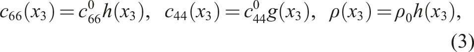
In the current study, the propagation of anti-plane SH waves in a functionally graded elastic medium is investigated using the Green’s function framework. The following assumptions are adopted for the formulation of the solution.

1. The medium is assumed to be an elastic anisotropic solid whose mechanical properties vary along the x₃ coordinate (depth). The elastic moduli c₄₄, c₆₆ and ρ depends on the coordinate x₃, which shows uneven nature of the solid.

2. The analysis is limited to anti-plane SH motion, where displacement field is directed along out-of-plane where wave propagates in in-plane coordinates.

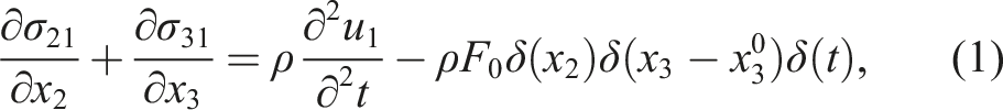
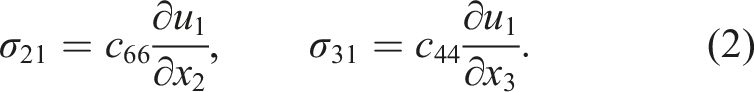
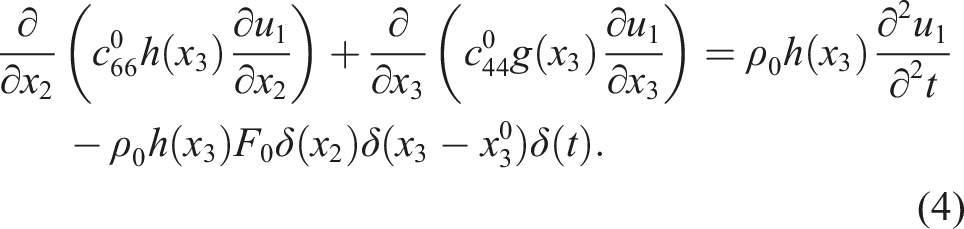
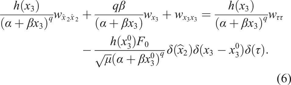
Consider a transversely isotropic solid in Cartesian coordinates (x₁, x₂, x₃) where the coordinate origin coincides with the center of anisotropy. For an anti-plane deformation, the governing equation of motion for an SH point (line) source (polarized in the x₁-direction and positioned at (x₂ = 0, x₃ = $x_{3}^{0}$ )) is given by

\frac{\partial σ_{21}}{\partial x_{2}} + \frac{\partial σ_{31}}{\partial x_{3}} = ρ \frac{\partial^{2} u_{1}}{\partial^{2} t} - ρ F_{0} δ (x_{2}) δ (x_{3} - x_{3}^{0}) δ (t),

(1)

where ρ is the density, δ(⋅) is the Dirac’s delta and F₀ is the magnitude source. The stress-strain relation is given by

σ_{21} = c_{66} \frac{\partial u_{1}}{\partial x_{2}}, σ_{31} = c_{44} \frac{\partial u_{1}}{\partial x_{3}} .

(2)

Here c₆₆ and c₄₄ are elastic moduli and ρ is mass density which is considered to vary along the depth x₃ by means of the gradation function h (x₃) and g (x₃), are given by

c_{66} (x_{3}) = c_{66}^{0} h (x_{3}), c_{44} (x_{3}) = c_{44}^{0} g (x_{3}), ρ (x_{3}) = ρ_{0} h (x_{3}),

(3)

where

c_{66}^{0}

c_{66}^{0}

, and ρ₀ are constants. We specifically relax the constraints imposed in Rangelov et al. (2005), and Daros (2008) by considering a different depth-dependent inhomogeneity profile for c₄₄(x₃). Using equations (1)–(3), we obtain the equation of motion in terms of the anti-plane displacement u₁ expressed as

\frac{\partial}{\partial x_{2}} (c_{66}^{0} h (x_{3}) \frac{\partial u_{1}}{\partial x_{2}}) + \frac{\partial}{\partial x_{3}} (c_{44}^{0} g (x_{3}) \frac{\partial u_{1}}{\partial x_{3}}) = ρ_{0} h (x_{3}) \frac{\partial^{2} u_{1}}{\partial^{2} t} - ρ_{0} h (x_{3}) F_{0} δ (x_{2}) δ (x_{3} - x_{3}^{0}) δ (t) .

(4)

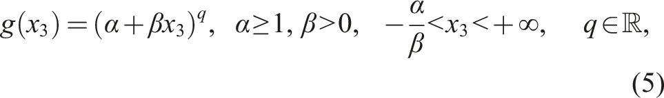
We now restrict the function g (x₃) to be a polynomial function as

g (x_{3}) = {(α + β x_{3})}^{q}, α \geq 1, β > 0, - \frac{α}{β} < x_{3} < + \infty, q \in R,

(5)

where α, β, and q are the inhomogeneity coefficients known as surface property parameter, gradation rate parameter, shape parameter, respectively. We introduce a new time coordinate

τ = \sqrt{c_{44}^{0}} t

and redefine displacement u₁ as

u_{1} = \sqrt{\frac{ρ_{0}}{c_{44}^{0}}} w

. Dividing (4) by c₄₄ (x₃), and introducing the dimensionless elastic stiffness ratio

μ = c_{66}^{0} / c_{44}^{0}

, we define a scaled spatial coordinate

{\hat{x}}_{2} = x_{2} / \sqrt{μ}

. With this transformation, (4) can be written in the following form:

\frac{h (x_{3})}{{(α + β x_{3})}^{q}} w_{{\hat{x}}_{2} {\hat{x}}_{2}} + \frac{q β}{(α + β x_{3})} w_{x_{3}} + w_{x_{3} x_{3}} = \frac{h (x_{3})}{{(α + β x_{3})}^{q}} w_{τ τ} - \frac{h (x_{3}^{0}) F_{0}}{\sqrt{μ} {(α + β x_{3}^{0})}^{q}} δ ({\hat{x}}_{2}) δ (x_{3} - x_{3}^{0}) δ (τ) .

(6)

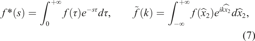
Using the Laplace and the Fourier transforms as defined below

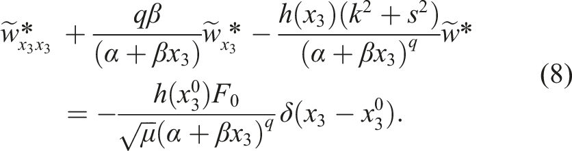
f^{*} (s) = \int_{0}^{+ \infty} f (τ) e^{- s τ} d τ, \tilde{f} (k) = \int_{- \infty}^{+ \infty} f ({\hat{x}}_{2}) e^{i k {\hat{x}}_{2}} d {\hat{x}}_{2},

(7)

We obtain the following expression

{\tilde{w}}_{x_{3} x_{3}}^{*} + \frac{q β}{(α + β x_{3})} {\tilde{w}}_{x_{3}}^{*} - \frac{h (x_{3}) (k^{2} + s^{2})}{{(α + β x_{3})}^{q}} {\tilde{w}}^{*} = - \frac{h (x_{3}^{0}) F_{0}}{\sqrt{μ} {(α + β x_{3})}^{q}} δ (x_{3} - x_{3}^{0}) .

(8)

Let us discuss the quadratic gradation by setting q = 2 and making use of the mapping ${\tilde{w}}^{*} (x_{3}) = {\tilde{w}}_{1}^{*} (x_{3}) / (α + β x_{3})$ , the homogeneous ODE associated with (8) reduces to the following wave equation.

{\tilde{w}}_{1, x_{3} x_{3}}^{*} + l^{2} m^{2} (x_{3}) {\tilde{w}}_{1}^{*} = 0, where m^{2} (x_{3}) = \frac{h (x_{3})}{{(α + β x_{3})}^{2}}, l^{2} = - (k^{2} + s^{2}) .

(9)

A second order ODE of the form A (x) d²y/dx² + B(x)dy/dx + C (x) y = 0 can be converted to the form d²w/dx² + P (x) w = 0 by using the mapping y (x) = w (x) μ (x) where $μ (x) = \exp (- 1 / 2 \int B (t) / A (t) d t)$ . However, we are searching for a class of ODEs whose solutions allow for the development of precise Green’s functions using inverse integral transforms. A closed form Green’s function corresponding to a class of anisotropic, inhomogeneous media is derived by using the mapping mentioned.

3. Green’s function for parabolic velocity profile

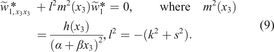
The objective is to identify the possible solutions of the reduced wave equation (9). Abraham and HE (1982) derived new solutions to the acoustic wave equation for certain velocity profiles by exploiting its relation to the Schrodinger equation.

The parabolic velocity profile provides an initial illustration of the derivation of a general Green’s function corresponding to a power-function velocity profile. Let us assume $h (x_{3}) = γ / {(α + β x_{3})}^{2}$ , where γ is a scaling factor parameter, then the solution to (9) becomes

{\tilde{w}}_{1}^{* H} = (α + β x_{3}) (c_{1} e^{- i \frac{k \sqrt{γ}}{β (α + β x_{3})}} + c_{2} e^{i \frac{k \sqrt{γ}}{β (α + β x_{3})}}),

(10)

where superscript H stands for homogeneous solution, c₁ and c₂ are arbitrary constants, and

i = \sqrt{- 1}

. Now returning back to

{\tilde{w}}^{*}

, we obtain

{\tilde{w}}^{* H} = c_{1} e^{\frac{- \sqrt{γ (k^{2} + s^{2})}}{β (α + β x_{3})}} + c_{2} e^{\frac{\sqrt{γ (k^{2} + s^{2})}}{β (α + β x_{3})}} .

(11)

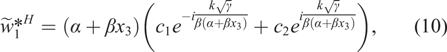
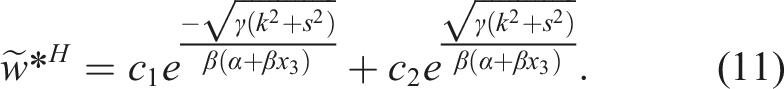
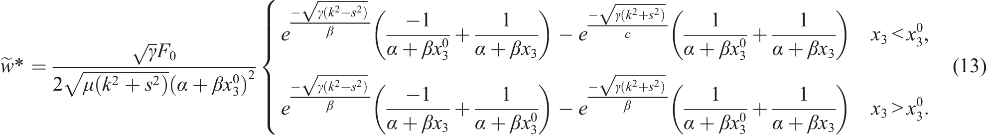
However, the linearly independent solutions obtained in (11) cannot be directly used to derive a point source representation, as they do not exhibit the decay of displacement values at the boundaries of the domain −α/β < x₃ < ∞.

As x₃ → −α/β the solution function multiplying c₁ satisfies the homogeneous boundary condition, but as x₃ → +∞ the solution function multiplying c₂ does not satisfy the homogeneous condition. Instead of these solutions, we can use a new set of linearly independent solutions of (9) as

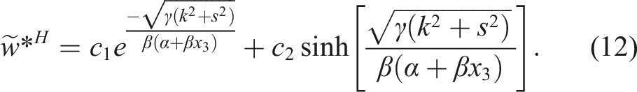
{\tilde{w}}^{* H} = c_{1} e^{\frac{- \sqrt{γ (k^{2} + s^{2})}}{β (α + β x_{3})}} + c_{2} \sinh [\frac{\sqrt{γ (k^{2} + s^{2})}}{β (α + β x_{3})}] .

(12)

By expressing Sinh [.] in terms e^x and e^−x (sinh x = e^x − e^−x/2) the Green’s function from (12) takes the form

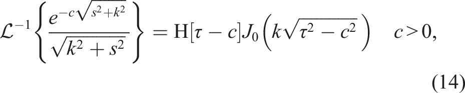
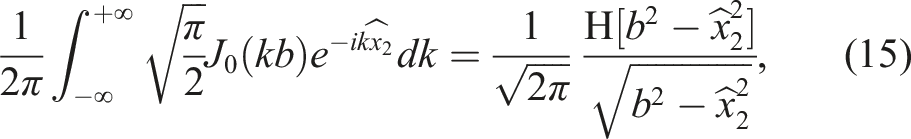
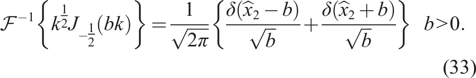
{\tilde{w}}^{*} = \frac{\sqrt{γ} F_{0}}{2 \sqrt{μ (k^{2} + s^{2})} {(α + β x_{3}^{0})}^{2}} \{\begin{cases} e^{\frac{- \sqrt{γ (k^{2} + s^{2})}}{β}} (\frac{- 1}{α + β x_{3}^{0}} + \frac{1}{α + β x_{3}}) - e^{\frac{- \sqrt{γ (k^{2} + s^{2})}}{c}} (\frac{1}{α + β x_{3}^{0}} + \frac{1}{α + β x_{3}}) x_{3} < x_{3}^{0}, \\ e^{\frac{- \sqrt{γ (k^{2} + s^{2})}}{β}} (\frac{- 1}{α + β x_{3}} + \frac{1}{α + β x_{3}^{0}}) - e^{\frac{- \sqrt{γ (k^{2} + s^{2})}}{β}} (\frac{1}{α + β x_{3}^{0}} + \frac{1}{α + β x_{3}}) x_{3} > x_{3}^{0} . \end{cases}

(13)

Applying inverse Laplace transform formula given by Oberhettinger and Badii (2012) followed by inverse Fourier transform formula as suggested in Sneddon (1972), we have

L^{- 1} \{\frac{e^{- c \sqrt{s^{2} + k^{2}}}}{\sqrt{k^{2} + s^{2}}}\} = H [τ - c] J_{0} (k \sqrt{τ^{2} - c^{2}}) c > 0,

(14)

\frac{1}{2 π} \int_{- \infty}^{+ \infty} \sqrt{\frac{π}{2}} J_{0} (k b) e^{- i k {\hat{x}}_{2}} d k = \frac{1}{\sqrt{2 π}} \frac{H [b^{2} - {\hat{x}}_{2}^{2}]}{\sqrt{b^{2} - {\hat{x}}_{2}^{2}}},

(15)

The final form of Green’s function is obtained as

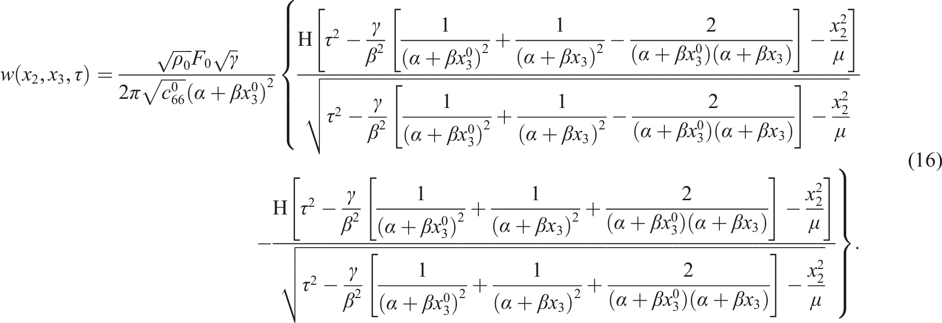
\begin{aligned} w (x_{2}, x_{3}, τ) = \frac{\sqrt{ρ_{0}} F_{0} \sqrt{γ}}{2 π \sqrt{c_{66}^{0}} {(α + β x_{3}^{0})}^{2}} \{\frac{H [τ^{2} - \frac{γ}{β^{2}} [\frac{1}{{(α + β x_{3}^{0})}^{2}} + \frac{1}{{(α + β x_{3})}^{2}} - \frac{2}{(α + β x_{3}^{0}) (α + β x_{3})}] - \frac{x_{2}^{2}}{μ}]}{\sqrt{τ^{2} - \frac{γ}{β^{2}} [\frac{1}{{(α + β x_{3}^{0})}^{2}} + \frac{1}{{(α + β x_{3})}^{2}} - \frac{2}{(α + β x_{3}^{0}) (α + β x_{3})}] - \frac{x_{2}^{2}}{μ}}} \\ - \frac{H [τ^{2} - \frac{γ}{β^{2}} [\frac{1}{{(α + β x_{3}^{0})}^{2}} + \frac{1}{{(α + β x_{3})}^{2}} + \frac{2}{(α + β x_{3}^{0}) (α + β x_{3})}] - \frac{x_{2}^{2}}{μ}]}{\sqrt{τ^{2} - \frac{γ}{β^{2}} [\frac{1}{{(α + β x_{3}^{0})}^{2}} + \frac{1}{{(α + β x_{3})}^{2}} + \frac{2}{(α + β x_{3}^{0}) (α + β x_{3})}] - \frac{x_{2}^{2}}{μ}}}\} . \end{aligned}

(16)

The following identity involving the product of Heaviside functions has been used in (16), which unifies the two Heaviside functions obtained after applying the Laplace transform followed by the Fourier transform to (13).

H [τ - p] H [τ^{2} - p^{2} - q^{2}] \equiv H [τ^{2} - p^{2} - q^{2}] q^{2} > 0 .

(17)

4. Green’s function for power-function velocity profile

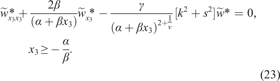
To generalize the analysis, we consider the Green’s function for a power-function velocity variation in the x₃-direction. We now turn to consideration of $h (x_{3}) = γ / {(α + β x_{3})}^{1 / ν}$ where $ν \in R$ . Introducing the substitutions ${\hat{x}}_{3} = α + β x_{3}$ , n = 2 + 1/ν and ω² = γ (k² + s²)/β² equation (9) is written as

{\tilde{w}}_{1, {\hat{x}}_{3} {\hat{x}}_{3}}^{*} - \frac{ω^{2}}{{\hat{x}}_{3}^{n}} {\tilde{w}}_{1}^{*} = 0 .

(18)

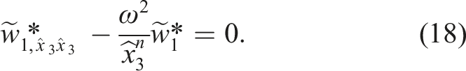
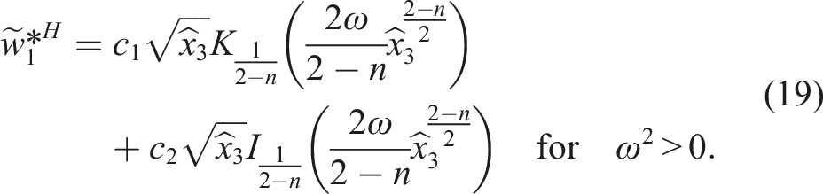
In Zaitsev and Polyanin (2002), a general solution for this equation can be found. For an arbitrary n, the solution can be expressed in terms of Bessel and modified Bessel functions. In the present discussion, we focus on the case ω² > 0 in which the solution involves modified Bessel functions that involve functions of the first and second kind.

{\tilde{w}}_{1}^{* H} = c_{1} \sqrt{{\hat{x}}_{3}} K_{\frac{1}{2 - n}} (\frac{2 ω}{2 - n} {\hat{x}}_{3}^{\frac{2 - n}{2}}) + c_{2} \sqrt{{\hat{x}}_{3}} I_{\frac{1}{2 - n}} (\frac{2 ω}{2 - n} {\hat{x}}_{3}^{\frac{2 - n}{2}}) for ω^{2} > 0 .

(19)

However, the solution is incompatible with homogeneous boundary conditions. To recover the Bessel equation, we introduce the substitutions ${\hat{w}}_{1}^{*} = y (\hat{x_{3}}) {\hat{x}}_{3}^{1 / 2}$ , $ξ = ν {(1 / {\hat{x}}_{3})}^{(1 / 2 ν)}$ and define the mapping $Φ (ξ) = y ({\hat{x}}_{3} (ξ))$ in (18), which yields the following.

\frac{1}{4} {(\frac{ξ}{ν})}^{4 ν + 2} [\frac{d^{2} Φ}{d ξ^{2}} + \frac{1}{ξ} \frac{d Φ}{d ξ} - (\frac{ν^{2}}{ξ^{2}} + 4 λ^{2}) Φ] = 0 .

(20)

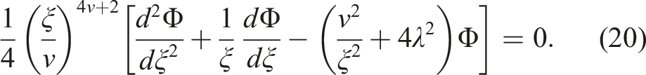
Therefore, the solution for (20) is obtained as follows.

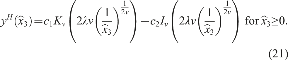
y^{H} ({\hat{x}}_{3}) = c_{1} K_{ν} (2 λ ν {(\frac{1}{{\hat{x}}_{3}})}^{\frac{1}{2 ν}}) + c_{2} I_{ν} (2 λ ν {(\frac{1}{{\hat{x}}_{3}})}^{\frac{1}{2 ν}}) for {\hat{x}}_{3} \geq 0 .

(21)

Afterward returning to x₃ and ${\tilde{w}}^{*} (x_{3})$ we obtain

{\tilde{w}}^{* H} (x_{3}) = c_{1} \frac{1}{\sqrt{α + β x_{3}}} K_{ν} (\frac{2 ν}{β} \sqrt{γ (k^{2} + s^{2})} {(\frac{1}{α + β x_{3}})}^{\frac{1}{2 ν}}) + c_{2} \frac{1}{\sqrt{α + β x_{3}}} I_{ν} (\frac{2 ν}{β} \sqrt{γ (k^{2} + s^{2})} {(\frac{1}{α + β x_{3}})}^{\frac{1}{2 ν}}),

(22)

as a solution to

{\tilde{w}}_{x_{3} x_{3}}^{*} + \frac{2 β}{(α + β x_{3})} {\tilde{w}}_{x_{3}}^{*} - \frac{γ}{{(α + β x_{3})}^{2 + \frac{1}{ν}}} [k^{2} + s^{2}] {\tilde{w}}^{*} = 0, x_{3} \geq - \frac{α}{β} .

(23)

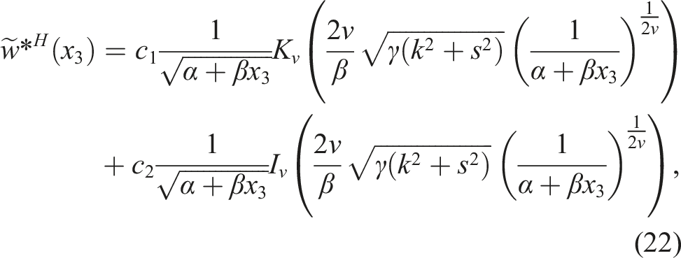
However, the set of solutions in (22) is only applicable to ν > 0. For ν ≤ 0, the homogeneous boundary conditions are not satisfied. As a result, we believe that we have discovered a restriction regarding the derivation of the Green’s function for this kind of inhomogeneity.

The vertical velocity component in the cartesian coordinate system is defined as

c = {(\frac{c_{44}}{ρ_{0}})}^{\frac{1}{2}} {(α + β x_{3})}^{1 + \frac{1}{2 ν}},

which facilitates the analysis of velocity profiles spanning from the limiting linear case (ν → ∞) to the limiting unbounded case (ν → 0).

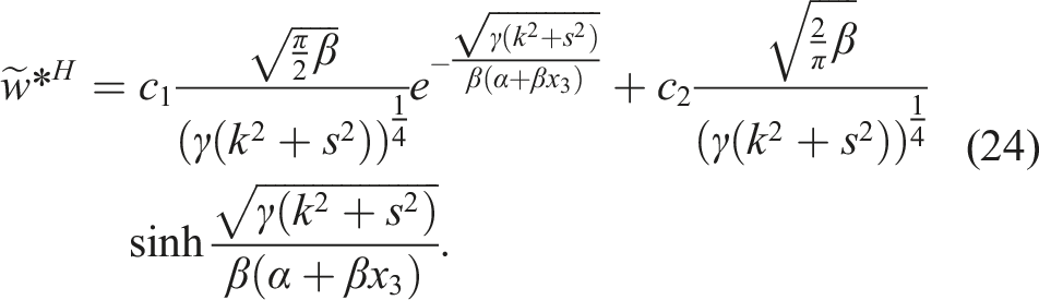
When ν = 1/2, the parabolic velocity profile solution described in (12) is obtained, as the solutions in (22), which involve the modified Bessel functions of first and second kind are reduces to simpler forms

{\tilde{w}}^{* H} = c_{1} \frac{\sqrt{\frac{π}{2} β}}{{(γ (k^{2} + s^{2}))}^{\frac{1}{4}}} e^{- \frac{\sqrt{γ (k^{2} + s^{2})}}{β (α + β x_{3})}} + c_{2} \frac{\sqrt{\frac{2}{π} β}}{{(γ (k^{2} + s^{2}))}^{\frac{1}{4}}} \sinh \frac{\sqrt{γ (k^{2} + s^{2})}}{β (α + β x_{3})} .

(24)

Considering again the general power function velocity profile, the Green’s function for the ordinary differential equation, valid for $- α / β < (x_{3}, x_{3}^{0}) < \infty$ and ν > 0, is expressed as

{\tilde{w}}^{*} (x_{3}) = \frac{2 F_{0} γ ν}{β \sqrt{μ (α + β x_{3})} {(α + β x_{3}^{0})}^{\frac{1}{ν} + \frac{1}{2}}} \{\begin{cases} I_{ν} (\frac{2 ν \sqrt{γ (k^{2} + s^{2})}}{β {(α + γ x_{3}^{0})}^{\frac{1}{2 ν}}}) K_{ν} (\frac{2 ν \sqrt{γ (k^{2} + s^{2})}}{β {(α + β x_{3})}^{\frac{1}{2 ν}}}) x_{3} < x_{3}^{0}, \\ I_{ν} (\frac{2 ν \sqrt{γ (k^{2} + s^{2})}}{β {(α + β x_{3})}^{\frac{1}{2 ν}}}) K_{ν} (\frac{2 ν \sqrt{γ (k^{2} + s^{2})}}{β {(α + β x_{3}^{0})}^{\frac{1}{2 ν}}}) x_{3} > x_{3}^{0} . \end{cases}

(25)

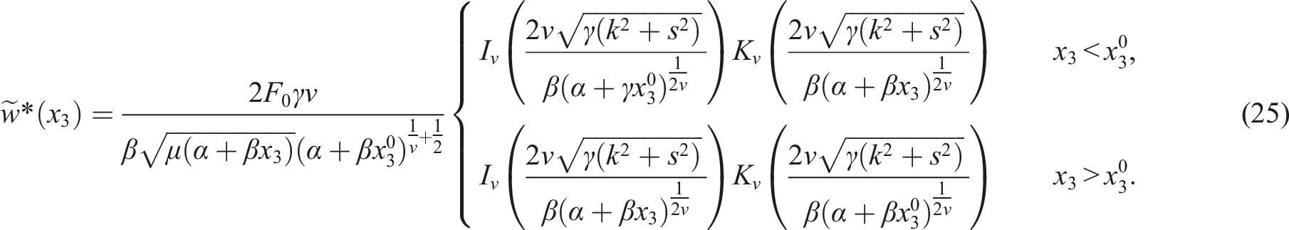
Using the formula provided by Oberhettinger (1958), the product of Bessel functions of non-integer order can be transformed into the form that is useful for the inversion of integral transforms.

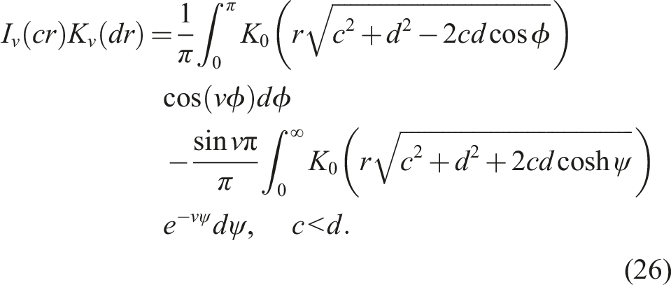
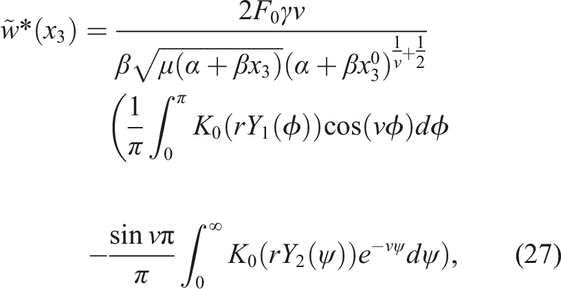
\begin{aligned} I_{ν} (c r) K_{ν} (d r) = & \frac{1}{π} \int_{0}^{π} K_{0} (r \sqrt{c^{2} + d^{2} - 2 c d \cos ϕ}) \cos (ν ϕ) d ϕ \\ - \frac{\sin ν π}{π} \int_{0}^{\infty} K_{0} (r \sqrt{c^{2} + d^{2} + 2 c d \cosh ψ}) e^{- ν ψ} d ψ, c < d . \end{aligned}

(26)

The above formula for integral transform inversion has been brought to attention by Watanabe and Payton (1997, 2004). Using (26) we obtain

{\tilde{w}}^{*} (x_{3}) = \frac{2 F_{0} γ ν}{β \sqrt{μ (α + β x_{3})} {(α + β x_{3}^{0})}^{\frac{1}{ν} + \frac{1}{2}}} (\frac{1}{π} \int_{0}^{π} K_{0} (r Y_{1} (ϕ)) \cos (ν ϕ) d ϕ - \frac{\sin ν π}{π} \int_{0}^{\infty} K_{0} (r Y_{2} (ψ)) e^{- ν ψ} d ψ),

(27)

where

r = \sqrt{k^{2} + s^{2}}

. Y₁ (ϕ) and Y₂ (ψ) are defined as

Y_{1} (ϕ) = \frac{2 ν}{β} \sqrt{\frac{γ}{{(α + β x_{3}^{0})}^{\frac{1}{ν}}} + \frac{γ}{{(α + β x_{3})}^{\frac{1}{ν}}} - \frac{2 γ \cos ϕ}{{(α + β x_{3}^{0})}^{\frac{1}{2 ν}} {(α + β x_{3})}^{\frac{1}{2 ν}}}},

(28)

Y_{2} (ψ) = \frac{2 ν}{β} \sqrt{\frac{γ}{{(α + β x_{3}^{0})}^{\frac{1}{ν}}} + \frac{γ}{{(α + β x_{3})}^{\frac{1}{ν}}} + \frac{2 γ \cosh ψ}{{(α + β x_{3}^{0})}^{\frac{1}{2 ν}} {(α + β x_{3})}^{\frac{1}{2 ν}}}} .

(29)

The inverse Laplace formula as per Oberhettinger and Badii (2012) for K_κ of order κ = 0 is

L^{- 1} (K_{0} (Y r)) = H (τ - Y) \frac{k^{\frac{1}{2}}}{{(τ^{2} - Y^{2})}^{\frac{1}{4}}} J_{- \frac{1}{2}} (k \sqrt{τ^{2} - Y^{2}}) \frac{π \sqrt{2}}{2 \sqrt{π}} .

(30)

The inverse Fourier transform formula obtained from Bateman et al. (1954) is written as

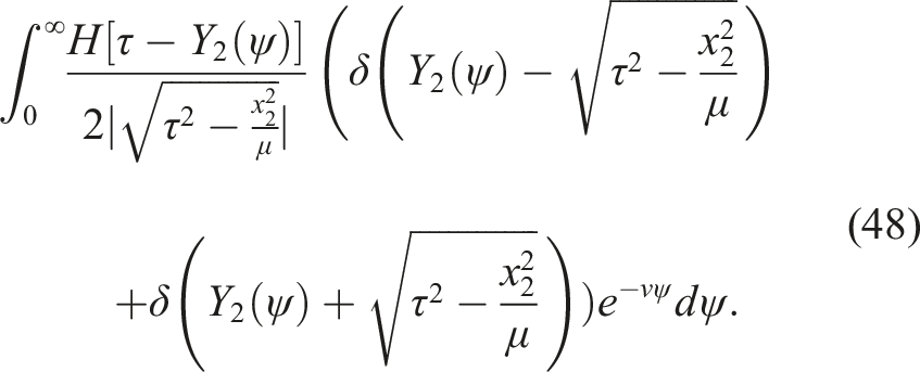
\begin{align} \frac{1}{2 π} \int_{- \infty}^{+ \infty} b^{- v - \frac{1}{2}} k^{- v - \frac{1}{2}} J_{n + ν + \frac{1}{2}} (b k) e^{- i k {\hat{x}}_{2}} b d k \\ = {(- i)}^{n} n! {(2 π)}^{(- \frac{1}{2})} 2^{- ν} {[1 - {(\frac{{\hat{x}}_{2}}{b})}^{2}]}^{ν} P_{n}^{ν, ν} (\frac{{\hat{x}}_{2}}{b}) Γ {(n + ν + 1)}^{- 1} H [1 - | \frac{{\hat{x}}_{2}}{b} |] for R e ν > - 1 . \end{align}

(31)

For n = 0 we obtain

\frac{1}{2 π} b^{\frac{1}{2}} \int_{- \infty}^{+ \infty} k^{- ν - \frac{1}{2}} J_{ν + \frac{1}{2}} (b k) e^{- i k \hat{x_{2}}} d k = \frac{1}{\sqrt{2 π}} {[\frac{b}{2} (1 - {(\frac{{\hat{x}}_{2}}{b})}^{2})]}^{ν} Γ {(ν + 1)}^{- 1} H [1 - |\frac{{\hat{x}}_{2}}{b}|] for R e ν > - 1 .

(32)

The integral provided in Bateman et al. (1954) only for values satisfying Reν > − 1. Therefore for our case we evaluate the limiting case as ν → −1. When this limit is taken, the quadratic in ${\hat{x}}_{2}$ , together with gamma and Heaviside functions reduces to a pair(sum) of Dirac delta generalized functions at ${\hat{x}}_{2} = b$ and ${\hat{x}}_{2} = - b$ . As limit ν → −1 (32) becomes following expression

F^{- 1} \{k^{\frac{1}{2}} J_{- \frac{1}{2}} (b k)\} = \frac{1}{\sqrt{2 π}} \{\frac{δ ({\hat{x}}_{2} - b)}{\sqrt{b}} + \frac{δ ({\hat{x}}_{2} + b)}{\sqrt{b}}\} b > 0 .

(33)

The initial form of the Green’s function is written as

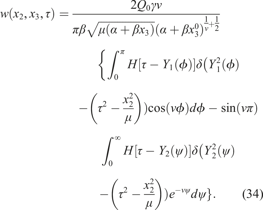
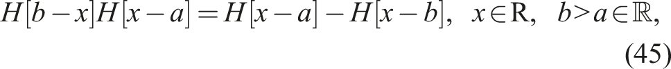
\begin{aligned} w (x_{2}, x_{3}, τ) = & \frac{2 Q_{0} γ ν}{π β \sqrt{μ (α + β x_{3})} {(α + β x_{3}^{0})}^{\frac{1}{ν} + \frac{1}{2}}} \{\int_{0}^{π} H [τ - Y_{1} (ϕ)] δ (Y_{1}^{2} (ϕ) - (τ^{2} - \frac{x_{2}^{2}}{μ})) \cos (ν ϕ) d ϕ \\ - \sin (ν π) \int_{0}^{\infty} H [τ - Y_{2} (ψ)] δ (Y_{2}^{2} (ψ) - (τ^{2} - \frac{x_{2}^{2}}{μ})) e^{- ν ψ} d ψ\} . \end{aligned}

(34)

The following identity have used in (34).

\frac{1}{| b |} [δ (x - b) + δ (x + b)] = 2 δ (x^{2} - b^{2}) .

(35)

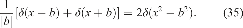
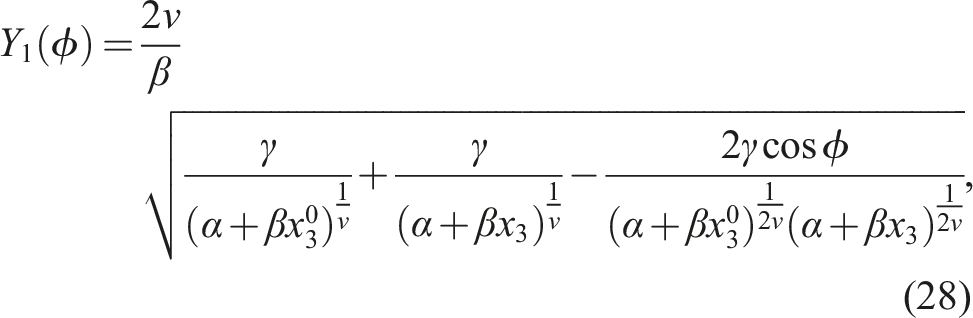
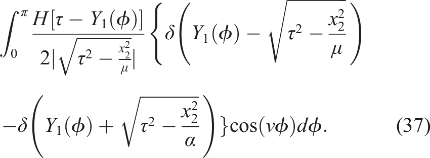
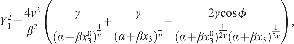
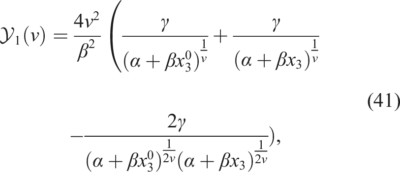
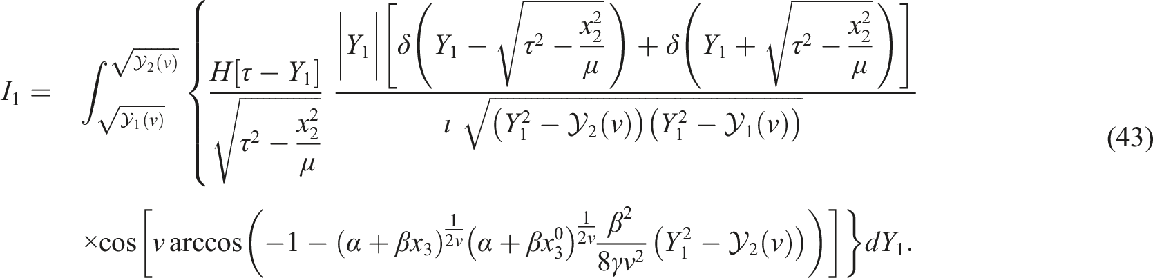
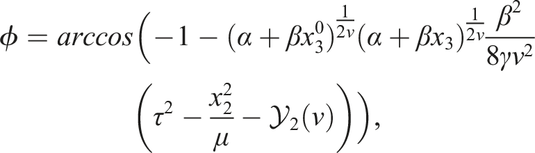
Now let’s use the identity (35), but in reverse, to examine the first integral in (34) using Y₁ (ϕ) as variable term. that is,

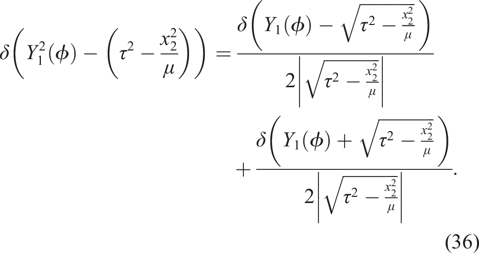
δ (Y_{1}^{2} (ϕ) - (τ^{2} - \frac{x_{2}^{2}}{μ})) = \frac{δ (Y_{1} (ϕ) - \sqrt{τ^{2} - \frac{x_{2}^{2}}{μ}})}{2 | \sqrt{τ^{2} - \frac{x_{2}^{2}}{μ}} |} + \frac{δ (Y_{1} (ϕ) + \sqrt{τ^{2} - \frac{x_{2}^{2}}{μ}})}{2 | \sqrt{τ^{2} - \frac{x_{2}^{2}}{μ}} |} .

(36)

The first integral is rewritten as

\int_{0}^{π} \frac{H [τ - Y_{1} (ϕ)]}{2 | \sqrt{τ^{2} - \frac{x_{2}^{2}}{μ}} |} \{δ (Y_{1} (ϕ) - \sqrt{τ^{2} - \frac{x_{2}^{2}}{μ}}) - δ (Y_{1} (ϕ) + \sqrt{τ^{2} - \frac{x_{2}^{2}}{α}})\} \cos (ν ϕ) d ϕ .

(37)

Now, the integration variable changed as Y₁ ≡ Y₁ (ϕ) so we obtain the relations

Y_{1}^{2} = \frac{4 ν^{2}}{β^{2}} (\frac{γ}{{(α + β x_{3}^{0})}^{\frac{1}{ν}}} + \frac{γ}{{(α + β x_{3})}^{\frac{1}{ν}}} - \frac{2 γ \cos ϕ}{{(α + β x_{3}^{0})}^{\frac{1}{2 ν}} {(α + β x_{3})}^{\frac{1}{2 ν}}}),

d ϕ = \frac{{(α + β x_{3}^{0})}^{\frac{1}{2 ν}} {(α + β x_{3})}^{\frac{1}{2 ν}} | Y_{1} | β^{2}}{4 γ ν^{2} \sin ϕ} d Y_{1} .

(38)

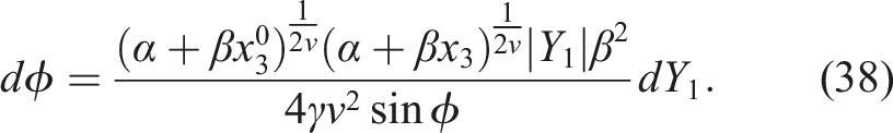
By simple rearrangement, the value of cos ϕ is obtained from (38-a) and sin ϕ is derived using the formula $\sin ϕ = \sqrt{(1 - \cos ϕ) (1 + c o s ϕ)}$

\cos ϕ = \frac{{(α + β x_{3})}^{\frac{1}{2 ν}} {(α + β x_{3}^{0})}^{\frac{1}{2 ν}}}{2 γ} (\frac{γ}{{(α + β x_{3}^{0})}^{\frac{1}{ν}}} + \frac{γ}{{(α + β x_{3})}^{\frac{1}{ν}}} - \frac{β^{2} Y_{1}^{2}}{4 ν^{2}}),

1 + \cos ϕ = - \frac{{(α + β x_{3})}^{\frac{1}{2 ν}} {(α + β x_{3}^{0})}^{\frac{1}{2 ν}}}{2 γ} \{\frac{β^{2}}{4 ν^{2}} [Y_{1}^{2} - Y_{2} (ν)]\},

(39)

1 - \cos ϕ = \frac{{(α + β x_{3})}^{\frac{1}{2 ν}} {(α + β x_{3}^{0})}^{\frac{1}{2 ν}}}{2 γ} \{\frac{β^{2}}{4 ν^{2}} [Y_{1}^{2} - Y_{1} (ν)]\},

(40)

where

Y_{1} (ν)

and

Y_{2} (ν)

are defined as

Y_{1} (ν) = \frac{4 ν^{2}}{β^{2}} (\frac{γ}{{(α + β x_{3}^{0})}^{\frac{1}{ν}}} + \frac{γ}{{(α + β x_{3})}^{\frac{1}{ν}}} - \frac{2 γ}{{(α + β x_{3}^{0})}^{\frac{1}{2 ν}} {(α + β x_{3})}^{\frac{1}{2 ν}}}),

(41)

Y_{2} (ν) = \frac{4 ν^{2}}{β^{2}} (\frac{γ}{{(α + β x_{3}^{0})}^{\frac{1}{ν}}} + \frac{γ}{{(α + β x_{3})}^{\frac{1}{ν}}} + \frac{2 γ}{{(α + β x_{3}^{0})}^{\frac{1}{2 ν}} {(α + β x_{3})}^{\frac{1}{2 ν}}}) .

(42)

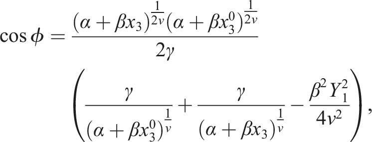
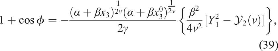
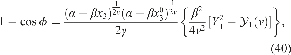
The first integral can be rewritten using (38)–(40) as follows

\begin{aligned} I_{1} = & \int_{\sqrt{Y_{1} (ν)}}^{\sqrt{Y_{2} (ν)}} \{\frac{H [τ - Y_{1}]}{\sqrt{τ^{2} - \frac{x_{2}^{2}}{μ}}} \frac{| Y_{1} | [δ (Y_{1} - \sqrt{τ^{2} - \frac{x_{2}^{2}}{μ}}) + δ (Y_{1} + \sqrt{τ^{2} - \frac{x_{2}^{2}}{μ}})]}{ι \sqrt{(Y_{1}^{2} - Y_{2} (ν)) (Y_{1}^{2} - Y_{1} (ν))}} \\ \times \cos [ν \arccos (- 1 - {(α + β x_{3})}^{\frac{1}{2 ν}} {(α + β x_{3}^{0})}^{\frac{1}{2 ν}} \frac{β^{2}}{8 γ ν^{2}} (Y_{1}^{2} - Y_{2} (ν)))]\} d Y_{1} . \end{aligned}

(43)

Restricting $τ^{2} - x_{2}^{2} / μ \geq 0$ the equation (43) becomes

\begin{aligned} I_{1} = & - i \{\frac{H [\sqrt{τ^{2} - \frac{x_{2}^{2}}{μ}} - \sqrt{Y_{1} (ν)}] H [\sqrt{Y_{2} (ν)} - \sqrt{τ^{2} - \frac{x_{2}^{2}}{μ}}]}{\sqrt{(τ^{2} - \frac{x_{2}^{2}}{μ} - Y_{2} (ν)) (τ^{2} - \frac{x_{2}^{2}}{μ} - Y_{1} (ν))}} \\ + \frac{H [\sqrt{Y_{2} (ν)} + \sqrt{τ^{2} - \frac{x_{2}^{2}}{μ}}] H [- \sqrt{τ^{2} - \frac{x_{2}^{2}}{μ}} - \sqrt{Y_{1} (ν)}]}{\sqrt{(τ^{2} - \frac{x_{2}^{2}}{μ} - Y_{2} (ν)) (τ^{2} - \frac{x_{2}^{2}}{μ} - Y_{1} (ν))}}\} \\ \times \cos [ν \arccos (- 1 - {(α + β x_{3}^{0})}^{\frac{1}{2 ν}} {(α + β x_{3})}^{\frac{1}{2 ν}} \frac{β^{2}}{8 γ ν^{2}} (τ^{2} - \frac{x_{2}^{2}}{μ} - Y_{2} (ν)))] . \end{aligned}

(44)

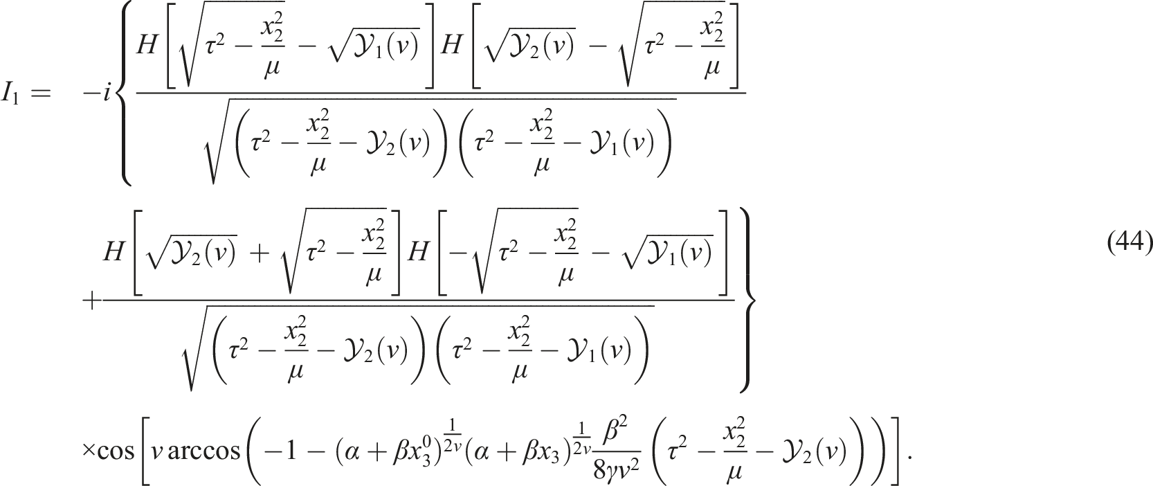
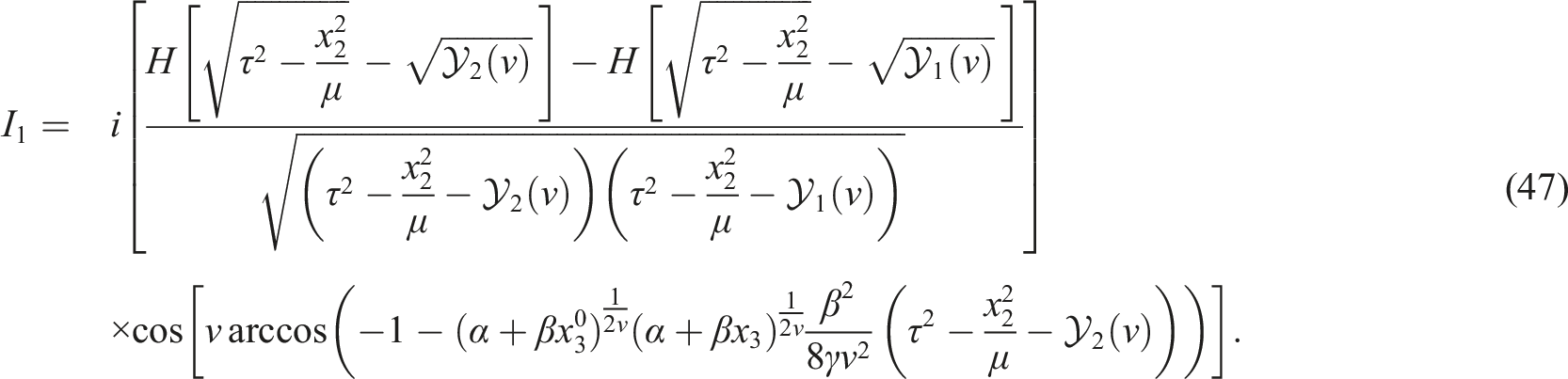
By applying the following Heaviside step function identities,

H [b - x] H [x - a] = H [x - a] - H [x - b], x \in R, b > a \in R,

(45)

H [b] H [- a] = 0, a, b > 0,

(46)

the integral I₁ simplifies to

\begin{aligned} I_{1} = & i [\frac{H [\sqrt{τ^{2} - \frac{x_{2}^{2}}{μ}} - \sqrt{Y_{2} (ν)}] - H [\sqrt{τ^{2} - \frac{x_{2}^{2}}{μ}} - \sqrt{Y_{1} (ν)}]}{\sqrt{(τ^{2} - \frac{x_{2}^{2}}{μ} - Y_{2} (ν)) (τ^{2} - \frac{x_{2}^{2}}{μ} - Y_{1} (ν))}}] \\ \times \cos [ν \arccos (- 1 - {(α + β x_{3}^{0})}^{\frac{1}{2 ν}} {(α + β x_{3})}^{\frac{1}{2 ν}} \frac{β^{2}}{8 γ ν^{2}} (τ^{2} - \frac{x_{2}^{2}}{μ} - Y_{2} (ν)))] . \end{aligned}

(47)

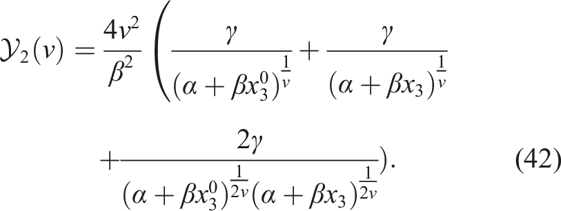
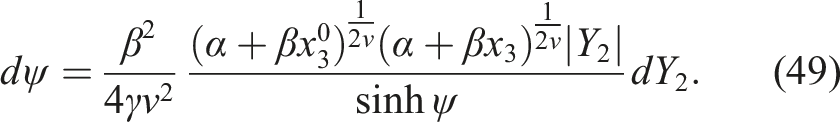
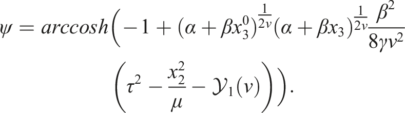
Now, concentrate on the second integral of (34)

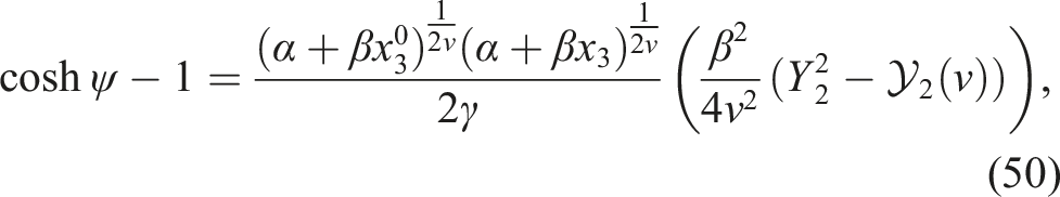
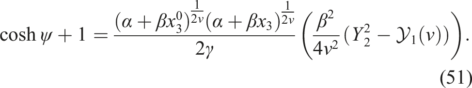
\int_{0}^{\infty} \frac{H [τ - Y_{2} (ψ)]}{2 | \sqrt{τ^{2} - \frac{x_{2}^{2}}{μ}} |} (δ (Y_{2} (ψ) - \sqrt{τ^{2} - \frac{x_{2}^{2}}{μ}}) + δ (Y_{2} (ψ) + \sqrt{τ^{2} - \frac{x_{2}^{2}}{μ}})) e^{- ν ψ} d ψ .

(48)

Now, the integration variable changed to Y₂ ≡ Y₁ (ψ) so we obtain the relations

d ψ = \frac{β^{2}}{4 γ ν^{2}} \frac{{(α + β x_{3}^{0})}^{\frac{1}{2 ν}} {(α + β x_{3})}^{\frac{1}{2 ν}} | Y_{2} |}{\sinh ψ} d Y_{2} .

(49)

To derive the value of sinh ψ the following formula is used $\sinh ψ = \sqrt{(\cosh ψ - 1) (\cosh ψ + 1)}$ and

\cosh ψ - 1 = \frac{{(α + β x_{3}^{0})}^{\frac{1}{2 ν}} {(α + β x_{3})}^{\frac{1}{2 ν}}}{2 γ} (\frac{β^{2}}{4 ν^{2}} (Y_{2}^{2} - Y_{2} (ν))),

(50)

\cosh ψ + 1 = \frac{{(α + β x_{3}^{0})}^{\frac{1}{2 ν}} {(α + β x_{3})}^{\frac{1}{2 ν}}}{2 γ} (\frac{β^{2}}{4 ν^{2}} (Y_{2}^{2} - Y_{1} (ν))) .

(51)

Since the upper limit in (48) goes to infinity, the integration is a bit simpler, which simplifies the final expression using the Heaviside function. For I₂, we obtain the following

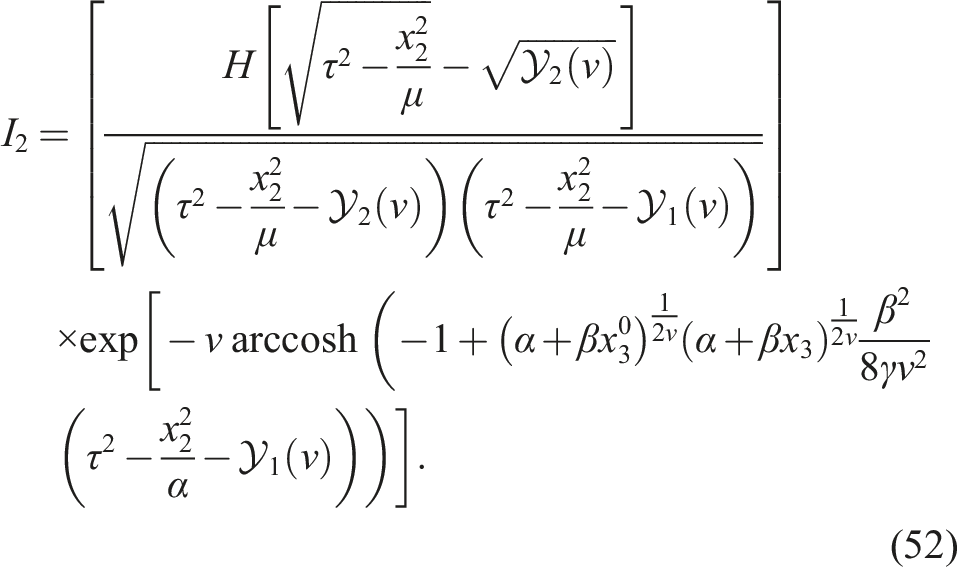
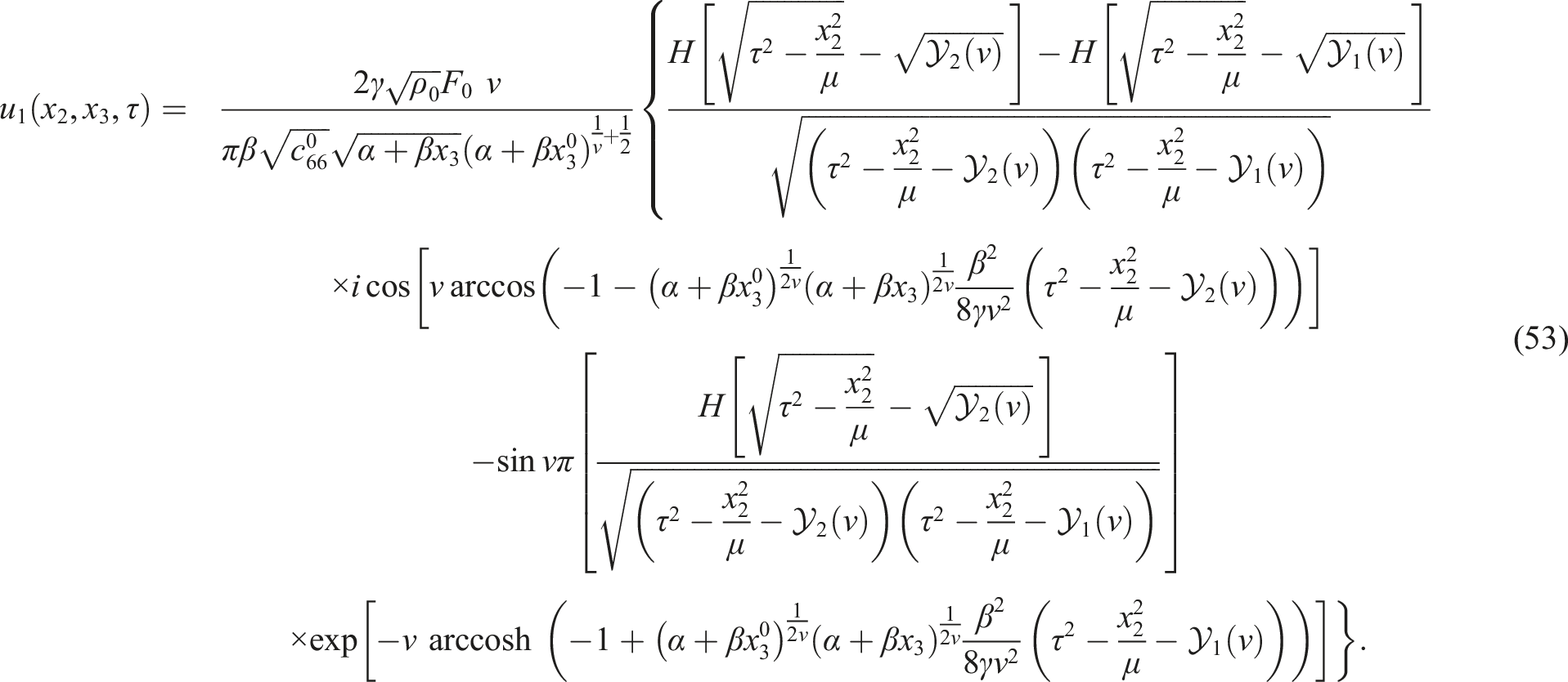
\begin{matrix} I_{2} = & [\frac{H [\sqrt{τ^{2} - \frac{x_{2}^{2}}{μ}} - \sqrt{Y_{2} (ν)}]}{\sqrt{(τ^{2} - \frac{x_{2}^{2}}{μ} - Y_{2} (ν)) (τ^{2} - \frac{x_{2}^{2}}{μ} - Y_{1} (ν))}}] \\ \times \exp [- ν arccosh (- 1 + {(α + β x_{3}^{0})}^{\frac{1}{2 ν}} {(α + β x_{3})}^{\frac{1}{2 ν}} \frac{β^{2}}{8 γ ν^{2}} (τ^{2} - \frac{x_{2}^{2}}{α} - Y_{1} (ν)))] . \end{matrix}

(52)

By substituting (42) and (52) in (34) the Green’s function is finally simplified to the following form

\begin{aligned} u_{1} (x_{2}, x_{3}, τ) = & \frac{2 γ \sqrt{ρ_{0}} F_{0} ν}{π β \sqrt{c_{66}^{0}} \sqrt{α + β x_{3}} {(α + β x_{3}^{0})}^{\frac{1}{ν} + \frac{1}{2}}} \{\frac{H [\sqrt{τ^{2} - \frac{x_{2}^{2}}{μ}} - \sqrt{Y_{2} (ν)}] - H [\sqrt{τ^{2} - \frac{x_{2}^{2}}{μ}} - \sqrt{Y_{1} (ν)}]}{\sqrt{(τ^{2} - \frac{x_{2}^{2}}{μ} - Y_{2} (ν)) (τ^{2} - \frac{x_{2}^{2}}{μ} - Y_{1} (ν))}} \\ \times i \cos [ν \arccos (- 1 - {(α + β x_{3}^{0})}^{\frac{1}{2 ν}} {(α + β x_{3})}^{\frac{1}{2 ν}} \frac{β^{2}}{8 γ ν^{2}} (τ^{2} - \frac{x_{2}^{2}}{μ} - Y_{2} (ν)))] \\ - \sin ν π [\frac{H [\sqrt{τ^{2} - \frac{x_{2}^{2}}{μ}} - \sqrt{Y_{2} (ν)}]}{\sqrt{(τ^{2} - \frac{x_{2}^{2}}{μ} - Y_{2} (ν)) (τ^{2} - \frac{x_{2}^{2}}{μ} - Y_{1} (ν))}}] \\ \times \exp [- ν arccosh (- 1 + {(α + β x_{3}^{0})}^{\frac{1}{2 ν}} {(α + β x_{3})}^{\frac{1}{2 ν}} \frac{β^{2}}{8 γ ν^{2}} (τ^{2} - \frac{x_{2}^{2}}{μ} - Y_{1} (ν)))]\} . \end{aligned}

(53)

4.1. The parabolic velocity profile

The parabolic velocity profile, that is, ν = 1/2, acts as a benchmark test for the equation given in (53). If we consider the following identities, we confirm the uniqueness of the Green’s function as expected

c o s (\frac{1}{2} ϕ) = \sqrt{\frac{1 + c o s (ϕ)}{2}}, for 0 < ϕ < π,

(54)

\exp (- \frac{1}{2} ψ) = \sqrt{\frac{c o s h (ψ) + 1}{2}} - \sqrt{\frac{c o s h (ψ) - 1}{2}} .

(55)

From equation (53) ϕ and ψ will be

ϕ = a r c c o s (- 1 - {(α + β x_{3}^{0})}^{\frac{1}{2 ν}} {(α + β x_{3})}^{\frac{1}{2 ν}} \frac{β^{2}}{8 γ ν^{2}} (τ^{2} - \frac{x_{2}^{2}}{μ} - Y_{2} (ν))),

ψ = a r c c o s h (- 1 + {(α + β x_{3}^{0})}^{\frac{1}{2 ν}} {(α + β x_{3})}^{\frac{1}{2 ν}} \frac{β^{2}}{8 γ ν^{2}} (τ^{2} - \frac{x_{2}^{2}}{μ} - Y_{1} (ν))) .

From (54) and (55)

c o s (\frac{1}{2} ϕ) = \sqrt{- (α + β x_{3}^{0}) (α + β x_{3}) \frac{β^{2}}{4 γ} (τ^{2} - \frac{x_{2}^{2}}{μ} - Y_{2} (\frac{1}{2}))},

c o s h (ψ) = - 1 + (α + β x_{3}^{0}) (α + β x_{3}) \frac{β^{2}}{4 γ} (τ^{2} - \frac{x_{2}^{2}}{μ} - Y_{1} (\frac{1}{2})) .

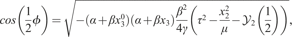
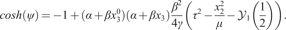
We get the simplified form of the parabolic velocity profile after some algebraic work as

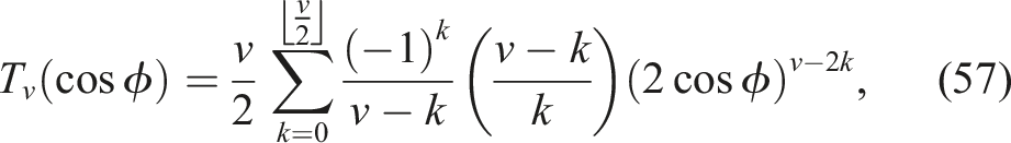
\begin{aligned} u_{1} (x_{2}, x_{3}, τ) = & \frac{F_{0} \sqrt{γ} \sqrt{ρ_{0}}}{2 π \sqrt{c_{66}^{0}} {(α + β x_{3}^{0})}^{2}} \{\frac{H [\sqrt{τ^{2} - \frac{x_{2}^{2}}{μ}} - \frac{1}{β} \sqrt{\frac{γ}{{(α + β x_{3}^{0})}^{2}} + \frac{γ}{{(α + β x_{3})}^{2}} - \frac{2 γ}{(α + β x_{3}^{0}) (α + β x_{3})}}]}{\sqrt{τ^{2} - \frac{x_{2}^{2}}{μ} - \frac{1}{β^{2}} (\frac{γ}{{(α + β x_{3}^{0})}^{2}} + \frac{γ}{{(α + β x_{3})}^{2}} - \frac{2 γ}{(α + β x_{3}^{0}) (α + β x_{3})})}} \\ - \frac{H [\sqrt{τ^{2} - \frac{x_{2}^{2}}{μ}} - \frac{1}{β} \sqrt{\frac{γ}{{(α + β x_{3}^{0})}^{2}} + \frac{γ}{{(α + β x_{3})}^{2}} + \frac{2 γ}{(α + β x_{3}^{0}) (α + β x_{3})}}]}{\sqrt{τ^{2} - \frac{x_{2}^{2}}{μ} - \frac{1}{β^{2}} (\frac{γ}{{(α + β x_{3}^{0})}^{2}} + \frac{γ}{{(α + β x_{3})}^{2}} + \frac{2 γ}{(α + β x_{3}^{0}) (α + β x_{3})})}}\} . \end{aligned}

(56)

4.2. An expression for integer ν

It is possible to further simplify the complex Green’s function argument in (53) for integer values of ν. Then we can use a formula that involves Chebyshev polynomials and the cosine function cos (νϕ) = T_ν (cos ϕ),

T_{ν} (\cos ϕ) = \frac{ν}{2} \sum_{k = 0}^{⌊ \frac{ν}{2} ⌋} \frac{{(- 1)}^{k}}{ν - k} (\binom{ν - k}{k}) {(2 \cos ϕ)}^{ν - 2 k},

(57)

where ⌊.⌋ is the floor function. For

ν \in N

, (53) is expressed as

\begin{aligned} u_{1} (x_{2}, x_{3}, τ) = & \frac{2 γ \sqrt{ρ_{0}} F_{0} ν}{π β \sqrt{c_{66}^{0}} \sqrt{α + β x_{3}} {(α + β x_{3}^{0})}^{\frac{1}{ν} + \frac{1}{2}}} \{\frac{H [\sqrt{τ^{2} - \frac{x_{2}^{2}}{μ}} - \sqrt{Y_{2} (ν)}] - H [\sqrt{τ^{2} - \frac{x_{2}^{2}}{μ}} - \sqrt{Y_{1} (ν)}]}{\sqrt{[τ^{2} - \frac{x_{2}^{2}}{μ} - Y_{2} (ν)] [τ^{2} - \frac{x_{2}^{2}}{μ} - Y_{1} (ν)]}} \\ \times i T_{ν} [- 1 - \frac{{(α + β x_{3}^{0})}^{\frac{1}{2 ν}} {(α + β x_{3})}^{\frac{1}{2 ν}} β^{2}}{8 γ ν^{2}} (τ^{2} - \frac{x_{2}^{2}}{μ} - Y_{2} (ν))]\} . \end{aligned}

(58)

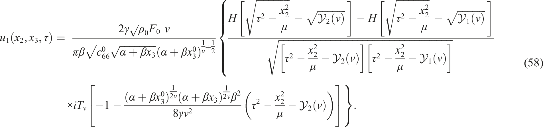
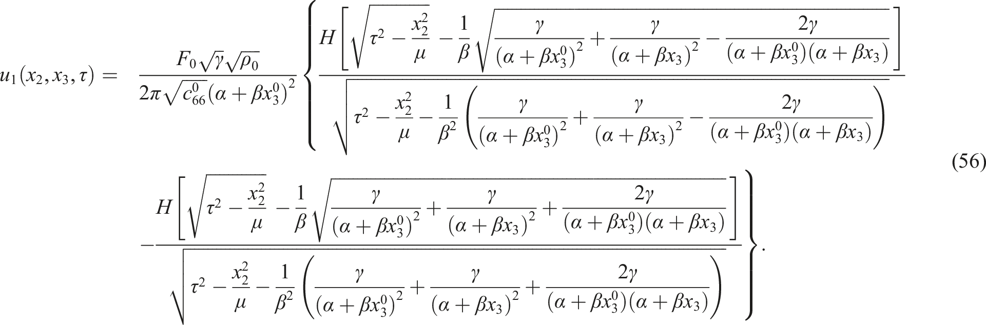
Equation (58) gives the required displacement in the transversely isotropic solid for the parabolic velocity profile. Note that when α → 1 and γ → 1, the displacement u₁ as obtained in (58) reduces to the expression as obtained by Daros (2013).

5. Wavefront

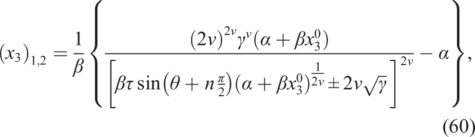
The two wavefronts are obtained from (53) as follows

W_{1,2} : τ = \sqrt{\frac{x_{2}^{2}}{μ} + Y_{1,2} (ν)} .

(59)

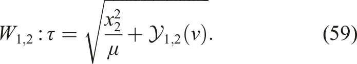
Their parametric expressions in cartesian coordinate system (x₂, x₃) are written as

{(x_{3})}_{1,2} = \frac{1}{β} \{\frac{{(2 ν)}^{2 ν} γ^{ν} (α + β x_{3}^{0})}{{[β τ \sin (θ + n \frac{π}{2}) {(α + β x_{3}^{0})}^{\frac{1}{2 ν}} \pm 2 ν \sqrt{γ}]}^{2 ν}} - α\},

(60)

{(x_{2})}_{1,2} = τ \sqrt{μ} \cos (θ + n \frac{π}{2}),

(61)

with n = 0 for

\sqrt{μ} > β / 2 ν

and n = 1 for

\sqrt{μ} < b / 2 ν

. The distinction in the parameter n arises from the presence of the ellipse’s major and minor axes, which are explicitly employed in the formulation of the parametric equations. The symbols ± correspond to the two wavefronts W₁ and W₂. In the parametric representation of the curves, θ ∈ [0, 2π] denotes the angular parameter.

We now briefly analyze the wavefronts. The vertical x₃-axis is taken as the major axis of the ellipse used in constructing the parametric equations, under the assumption that $\sqrt{μ} < β / (2 ν)$ . The reference angle θ increases counterclockwise, starting from the negative x₃-axis at θ = 0. A singularity occurs in ${(x_{3})}_{1}$ at θ = π, corresponding to the critical time

τ_{s} = \frac{2 ν \sqrt{γ}}{β {(α + β x_{3}^{0})}^{\frac{1}{2 ν}}} .

(62)

Then the W₁ wavefront reaches infinity. A secondary wave W₂ emerges after this event and diffracts from infinity. Watanabe and Payton (2004) had already discovered this secondary diffracted wave in radially inhomogeneous media.

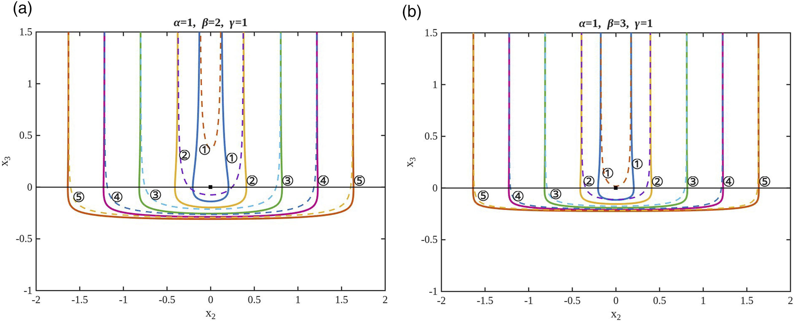
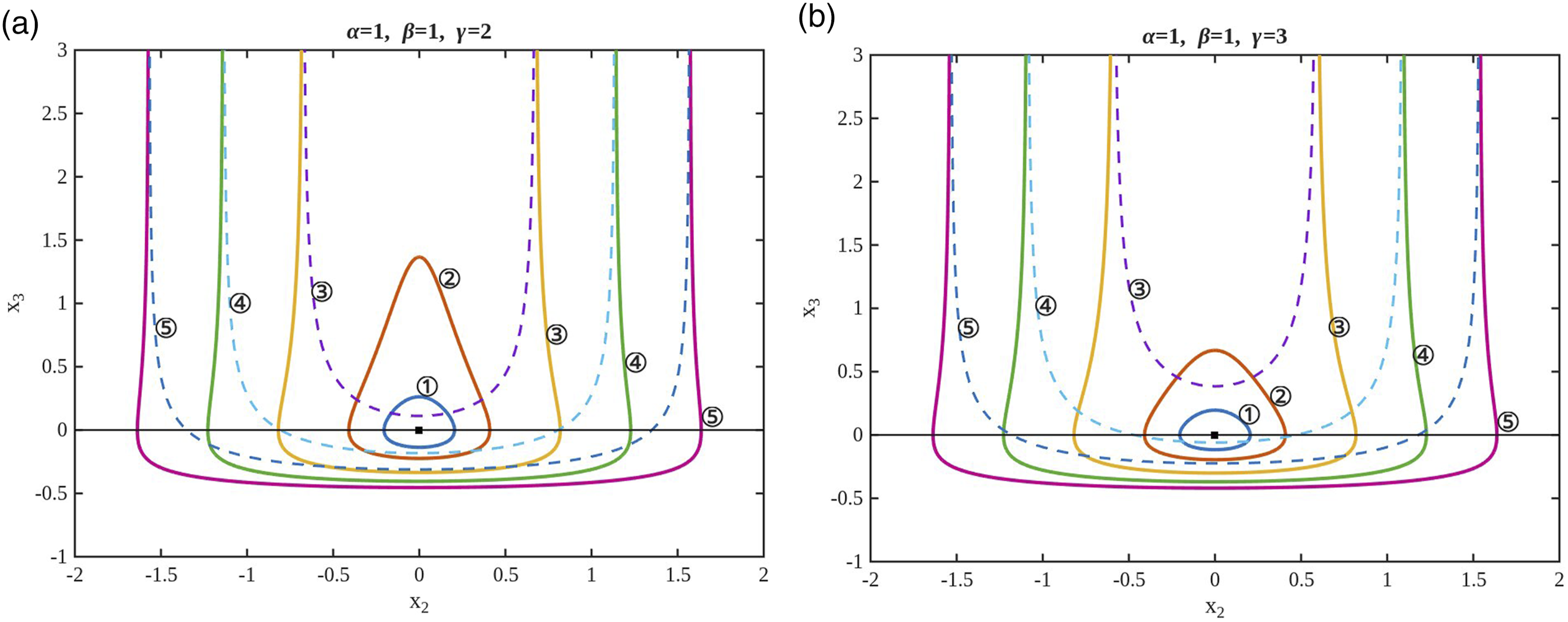
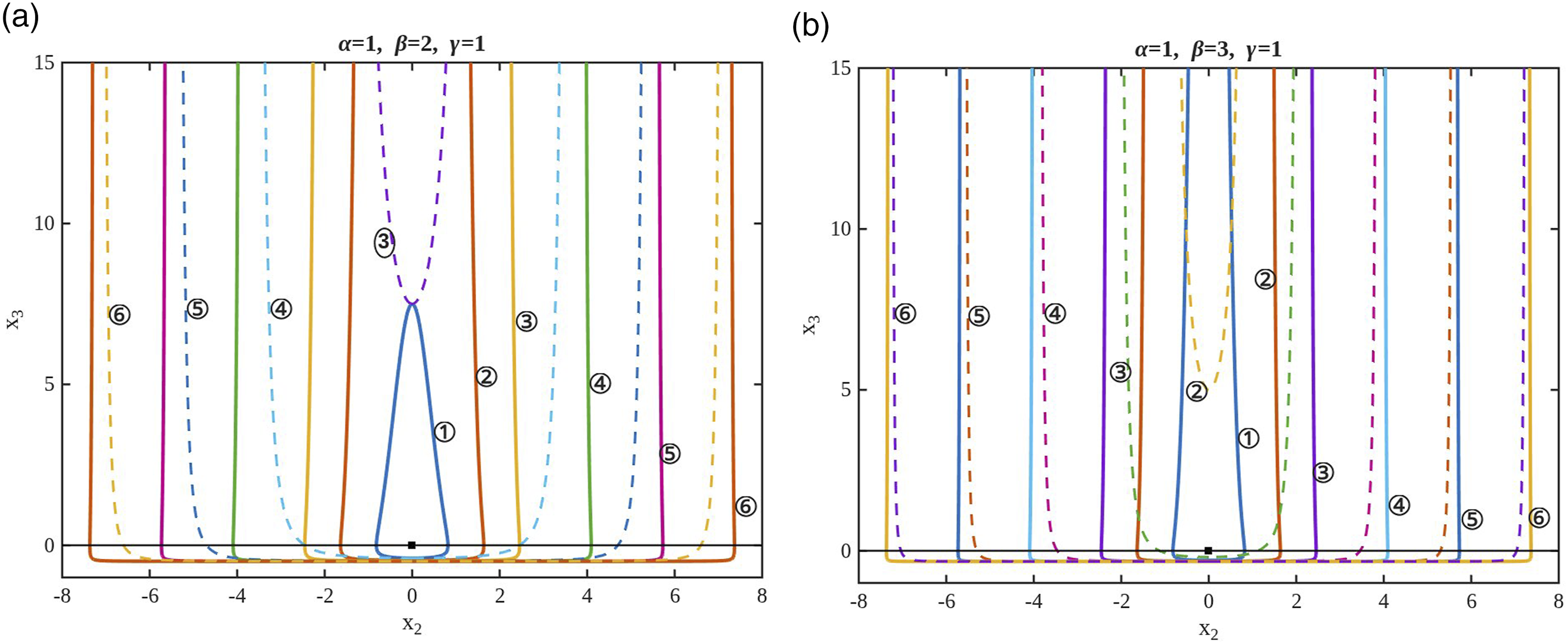
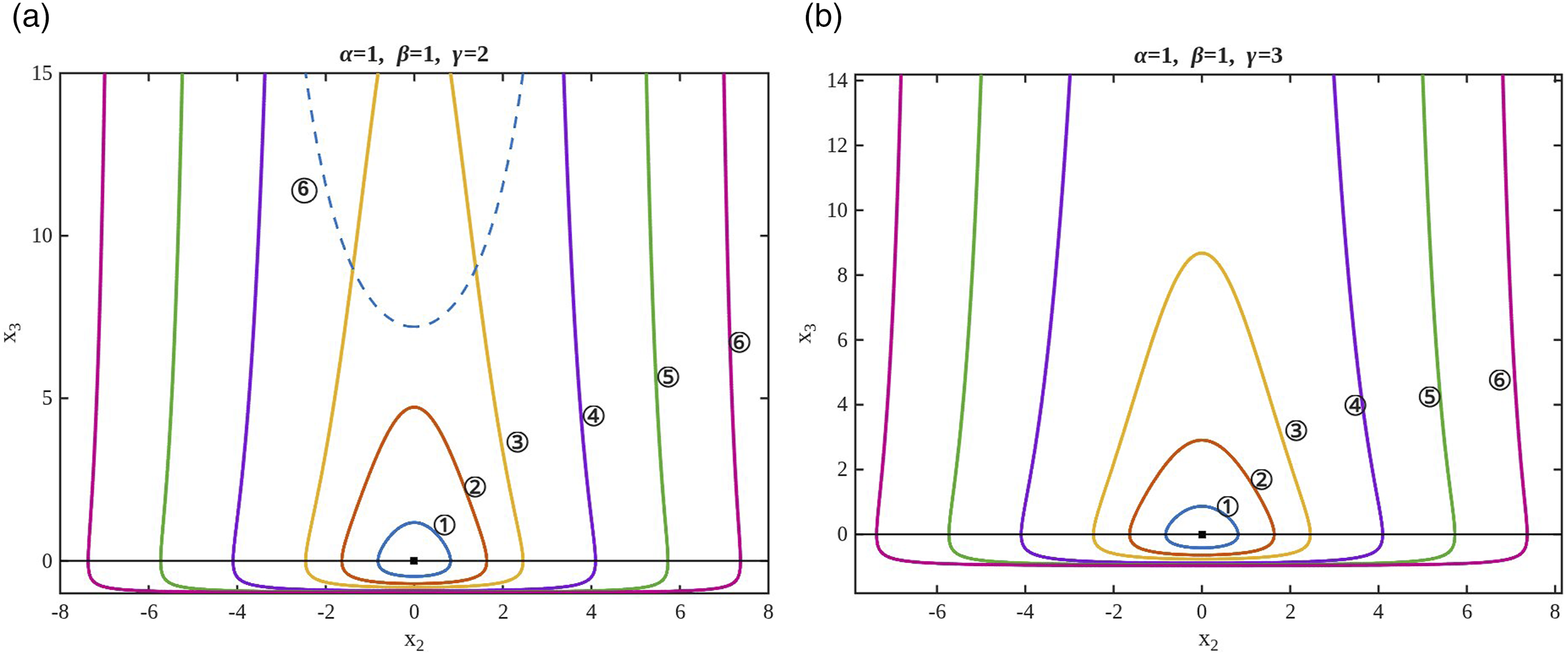
Figures 1 –8 illustrate the time evolution of the first (W₁) and second (W₂) SH-wavefronts generated by a point source located at (x₂ = 0, x₃ = 0) in a functionally graded transversely isotropic medium. The wavefronts are plotted as parametric curves in the (x₂, x₃)-plane for increasing nondimensional times τ, highlighting the role of the power law velocity profile and the inhomogeneity parameters α, β, and γ.

Figure 1.

Time evolution of the wavefronts for ν = 1/5, α = 1, β = 1, γ = 1 shown at τ = 0.25, 0.5, 1.0, 1.5, and 2.0, corresponding to curves 1–5, respectively.

Figure 2.

Time evolution of the wavefronts for ν = 1/5, β = 1, γ = 1, shown at τ = 0.25, 0.5, 1.0, 1.5, and 2.0, corresponding to curves 1–5, respectively when (a) α = 2, and (b) α = 3.

Figure 3.

Time evolution of the wavefronts for ν = 1/5, α = 1, γ = 1, shown at τ = 0.25, 0.5, 1.0, 1.5, and 2.0, corresponding to curves 1–5, respectively when (a) β = 2, and (b) β = 3.

Figure 4.

Time evolution of the wavefronts for ν = 1/5, α = 1, β = 1, shown at τ = 0.25, 0.5, 1.0, 1.5, and 2.0, corresponding to curves 1–5, respectively when (a) γ = 2, and (b) γ = 3.

Figure 5.

Time evolution of the wavefronts for ν = 2, α = 1, β = 1, γ = 1 shown at τ = 0.25, 0.5, 1.0, 1.5, and 2.0, corresponding to curves 1–5, respectively.

Figure 6.

Time evolution of the wavefronts for ν = 2, β = 1, γ = 1, shown at τ = 0.25, 0.5, 1.0, 1.5, and 2.0, corresponding to curves 1–5, respectively when (a) α = 2, and (b) α = 3.

Figure 7.

Time evolution of the wavefronts for ν = 1/5, α = 1, γ = 1, shown at τ = 0.25, 0.5, 1.0, 1.5, and 2.0, corresponding to curves 1–5, respectively when (a) β = 2, and (b) β = 3.

Figure 8.

Time evolution of the wavefronts for ν = 1/5, α = 1, β = 1, shown at τ = 0.25, 0.5, 1.0, 1.5, and 2.0, corresponding to curves 1–5, respectively when (a) γ = 2, and (b) γ = 3.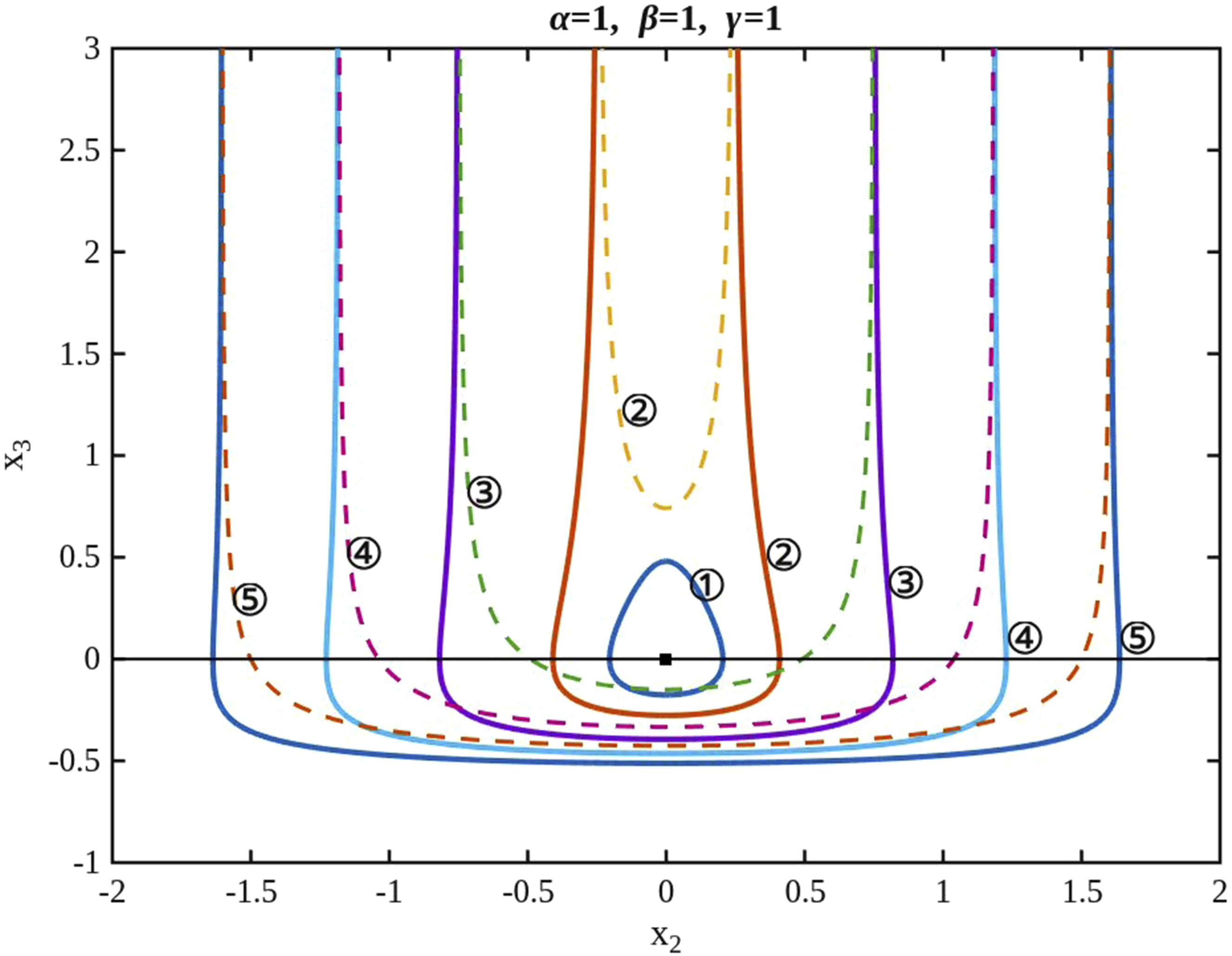

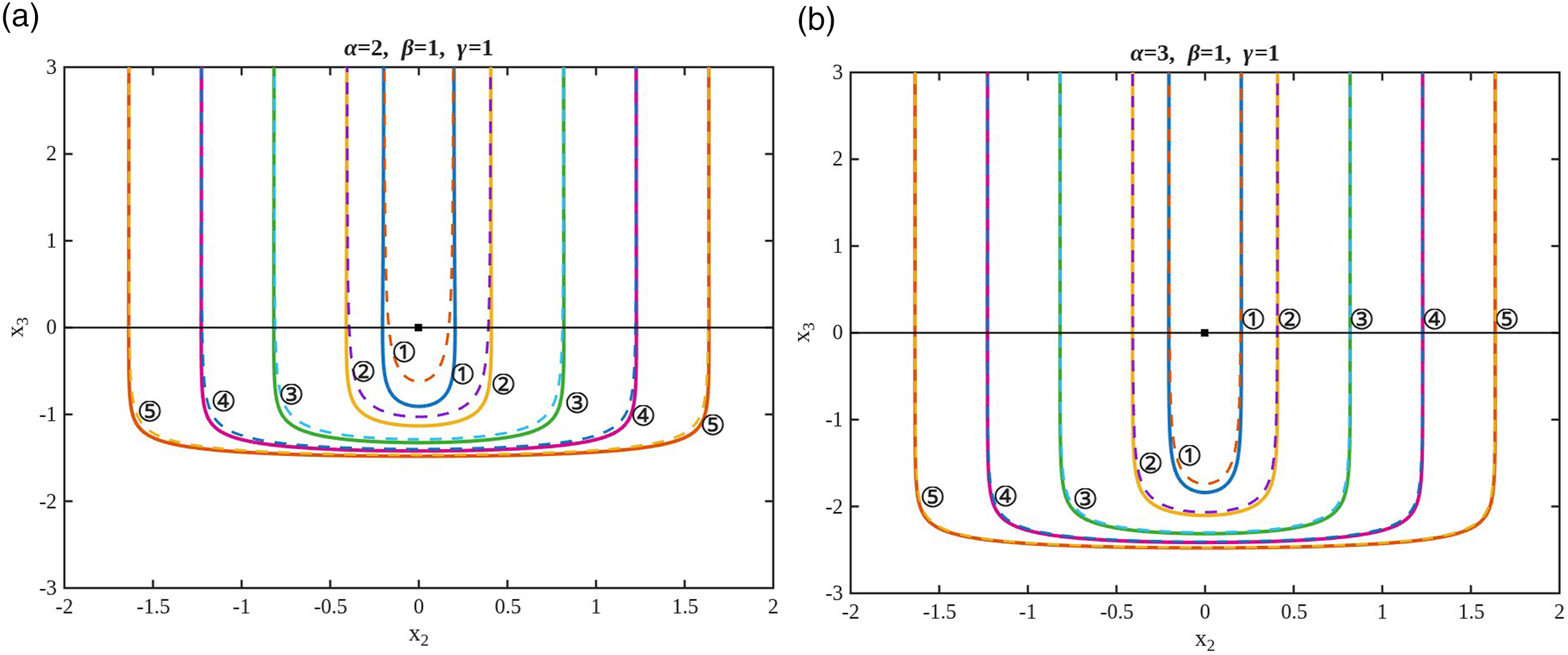
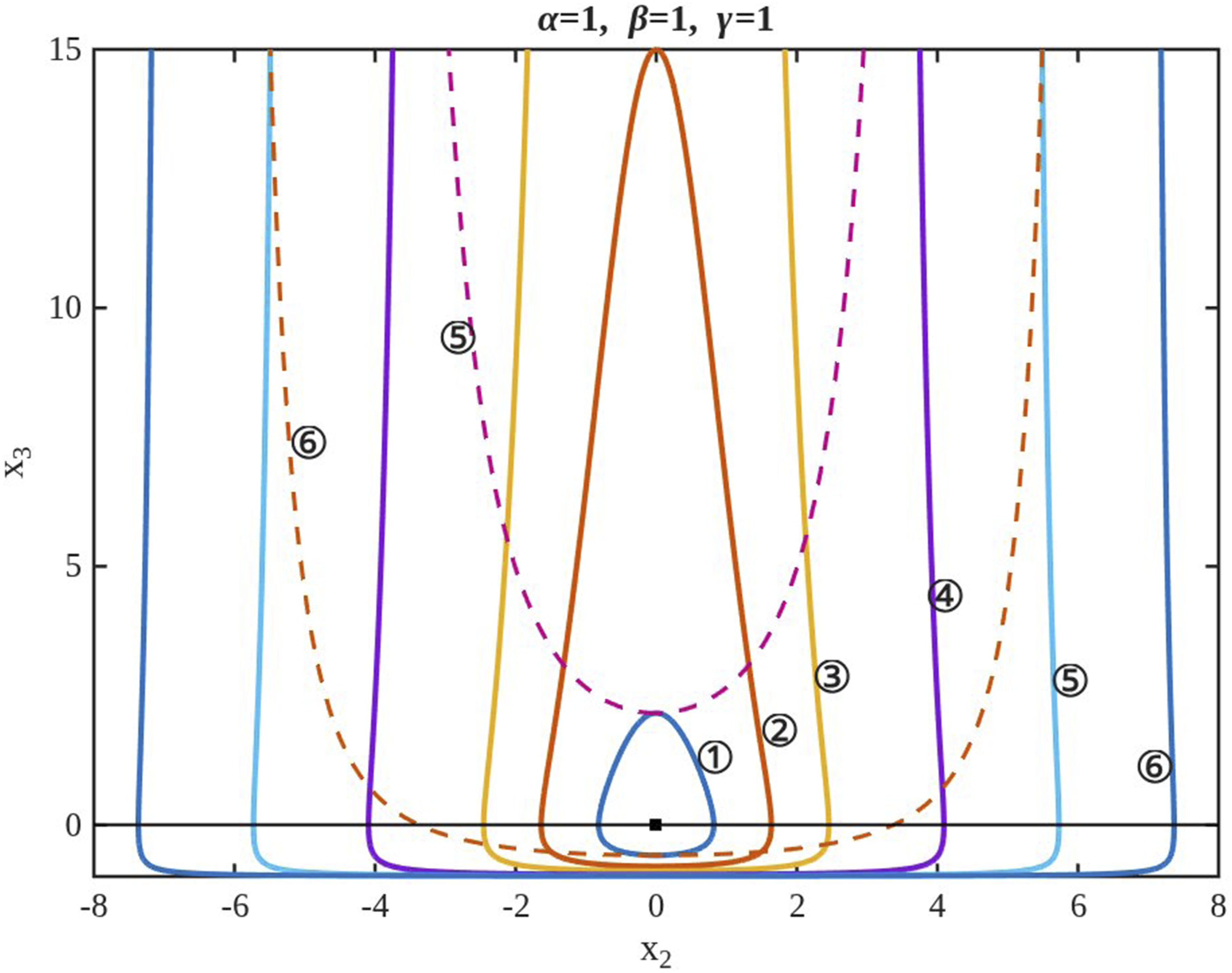
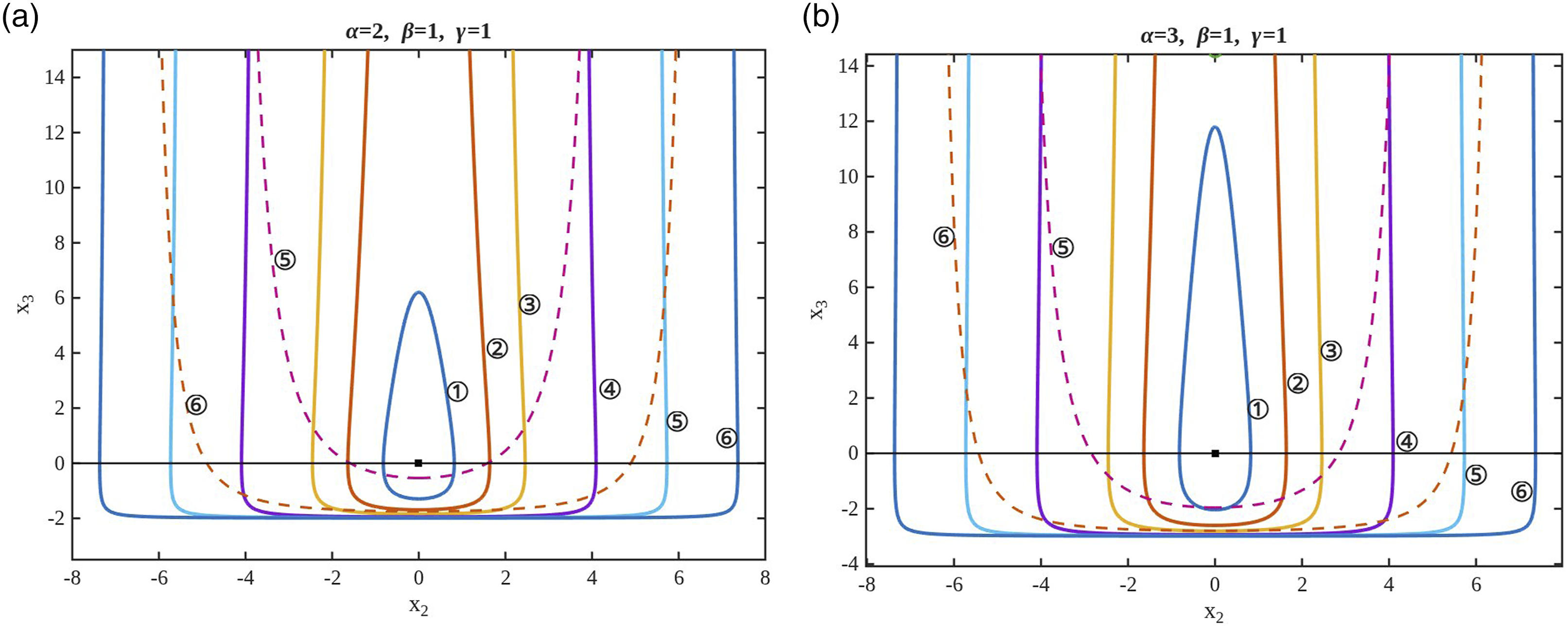
The W₁ represented by the solid line forms an oval-shaped curve, while upon reaching the singular point τ_s, the W₂ diffracted wavefront (dashed line) arises from infinity and evolves into super-elliptic form. Therefore, the two wavefronts propagating in the inhomogeneous anisotropic medium are present after τ_s. The other singular point of the ode is x₃ = −α/β never reached.

The wavefront behavior illustrated in the figures may appear counterintuitive, particularly due to the emergence of a secondary wavefront seemingly originating from infinity. However, this does not violate causality, since the analytical solution is governed by Heaviside functions that ensure the displacement field remains zero before the arrival of the wavefront and becomes nonzero only after the corresponding arrival time. Physically, this phenomenon arises in strongly inhomogeneous media, where the wave velocity varies significantly with depth.

5.1. Description of model parameters

The motivation to study the parameters α, β, γ, and ν is essentially performed to understand how material gradation influences wave propagation in functionally graded media. These parameters are not merely mathematical constants but represent physically controllable features in engineered materials.

1. α (Surface property parameter): This represents the baseline value of the material at the depth/surface (usually at x₃ = 0) and therefore controls the initial stiffness level of the material.

2. β (gradation rate parameter): This represents how quickly properties (elastic moduli) change along the depth coordinate x₃. The large β means that the material transitions from one state to another state vary rapidly over a short distance(more pronounced inhomogeneity in the medium).

3. γ (Scaling factor parameter): This acts as a scaling factor and determines the overall magnitude of the material property in the medium.

4. ν (shape parameter): This is the exponent of the power-law variation and therefore controls the smoothness or nonlinearity of the gradation profile.

Variations in these parameters affect the material gradation profile, which affects the geometry of the wavefront and the propagation pattern as depicted in the graphs (1–8). Larger values in these gradation factors result in more pronounced variations in material stiffness, which subsequently cause noticeable variations in the wavefront shape.

5.2. Numerical data used for plots

The parameters of the power-law gradation function vary for the simulation to investigate how they affect wave propagation. Gradation parameters α, β, γ are taken into account within the range 1 ≤ α ≤ 3, 1 ≤ β ≤ 3, 1 ≤ γ ≤ 3. This range represents moderate variations in the material gradation. One parameter varies within this range while the other two remain unchanged in order to examine the impact of each parameter independently. This allows feasible to compare the effects of each gradation parameter on how gradation influences how anti-plane SH waves propagate in the functionally graded material.

5.2.1. Effect of α (Figures 1, 2, 5 and 6)

Figures 1 and 2 correspond to ν = 1/5 with fixed β = γ = 1, while α varies from 1 to 3. An increase in α effectively shifts the material profiles through the factor (α + βx₃), resulting in a downward translation of the wavefronts along the depth direction. Both the wavefronts are extended towards the x₃ direction, denoting an increased depth-dependent propagation. The fundamental wavefront W₁ maintains an oval-like shape at early times, whereas the secondary diffracted front W₂ emerging after the critical time τ_s, expands more predominantly as α increases. A quite similar trend has been observed in Figures 5 and 6 for ν = 2. However, for the larger value of ν, the wavefronts show an impactful vertical stretching and decreased lateral spread, reflecting a stronger sensitivity of the wave kinematics to depth-dependent velocity variation.

5.2.2. Effect of β (Figures 3 and 7)

Figures 3 (ν = 1/5) and 7 (ν = 2) explain the impact of the gradient parameter β, which controls the rate of material variation with depth. When increasing the value of β, it leads to steeper wavefronts with reduced horizontal stretch and increased curvature toward the x₃ direction. This behaviour is attributed to stronger inhomogeneity gradients, which makes the wave trajectories bend and promote vertical focusing. The effect is more effective for ν = 2, where both W₁ and W₂ display sharper curvature and increased confinement along the depth direction.

5.2.3. Effect of γ (Figures 4 and 8)

Figures 4 (ν = 1/5) and 8 (ν = 2) demonstrate the importance of the scaling parameter γ, controlling the amplitude of the inhomogeneity function h (x₃). Increasing the value of γ exapnds the wave fronts in both horizontal as well as vertical direction uniformly, corresponding to an overall increase in wave speed. Despite this scaling effect, the qualitative strcuture of the wave fronts remains unchanged. The fundamental wavefront W₁ reaches infinity at the singular time τ_s, after which the secondary diffracted wavefront W₂ emerges and evolves into a super-elliptic shape.

The numerical simulations in Figures 1 –8 clearly shows that α primalily induces vertical shifting and stretching of wavefronts, β governs curvature and depth focusing through material gradients, and γ scales the propagation speed without altering the fundamental topology of the wavefronts. Furthermore, on comparing ν = 1/5 and ν = 2, it has been observed that smaller ν leads to flatter and laterally spread wavefronts, while larger ν produces highly elongated depth-dominated propagation patterns. It endorses the fact that the coupling between power-law velocity variation and SH-wave kinematics in functionally graded media is strong.

6. Conclusions

The article presents an analytical formulation for transient anti-plane (SH) wave propagation in transversely isotropic functionally graded media with depth-dependent power-law velocity variation. By considering independent inhomogeneity profiles for elastic moduli and mass density, a generalized Green’s function is derived, thereby extending earlier models restricted to identical grading laws.

Using integral transform techniques, closed-form expressions for the Green’s functions and the associated wavefront equations are obtained. The analysis reveals the existence of multiple wavefronts and provides insight into their evolution in graded anisotropic media.

The salient features of the present study are as follows:

• Existence of two distinct wavefronts: a primary outward-propagating front reaching infinity at a critical time, followed by a secondary diffracted front emerging from infinity, characteristic of inhomogeneous media.

• Clear identification of the role of inhomogeneity parameters: α induces vertical shifting and stretching of wavefronts, β governs curvature and depth focusing, γ scales wave speed without altering wavefront topology, and the power-law index ν controls lateral versus depth-dominated propagation.

• Development of exact closed-form Green’s function solutions, providing rigorous analytical benchmarks for complex inhomogeneous anisotropic media.

• The outcome of the current study has potential applications in seismic analysis, elastography, non-destructive evaluation, and the design of functionally graded materials with tailored wave propagation characteristics.

The present model can be extended in several directions. It may be generalized to multilayered functionally graded media by incorporating interface conditions to study wave transmission and reflection. The inclusion of nonlinear effects would allow analysis of amplitude-dependent wave behavior in soft materials. The framework can also be extended to coupled P-SV wave systems in anisotropic graded media. Furthermore, the analytical solutions developed here can serve as benchmark results for validating numerical methods and may be useful for future experimental studies in wave-based sensing and elastography.

Footnotes

ORCID iD

Sumit Kumar Vishwakarma

Funding

The authors received no financial support for the research, authorship, and/or publication of this article.

Declaration of conflicting interests

The authors declared no potential conflicts of interest with respect to the research, authorship, and/or publication of this article.

References

Abraham

(1982) Exact solutions of the one-dimensional acoustic wave equations for several new velocity profiles: transmission and reflection coefficients. Journal of the Acoustical Society of America 71(6): 1391–1399. https://doi.org/10.1121/1.387833

Bateman

Erdélyi

Magnus

, et al. (1954) Tables of Integral Transforms. McGraw-Hill, Vol. 1.

Benech

Brum

Grinspan

, et al. (2017) Analysis of the transient surface wave propagation in soft-solid elastic plates. Journal of the Acoustical Society of America 142(5): 2919–2932. https://doi.org/10.1121/1.4993633

Benech

Camargo

Negreira

(2022) Simplified green’s function for surface waves in quasi-incompressible elastic plates with application to elastography. Journal of Physics: Condensed Matter 34(21): 214004. https://doi.org/10.1088/1361-648x/ac5993

Chaudhary

Saeed

Singhal

(2025) Wave scattering and dynamic stress concentration in piezoelectric half-planes with semi-elliptical notches under sh-wave excitation. The European Physical Journal Plus 140(9): 852. https://doi.org/10.1140/epjp/s13360-025-06800-4

Chen

Cao

(2020) Green’s function for three-dimensional elastic wave equation with a moving point source on the free surface with applications. Geophysical Prospecting 68(4): 1281–1290. https://doi.org/10.1111/1365-2478.12928

Chew

(1995) Waves and Fields in Inhomogeneous Media. IEEE Press.

Daros

(2008) A fundamental solution for sh-waves in a class of inhomogeneous anisotropic media. International Journal of Engineering Science 46(8): 809–817. https://doi.org/10.1016/j.ijengsci.2008.02.001

Daros

(2009) A time-harmonic fundamental solution for a class of inhomogeneous transversely isotropic media. Wave Motion 46(4): 269–279. https://doi.org/10.1016/j.wavemoti.2009.02.001

10.

Daros

(2013) Green’s function for sh-waves in inhomogeneous anisotropic elastic solid with power-function velocity variation. Wave Motion 50(2): 101–110. https://doi.org/10.1016/j.wavemoti.2012.07.004

11.

Debnath

Bhatta

(2011) Integral Transforms and Their Applications. Chapman and Hall/CRC.

12.

Hemalatha

Kumar

Ahamad

, et al. (2025) Effect of point source on the sh wave propagation in a functionally graded piezoelectric structure: green’s function approach. Mechanics of Solids 60: 1–16. https://doi.org/10.1134/s0025654425602952

13.

Hook

(1962) Green’s functions for axially symmetric elastic waves in unbounded inhomogeneous media having constant velocity gradients. Journal of Applied Mechanics 29(2): 293–298.

14.

Kumawat

Vishwakarma

(2025a) Reflection–transmission coefficients of sh waves across thin-walled spring-membrane strain gradient interface. European Journal of Mechanics - A: Solids 111: 105531. https://doi.org/10.1016/j.euromechsol.2024.105531

15.

Kumawat

Vishwakarma

(2025b) Reflection-transmission coefficient of sh waves in a layered interface with spring sandwiched between thin membranes: an application of strain gradient theory. Mechanics of Advanced Materials and Structures 33: 1–11. https://doi.org/10.1080/15376494.2025.2467238

16.

Kumawat

Kumar Vishwakarma

Touhei

(2025a) Dispersive constraints of antiplane shear waves in a strain-gradient loh model under an inflexible boundary plane and initial pressure. International Journal of Geomechanics 25(3): 04024360. https://doi.org/10.1061/ijgnai.gmeng-9605

17.

Kumawat

Praharaj

Vishwakarma

(2025b) Dispersion of torsional surface waves in a threefold concentric compounded cylinder with imperfect interface. Waves in Random and Complex Media 35(6): 11223–11248. https://doi.org/10.1080/17455030.2022.2121012

18.

Kumhar

Kundu

Pandit

, et al. (2020) Green’s function and surface waves in a viscoelastic orthotropic FGM enforced by an impulsive point source. Applied Mathematics and Computation 382: 125325. https://doi.org/10.1016/j.amc.2020.125325

19.

Manolis

Karakostas

(2003) A green’s function method to sh-wave motion in a random continuum. Engineering Analysis with Boundary Elements 27(2): 93–100. https://doi.org/10.1016/s0955-7997(02)00086-3

20.

Manolis

Shaw

(1996) Green’s function for the vector wave equation in a mildly heterogeneous continuum. Wave Motion 24(1): 59–83. https://doi.org/10.1016/0165-2125(96)00006-6

21.

Mistri

Dholey

Vishwakarma

, et al. (2026) Influence of dual electric membranes pairing with a sandwiched electrically induced spring interface on sh-wave propagation in smart porous composite. Journal of Vibration Engineering & Technologies 14(4): 176. https://doi.org/10.1007/s42417-026-02411-0

22.

Morse

Feshbach

(1953) Methods of Theoretical Physics. McGraw-Hill.

23.

Oberhettinger

(1958) On the diffraction and reflection of waves and pulses by wedges and corners. Journal of Research of the National Bureau of Standards 61(5): 343–365. https://doi.org/10.6028/jres.061.030

24.

Oberhettinger

Badii

(2012) Tables of Laplace Transforms. Springer Science & Business Media.

25.

Panigrahi

Kumawat

Vishwakarma

(2025) A case-based study of corrugated boundaries in a trilayered structure and their influence on lt waves. International Journal of Geomechanics 25: 113–129. https://doi.org/10.1061/ijgnai.gmeng-10266

26.

Payton

(2012) Elastic Wave Propagation in Transversely Isotropic Media. Springer Science & Business Media, Vol. 4.

27.

Rangelov

Manolis

Dineva

(2005) Elastodynamic fundamental solutions for certain families of 2d inhomogeneous anisotropic domains: basic derivations. European Journal of Mechanics - A: Solids 24(5): 820–836. https://doi.org/10.1016/j.euromechsol.2005.05.002

28.

Restrepo

Gómez

JDJ

Jaramillo

(2014) Sh wave number green’s function for a layered, elastic half-space. Part I: theory and dynamic canyon response by the discrete wave number boundary element method. Pure and Applied Geophysics 171: 2185–2198. https://doi.org/10.1007/s00024-014-0780-4

29.

Singh

Das

Mistri

, et al. (2017) Green’s function approach to study the propagation of sh-wave in piezoelectric layer influenced by a point source. Mathematical Methods in the Applied Sciences 40(13): 4771–4784. https://doi.org/10.1002/mma.4343

30.

Sneddon

(1972) The Use of Integral Transforms. McGraw-Hill.

31.

Watanabe

(1982) Transient response of an inhomogeneous elastic solid to an impulsive sh-source: variable sh-wave velocity. Bulletin of JSME 25(201): 315–320. https://doi.org/10.1299/jsme1958.25.315

32.

Watanabe

Payton

(1997) Sh wave in a cylindrically anisotropic elastic solid a general solution for a point source. Wave Motion 25(2): 197–212. https://doi.org/10.1016/s0165-2125(96)00041-8

33.

Watanabe

Payton

(2004) Green’s function and its non-wave nature for sh-wave in inhomogeneous elastic solid. International Journal of Engineering Science 42(19-20): 2087–2106. https://doi.org/10.1016/j.ijengsci.2004.08.001

34.

Zaitsev

Polyanin

(2002) Handbook of Exact Solutions for Ordinary Differential Equations. Chapman and Hall/CRC.