
Abstract
To solve the problem of low accuracy in fault diagnosis caused by insufficient feature extraction of gear vibration signals, this paper sets forth a gear fault diagnosis method based on cross-attention fusion and establishes a CNN-BiTCN-CA diagnosis model. The original signal is reconstructed using variational mode decomposition (VMD) and fast Fourier transform (FFT). Time-frequency features are extracted using a bidirectional temporal convolutional network (BiTCN) and a convolutional neural network (CNN), respectively. The cross-attention mechanism (CA) is then utilized to fuse these time-frequency features, enabling comprehensive extraction of the original signal’s fault characteristics. Finally, a fully connected layer is employed to achieve accurate diagnosis of gear fault types. The experimental study demonstrates that in a Gaussian white noise environment with a signal-to-noise ratio (SNR) of 7.08 dB, the CNN-BiTCN-CA model achieves a gear fault classification accuracy of 99.85%. When Gaussian white noise with a SNR of 1.77 dB is introduced, the proposed model still achieves a diagnostic accuracy of 95.82%. The CNN-BiTCN-CA model is capable of extracting fault features in depth from the gear signal and effectively improving fault classification accuracy.
Keywords
1. Introduction
In the realm of mechanical engineering, toothed gear transmission serves as a key component of machinery systems. Within contemporary industrial and engineering sectors, it plays a pivotal role. The efficient and reliable operation of gears directly affects the overall performance and service life of the host mechanical system (Jiang et al., 2013). However, gears are susceptible to predominant failures during operation, such as surface pitting, root cracks, and tooth breakage. If these issues are left undetected and unaddressed, they can lead to potential safety hazards in the machinery, resulting in significant economic losses and severe mechanical failures. Therefore, detecting gear operational status and diagnosing performance degradation early are essential for achieving fault classification and root cause analysis. This capability is crucial for advancing industrial intelligence and is essential for ensuring the operational safety and reliability of machinery (Lei et al., 2013).
As an essential component of smart manufacturing, data-driven intelligent fault diagnosis, characterized by its efficient processing of vast equipment condition data, has become a focal research direction in the application of big data technologies for advanced diagnostics of critical equipment (Li et al., 2022). Due to operational environmental influence, gear vibration signals acquired by sensors are often disrupted by multi-source excitations, response coupling, and strong ambient noise. This leads to pronounced nonlinearity and non-stationarity in the collected signals, thereby increasing the complexity of extracting fault information from the vibration signals (Chen et al., 2025). To achieve precise recognition of both subtly different single fault modes and their severity levels across various fault classes, innovative methodologies enabling automated feature extraction and diagnosis are imperative. Deep learning models can automatically uncover essential features from vibration signals. Compared to conventional gear fault diagnosis methods, they not only reduce manual intervention but also demonstrate superior performance in classification tasks, making them a rapidly emerging hotspot in intelligent fault diagnosis (Lei et al., 2018).
Convolutional neural networks (CNNs), as one of the pivotal models in deep learning, have attracted considerable attention within the gear fault diagnosis community, drawing significant interest from both domestic and international experts and scholars. Sadoughi and Hu (2019) proposed a method that integrates CNN and VMD to implement fault diagnosis across different fault categories. Hashim and Kumar et al. (2025) proposed using the Energy Operator variant EO123 for signal preprocessing, achieving significantly improved CNN accuracy in gearbox fault diagnosis. Xu et al. (2026) proposed a self-supervised learning model, TFDDP, based on time-frequency dual-domain prediction, which achieved promising diagnostic performance under different operating conditions and limited labeled samples. He et al. (2026) proposed a self-supervised learning model, TFDDCF, based on time-frequency dual-domain contrast and fusion, which achieved excellent fault diagnosis performance under limited labeled samples.
Among various deep learning technologies, the attention mechanism, as a significant advancement in recent years, dynamically adjusts the model’s focus across different regions or time steps, thereby effectively extracting and utilizing critical feature information (Vaswani et al., 2017). Chen et al. (2025) proposed a novel approach based on a multi-path CNN and a dual-branch attention mechanism (AMPCNN). This method employs multi-path convolution to distill multi-scale features from vibration signals and incorporates an attention mechanism to amplify the recognition capability for various categories of faults. Zhou et al. (2024) investigated a novel fault diagnosis methodology incorporating a frequency-aware attention mechanism within a convolutional neural network to enhance feature discrimination.
The aforementioned studies have shown that vibration-based fault diagnosis methods can effectively address gear fault classification issues under multiple operating conditions. Those approaches might fail to account for features from signal sources and simultaneously overlook the impact of backward information on prediction results. Sprangers et al. (2023) first introduced the bidirectional temporal convolutional network (BiTCN) model, which enhances computational accuracy by performing dual encoding operations on future and past data, thereby comprehensively capturing the bidirectional dependency relationships within the signal. Methods that integrate time-frequency information can effectively improve the accuracy of fault diagnosis tasks (Liang, 2026). Xu et al. (2026) developed a time-frequency fully connected graph neural network (TF-FC-GNN) that integrates dual-stream learning with a multi-graph strategy to fuse cross-domain features. Chen et al. (2025) proposed a time-frequency aware feature disentanglement (TFAFD) framework, employing collaborative dynamic convolution modules to capture non-stationary characteristics effectively. Additionally, other approaches generate time-frequency representations to support feature fusion in classification and diagnostic tasks. However, this approach of first generating 2D spectrograms and then performing classification often faces challenges such as high GPU utilization and prolonged training times (Akan and Cura, 2021).
To address the issue of insufficient feature extraction from gear vibration signals leading to low fault diagnosis accuracy, this work introduces a novel gear fault diagnosis model formulates a feature cross-attention mechanism fusion (CNN-BiTCN-CA). We established experimental signal reconstruction for gears, utilizing a BiTCN to extract time-domain features from vibration signals and CNN to acquire frequency-domain features from vibration signals. A cross-attention mechanism is then utilized to fuse the time-frequency features, and a fully connected layer is used to realize precise classification and diagnosis of gear fault types. Experimental results from gear fault simulation tests and supplementary experiments using the Southeast University Fault Dataset (SUFD) demonstrate that the integration of time-domain and frequency-domain features using the CNN-BiTCN-CA model can effectively enhance fault recognition accuracy.
2. Theoretical foundation
2.1. Convolutional neural network
CNN excel at mining spatial features from imagery and datasets, demonstrating superior performance in tasks related to feature identification and extraction. CNN is primarily composed of an input layer, convolutional layers, activation functions, pooling layers, and fully connected layers. The fundamental architecture of CNN is shown in Figure 1. Structure of CNN model.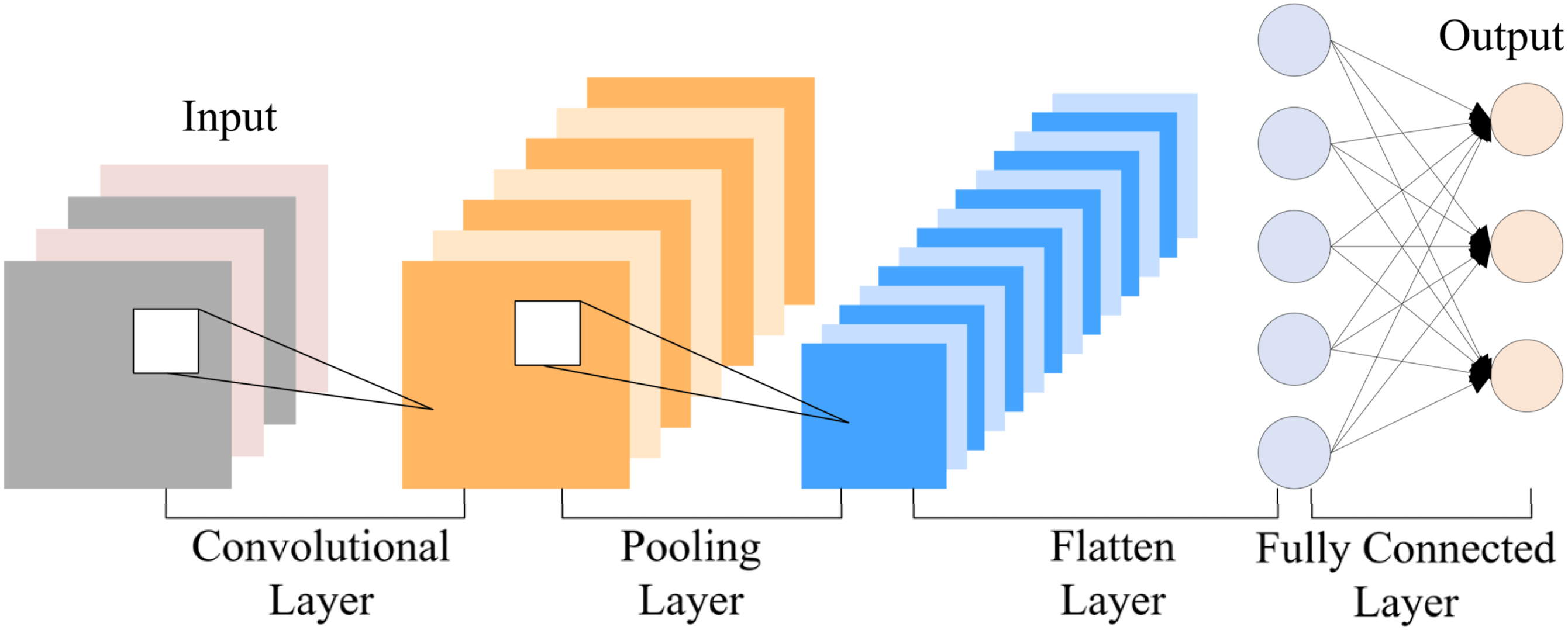
The convolutional layer performs convolution operations on the input data using convolutional kernels, thereby enabling feature extraction. The convolution operation is formulated as follows:
Upon the completion of the convolution operation, the ReLU (Rectified Linear Unit) activation function is applied:

The pooling layer performs feature dimensionality reduction. Its operation is defined as follows:

2.2. Bidirectional temporal convolutional network
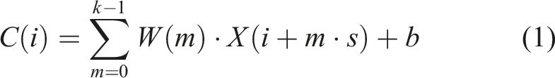
BiTCN is a deep learning model designed for time series analysis. This model combines the architectural framework of the temporal convolutional network (TCN) with a bidirectional processing mechanism. Traditional TCN only considers forward convolutional computations of the input sequence thereby neglecting the impact of backward information on prediction outcomes. The BiTCN architecture comprises two distinct TCN pathways: one dedicated to encoding future covariates, and the other to encoding past covariates along with the historical sequence values (Sprangers et al., 2023). Therefore, BiTCN can better capture the hidden features in time series data and speed up the model training process, as illustrated in Figure 2. Bidirectional temporal convolution network structure.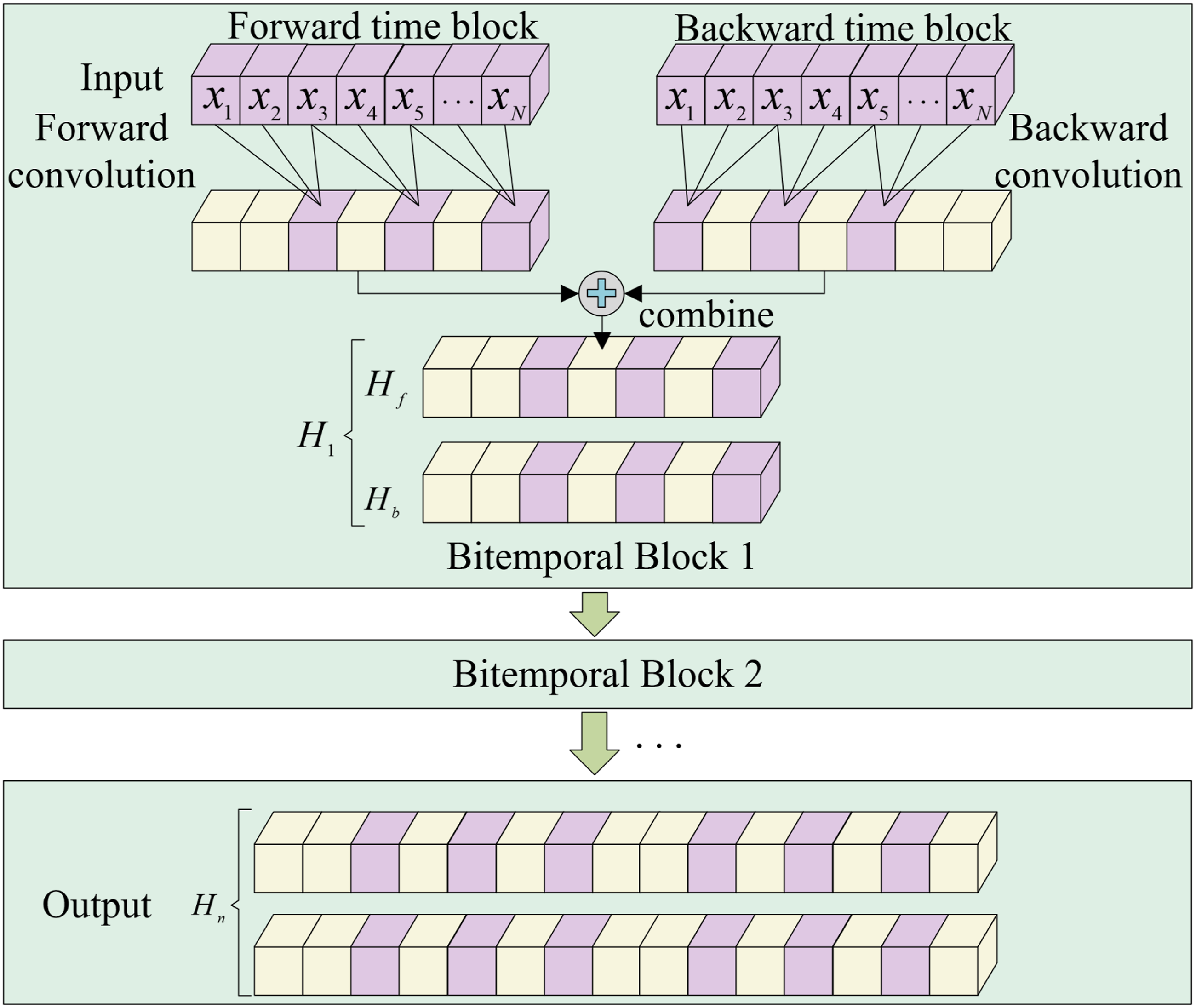
BiTCN consists primarily of multiple bitemporal blocks, each of which is detailed below.
The matrix for the input signal is: (1) Forward time block
A forward convolution operation is performed on the input signal, resulting in the output matrix (2) Backward time block

A backward convolution operation is performed on the input signal, resulting in the output matrix (3) Bitemporal block

The forward and backward time blocks jointly constitute the bitemporal block, merging the results of forward and backward convolutions:

Subsequently, multiple bitemporal blocks can be stacked together, with the result from the previous block serving as the input for the next block. Then, the output of the n-th layer bitemporal block is:

2.3. Cross-attention
Cross-attention mechanism is an innovative information processing method designed to establish attention connections between different modules or modalities, dynamically adjusting and integrating multi-source data information. Compared with the self-attention mechanism (SA), the cross-attention (CA) mechanism demonstrates significant advantages in diagnostic tasks. Specifically, CA facilitates the fusion of time and frequency features, models the interdependencies between them, and thereby leverages their complementary nature (Jian et al., 2024). By focusing on dynamic weights between different features, CA optimizes fault detection accuracy and dynamically adapts to the varying importance of features across different fault types. The schematic in Figure 3 illustrates the structure of the cross-attention mechanism. Cross-attention mechanism network structure.
The calculation process of cross-attention is as follows: (1) Input features:
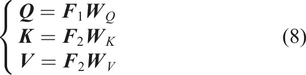
Vibration signals’ features extracted using different methods can be represented as matrices (2) Linear transformation
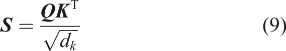
Map (3) Attention scores (S)
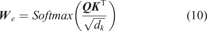
To evaluate the dot product of (4) Attention weights (
Apply the Softmax function to the scores for normalization, thereby obtaining the attention weights: (5) Cross-attention output (
Apply the obtained attention weight matrix to the value matrix

3. Construction of fault diagnosis model
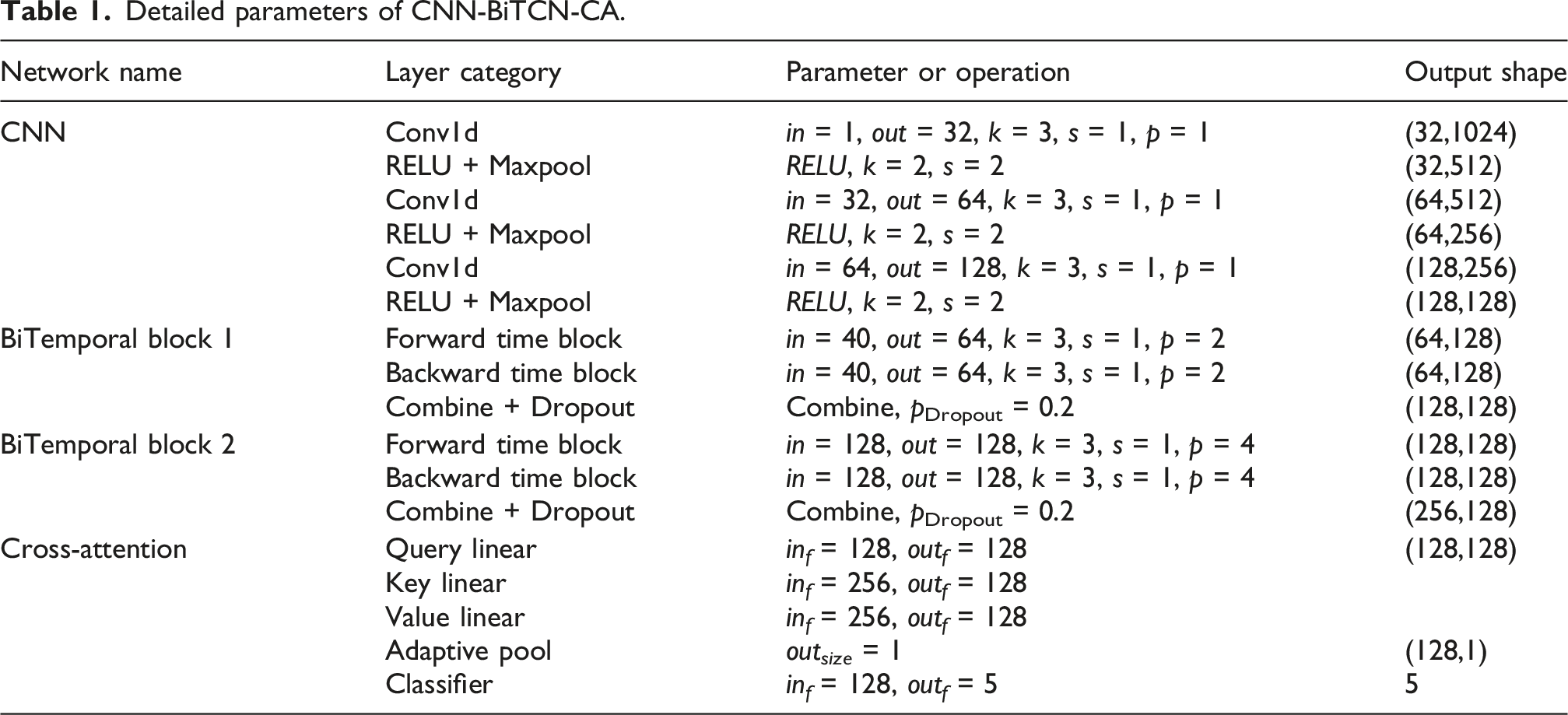
To address the problem of inadequate feature extraction from gear vibration signals, which leads to low fault diagnosis accuracy, this work introduces a gear fault classification method based on a cross-attention mechanism that fuses time-frequency features extracted by CNN and BiTCN (CNN-BiTCN-CA). First, frequency-domain features are extracted from the signal after fast Fourier transform (FFT), and time-domain features are extracted from the signal after variational mode decomposition (VMD). Subsequently, these time-frequency features are fused through a cross -attention module. Finally, fault type classification and diagnosis are performed through a fully connected layer. The overall process is illustrated in Figure 4. The configuration of the CNN-BiTCN-CA model is detailed in Table 1. Diagnosis process of the CNN-BiTCN-CA model. Detailed parameters of CNN-BiTCN-CA.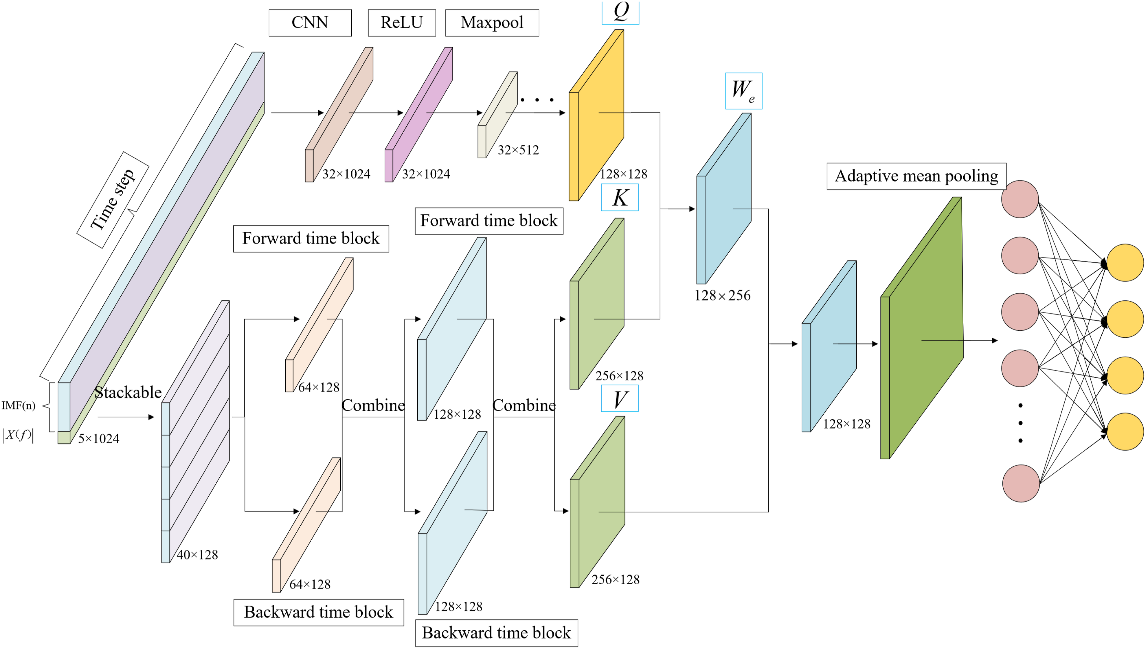
3.1. Feature dataset construction
Vibration signals are acquired from the spur gear fault simulation test bench and the SUFD. The SNR denotes the ratio of signal power to noise power, typically expressed in decibels (dB). The calculation procedure is as follows: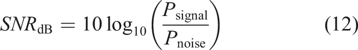
In the formula: Psignal represents the signal power; Pnoise represents the noise power. The smaller the SNR, the stronger the noise interference.
To simulate the signal complexity due to noise contamination in real-world environments, Gaussian white noise with an SNR of 7.08 dB is introduced into the vibration signal. This step is designed to validate the model’s feature extraction capability in practical environments (Han et al., 2022). A time-frequency analysis comparing the signals before and after the introduction of Gaussian white noise is provided, as shown in Figure 5. Comparison of time-frequency domain signals before and after the addition of Gaussian white noise.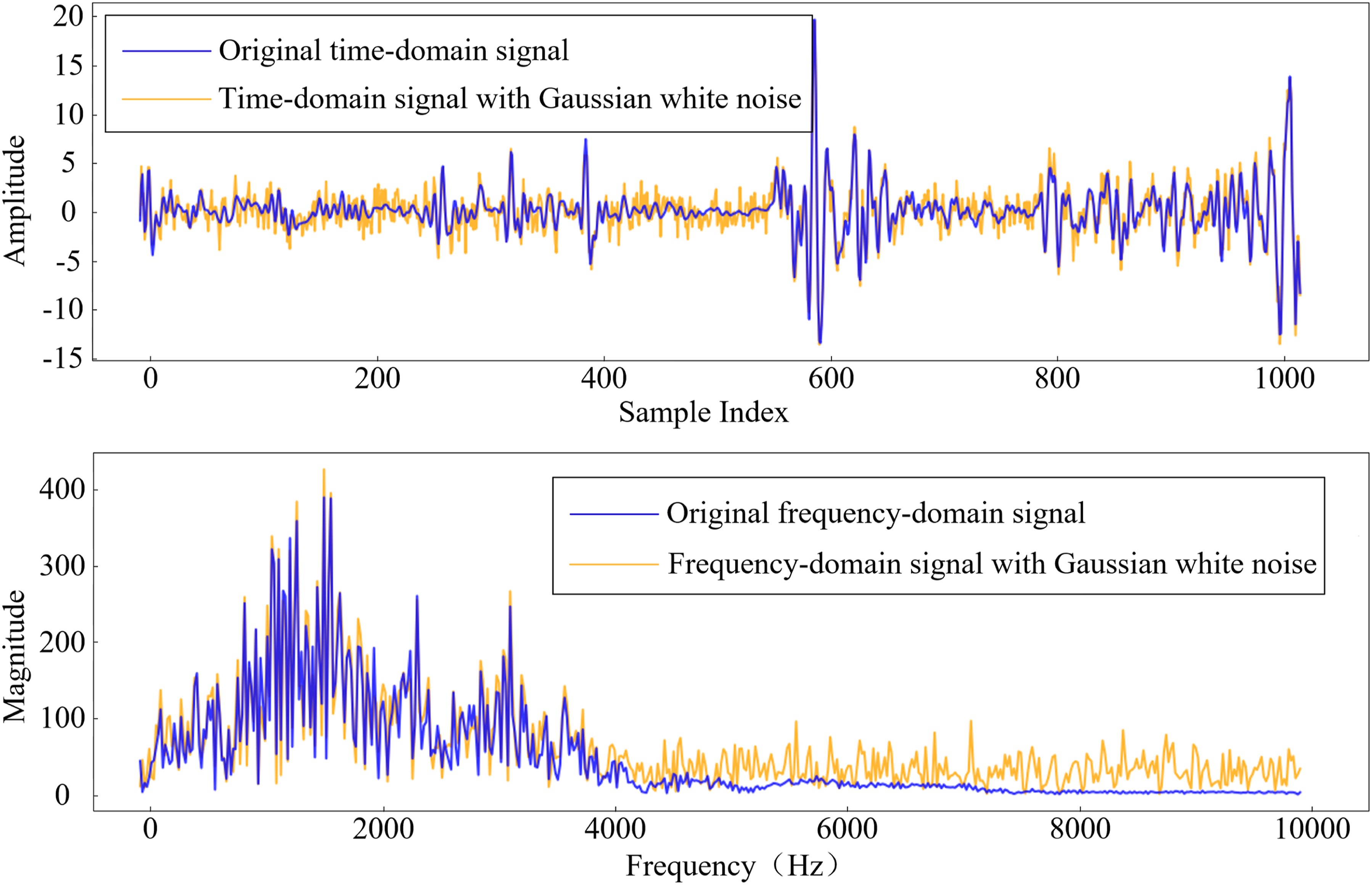
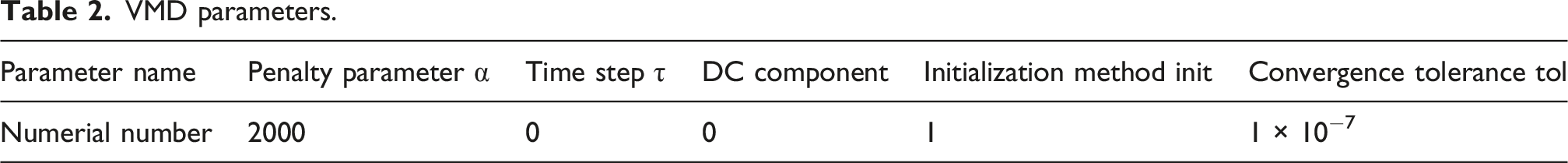
The vibration signals were segmented into samples using a sliding window with a length of 1024 and an overlap ratio of 50%. Based on the sampling frequency of 20 kHz and the rotational speed of 2000 r/min, each sample contained approximately 1.7 fault-response periods on average. Therefore, although adjacent samples overlapped in the time domain to a certain extent, they were not simple duplications of the same local fault feature. This method can preserve the integrity of fault information while effectively reducing the risk of sample redundancy caused by overlapping sampling. After random shuffling, the resulting samples were divided into training, test, and validation sets at a ratio of 7:1:2. To enhance fault features from the raw signal, time-frequency signals were obtained using both VMD (Fan et al., 2025) and fast Fourier transform (FFT). The process for constructing the feature dataset is illustrated in Figure 6. Feature dataset production.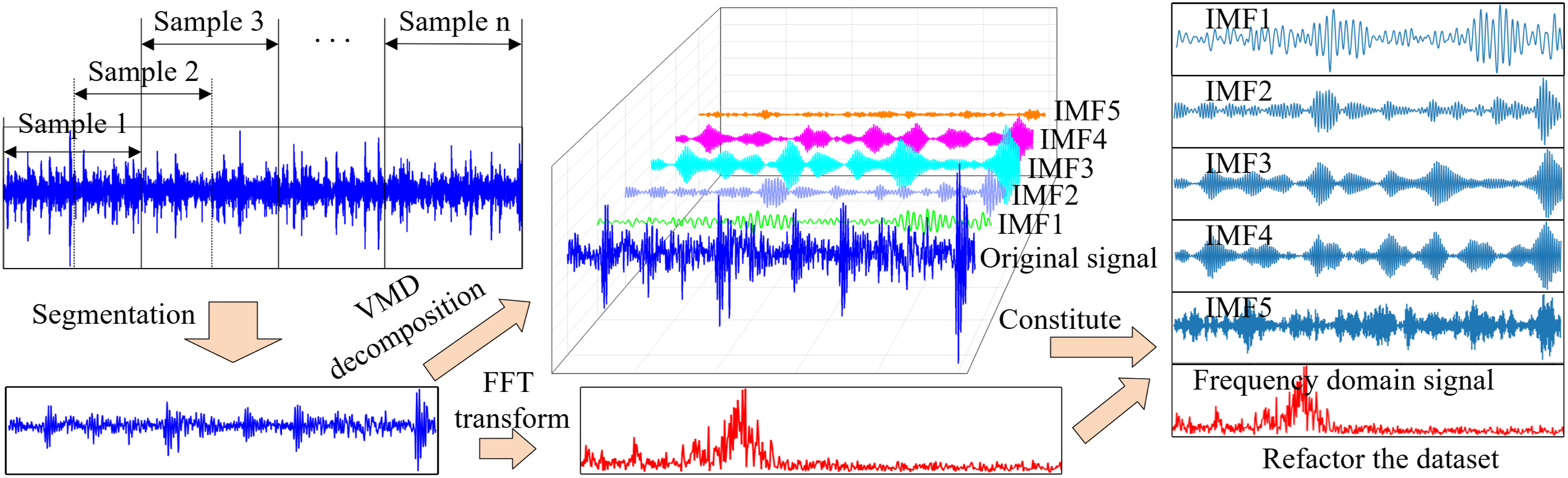
Apply the VMD method to decompose discrete-time domain signals x[n]. 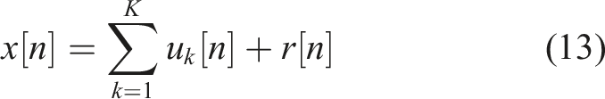
VMD parameters.
Apply FFT to obtain the frequency-domain signal.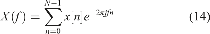
Obtain the magnitude spectrum│X (f)│.
In the equation, Re(X ( f) ) and Im(X ( f) ) represent, respectively, the real part and the imaginary part of X (f).
The five IMFs components obtained from each 1024-point sample were stacked along the channel dimension to form a multichannel time-domain feature matrix
3.2. Feature extraction, fusion, and classification process
Considering the bidirectional dependencies in time-domain features and the complex information encompassed by frequency-domain features, the CNN-BiTCN-CA model is employed to perform deep extraction and fusion of fault features. Subsequently, a fully connected layer is utilized to for the classification and diagnosis of fault types.
The frequency-domain signal from the reconstructed signal is input into a network consisting of three CNN layers to extract frequency-domain features, as shown in Figure 7. CNN extract frequency-domain features.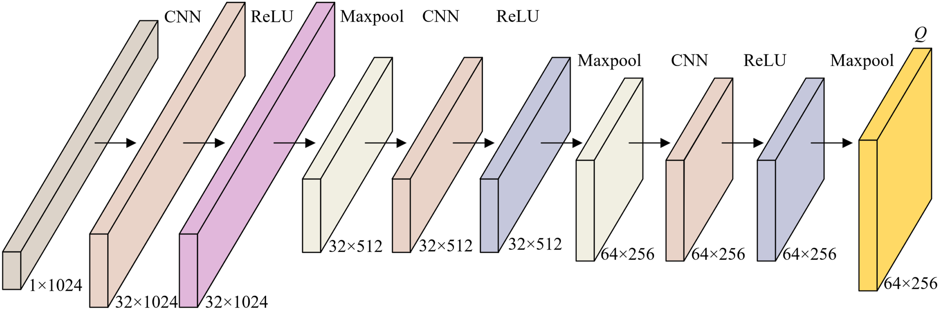
The multiple modal signals from the reconstructed signal are stacked and input into the BiTCN module to extract time-domain features. Within each bitemporal block stage, the forward temporal block and the backward temporal block have identical network structures, as illustrated in Figure 8. Structure diagram of BiTCN time blocks.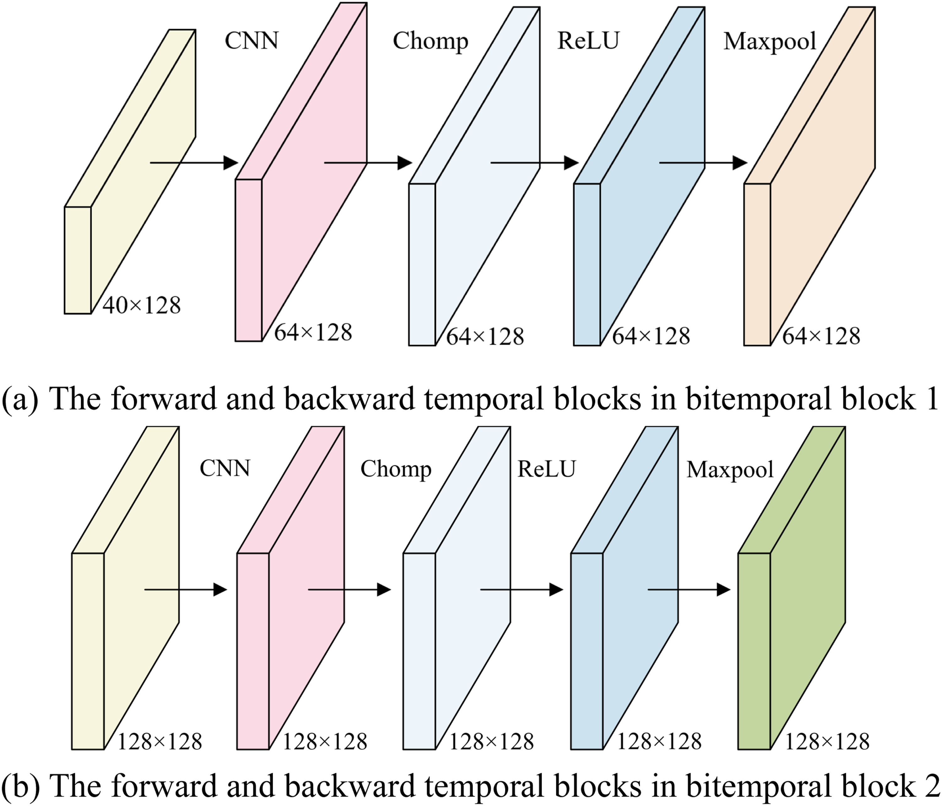
The feature matrices
4. Experimental setup and data acquisition
To verify the accuracy of the CNN-BiTCN-CA model in classifying different gear faults under strong interference environments, simulated fault experiments on spur gears were conducted with the support of the National-Local Joint Engineering Research Center. Additionally, supplementary validation was carried out using the well-established SUFD.
4.1. Spur gear simulated fault test rig
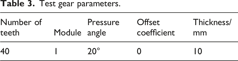
Test gear parameters.
To simulate gear faults, various methods were applied to process gears at different positions. Linear cutting is used to create crack faults; non-uniform small pits are processed on the tooth surface to simulate pitting faults, and linear cutting is used to fabricate broken and missing tooth faults, respectively. Additionally, a fault-free type is included for comparison. A total of five different types of test gears are generated.
The DH5922N dynamic signal testing and analysis system and the DH311E accelerometer were employed to acquire the vibration signals of the test gears. The sampling rate is set to 20 kHz, and the stable rotational speed of the shaft with the faulty gear is 1000 r/min. Vibration signal tests are conducted on both healthy gears and the four distinct types of faulty test gears. The spur gear fault simulation test rig primarily is composed of a drive motor, a speed controller, a gear reducer, a coupling, test gears, a simulated load, an accelerometer, a data acquisition system, and a digital display computer. The gear fault simulation test site and labels for various faulty gears are presented in Figure 9. Gear fault simulation test site and labels for various faulty gears.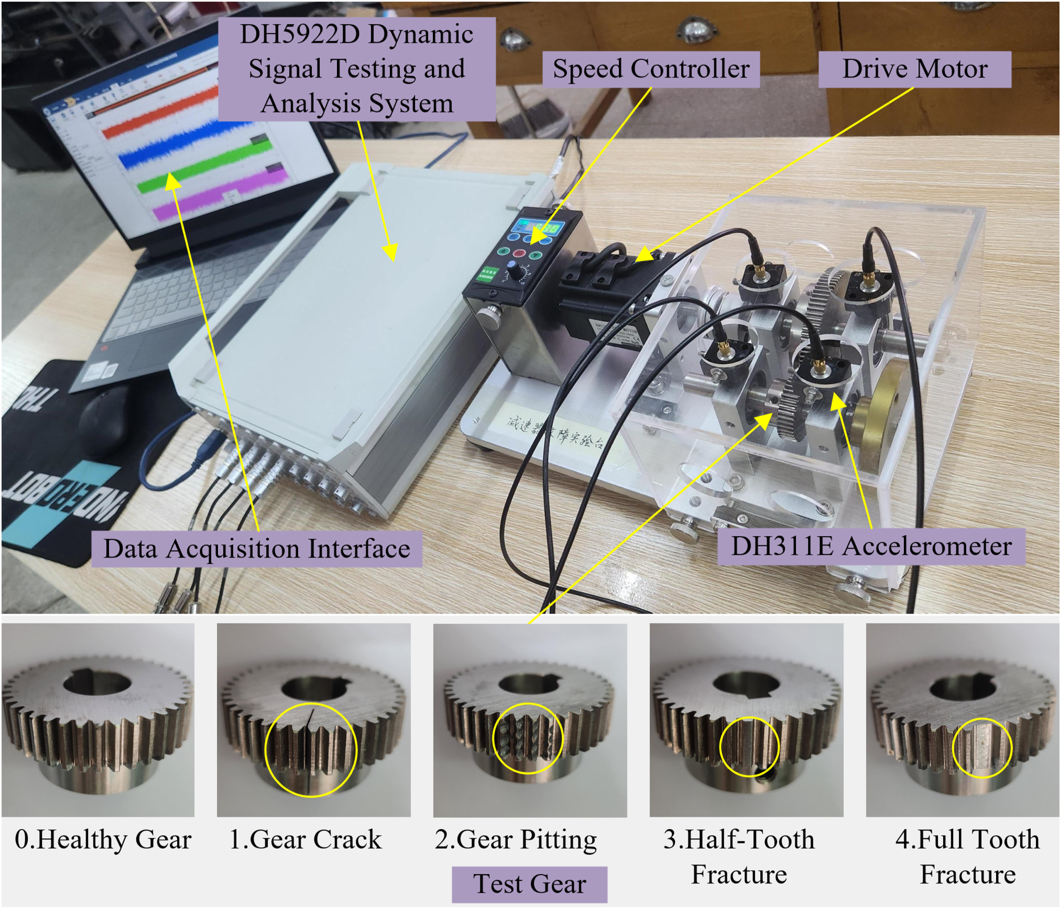
4.2. The Southeast University fault dataset
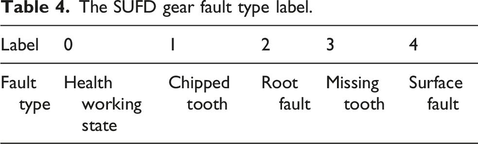
The publicly available spur gear fault dataset from Southeast University has shown extensive applicability and has made a significant impact in the field of fault diagnosis. To validate the accuracy of the CNN-BiTCN-CA and research findings presented in this paper, the SUFD spur gear dataset is utilized as supplementary experiments. The SUFD experimental setup is shown in Figure 10. SUFD fault simulation test bench.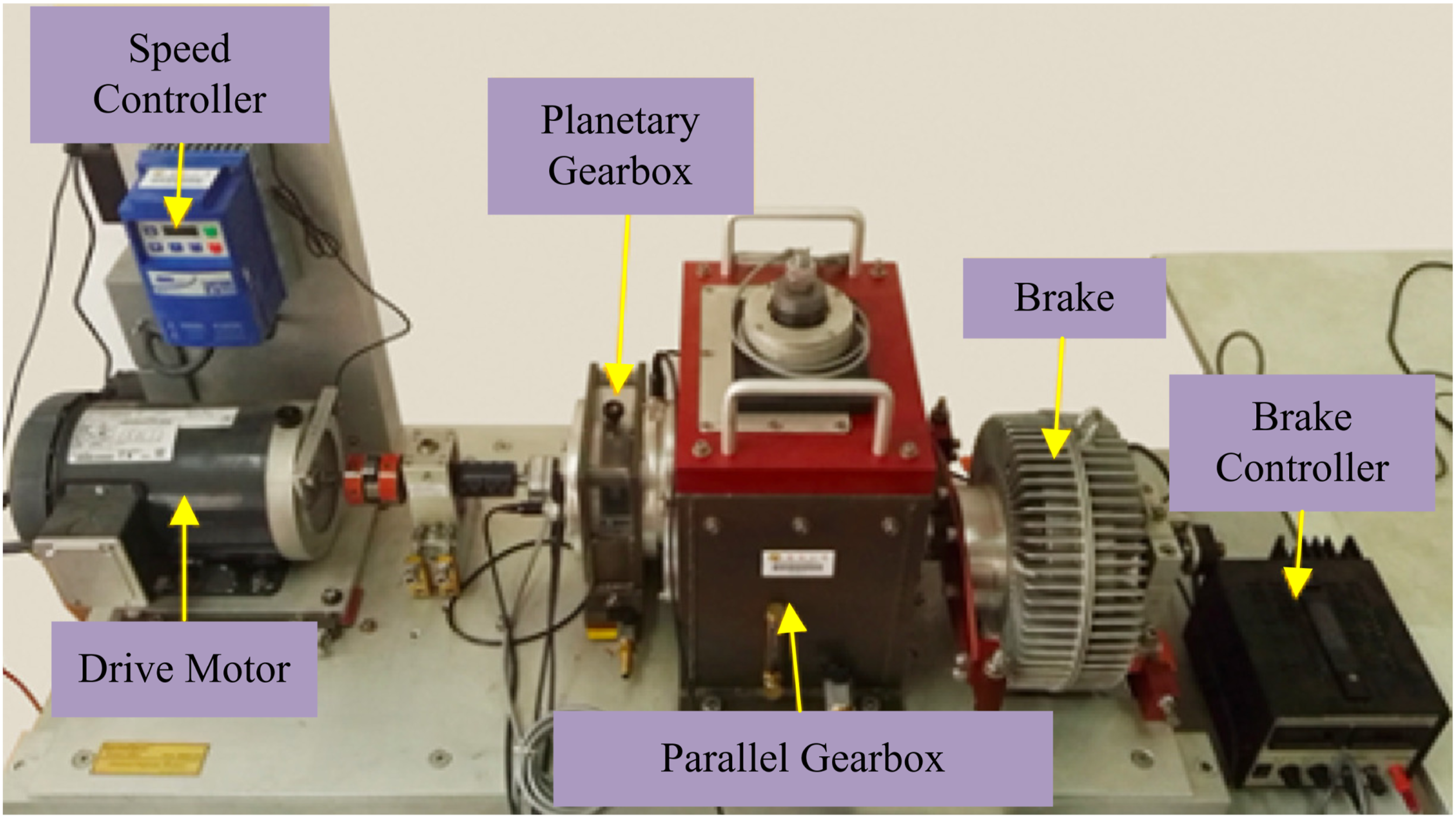
The SUFD gear fault type label.
5. Experimental results and analysis
5.1. Training and testing results analysis
To evaluate the accuracy of the CNN-BiTCN-CA method for gear fault diagnosis, a simulated experimental dataset was utilized to conduct the model’s performance training and testing. The training parameters were set as follows: 20 epochs, a batch size of 32, and a learning rate of 0.0003. The testing was conducted on a computer running Windows 11 (64-bit), with CUDA 12.5. The models were implemented in Python 3.9.11 using the PyTorch deep learning framework. The hardware specifications included an Intel Core i5-13490F CPU, an RTX 4070 Ti Super GPU, and.
The comparative performance of the methods was evaluated using the F1-score. The F1 metric takes into account both the precision and recall of the classification models. If the prediction performance on the test feature samples is better, the F1 value will be larger; conversely, it will be smaller (Takahashi et al., 2024). The F1-score is calculated as follows: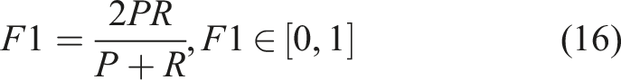
To validate the superiority of the proposed CNN-BiTCN-CA model for gear fault diagnosis, comparative analyses were conducted under identical data preprocessing conditions. Frequency-domain signals obtained via FFT were input into CNN-SA, and CNN models for comparison. Time-domain signals derived from VMD preprocessing were fed into BiTCN models for comparison. The input for the CNN-LSTM model was constructed by concatenating frequency-domain signals from FFT with time-domain signals derived from VMD. The CNN and BiTCN models share identical architectural configurations with the corresponding branches in the proposed CNN-BiTCN-CA framework. Under the condition of retaining the original branches of CNN-BiTCN-CA, replace the final cross-attention mechanism module with a feature concatenation operation to obtain the CNN-BiTCN model (Figure 11). Compare CNN-BiTCN-CA with other classification models.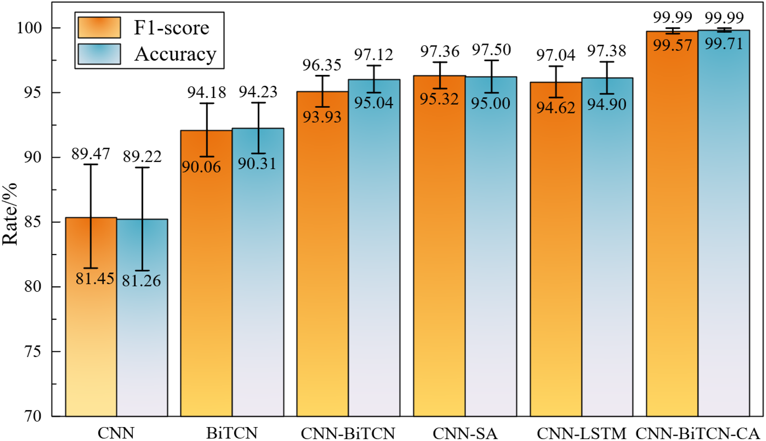
The CNN-BiTCN-CA model demonstrates superior performance in classification tasks, with accuracy and F1-score both nearing 100%. This indicates the model’s ability to accurately detect and cover all categories of gear faults. The training results demonstrate that the CNN-BiTCN -CA model is fully capable of effectively handling various gear fault classification tasks. The training comparison results reveal that the CNN-BiTCN-CA model exhibits superior performance metrics for gear fault classification tasks, with training accuracy improved by approximately 14.61%, 7.58%, 3.77%, 3.60%, and 2.74% compared to CNN, BiTCN, CNN-BiTCN, CNN-SA, and CNN-LSTM, respectively. These results indicate that the method of integrating time-frequency features via a cross-attention mechanism can effectively capture gear fault characteristics, thereby significantly improving the accuracy of fault classification.
Identification accuracy in different SNR environments.
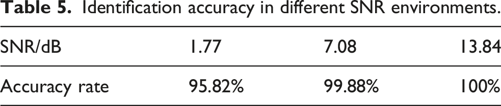
As shown in Tables 5, it can be observed that when Gaussian white noise with a SNR of 13.84 dB is introduced, the model records an accuracy of 100% in gear fault identification. Furthermore, when Gaussian white noise with a SNR of 7.08 dB is introduced, the model maintains a high accuracy of 99.88%. Even when Gaussian white noise with a SNR of 1.77 dB is introduced, the model still achieves an impressive accuracy of 95.82%. These results robustly demonstrate the high accuracy and effectiveness of the CNN-BiTCN-CA model in identifying gear fault types.
To validate the stability and effectiveness of the CNN-BiTCN-CA model in gear fault classification diagnosis, training and testing curves were presented in Figure 12. Train and test curves.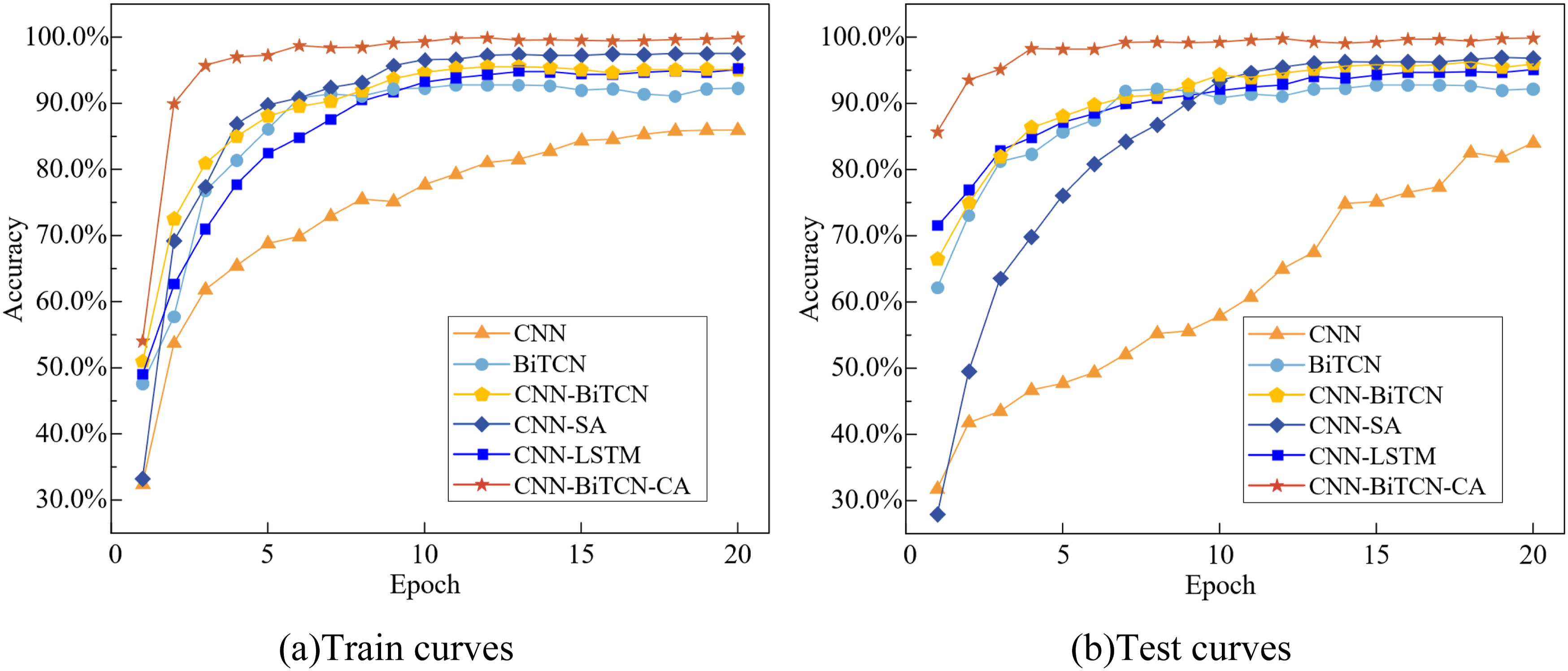
Figure 12 demonstrates the CNN-BiTCN-CA model achieved an accuracy of over 95% at the 5th iteration and maintained a stable accuracy above 99.5% in later iterations, with no signs of over fitting. In contrast, the CNN, BiTCN, CNN-BiTCN, CNN-SA, and CNN-LSTM models showed significantly slower convergence speeds compared to the CNN-BiTCN-CA model, and their classification diagnostic accuracy was below 98%, with instances of instability observed during iterations. The training and testing results demonstrate that the CNN-BiTCN-CA model exhibits excellent stability and effectiveness in diagnosing gear faults.
A confusion matrix was introduced for the comparative analysis of the diagnostic results from the gear fault simulated experiments, Figure 13 shows. Confusion matrix for the different diagnostic models.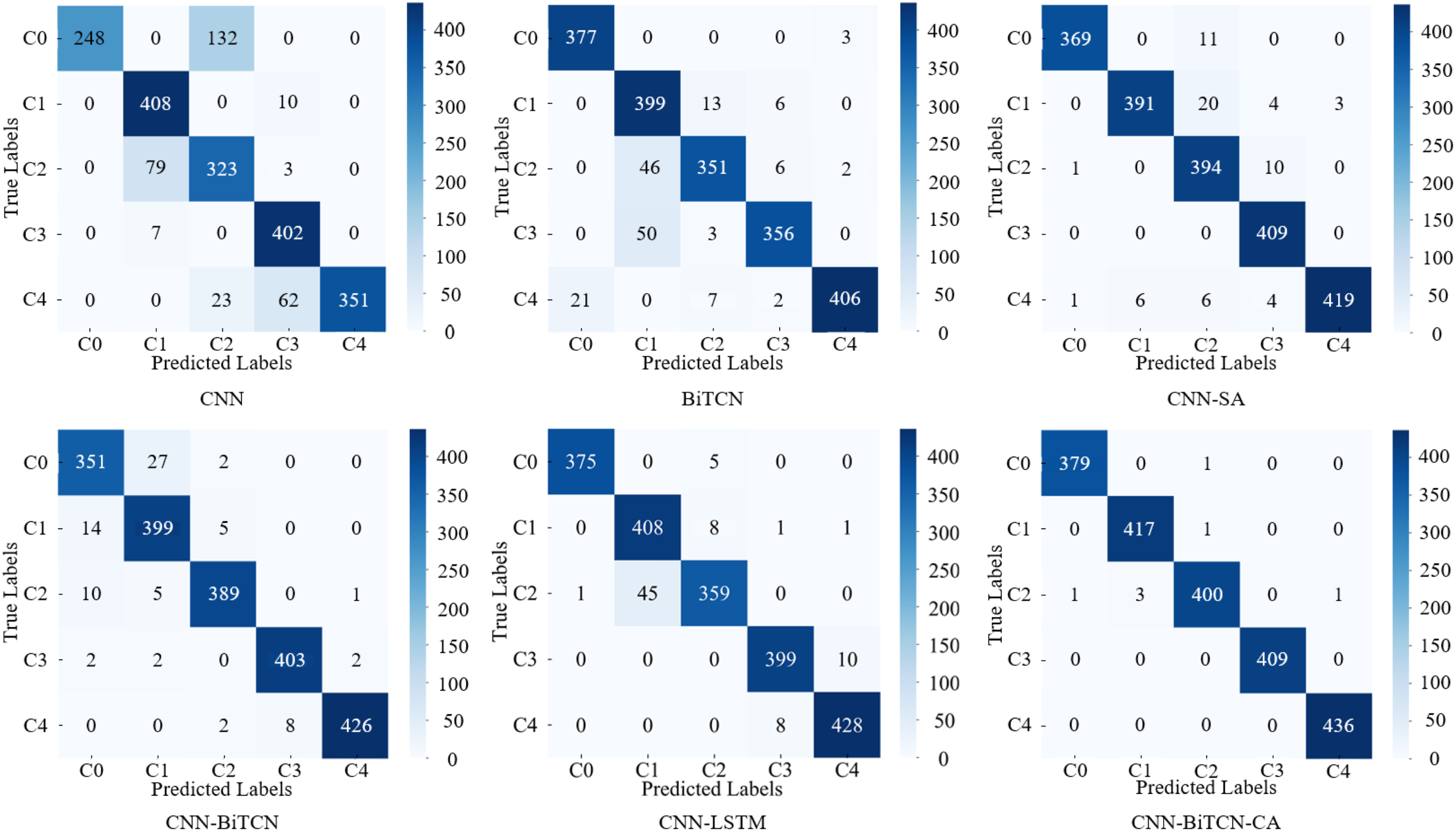
The CNN-BiTCN-CA model successfully classified different gear faults in simulated experiments, whereas the other five models experienced varying degrees of confusion. This demonstrates that the CNN-BiTCN-CA model can better extract fault features during the process of identifying gear fault types, achieving precise classification of fault types.
5.2. Feature clustering visualization
T-SNE reduces high-dimensional data to two dimensions for visualization. Points of different colors represent distinct sample categories, which correspond to the labels in the simulated dataset. Greater separation between clusters of different colors and tighter clustering of points with the same color indicate a stronger ability of the diagnostic model to discriminate between different fault features (Cai and Ma, 2022). To validate the feature extraction performance of the proposed CNN-BiTCN-CA model for gear fault diagnosis, the simulated experimental dataset was utilized, and t-SNE was employed to perform a visualization and clustering analysis of the fault features output by different diagnostic models. The results are shown in Figure 14. Visualization results of the t-SNE features for the different diagnostic models.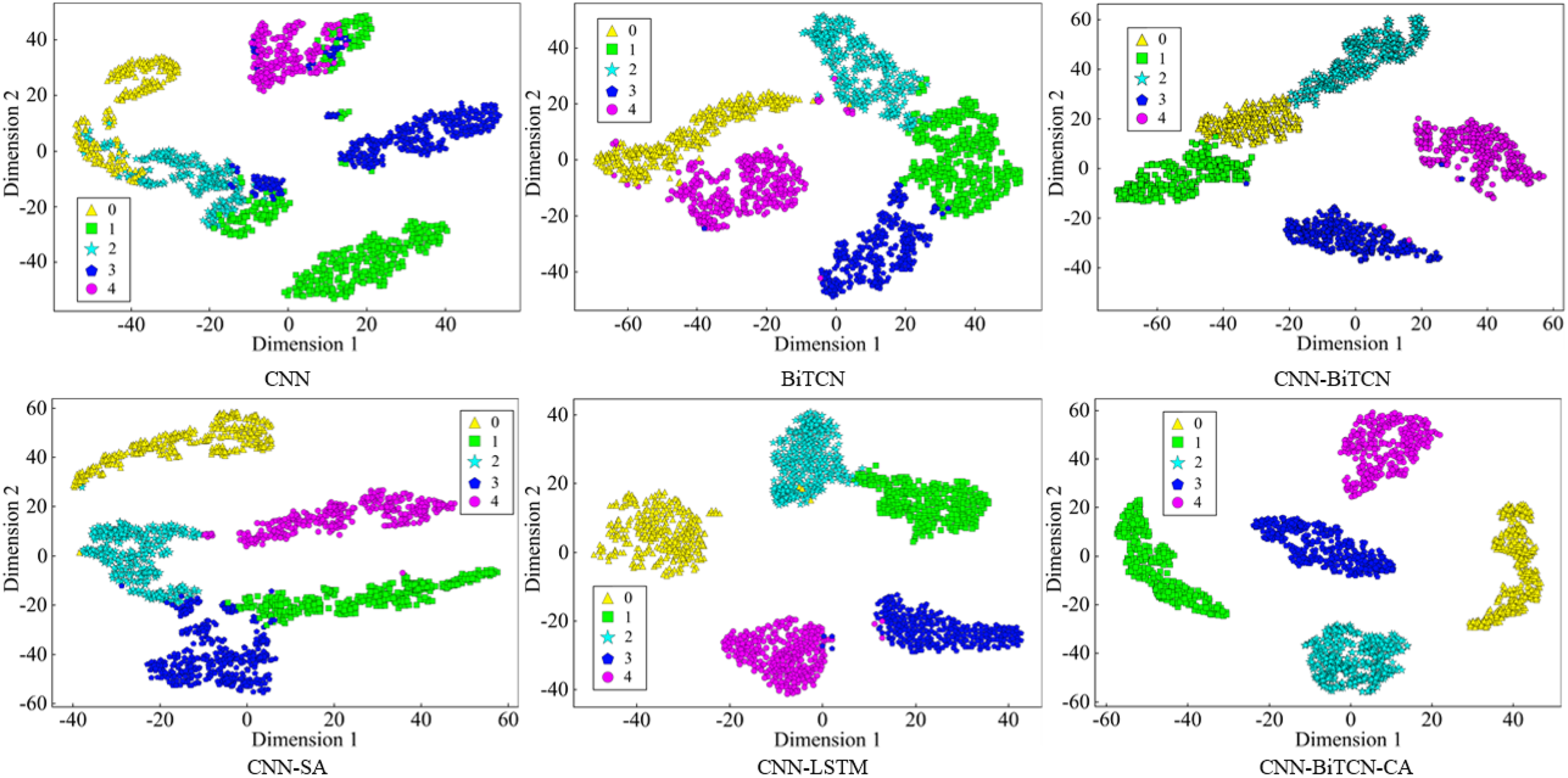
Figure 14 illustrates that when using the CNN model for diagnosis, except for Label 3, the other four categories of labels exhibit varying degrees of feature confusion. When using the BiTCN model for diagnosis, all five categories of labels display boundary ambiguity and feature confusion. Furthermore, when employing the CNN-BiTCN model for diagnosis, the feature boundaries among Label 0, Label 1, and Label 2 exhibit ambiguity. Similarly, with the CNN-LSTM model, the visualized feature boundaries of Label 1 and Label 2 are indistinct, accompanied by partial feature confusion. When using the CNN-SA model for diagnosis, apart from Label 0, the remaining four categories of labels also exhibit feature confusion. This indicates that the CNN, BiTCN, and CNN-SA diagnostic models are unable to accurately identify the location of faults. In contrast, when employing the CNN-BiTCN-CA model for feature extraction, the feature clustering boundaries are clear and free from confusion, enabling precise identification of different fault types.
The feature clustering results demonstrate that the gear fault diagnosis method, incorporating a feature cross-attention mechanism, enhances intra-class feature aggregation, reduces inter-class feature overlap, and thereby achieves superior fault classification accuracy.
5.3. Experimental dataset validation from the Southeast University
Based on the SUFD dataset, training and testing analysis were conducted using the approach introduced above under identical conditions. The training accuracy of the CNN-BiTCN-CA model on the SUFD spur gear dataset achieved 99.85%, and the confusion matrix along with the clustering analysis results are presented in Figure 15. Supplementary experimental feature visualization and confusion matrix.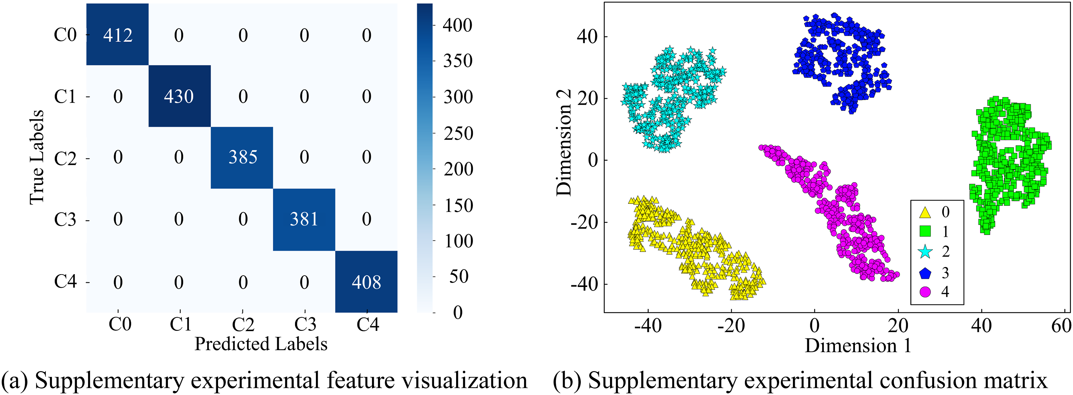
As shown in Figure 15, the classification results from the CNN-BiTCN-CA model show no signs of confusion in the confusion matrix. The feature clustering results demonstrate clear boundaries with no evidence of feature confusion. These results collectively validate the robust accuracy of the CNN -BiTCN-CA model in diagnosing gear failure types.
6. Conclusion
This paper develops a gear fault diagnosis method based on a feature cross-attention mechanism to enhance the accuracy of feature extraction and fault classification from gear vibration signals. The proposed CNN-BiTCN-CA model is constructed and evaluated experimentally. The principal findings are summarized as follows: (1) Through time-frequency reconstruction of the raw signal and feature fusion based on a cross-attention mechanism, the issue of incomplete fault feature extraction has been resolved, thereby improving the accuracy of fault classification. (2) A gearbox fault simulation test bench was established to collect vibration signals under normal conditions and four fault types. Subsequently, a fault dataset was constructed using the sliding window method. (3) Under a Gaussian white noise environment with a SNR of 7.08 dB, the CNN-BiTCN-CA model achieved a gear fault diagnosis accuracy of approximately 99.85%, which represents an improvement of approximately 14.61%, 7.58%, 3.77%, 3.60%, and 2.74% compared to CNN, BiTCN, CNN-BiTCN, CNN-SA, and CNN-LSTM, respectively. Under Gaussian white noise with a signal-to-noise ratio (SNR) of 1.77 dB, the proposed model maintained a diagnostic accuracy of 95.82%. On the SUFD gearbox fault dataset, the proposed method achieved a diagnostic accuracy of 99.55%. These results demonstrate that the CNN-BiTCN-CA model exhibits excellent diagnostic performance and robustness. Furthermore, the clustering analysis of the extracted fault features validates the model’s effectiveness for gear fault classification.
Footnotes
Funding
The authors disclosed receipt of the following financial support for the research, authorship, and/or publication of this article: This research was supported by the National Natural Science Foundation of China (52204169), Liaoning Province Natural Science Foundation Joint Funding Program Projects (20240301, 20240326, 20240318), and Scientific Research Project of Liaoning Provincial Education Department (LJ212510147029, JYTMS20230063).
Declaration of conflicting interests
The authors declare that they have no known competing financial interests or personal relationships that could have appeared to influence the work reported in this paper.
Data Availability Statement
The data sets generated during and/or analyzed during the current study are available from the corresponding author upon reasonable request.