Dual-time variable dual-pulse intermittent control strategy of a novel six-dimensional memristive hyper-chaotic system

Abstract

This paper constructs a novel six-dimensional hyper-chaotic system by incorporating a flux-controlled memristor as a nonlinear feedback element into an existing five-dimensional chaotic system. The dynamical characteristics of the proposed system are systematically investigated by means of Lyapunov exponent spectra, Kaplan–Yorke dimension calculation, bifurcation diagrams, Poincaré maps, and power spectral analysis, showing that the system exhibits rich parameter-dependent behaviors. Its physical implementability is validated via analog circuit simulation. To stabilize the resulting hyper-chaotic dynamics, a dual-time variable dual-pulse intermittent control strategy is proposed, in which the widths of the controlled and uncontrolled phases decrease monotonically with a fixed step size, while the two impulsive gains decay exponentially. Sufficient conditions for exponential stability are derived via Lyapunov theory and formulated as linear matrix inequalities feasibility problems. Numerical simulations show that the proposed controller can rapidly stabilize both the newly constructed six-dimensional memristive hyper-chaotic system and a four-dimensional hyper-chaotic financial system, demonstrating broad applicability to nonlinear dynamical models arising in engineering and economics.

Keywords

hyper-chaotic system memristor intermittent control Lyapunov stability linear matrix inequality

1. Introduction

The study of nonlinear dynamical systems was fundamentally transformed by the landmark work of Lorenz (Lorenz, 1963), whose discovery of deterministic chaos in atmospheric convection demonstrated that even purely deterministic systems can produce behavior of irreducible unpredictability. Since that seminal contribution, chaos theory has permeated a broad spectrum of scientific and engineering disciplines, providing a unified conceptual framework for understanding systems whose dynamics are governed by sensitive dependence on initial conditions (Frederickson et al., 1983; Wolf et al., 1985). The butterfly effect—whereby arbitrarily small perturbations to initial states are amplified exponentially over time—is one of the most recognizable signatures of chaotic behavior. Paradoxically, this same unpredictability has been harnessed constructively: in secure communication, the aperiodic and broadband nature of chaotic signals renders them natural carriers for information concealment (Abou El Qassime et al., 2025; Ulutas, 2025), and their complex statistical properties underpin a rapidly growing body of work on chaos-based image encryption and pseudorandom number generation (Abba et al., 2024; Kopp and Samuilik, 2025; Wang et al., 2024). Recent studies have further emphasized the optimization of chaotic maps for image-encryption applications. For example, Ding et al. (2026a) designed a three-dimensional logistic map for image encryption, while Ding et al. (2026b) proposed a sine-based reconstruction approach to improve the dynamical performance of two-dimensional chaotic maps. Gao et al. (2025b) further extended this line of research by developing a video-segment encryption framework based on a discrete sinusoidal memristive Rulkov neuron.

Hyper-chaotic systems, distinguished from ordinary chaotic systems by possessing at least two simultaneously positive Lyapunov exponents, have emerged as a particularly active frontier of nonlinear dynamics research. The coexistence of instability across multiple independent phase-space directions endows hyper-chaotic attractors with a richer geometric structure, a higher Kaplan–Yorke dimension, and greater resistance to reconstruction attacks compared with their lower-dimensional counterparts (Mobayen et al., 2024; Yan et al., 2025). These properties make hyper-chaotic systems strongly preferred for cryptographic and secure communication applications where adversarial reconstruction must be thwarted (Rong et al., 2024; Zhang et al., 2025). Constructing new hyper-chaotic systems of increasing dimensionality and dynamic complexity therefore remains an important ongoing research objective.

Memristors, first proposed theoretically by Chua (Chua, 1971) as the fourth fundamental passive circuit element and physically realized by Strukov et al. (Strukov et al., 2008), have emerged as pivotal building blocks in the construction of high-dimensional hyper-chaotic systems. The defining feature of a memristor—that its instantaneous resistance is a nonlinear function of the cumulative charge that has passed through it—confers upon any circuit in which it is embedded a memory-dependent nonlinearity unavailable from conventional passive elements. When introduced as a feedback element into existing chaotic systems, flux-controlled memristors can dramatically elevate the dimensionality and attractor complexity of the resulting dynamics (Jie et al., 2025; Yang et al., 2025). The design and hardware validation of such memristive systems have attracted considerable attention: Gokyildirim et al. (2024) demonstrated fractional-order sliding mode control of a four-dimensional memristive chaotic system with circuit-level verification, while Yesil et al. (2025) introduced a compact seven-term memristive jerk circuit and validated both its nonlinear dynamics and microcontroller-based stabilization. Recent studies have more broadly confirmed the applicability of memristive hyper-chaotic systems to circuit implementation, control design, and selected engineering applications, with numerical simulations often corroborated by analog circuit experiments (Li et al., 2023; Mobayen et al., 2024; Zhu et al., 2025). Recent work has also broadened the hardware and application scope of memristive circuits. Gao et al. (2025a) designed a three-dimensional memristive cubic map with dual discrete memristors and demonstrated its implementation and application in image encryption. In addition, Gao et al., 2026b, 2026a further explored memristor-based neural and decision-making circuits exhibiting classical conditioning, fear generalization, and adaptive control capability. While the memristive hyper-chaotic landscape has been substantially enriched by these contributions, existing work has largely centered on systems of three to five state dimensions; the systematic construction of six-dimensional memristive hyper-chaotic systems from five-dimensional chaotic predecessors, together with rigorous characterization of their bifurcation structure and circuit feasibility, has received comparatively little attention and constitutes a natural extension of the current research frontier.

Effective stabilization of hyper-chaotic systems constitutes a fundamental challenge in nonlinear control theory, and the past decade has witnessed the development of a diverse arsenal of control strategies. Adaptive control (Ozpolat and Gulten, 2024) is well suited to systems with uncertain or time-varying parameters, dynamically adjusting the control law online; however, its performance degrades substantially when parametric drift is rapid or significant unmodeled dynamics are present. Sliding mode control (Yan et al., 2025; Zheng et al., 2024) is renowned for strong robustness against matched disturbances and the ability to enforce finite-time convergence to a user-specified sliding surface. In the memristive-chaos literature, sliding-mode-based synchronization has recently been extended to finite-time, fixed-time, and predefined-time frameworks. Lai and Wang (2024) developed finite- and fixed-time synchronization laws for memristive chaotic systems based on sliding mode reaching laws, while Lai et al. (Lai et al., 2025b; Lai and Wang, 2026) further investigated predefined-time synchronization for simple memristive chaotic systems and cyclic memristive neural networks, respectively. Related progress has also been reported for grid multiscroll memristive Chua’s circuits with predefined-time synchronization for secure communication (Lai et al., 2025a). Tan and Feng (2025) also proposed a predefined-time smooth mode control strategy with an exponential-function-based sliding surface for chaotic synchronization, further enriching the design of fast synchronization controllers for memristive nonlinear systems. More recent advances have further extended this paradigm to fast fixed-time formulations applied to memristor-based oscillators (Mirzaei et al., 2023) and predefined-time stabilization frameworks with event-triggered mechanisms for chaotic systems (Zhang and Zang, 2025); nevertheless, the chattering phenomenon inherent in discontinuous switching can excite unmodeled high-frequency dynamics and cause actuator wear in practical implementations. Beyond conventional model-based strategies, learning-based optimal control has also emerged as a promising alternative for nonlinear systems. For instance, Song and Tong (2025) developed an inverse reinforcement learning optimal control framework for Takagi–Sugeno fuzzy systems, showing that data-driven optimal control can effectively handle complex nonlinear dynamics without requiring a predefined cost function. Impulsive control, in which instantaneous state resets are applied at discrete time instants, achieves fast stabilization through sparse intervention. For example, Xie et al. (2022) proposed a three-stage-impulse control strategy for a memristor-based Chen hyper-chaotic system, demonstrating that properly designed impulsive actions can effectively stabilize complex nonlinear dynamics. This class of methods has also been rigorously extended to event-triggered formulations that reduce actuation frequency while preserving Lyapunov stability guarantees (Li et al., 2020; Li and Wang, 2025; Tu et al., 2025); however, the conventional fixed impulse period renders such schemes insensitive to the time-varying divergence intensity of the chaotic trajectory. More critically, Liu et al. (2020) established exponential input-to-state stability for aperiodically intermittent control schemes via Lyapunov methods—a foundational result that motivates designs with variable timing structures. Intermittent control, a natural complement to impulsive control, applies continuous feedback only within designated active sub-intervals of each period and has been shown effective for both stabilization and synchronization of memristive hyper-chaotic systems (Chen, 2025; Li et al., 2023; Liu and Ye, 2020). Recently, Ni et al. (2026) further extended intermittent frameworks to switched neutral networked systems, and Yue et al. (2026) proposed universal intermittent state-constrained control for general nonlinear systems, underscoring that variable-structure intermittent strategies are a vibrant current frontier. More recently, Tang et al. (2025) achieved finite-time synchronization of coupled fractional-order systems via intermittent IT-2 fuzzy control, further broadening the applicability of intermittent strategies to fractional-order nonlinear dynamics. Nevertheless, a fundamental limitation shared by most existing intermittent and impulsive schemes is the use of fixed control widths and fixed inter-impulse spacings. Such rigidity prevents the controller from adapting to the evolving state trajectory: the fixed-width structure applies identical control effort regardless of whether the system is in a highly divergent phase or approaching the equilibrium, which can result in either wasted energy or insufficient suppression.

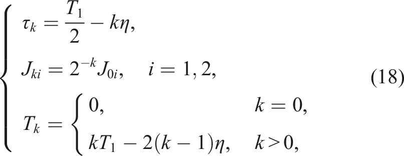
The control strategy proposed in this paper employs a piecewise structure. Figure 1 shows a detailed schematic diagram of the control process, in which the arrows indicate the direction in which the control bandwidth varies with the iterative bandwidth. In the first stage, continuous control with an intensity of K is applied. At the end of this stage, a pulse control with an intensity of J_k1 is applied. The second stage involves no control, but a pulse control with an intensity of J_k2 is applied at its conclusion. The control bandwidth of both stages decreases monotonically as the control period k increases, while the pulse intensity at the end of both stages decays exponentially as the control period k increases. In which, η denotes the step size of the control width sequence, and σ denotes the threshold, which is a positive number close to zero. When the width of the two phases exceeds this threshold, the width is no longer altered. This ensures that control is applied consistently throughout the iteration and maintains the continuity of the control process. Compared with traditional control methods, this control strategy offers faster response times and greater robustness, making it widely applicable to most existing nonlinear systems. Furthermore, this paper applies the proposed method to the control of newly developed hyper-chaotic systems and four-dimensional hyper-chaotic financial systems, and verifies the effectiveness of the method through numerical simulations.

Figure 1.

The control schematic diagram of dual-time variable dual-pulse intermittent control strategy.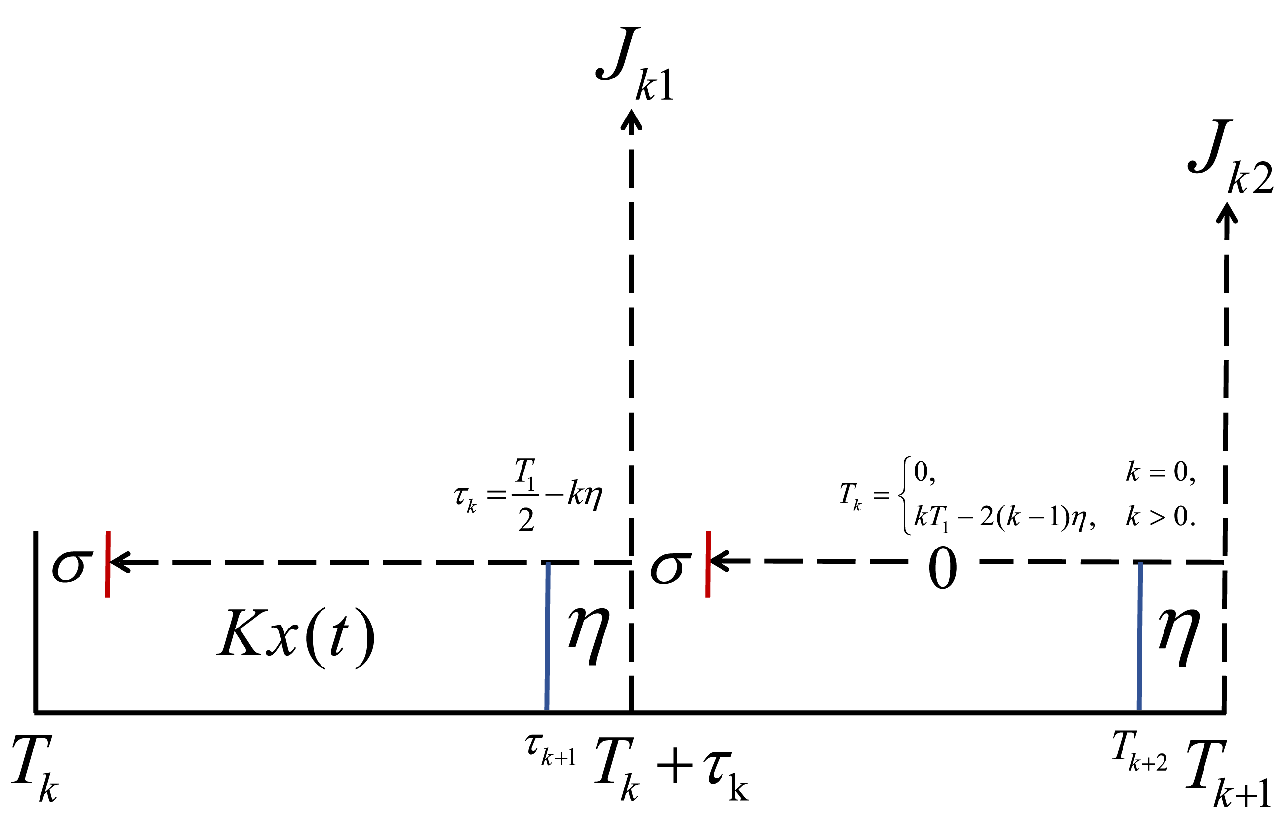

Considering all the discussed scenarios, the primary findings and innovations presented in this study can be encapsulated in the following points.

(i) A novel six-dimensional memristive hyper-chaotic system is constructed by incorporating a flux-controlled memristor as a nonlinear feedback element into a five-dimensional chaotic system, which enhances the system’s dynamic complexity. An equivalent analog circuit is designed to ensure the consistency between theoretical analysis and practical implementation;

(ii) A new dual-time variable dual-pulse intermittent control strategy is proposed to overcome the limitation of fixed control width in traditional schemes, which often fail to meet practical control requirements. A key feature of this strategy is that the control bandwidth in both stages varies cyclically and monotonically by a fixed step size η, while the amplitudes of the two independent pulse gains, J_k1 and J_k2, decay exponentially as the control period k increases. This framework allows flexible adjustment of the control intensity, making it more suitable for both hyper-chaotic systems and practical control applications;

(iii) This paper establishes a mathematical model of a nonlinear system and generalizes the proposed control strategy to general nonlinear equations. The control strategy has been successfully applied to stabilize both the newly constructed six-dimensional memristive hyper-chaotic system and the four-dimensional hyper-chaotic financial system, demonstrating its broad applicability to both engineering and economic nonlinear dynamical models.

The structure of the paper is as follows: Section 2 introduces the six-dimensional hyper-chaotic system with flux-controlled memristor feedback and presents its mathematical equations. Section 3 analyzes the dynamic behavior of the newly proposed system. Section 4 provides an overview of general nonlinear systems, controller design, and the underlying mathematical principles. Section 5 presents a new dual-time variable dual-pulse intermittent control strategy and derives conditions for exponential stability. Section 6 demonstrates the effectiveness of the proposed control strategy through numerical simulations. Finally, Section 7 concludes the paper.

2. Description of the proposed six-dimensional hyper-chaotic system

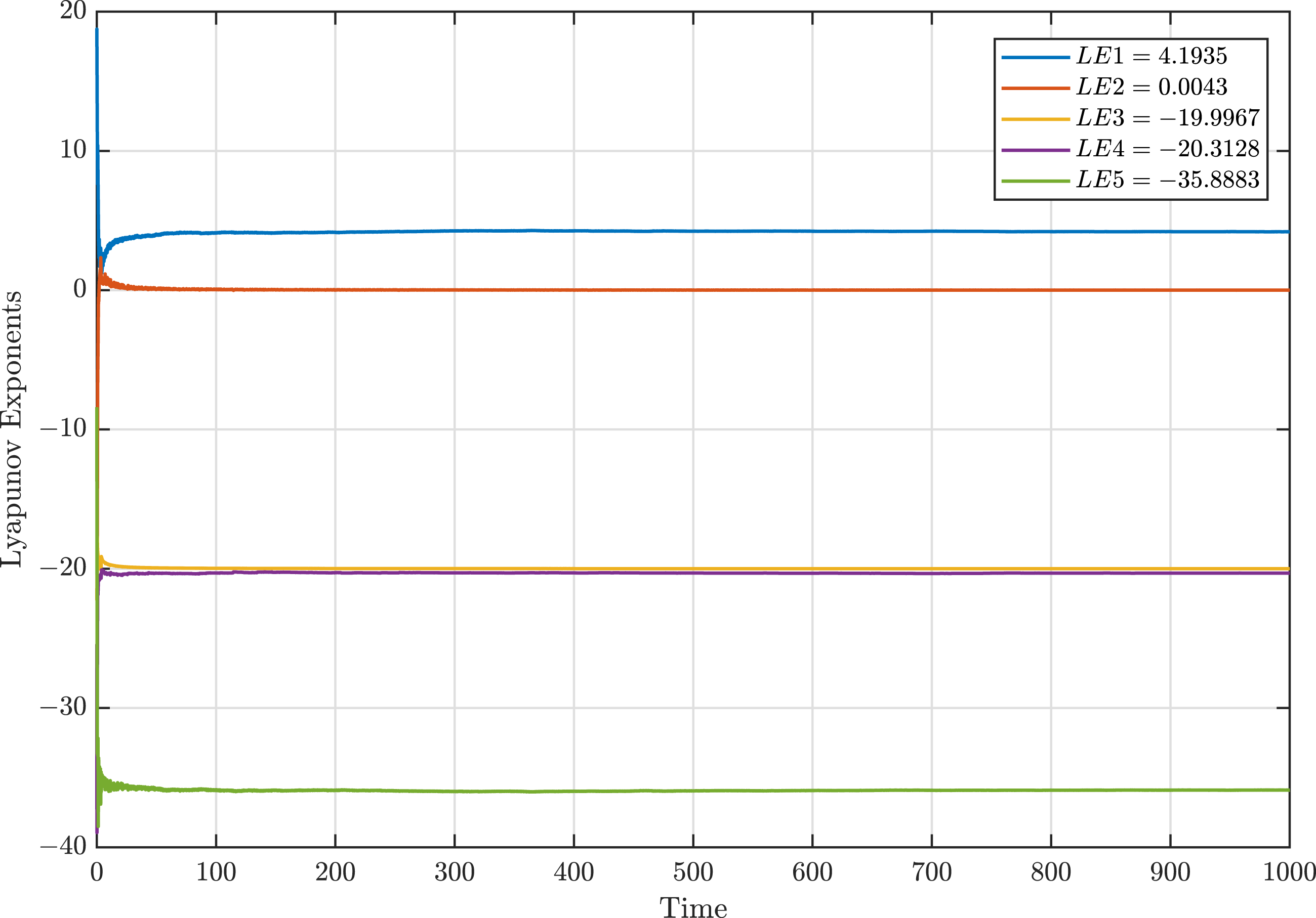
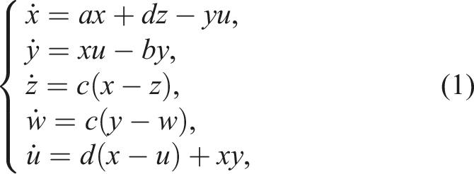
The five-dimensional chaotic system (Zhang and Wang, 2025) is described by the following set of differential equations

\{\begin{cases} \dot{x} = a x + d z - y u, \\ \dot{y} = x u - b y, \\ \dot{z} = c (x - z), \\ \dot{w} = c (y - w), \\ \dot{u} = d (x - u) + x y, \end{cases}

(1)

where a, b, c, and d represent the real system parameters, x, y, z, w, and u are system state variables. When the system’s parameters are set as a = 16, b = 40, c = 20, d = 8, and the initial conditions are assigned as [0.1,0.1,0.1,0.1,0.1]^T, system (1) exhibits highly intricate chaotic attractors, as depicted in Figure 2. Figure 3 displays the five Lyapunov exponents of the system, where one exponent is positive, one is zero, and the sum of the five exponents is less than zero. Consequently, the system is chaotic.

Figure 2.

Phase portraits of the five-dimensional chaotic system in different planes. (a) x-w plane. (b) y-w plane.

Figure 3.

The Lyapunov exponent distribution of the five-dimensional chaotic system.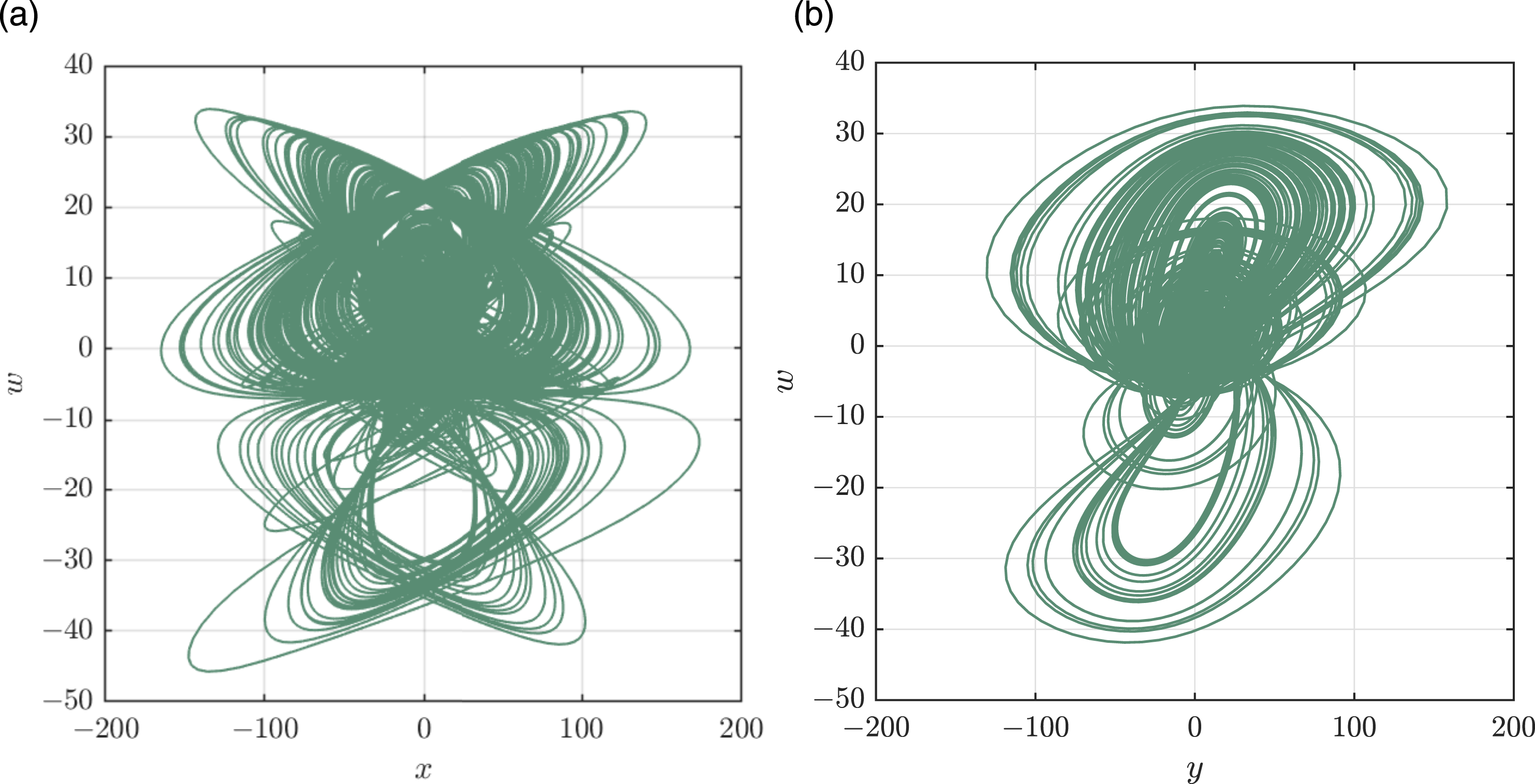

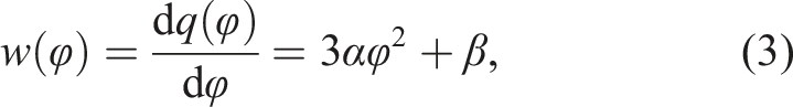
Memristors establish a link between magnetic flux φ and charge q, and are categorized into flux-controlled and charge-controlled types. Their nonlinear characteristics significantly enhance the dynamic complexity of chaotic systems. In this study, a flux-controlled memristor with nonlinear state feedback is added to the five-dimensional system, resulting in the development of a new hyper-chaotic system. The relationship between charge and flux in the flux-controlled memristor is expressed as follows

q (φ) = α φ^{3} + β φ,

(2)

where q denotes the charge passing through the flux-controlled memristor and α and β are non-negative constants. The slope of the curve, which represents the charge changes in relation to the magnetic flux, is termed memductance w(φ). Its mathematical formulation is as follows

w (φ) = \frac{d q (φ)}{d φ} = 3 α φ^{2} + β,

(3)

the I - V (current i(t) - voltage u(t)) characteristics of the flux-controlled memristor are described as follows

\begin{aligned} i (t) & = w (φ) u (t), \\ u (t) & = \frac{d φ}{d t} . \end{aligned}

(4)

To verify the memory characteristics of the proposed model, we investigate the response of the hysteresis loop area to an external sinusoidal voltage excitation defined as u(t) = A sin (2πft), with model parameters set to α = 0.01, and β = 0.01. Figure 4 illustrates the volt—ampere characteristic curves of the flux-controlled memristor under excitations with different frequencies and amplitudes. Specifically, Figure 4(a) presents the response at a fixed voltage amplitude of A = 20 V for frequencies f = 5 Hz, 10 Hz, and 15 Hz, while Figure 4(b) depicts the response at a fixed frequency of f = 5 Hz for voltage amplitudes A = 10 V, 15 V, and 20V. All resulting curves exhibit pinched hysteresis loops resembling a tilted figure-eight shape confined to the first and third quadrants. The lobe area of the hysteresis loop is negatively correlated with the frequency f and positively correlated with the amplitude A, demonstrating a clear dependence on the excitation signal. These frequency and amplitude-dependent behaviors confirm that the proposed model satisfies the fundamental fingerprints of a memristor and therefore provides a reasonable basis for the subsequent memristive hyper-chaotic system construction.

Figure 4.

Volt - Ampere characteristic curves of the flux-controlled memristor. (a) Hysteresis loops under different excitation frequencies. (b) Hysteresis loops under different voltage amplitudes.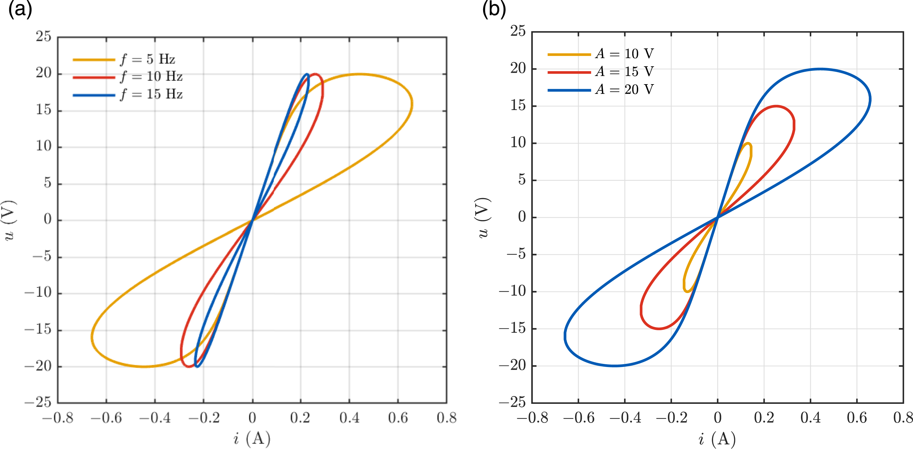

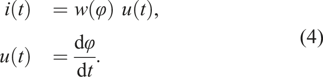
If we let the voltage u across the flux-controlled memristor be represented as x and the magnetic flux as v, the following expression is obtained

i (t) = w (φ) u (t) = (3 α v^{2} + β) x .

(5)

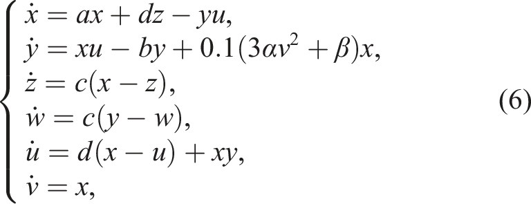
By adding a new variable w as a driving force to the five-dimensional system and using memristor-based feedback, a six-dimensional hyper-chaotic system is constructed. The resulting hyper-chaotic system is mathematically described by nonlinear ordinary differential equations as follows

\{\begin{cases} \dot{x} = a x + d z - y u, \\ \dot{y} = x u - b y + 0.1 (3 α v^{2} + β) x, \\ \dot{z} = c (x - z), \\ \dot{w} = c (y - w), \\ \dot{u} = d (x - u) + x y, \\ \dot{v} = x, \end{cases}

(6)

in this system, [x,y,z,w,u,v]^T ∈ R⁶ denotes the state vector, with a, b, c, d, α, and β as positive constant parameters.

3. Dynamic analysis of the proposed six-dimensional hyper-chaotic system

3.1. Phase diagrams and Lyapunov exponent distribution

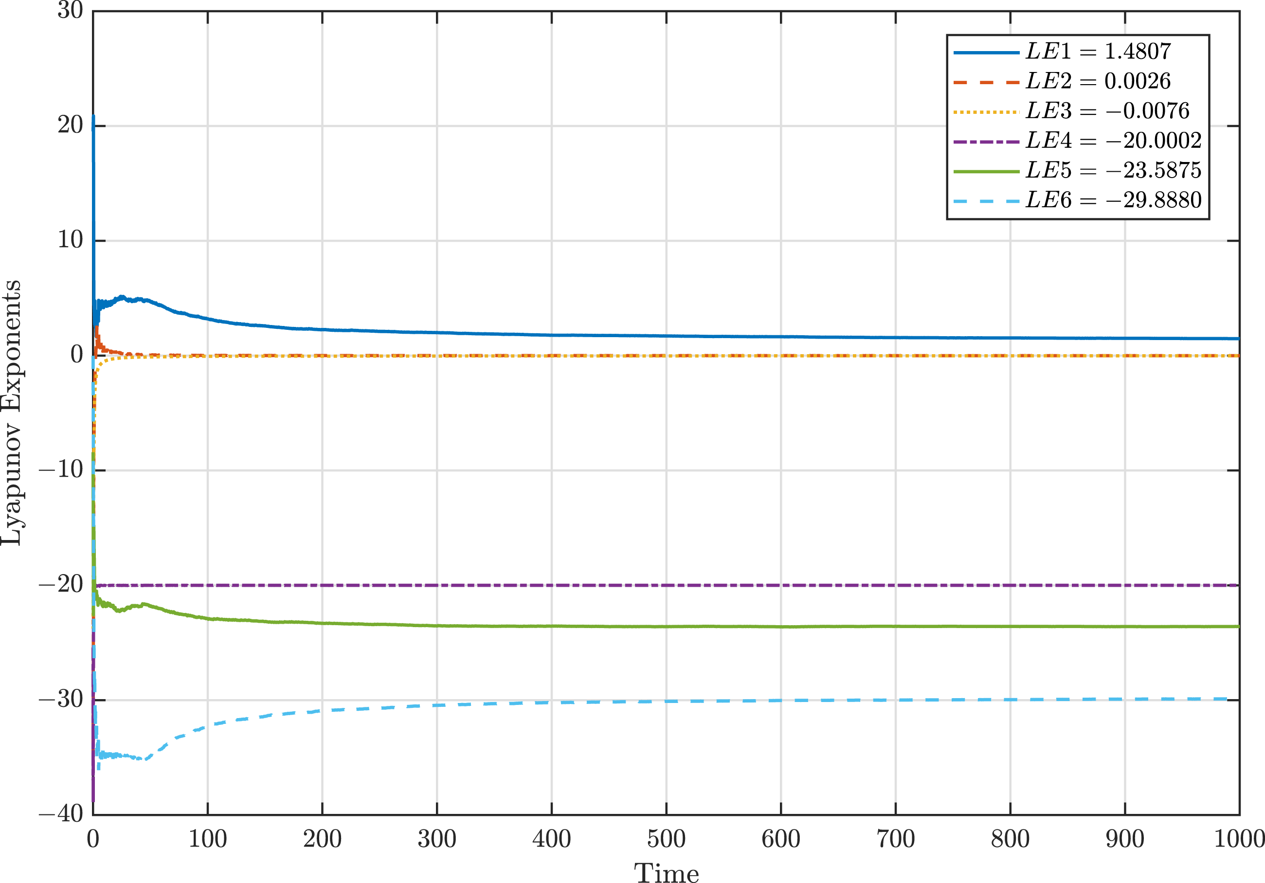
To achieve complex chaotic dynamical behavior in system (6), we set the system parameters a = 16, b = 40, c = 20, d = 8, α = 0.01, and β = 2. The initial conditions of the system are given by [0.1,0.1,0.1,0.1,0.1,0.1]^T. With the chosen parameters, the system exhibits intricate hyper-chaotic dynamics. The corresponding attractor phase diagram is displayed in Figure 5. Using the Wolf method (Wolf et al., 1985) to calculate the Lyapunov exponents for the system’s state variables, Figure 6 displays the six Lyapunov exponents of the system, where two exponents are positive, and the sum of the six exponents is less than zero. Consequently, the system is hyper-chaotic.

Figure 5.

Phase portraits of the six-dimensional hyper-chaotic system in different planes. (a) x-z plane. (b) y-z plane.

Figure 6.

The Lyapunov exponent distribution of the six-dimensional hyper-chaotic system.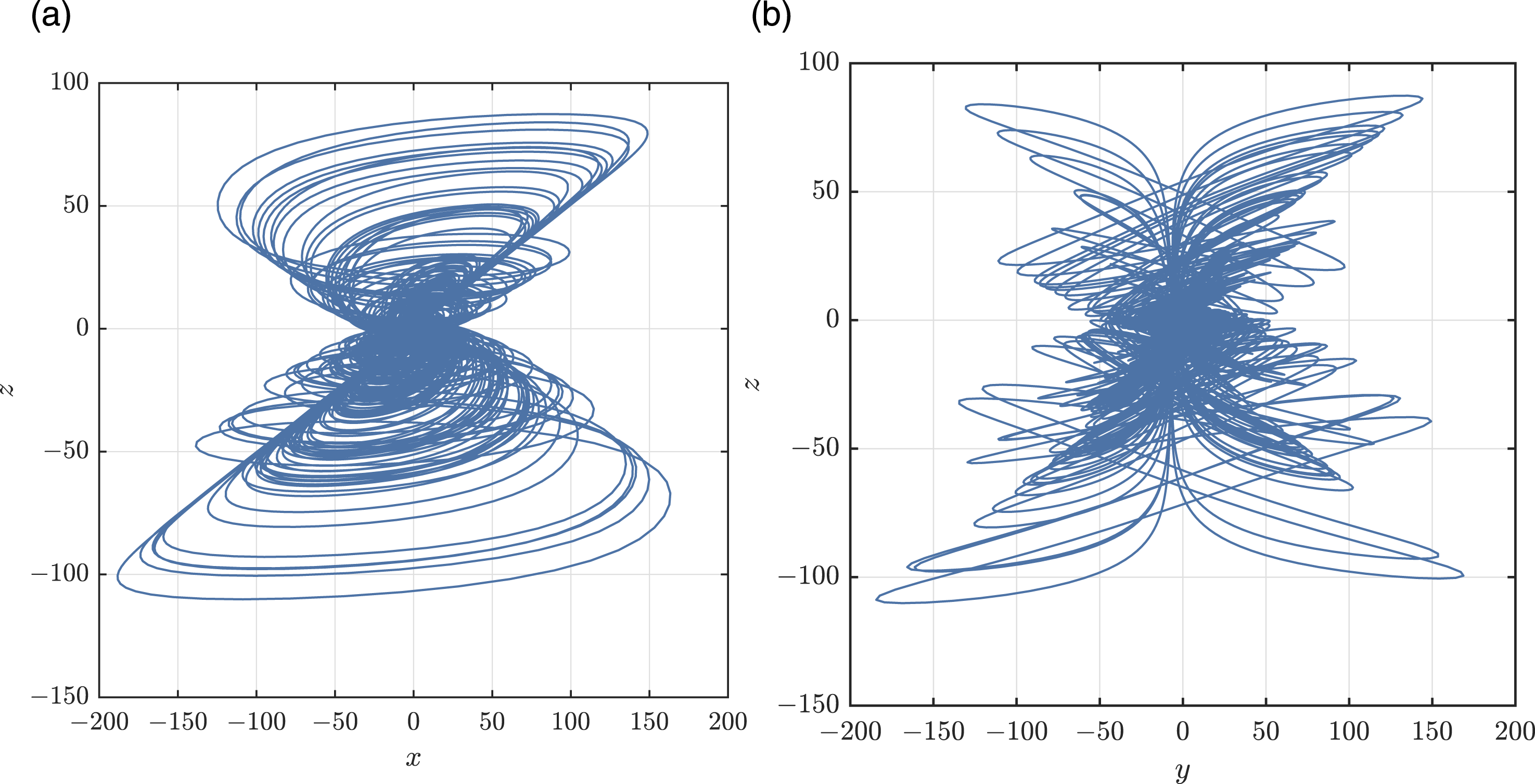

The Lyapunov dimension D_KY (Frederickson et al., 1983) of the attractor is calculated as

D_{K Y} = j + \frac{\sum_{i = 1}^{j} L E i}{| L E (j + 1) |},

(7)

where j is the largest integer such that

\sum_{i = 1}^{j} L E i > 0

and

\sum_{i = 1}^{j + 1} L E i < 0

. Substituting the computed Lyapunov exponents yields

D_{K Y} = 3 + \frac{1.4807 + 0.0026 - 0.0076}{20.0002} \approx 3.0738 .

(8)

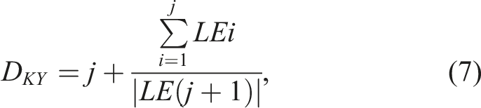
The fractal dimension quantitatively characterizes the spatial filling capacity and structural complexity of chaotic attractors within phase space. Its non-integer nature reflects the attractor’s self-similar fractal structure. For hyper-chaotic attractors, the fractal dimension typically exceeds 3, indicating that trajectories diverge and fold simultaneously in multiple directions, forming complex geometric structures of higher dimensions.

3.2. The dissipative property

System (6) exhibits dissipative behavior, and its dissipativity ∇V can be derived from the following expression

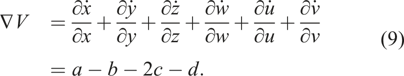
\begin{aligned} \nabla V & = \frac{\partial \dot{x}}{\partial x} + \frac{\partial \dot{y}}{\partial y} + \frac{\partial \dot{z}}{\partial z} + \frac{\partial \dot{w}}{\partial w} + \frac{\partial \dot{u}}{\partial u} + \frac{\partial \dot{v}}{\partial v} \\ = a - b - 2 c - d . \end{aligned}

(9)

By substituting the parameter values a = 16, b = 40, c = 20, and d = 8, we find ∇V = −72 < 0. This indicates that the system exhibits dissipative behavior and exponential convergence properties, converging exponentially at a rate of e⁻⁷². As time approaches infinity, all trajectories will ultimately be confined within a zero-volume symmetric subset, leading the phase diagram to approach a chaotic attractor.

3.3. Equilibrium points and stability

Identifying and examining the equilibrium positions within chaotic systems is essential for assessing their stability. By equating the left-hand side of system (6) to zero, we can obtain

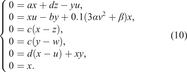
\{\begin{cases} 0 = a x + d z - y u, \\ 0 = x u - b y + 0.1 (3 α v^{2} + β) x, \\ 0 = c (x - z), \\ 0 = c (y - w), \\ 0 = d (x - u) + x y, \\ 0 = x . \end{cases}

(10)

Therefore, the equilibrium set of the system is

S = {x = 0, y = 0, z = 0, w = 0, u = 0, v = k ∣ k \in R},

(11)

where

k \in R

is any real number, implying that the system possesses an infinite number of equilibrium points. If we linearize the system at these equilibrium points, the system’s Jacobian matrix is given by. To examine the stability of the hyper-chaotic system at these points, we linearize the system at the equilibrium points and compute its Jacobian matrix. The Jacobian matrix at the equilibrium point S in system (6) is

J = [\begin{matrix} a & 0 & d & 0 & 0 & 0 \\ 0.1 (3 α k^{2} + β) & - b & 0 & 0 & 0 & 0 \\ c & 0 & - c & 0 & 0 & 0 \\ 0 & c & 0 & - c & 0 & 0 \\ d & 0 & 0 & 0 & - d & 0 \\ 1 & 0 & 0 & 0 & 0 & 0 \end{matrix}] .

(12)

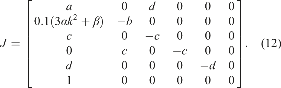
Therefore, the eigenvalues corresponding to these equilibrium points can be determined. The calculation of these eigenvalues is done using equation (13)

|λ I - J| = 0,

(13)

with the parameters a = 16, b = 40, c = 20, d = 8, α = 0.01, and β = 2. The eigenvalues at the equilibrium set S are given as λ₁ = 0, λ₂ = −8, λ₃ = λ₄ = −20, λ₅ = 14, and λ₆ = −40. It can be observed that there is a positive eigenvalue, accordingly, it has been established that the system’s equilibrium position exhibits instability.

3.4. Bifurcation diagram and Poincaré map analysis

System (6) exhibits an infinite number of equilibrium points, including an infinite number of unstable equilibrium points. This causes the system to display a rich variety of dynamic behaviors, such as periodic orbits, chaos, and hyper-chaos. To further investigate the effects of the system parameters on these dynamical behaviors, we compute the Lyapunov exponent spectra and bifurcation diagrams for parameter ranges of a from 0 to 20, b from 20 to 50, c from 0 to 30, d from 0 to 15, α from 0 to 10, and β from 0 to 10. These dynamic analysis methods provide detailed information regarding the stability of the system, chaotic behavior, and the influence of different parameters on the system dynamics. The initial conditions [0.1,0.1,0.1,0.1,0.1,0.1]^T are fixed.

Case 1

The system parameters are set as b = 40, c = 20, d = 8, α = 0.01, and β = 2, with a ∈ (0, 20). The corresponding Lyapunov exponent spectrum and the bifurcation diagram of the state variables are shown in Figure 7.

Figure 7.

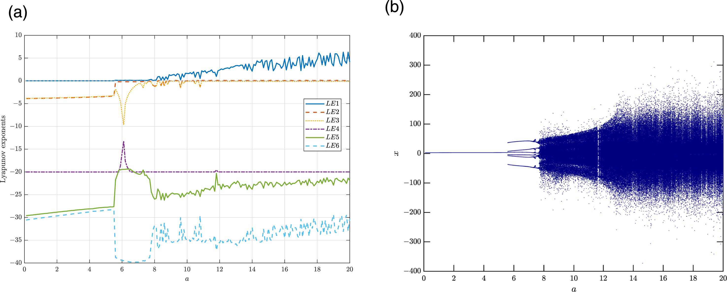
The system’s Lyapunov exponents and bifurcation diagram showing state variable x versus parameter a. (a) Lyapunov exponent spectrum. (b) Bifurcation diagram.

Upon detailed analysis, it is observed that the system exhibits stable equilibrium dynamics within the interval a ∈ (0, 5.6), as indicated by the Lyapunov exponent distribution of (0, −, −, −, −, −), and the bifurcation diagram shows that the system converges to a stable equilibrium point. In the range a ∈ (5.6, 7.7), the Lyapunov exponents are (0, 0, −, −, −, −), which suggests that the system is in a quasi-periodic motion state. For a ∈ (7.7, 8.9) ∪ (9.5, 9.9) ∪ (10.4, 10.9), the system presents a Lyapunov exponent distribution of (+,0, −, −, −, −), indicating a transition into chaotic behavior. When a ∈ (8.9, 9.5) ∪ (9.9, 10.4) ∪ (10.9, 20), the system exhibits two positive Lyapunov exponents, signifying that the system enters a hyper-chaotic state.

Case 2

The system parameters are set as a = 16, c = 20, d = 8, α = 0.01, and β = 2, with b ∈ (20, 50). The corresponding Lyapunov exponent spectrum and the bifurcation diagram of the state variables are shown in Figure 8.

Figure 8.

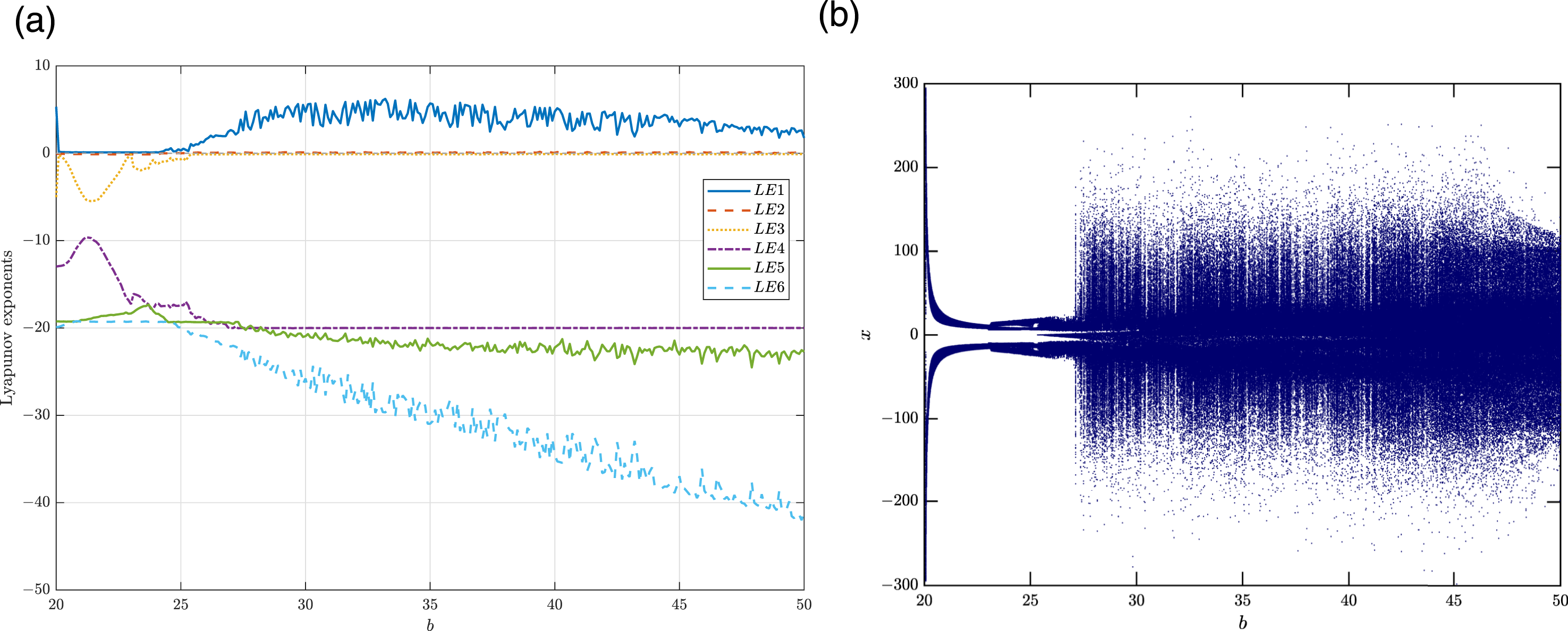
The system’s Lyapunov exponents and bifurcation diagram showing state variable x versus parameter b. (a) Lyapunov exponent spectrum. (b) Bifurcation diagram.

It is observed that, when b ∈ (20, 25.4), the system presents a Lyapunov exponent distribution of (+,0, −, −, −, −), indicating a transition into chaotic behavior. When b ∈ (25.4, 50), the system exhibits two positive Lyapunov exponents, signifying that the system enters a hyper-chaotic state.

Case 3

The system parameters are set as a = 16, b = 40, d = 8, α = 0.01, and β = 2, with c ∈ (0, 30). The corresponding Lyapunov exponent spectrum and the bifurcation diagram of the state variables are shown in Figure 9.

Figure 9.

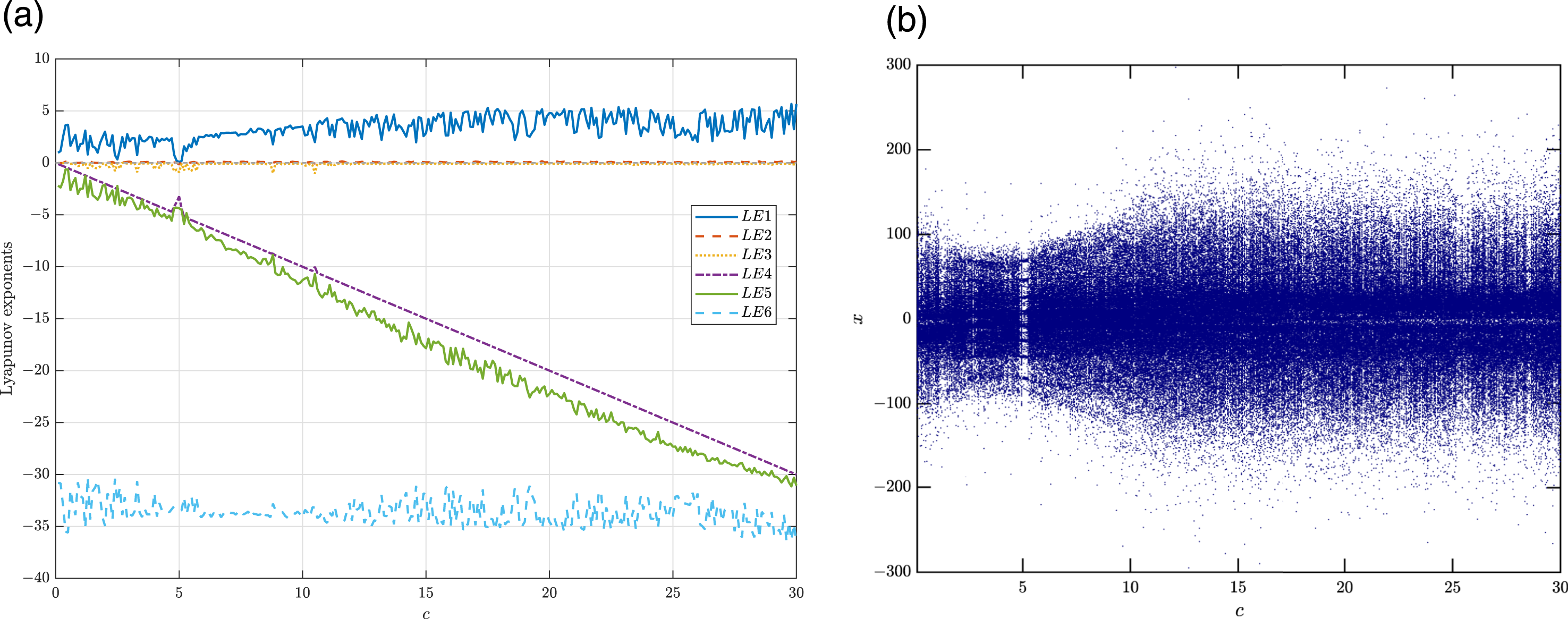
The system’s Lyapunov exponents and bifurcation diagram showing state variable x versus parameter c. (a) Lyapunov exponent spectrum. (b) Bifurcation diagram.

Upon detailed analysis, when c ∈ (2.3, 2.7) ∪ (4.7, 5.2), the Lyapunov exponents are (0, 0, −, −, −, −), which suggests that the system is in a quasi-periodic motion state. For c ∈ (0.7, 1), the system presents a Lyapunov exponent distribution of (+,0, −, −, −, −), indicating a transition into chaotic behavior. When c ∈ (0, 0.7) ∪ (1, 2.3) ∪ (2.7, 4.7) ∪ (5.2, 30), the system exhibits two positive Lyapunov exponents, signifying that the system enters a hyper-chaotic state.

Case 4

The system parameters are set as a = 16, b = 40, c = 20, α = 0.01, and β = 2, with d ∈ (0, 15). The corresponding Lyapunov exponent spectrum and the bifurcation diagram of the state variables are shown in Figure 10.

Figure 10.

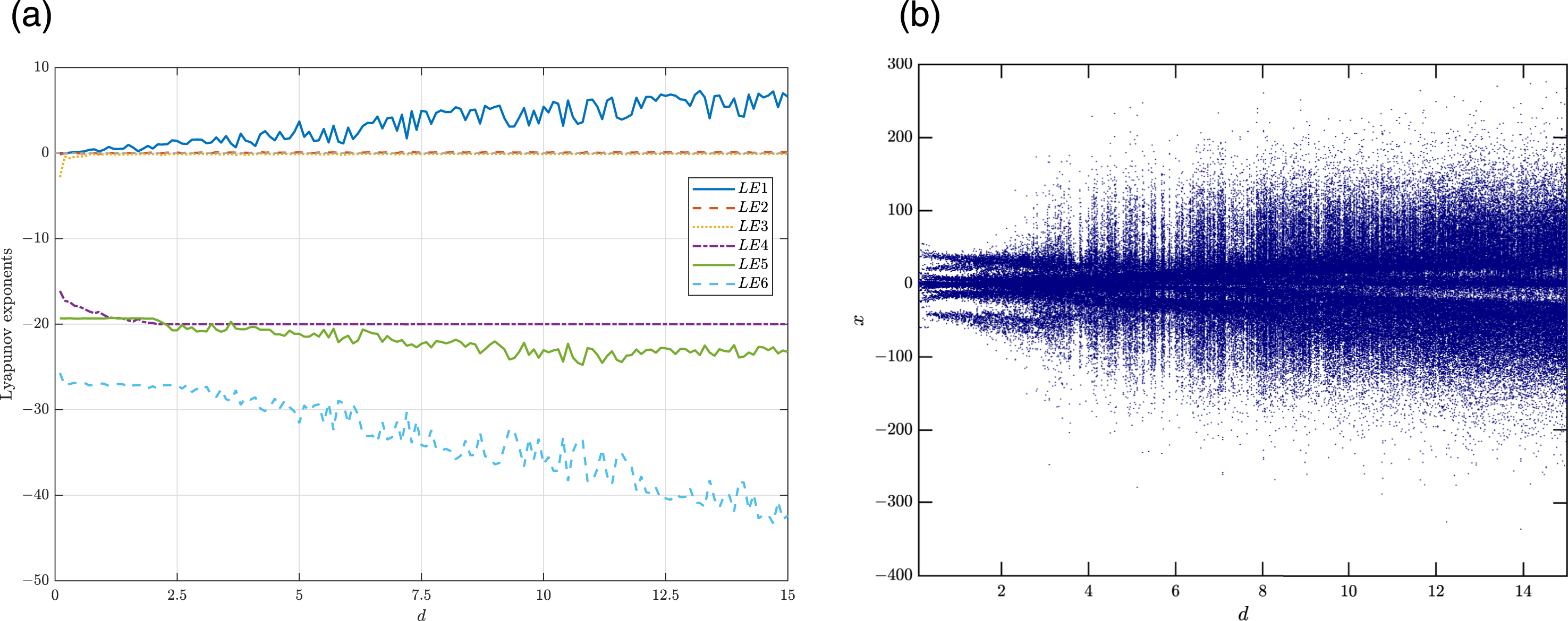
The system’s Lyapunov exponents and bifurcation diagram showing state variable x versus parameter d. (a) Lyapunov exponent spectrum. (b) Bifurcation diagram.

The results show that, when d ∈ (0, 1.1), the system presents a Lyapunov exponent distribution of (+,0, −, −, −, −), indicating a transition into chaotic behavior. When d ∈ (1.1, 15), the system exhibits two positive Lyapunov exponents, signifying that the system enters a hyper-chaotic state.

Case 5

The system parameters are set as a = 16, b = 40, c = 20, d = 8, and β = 2, with α ∈ (0, 10). The corresponding Lyapunov exponent spectrum and the bifurcation diagram of the state variables are shown in Figure 11.

Figure 11.

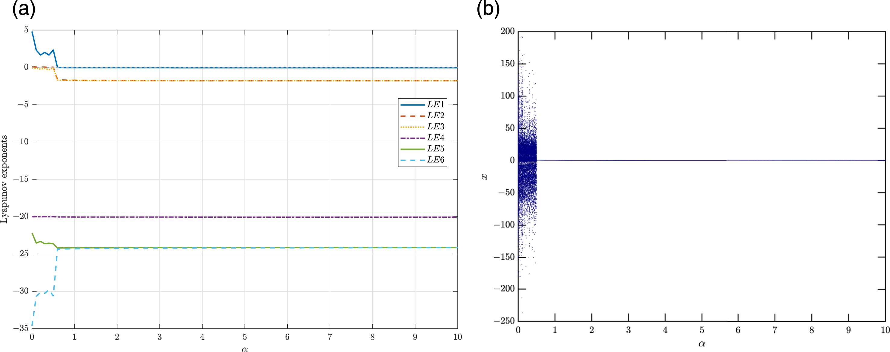
The system’s Lyapunov exponents and bifurcation diagram showing state variable x versus parameter α. (a) Lyapunov exponent spectrum. (b) Bifurcation diagram.

It is observed that the system exhibits stable equilibrium dynamics within the interval α ∈ (0.5, 10), as indicated by the Lyapunov exponent distribution of (0, −, −, −, −, −), and the bifurcation diagram shows that the system converges to a stable equilibrium point. When α ∈ (0, 0.5), the system exhibits two positive Lyapunov exponents, signifying that the system enters a hyper-chaotic state.

Case 6

The system parameters are set as a = 16, b = 40, c = 20, d = 8, and α = 0.01, with β ∈ (0, 10). The corresponding Lyapunov exponent spectrum and the bifurcation diagram of the state variables are shown in Figure 12. It is observed that when β ∈ (0, 10), the system exhibits two positive Lyapunov exponents, indicating that the system remains in a hyper-chaotic state throughout this interval.

Figure 12.

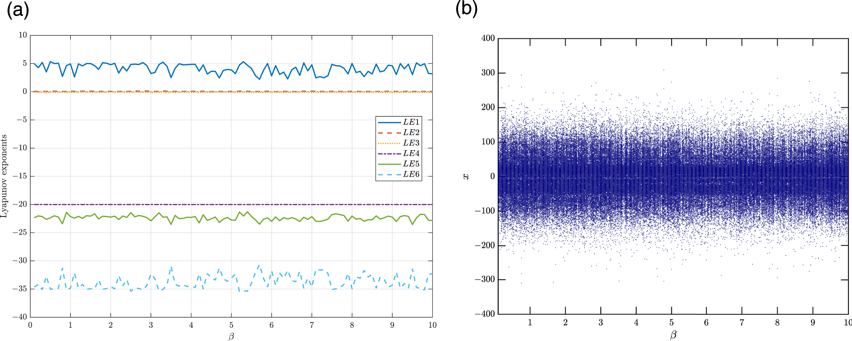
The system’s Lyapunov exponents and bifurcation diagram showing state variable x versus parameter β. (a) Lyapunov exponent spectrum. (b) Bifurcation diagram.

Overall, the above results show that the six-dimensional memristive hyper-chaotic system exhibits rich parameter-dependent dynamical transitions, including stable equilibrium, quasi-periodic, chaotic, and hyper-chaotic states. In particular, hyper-chaotic behavior persists over broad parameter intervals of a, b, c, d, α, and β, demonstrating that the proposed system possesses strong dynamical complexity and a certain degree of robustness with respect to parameter variations.

To complement the bifurcation analysis above and further verify the hyper-chaotic nature of the system, a Poincaré map (Poincaré, 1893) was constructed by recording the intersections of the system trajectory with the hyperplane x = 5 at parameter value a = 16. As illustrated in Figure 13, the resulting cross-section reveals a collection of densely distributed, non-periodic points that exhibit a rich fractal-like geometric structure rather than converging to a finite set of fixed points or a closed curve. This characteristic pattern is a strong indicator of hyper-chaotic dynamics, as periodic or quasi-periodic motions would yield isolated points or smooth closed curves on the Poincaré section, respectively. The irregular and broadly scattered distribution of intersection points, spanning a wide region in the y - z plane, confirms that the system trajectory never repeats itself and sensitively depends on initial conditions. These observations are consistent with the existence of multiple positive Lyapunov exponents, collectively verifying that the system operates in a hyper-chaotic regime with high complexity and unpredictability.

Figure 13.

The system’s Poincaré map and three-dimensional Poincaré section diagram at parameter a = 16 and section x = 5. (a) Poincaré map. (b) Three-dimensional Poincaré section diagram.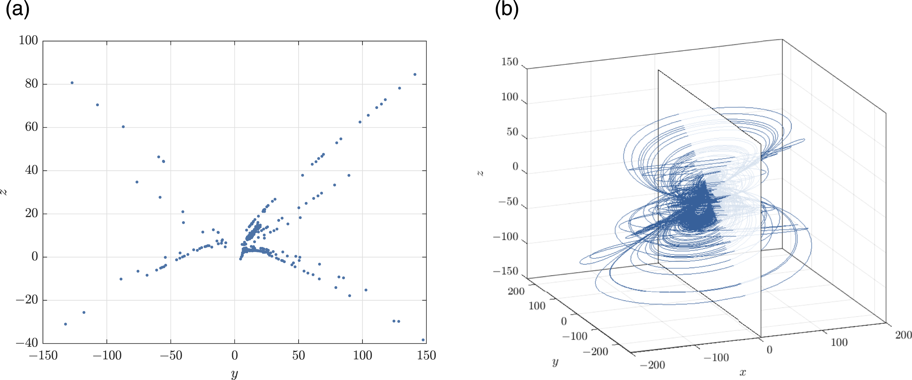

3.5. Time-domain waveform and power spectrum

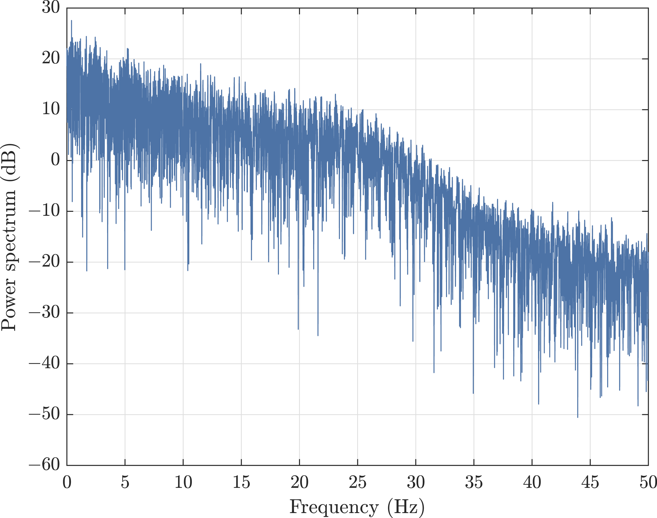
To gain deeper insights into the physical dynamics of the system (6), we analyzed the time-domain waveform of the state variable x by varying its initial value x (0). The corresponding time-domain waveform of x is shown in Figure 14. It can be observed that the system’s state variable x exhibits continuous, non-periodic, and irregular behavior, which is a characteristic feature of chaotic systems. After t > 2, different initial values result in entirely divergent iterative trends, highlighting the system’s sensitivity to initial conditions, this sensitivity is a characteristic of chaotic dynamics. Moreover, through numerical simulations, the power spectrum of system (6) was derived, as shown in Figure 15. The power spectrum exhibits a continuous broadband structure without any dominant discrete spectral peaks, which is a hallmark of aperiodic chaotic motion. The energy is distributed across a wide frequency range, displaying distinct broadband noise characteristics. This observation further confirms that system (6) operates in a hyper-chaotic state. In secure communication applications, such broadband power spectrum features make the system suitable for spread spectrum communication, where the wide frequency distribution enhances resistance to interference and improves signal confidentiality.

Figure 14.

Time-domain waveform of the state variable x.

Figure 15.

Power spectrum of the hyper-chaotic system.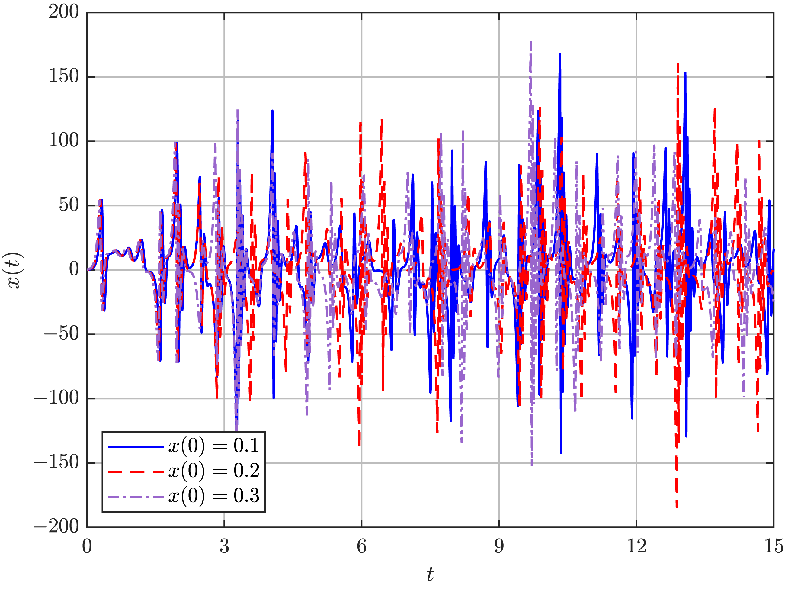

3.6. Circuit implementation of the proposed hyper-chaotic system

To validate the feasibility of the proposed six-dimensional hyper-chaotic system (6), an analog electronic circuit is designed and simulated. The circuit employs LF347BD and AD712CH operational amplifiers with a dual power supply of ±13 V, AD633-type analog multipliers, linear resistors, and capacitors. In the circuit, operational amplifiers are configured primarily as subtractors and integrators to perform the required linear operations, while the multipliers combine the state variables to realize the nonlinear coupling terms.

Based on circuit design principles, a subtractor circuit can be formed by connecting resistors to both the inverting and non-inverting inputs of an operational amplifier. By appropriately configuring the resistor ratios, the output voltage satisfies V_out = −R_f/R_i (V₁ − V₂), enabling weighted subtraction of two input signals. By further incorporating a capacitor as the feedback element in place of the feedback resistor, an integrator circuit is constituted, whose output follows the relation $V_{out} = - 1 / R_{i} C \int_{0}^{t} V_{i n} d t$ . These two fundamental building blocks are combined throughout the circuit to implement each equation of system (6).

As observed in the attractor phase portraits shown in Figure 5, the state variables of system (6) exhibit peak amplitudes of approximately ±300, which would drive the operational amplifiers into saturation if implemented directly in hardware. To resolve this without altering the intrinsic dynamics of the system, a linear amplitude-scaling transformation is introduced. Each state variable is uniformly compressed by a factor of 1000. Since the nonlinear terms involve products of two state variables, they accumulate an additional scaling effect; an extra compression factor of 100 is therefore applied to all nonlinear terms, yielding a total compression of 10⁵ for such terms. By applying Kirchhoff’s Current Law (KCL) and Kirchhoff’s Voltage Law (KVL), and following the circuit analysis approach in Gabelli et al. (2006), we derive the circuit equations as follows

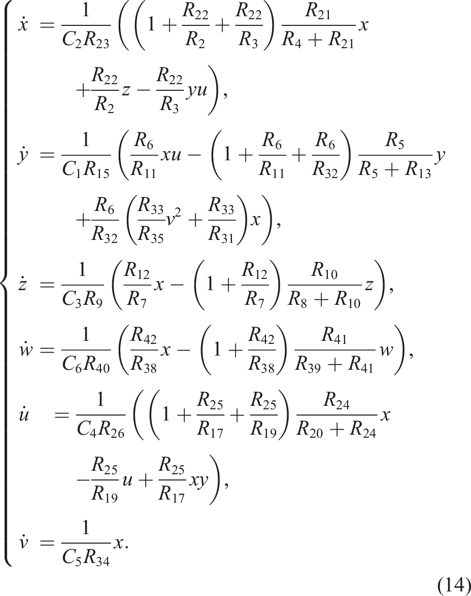
\{\begin{cases} \dot{x} & = \frac{1}{C_{2} R_{23}} ((1 + \frac{R_{22}}{R_{2}} + \frac{R_{22}}{R_{3}}) \frac{R_{21}}{R_{4} + R_{21}} x \\ + \frac{R_{22}}{R_{2}} z - \frac{R_{22}}{R_{3}} y u), \\ \dot{y} & = \frac{1}{C_{1} R_{15}} (\frac{R_{6}}{R_{11}} x u - (1 + \frac{R_{6}}{R_{11}} + \frac{R_{6}}{R_{32}}) \frac{R_{5}}{R_{5} + R_{13}} y \\ + \frac{R_{6}}{R_{32}} (\frac{R_{33}}{R_{35}} v^{2} + \frac{R_{33}}{R_{31}}) x), \\ \dot{z} & = \frac{1}{C_{3} R_{9}} (\frac{R_{12}}{R_{7}} x - (1 + \frac{R_{12}}{R_{7}}) \frac{R_{10}}{R_{8} + R_{10}} z), \\ \dot{w} & = \frac{1}{C_{6} R_{40}} (\frac{R_{42}}{R_{38}} x - (1 + \frac{R_{42}}{R_{38}}) \frac{R_{41}}{R_{39} + R_{41}} w), \\ \dot{u} & = \frac{1}{C_{4} R_{26}} ((1 + \frac{R_{25}}{R_{17}} + \frac{R_{25}}{R_{19}}) \frac{R_{24}}{R_{20} + R_{24}} x \\ - \frac{R_{25}}{R_{19}} u + \frac{R_{25}}{R_{17}} x y), \\ \dot{v} & = \frac{1}{C_{5} R_{34}} x . \end{cases}

(14)

The model of the analog circuit is shown in Figure 16. By comparing the parameters in (14) with those in system (6), the component values shown in Figure 16 can be determined as follows: R₁ = R₇ = R₈ = R₉ = R₁₄ = R₁₆ = R₁₈ = R₂₇ = R₂₈ = R₂₉ = R₃₀ = R₃₆ = R₃₇ = R₃₈ = R₃₉ = R₄₀ = R₄₃ = R₄₄ = 10 KΩ, R₂ = R₁₉ = R₃₂ = R₃₄ = 10 KΩ, R₃ = R₁₇ = R₂₂ = R₂₄ = R₂₅ = 8 KΩ, R₄ = 192 KΩ, R₅ = 40 KΩ, R₆ = R₁₁ = R₁₅ = R₂₃ = R₂₆ = 1 KΩ, R₁₀ = R₁₂ = R₄₁ = R₄₂ = 20 KΩ, R₁₃ = 161 KΩ, R₂₀ = R₃₅ = 200 KΩ, R₂₁ = 16 KΩ, R₃₁ = 3 KΩ, and R₃₃ = 600 KΩ, with C₁ = C₂ = C₃ = C₄ = C₅ = C₆ = 10 nF. In the above component values, KΩ and nF represent kilo-ohms and nanofarads, respectively. The resulting circuit comprises 18 operational amplifiers, 6 capacitors, 5 multipliers, and 44 resistors in total.

Figure 16.

Analog circuit diagram of the hyper-chaotic system.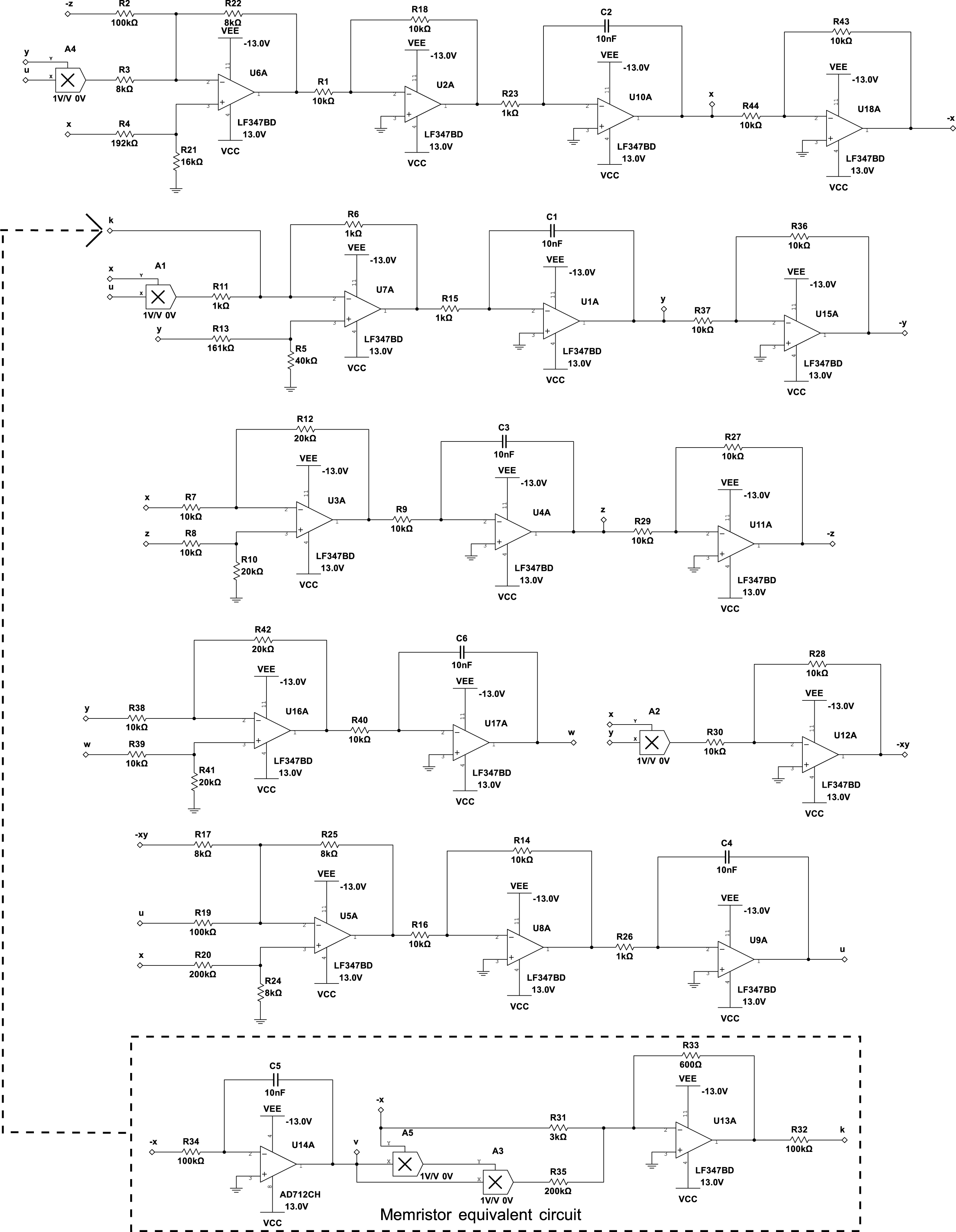

Throughout the simulation process of the electronic circuit, the phase diagram of the attractor, as captured by the oscilloscope, is illustrated in Figure 17. The alignment between the outcomes of the circuit simulation and the numerical simulations strengthens the theoretical foundation of the new hyper-chaotic system. This concordance also substantiates the system’s practical viability.

Figure 17.

Attractor phase diagram of the hyper-chaotic system as observed on the oscilloscope. (a) x-z plane. (b) y-z plane.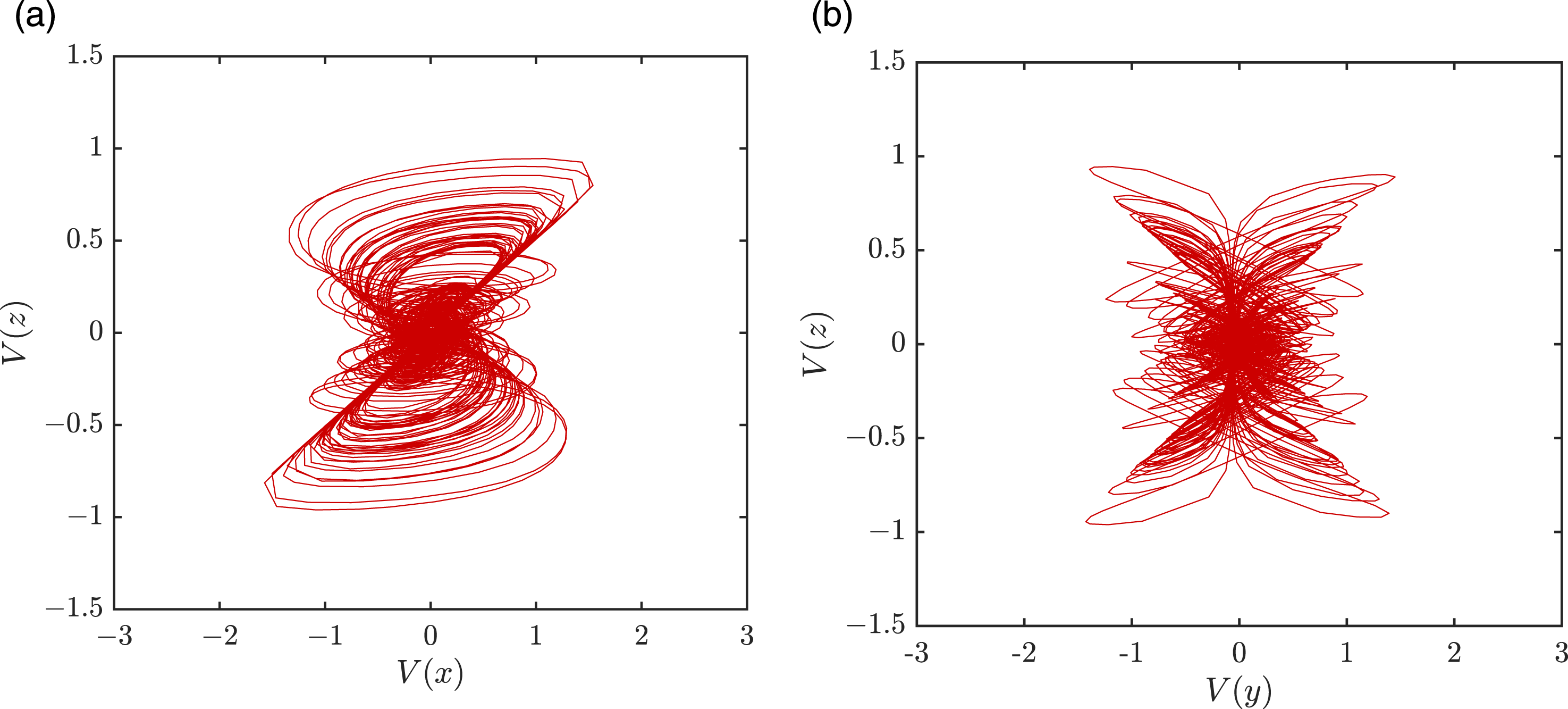

4. Introduction of the dual-time variable dual-pulse intermittent control

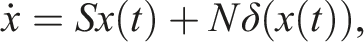
Considering a series of classical nonlinear systems with external control inputs, they are often represented in the form

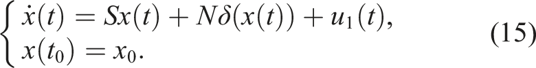
\{\begin{cases} \dot{x} (t) = S x (t) + N δ (x (t)) + u_{1} (t), \\ x (t_{0}) = x_{0} . \end{cases}

(15)

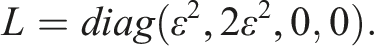
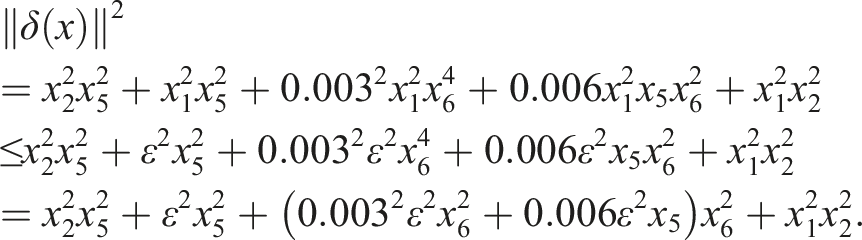
The first equation of (15) dissects the nonlinear system into its constituent elements: a linear segment, a non-linear segment, and an extrinsic control signal, with the state vector denoted by x ∈ Rⁿ. The matrices S, N ∈ R^n×n are constant matrices, and δ: Rⁿ → Rⁿ is a smooth non-linearity fulfilling δ(0) = 0. It is assumed that a diagonal matrix L = diag (l₁, l₂, …, l_n) ≥ 0 exists, ensuring that ‖δ(x)‖² ≤ x^TLx for any x ∈ Rⁿ. The system’s external control perturbation u₁(t), given by the follows

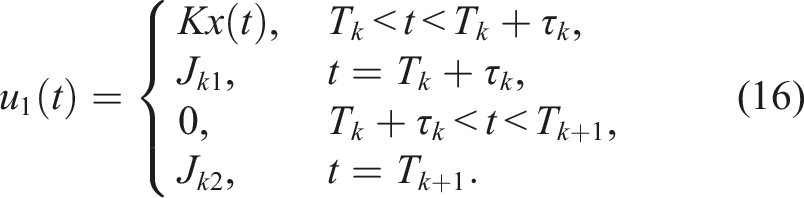
u_{1} (t) = \{\begin{cases} K x (t), & T_{k} < t < T_{k} + τ_{k}, \\ J_{k 1}, & t = T_{k} + τ_{k}, \\ 0, & T_{k} + τ_{k} < t < T_{k + 1}, \\ J_{k 2}, & t = T_{k + 1} . \end{cases}

(16)

Considering the external input control as a piecewise control, therefore, system (15) can be written as

\{\begin{cases} \dot{x} = S x (t) + N δ (x (t)) + K x (t), & T_{k} < t < T_{k} + τ_{k}, \\ x = (I + J_{k 1}) x (t^{-}), & t = T_{k} + τ_{k}, \\ \dot{x} = S x (t) + N δ (x (t)), & T_{k} + τ_{k} < t < T_{k + 1}, \\ x = (I + J_{k 2}) x (t^{-}), & t = T_{k + 1}, \end{cases}

(17)

where k is an integer, K ∈ R^n×n is constant matrices that represent the control intensity, while J_k1 and J_k2 ∈ R^n×n are matrices that represent the impulse intensity, and T_k denotes the variable control period. The system (17) adheres to the right continuity criterion at the point of discontinuity. In addition, τ_k, T_k, J_k1, and J_k2 also satisfy the following equations

\{\begin{cases} \begin{aligned} τ_{k} = \frac{T_{1}}{2} - k η, \\ J_{k i} = 2^{- k} J_{0 i}, i = 1,2, \\ T_{k} = \{\begin{cases} 0, & k = 0, \\ k T_{1} - 2 (k - 1) η, & k > 0, \end{cases} \end{aligned} \end{cases}

(18)

in which η ≥ 0 represents the variance, and τ_k denotes the sequence of control width adjustments, satisfying 0 < τ_k ≤ T₁/2, k = 0, 1, 2, ⋯.

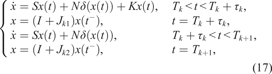
Our goal is to identify the conditions that ensure the stability of system (6). Therefore, it is crucial to determine K, J_0i (i = 1, 2), T₁, and d. The control method in (17) is called dual-time variable dual-pulse intermittent control.

To clearly present our main findings, the following lemmas are essential.

Lemma 1

(Sanchez and Perez, 1999) For any real number matrix ϱ_i(i = 1, 2) ∈ R^N×M, $ϱ_{3} = ϱ_{3}^{T} > 0 \in R^{N \times N}$ , under the condition of a positive scalar γ being present, the following inequality is found to be valid

ϱ_{1}^{T} ϱ_{2} + ϱ_{2}^{T} ϱ_{1} \leq γ ϱ_{1}^{T} ϱ_{3} ϱ_{1} + γ^{- 1} ϱ_{2}^{T} ϱ_{3}^{- 1} ϱ_{2} .

Lemma 2

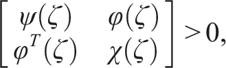
(Boyd et al., 1994) Suppose that ψ(ζ) = ψ^T(ζ), χ(ζ) = χ^T(ζ), and

[\begin{matrix} ψ (ζ) & φ (ζ) \\ φ^{T} (ζ) & χ (ζ) \end{matrix}] > 0,

then, the linear matrix inequality (LMI) described above can be reformulated as the following expression

χ (ζ) > 0, ψ (ζ) - φ (ζ) χ^{- 1} (ζ) φ^{T} (ζ) > 0 .

5. Theoretical analysis and main results

In this section, the exponential stability of system (17) is analyzed using the Lyapunov stability principle. Conditions for determining exponential stability are derived, along with a related corollary.

Theorem 1

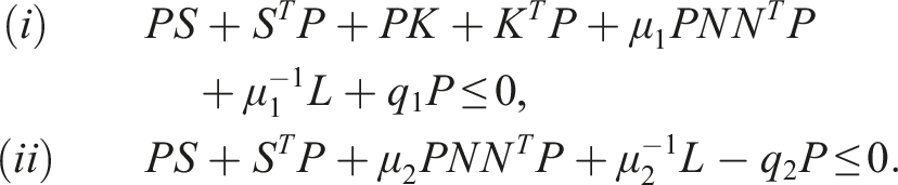
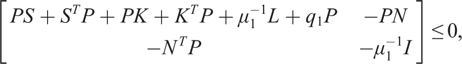
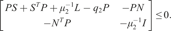
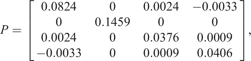
Suppose there exists a symmetric and positive definite matrix P > 0, four positive scalar constants μ₁ > 0, μ₂ > 0, q₁ > 0, and q₂ > 0, satisfying the following conditions

\begin{array}{l} (i) & P S + S^{T} P + P K + K^{T} P + μ_{1} P N N^{T} P \\ + μ_{1}^{- 1} L + q_{1} P \leq 0, \\ (i i) & P S + S^{T} P + μ_{2} P N N^{T} P + μ_{2}^{- 1} L - q_{2} P \leq 0 . \end{array}

Then the origin of system (17) is determined to be exponentially stable, and moreover, for all t > 0,

\begin{aligned} ‖ x (t) ‖ < & \sqrt{\frac{λ_{M} (P)}{λ_{m} (P)}} ‖ x_{0} ‖ \\ \exp (\frac{t + 2 h η + T_{1}}{2 T_{1}} (q_{2} T_{1} + \ln λ_{1} + \ln λ_{2})), \end{aligned}

(19)

where

λ_{1} = \frac{λ_{M} ({(I + J_{k 1})}^{T} P (I + J_{k 1}))}{λ_{m} ({(I + J_{k 1})}^{T} P (I + J_{k 1}))},

and

λ_{2} = \frac{λ_{M} ({(I + J_{k 2})}^{T} P (I + J_{k 2}))}{λ_{m} ({(I + J_{k 2})}^{T} P (I + J_{k 2}))} .

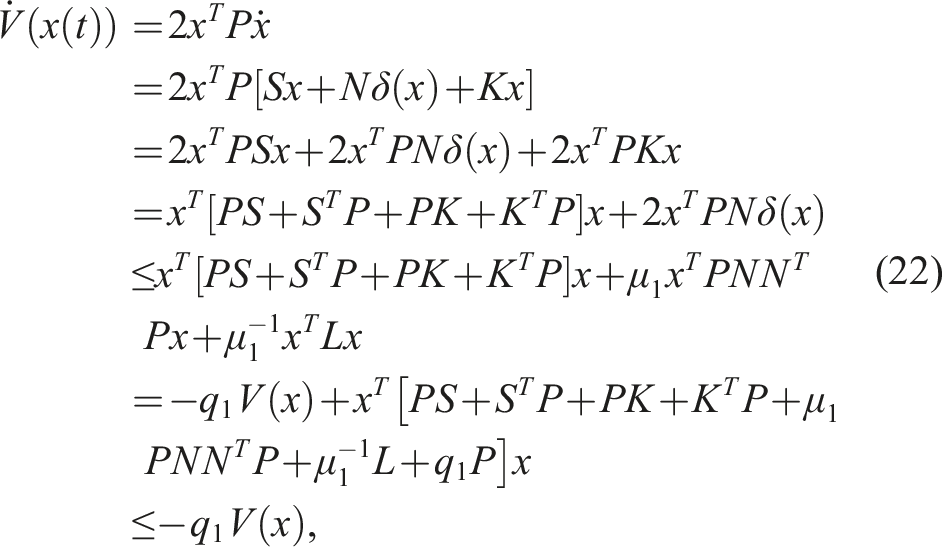
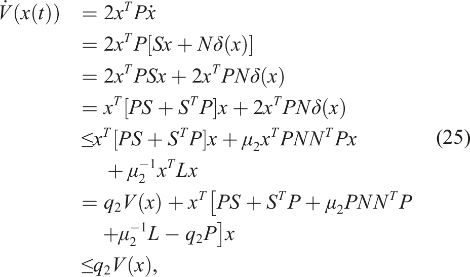
Proof. The Lyapunov function constructed is shown as follows

V (x (t)) = x {(t)}^{T} P x (t),

(20)

moreover, this function satisfies

λ_{m} (P) ‖ x (t) ‖^{2} \leq V (x (t)) \leq λ_{M} (P) ‖ x (t) ‖^{2} .

(21)

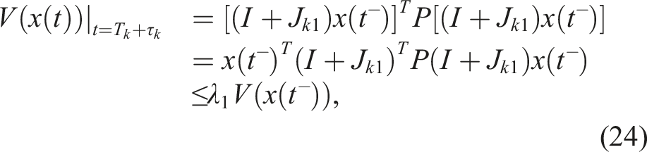
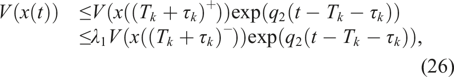
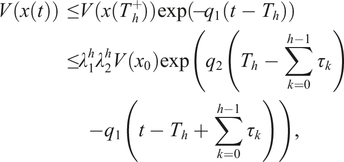
When T_k<t<T_k+τ_k, the state of system (17) can be calculated and estimated by using Lemma 1 and (20) as follows

\begin{align} \dot{V} (x (t)) & = 2 x^{T} P \dot{x} \\ = 2 x^{T} P [S x + N δ (x) + K x] \\ = 2 x^{T} P S x + 2 x^{T} P N δ (x) + 2 x^{T} P K x \\ = x^{T} [P S + S^{T} P + P K + K^{T} P] x + 2 x^{T} P N δ (x) \\ \leq x^{T} [P S + S^{T} P + P K + K^{T} P] x + μ_{1} x^{T} P N N^{T} \\ P x + μ_{1}^{- 1} x^{T} L x \\ = - q_{1} V (x) + x^{T} [P S + S^{T} P + P K + K^{T} P + μ_{1} \\ P N N^{T} P + μ_{1}^{- 1} L + q_{1} P] x \\ \leq - q_{1} V (x), \end{align}

(22)

where

P S + S^{T} P + P K + K^{T} P + μ_{1} P N N^{T} P + μ_{1}^{- 1} L + q_{1} P \leq 0

. Therefore, it can be obtained that

V (x (t)) \leq V (x (T_{k}^{+})) \exp (- q_{1} (t - T_{k})),

(23)

suppose that t = T_k + τ_k, then

\begin{align} V (x (t)) |_{t = T_{k} + τ_{k}} & = {[(I + J_{k 1}) x (t^{-})]}^{T} P [(I + J_{k 1}) x (t^{-})] \\ = x {(t^{-})}^{T} {(I + J_{k 1})}^{T} P (I + J_{k 1}) x (t^{-}) \\ \leq λ_{1} V (x (t^{-})), \end{align}

(24)

where

λ_{1} = λ_{M} ({(I + J_{k 1})}^{T} P (I + J_{k 1})) / λ_{m} ({(I + J_{k 1})}^{T} P (I + J_{k 1}))

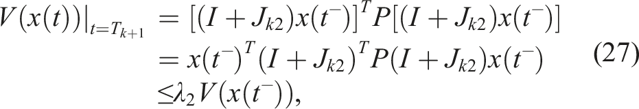
When T_k + τ_k < t < T_k+1, the following conclusion can be derived

\begin{align} \dot{V} (x (t)) & = 2 x^{T} P \dot{x} \\ = 2 x^{T} P [S x + N δ (x)] \\ = 2 x^{T} P S x + 2 x^{T} P N δ (x) \\ = x^{T} [P S + S^{T} P] x + 2 x^{T} P N δ (x) \\ \leq x^{T} [P S + S^{T} P] x + μ_{2} x^{T} P N N^{T} P x \\ + μ_{2}^{- 1} x^{T} L x \\ = q_{2} V (x) + x^{T} [P S + S^{T} P + μ_{2} P N N^{T} P \\ + μ_{2}^{- 1} L - q_{2} P] x \\ \leq q_{2} V (x), \end{align}

(25)

where

P S + S^{T} P + μ_{2} P N N^{T} P + μ_{2}^{- 1} L - q_{2} P \leq 0

Therefore, it can be obtained that

\begin{align} V (x (t)) & \leq V (x ({(T_{k} + τ_{k})}^{+})) \exp (q_{2} (t - T_{k} - τ_{k})) \\ \leq λ_{1} V (x ({(T_{k} + τ_{k})}^{-})) \exp (q_{2} (t - T_{k} - τ_{k})), \end{align}

(26)

suppose that t = T_k+1, then

\begin{align} V (x (t)) |_{t = T_{k + 1}} & = {[(I + J_{k 2}) x (t^{-})]}^{T} P [(I + J_{k 2}) x (t^{-})] \\ = x {(t^{-})}^{T} {(I + J_{k 2})}^{T} P (I + J_{k 2}) x (t^{-}) \\ \leq λ_{2} V (x (t^{-})), \end{align}

(27)

where

λ_{2} = λ_{M} ({(I + J_{k 2})}^{T} P (I + J_{k 2})) / λ_{m} ({(I + J_{k 2})}^{T} P (I + J_{k 2}))

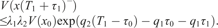
From (22)–(27), by employing mathematical induction, a series of conclusions can be sequentially established as follows.

Case 1: k = 0.

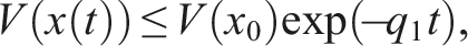
Subcase 1: When 0 < t < τ₀, it can be obtained that

V (x (t)) \leq V (x_{0}) \exp (- q_{1} t),

therefore

V (x (τ_{0}^{-})) \leq V (x_{0}) \exp (q_{1} τ_{0}) .

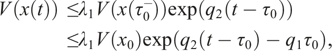
Subcase 2: When τ₀ ≤ t < T₁, it can be obtained that

\begin{array}{l} V (x (t)) & \leq λ_{1} V (x (τ_{0}^{-})) \exp (q_{2} (t - τ_{0})) \\ \leq λ_{1} V (x_{0}) \exp (q_{2} (t - τ_{0}) - q_{1} τ_{0}), \end{array}

therefore

V (x (T_{1}^{-})) \leq λ_{1} V (x_{0}) \exp (q_{2} (T_{1} - τ_{0}) - q_{1} τ_{0}) .

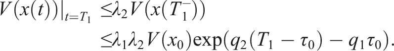
Subcase 3: When t = T₁, it can be obtained that

\begin{array}{l} V (x (t)) |_{t = T_{1}} & \leq λ_{2} V (x (T_{1}^{-})) \\ \leq λ_{1} λ_{2} V (x_{0}) \exp (q_{2} (T_{1} - τ_{0}) - q_{1} τ_{0}) . \end{array}

Case 2: k = 1.

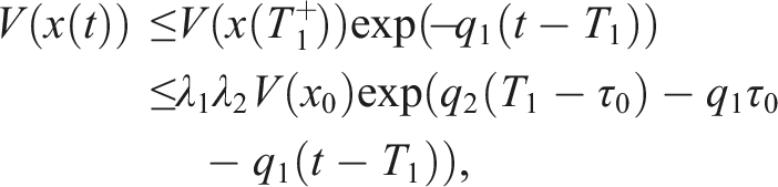
Subcase 1: When T₁ < t < T₁ + τ₁, it can be obtained that

\begin{array}{l} V (x (t)) & \leq V (x (T_{1}^{+})) \exp (- q_{1} (t - T_{1})) \\ \leq λ_{1} λ_{2} V (x_{0}) \exp (q_{2} (T_{1} - τ_{0}) - q_{1} τ_{0} \\ - q_{1} (t - T_{1})), \end{array}

therefore

\begin{array}{l} V (x {(T_{1} + τ_{1})}^{-}) \\ \leq λ_{1} λ_{2} V (x_{0}) \exp (q_{2} (T_{1} - τ_{0}) - q_{1} τ_{0} - q_{1} τ_{1}) . \end{array}

Subcase 2: When T₁ + τ₁ ≤ t < T₂, it can be obtained that

\begin{array}{l} V (x (t)) & \leq λ_{1} V (x {(T_{1} + τ_{1})}^{-}) \exp (q_{2} (t - T_{1} - τ_{1})) \\ \leq λ_{1}^{2} λ_{2} V (x_{0}) \exp (q_{2} (t - T_{1} - τ_{1}) - q_{2} (T_{1} - τ_{0}) \\ - q_{1} τ_{0} - q_{1} τ_{1}) \\ = λ_{1}^{2} λ_{2} V (x_{0}) \exp (q_{2} (t - τ_{1} - τ_{0}) - q_{1} τ_{0} - q_{1} τ_{1}), \end{array}

therefore

\begin{array}{l} V (x (T_{2}^{-})) \\ \leq λ_{1}^{2} λ_{2} V (x_{0}) \exp (q_{2} (T_{2} - τ_{1} - τ_{0}) - q_{1} τ_{0} - q_{1} τ_{1}) . \end{array}

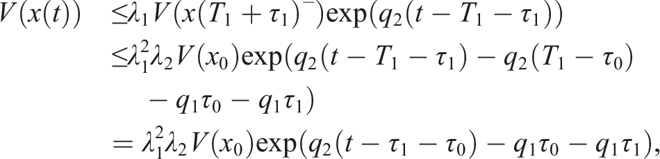
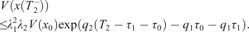
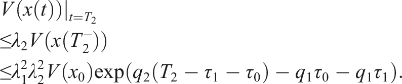
Subcase 3: When t = T₂, it can be obtained that

\begin{array}{l} V (x (t)) |_{t = T_{2}} \\ \leq λ_{2} V (x (T_{2}^{-})) \\ \leq λ_{1}^{2} λ_{2}^{2} V (x_{0}) \exp (q_{2} (T_{2} - τ_{1} - τ_{0}) - q_{1} τ_{0} - q_{1} τ_{1}) . \end{array}

Case h + 1: k = h.

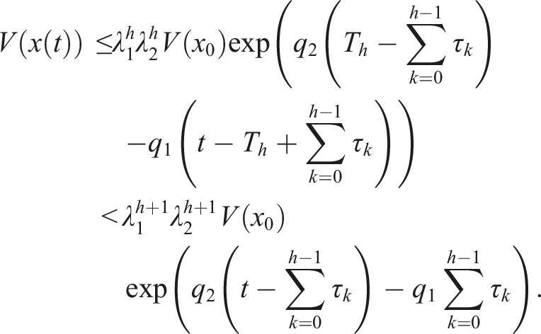
Subcase 1: When T_h < t < T_h + τ_h, it can be obtained that

\begin{array}{l} V (x (t)) & \leq V (x (T_{h}^{+})) \exp (- q_{1} (t - T_{h})) \\ \leq λ_{1}^{h} λ_{2}^{h} V (x_{0}) \exp (q_{2} (T_{h} - \sum_{k = 0}^{h - 1} τ_{k}) \\ - q_{1} (t - T_{h} + \sum_{k = 0}^{h - 1} τ_{k})), \end{array}

therefore

\begin{array}{l} V (x {(T_{h} + τ_{h})}^{-}) \\ \leq λ_{1}^{h} λ_{2}^{h} V (x_{0}) \exp (q_{2} (T_{h} - \sum_{k = 0}^{h - 1} τ_{k}) - q_{1} \sum_{k = 0}^{h} τ_{k}) . \end{array}

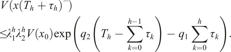
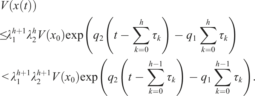
Subcase 2: When T_h + τ_h ≤ t < T_h+1, it can be obtained that

\begin{array}{l} V (x (t)) \\ \leq λ_{1} V (x {(T_{h} + τ_{h})}^{-}) \exp (q_{2} (t - T_{h} - τ_{h})) \\ \leq λ_{1}^{h + 1} λ_{2}^{h} V (x_{0}) \exp (q_{2} (t - \sum_{k = 0}^{h} τ_{k}) - q_{1} \sum_{k = 0}^{h} τ_{k}), \end{array}

therefore

\begin{array}{l} V (x (T_{h + 1}^{-})) \\ \leq λ_{1}^{h + 1} λ_{2}^{h} V (x_{0}) \exp (q_{2} (T_{h + 1} - \sum_{k = 0}^{h} τ_{k}) - q_{1} \sum_{k = 0}^{h} τ_{k}) . \end{array}

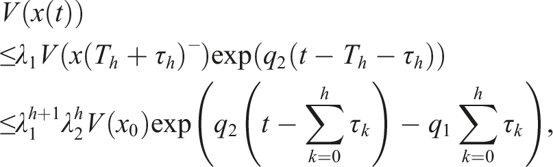
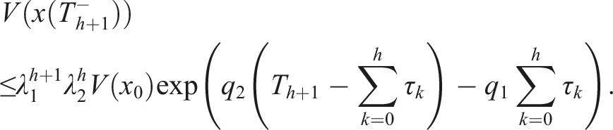
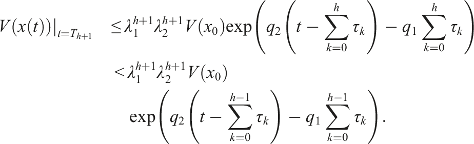
Subcase 3: When t = T_h+1, it can be obtained that

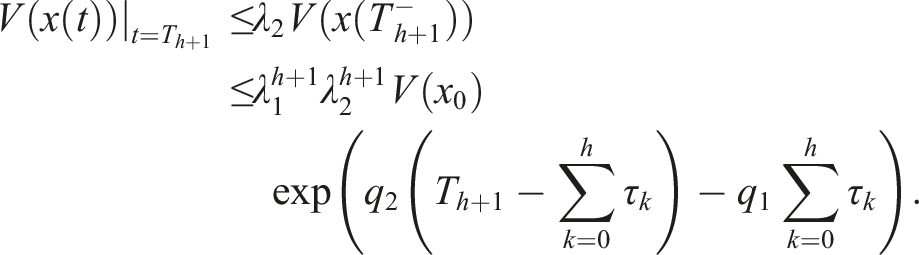
\begin{array}{l} {V (x (t))|}_{t = T_{h + 1}} & \leq λ_{2} V (x (T_{h + 1}^{-})) \\ \leq λ_{1}^{h + 1} λ_{2}^{h + 1} V (x_{0}) \\ \exp (q_{2} (T_{h + 1} - \sum_{k = 0}^{h} τ_{k}) - q_{1} \sum_{k = 0}^{h} τ_{k}) . \end{array}

Furthermore, when T_h < t < T_h + τ_h, that is, 0 < t − T_h < τ_h, it follows that

\begin{array}{l} V (x (t)) & \leq λ_{1}^{h} λ_{2}^{h} V (x_{0}) \exp (q_{2} (T_{h} - \sum_{k = 0}^{h - 1} τ_{k}) \\ - q_{1} (t - T_{h} + \sum_{k = 0}^{h - 1} τ_{k})) \\ < λ_{1}^{h + 1} λ_{2}^{h + 1} V (x_{0}) \\ \exp (q_{2} (t - \sum_{k = 0}^{h - 1} τ_{k}) - q_{1} \sum_{k = 0}^{h - 1} τ_{k}) . \end{array}

When T_h + τ_h ≤ t < T_h+1, that is, τ_h < t − T_h, the following can be inferred

\begin{array}{l} V (x (t)) \\ \leq λ_{1}^{h + 1} λ_{2}^{h} V (x_{0}) \exp (q_{2} (t - \sum_{k = 0}^{h} τ_{k}) - q_{1} \sum_{k = 0}^{h} τ_{k}) \\ < λ_{1}^{h + 1} λ_{2}^{h + 1} V (x_{0}) \exp (q_{2} (t - \sum_{k = 0}^{h - 1} τ_{k}) - q_{1} \sum_{k = 0}^{h - 1} τ_{k}) . \end{array}

When t = T_h+1, the following can be inferred

\begin{array}{l} V (x (t)) |_{t = T_{h + 1}} & \leq λ_{1}^{h + 1} λ_{2}^{h + 1} V (x_{0}) \exp (q_{2} (t - \sum_{k = 0}^{h} τ_{k}) - q_{1} \sum_{k = 0}^{h} τ_{k}) \\ < λ_{1}^{h + 1} λ_{2}^{h + 1} V (x_{0}) \\ \exp (q_{2} (t - \sum_{k = 0}^{h - 1} τ_{k}) - q_{1} \sum_{k = 0}^{h - 1} τ_{k}) . \end{array}

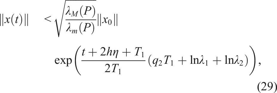
Thus, when T_h < t ≤ T_h+1, that is, (t + 2hη)/T₁ ≤ h + 1 < (t + 2hη + T₁)/T₁, it can be deduced that

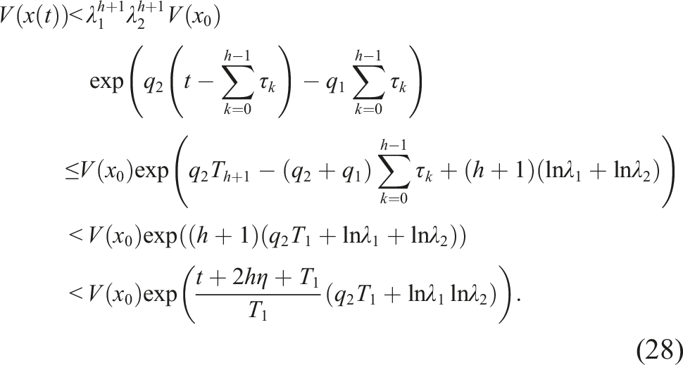
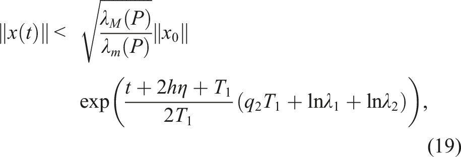
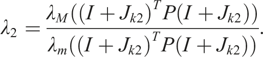
\begin{align} V (x (t)) & < λ_{1}^{h + 1} λ_{2}^{h + 1} V (x_{0}) \\ \exp (q_{2} (t - \sum_{k = 0}^{h - 1} τ_{k}) - q_{1} \sum_{k = 0}^{h - 1} τ_{k}) \\ \leq V (x_{0}) \exp (q_{2} T_{h + 1} - (q_{2} + q_{1}) \sum_{k = 0}^{h - 1} τ_{k} + (h + 1) (\ln λ_{1} + \ln λ_{2})) \\ < V (x_{0}) \exp ((h + 1) (q_{2} T_{1} + \ln λ_{1} + \ln λ_{2})) \\ < V (x_{0}) \exp (\frac{t + 2 h η + T_{1}}{T_{1}} (q_{2} T_{1} + \ln λ_{1} \ln λ_{2})) . \end{align}

(28)

Additionally, equation (28) can be approximately evaluated using (21), leading to the conclusion, for all t > 0

\begin{align} ‖ x (t) ‖ & < \sqrt{\frac{λ_{M} (P)}{λ_{m} (P)}} ‖ x_{0} ‖ \\ \exp (\frac{t + 2 h η + T_{1}}{2 T_{1}} (q_{2} T_{1} + \ln λ_{1} + \ln λ_{2})), \end{align}

(29)

which ends the proof. ■

Corollary 1

From Lemma 2, the primary conditions enunciated in Theorem 1 are reformulated as the following LMIs

[\begin{matrix} P S + S^{T} P + P K + K^{T} P + μ_{1}^{- 1} L + q_{1} P & - P N \\ - N^{T} P & - μ_{1}^{- 1} I \end{matrix}] \leq 0,

[\begin{matrix} P S + S^{T} P + μ_{2}^{- 1} L - q_{2} P & - P N \\ - N^{T} P & - μ_{2}^{- 1} I \end{matrix}] \leq 0 .

6. Examples of numerical simulation analysis

Example 1

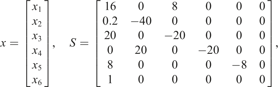
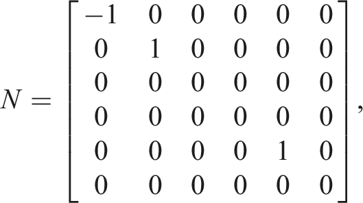
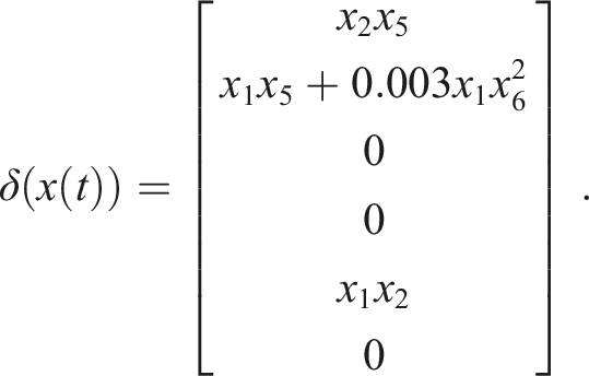
In this paper, the new dual-time variable dual-pulse intermittent control strategy proposed in Section 4 is applied to stabilize the memristive hyper-chaotic system (6) constructed in Section 2. Through a series of numerical simulations, it is demonstrated that the hyper-chaotic system ultimately converges to exponential stability, thereby confirming the effectiveness of this control method.

Based on the analytical exposition in Section 4, system (6) can be rewritten in the following form

\dot{x} = S x (t) + N δ (x (t)),

in which

x = [\begin{matrix} x_{1} \\ x_{2} \\ x_{3} \\ x_{4} \\ x_{5} \\ x_{6} \end{matrix}], S = [\begin{matrix} 16 & 0 & 8 & 0 & 0 & 0 \\ 0.2 & - 40 & 0 & 0 & 0 & 0 \\ 20 & 0 & - 20 & 0 & 0 & 0 \\ 0 & 20 & 0 & - 20 & 0 & 0 \\ 8 & 0 & 0 & 0 & - 8 & 0 \\ 1 & 0 & 0 & 0 & 0 & 0 \end{matrix}],

N = [\begin{matrix} - 1 & 0 & 0 & 0 & 0 & 0 \\ 0 & 1 & 0 & 0 & 0 & 0 \\ 0 & 0 & 0 & 0 & 0 & 0 \\ 0 & 0 & 0 & 0 & 0 & 0 \\ 0 & 0 & 0 & 0 & 1 & 0 \\ 0 & 0 & 0 & 0 & 0 & 0 \end{matrix}],

and

δ (x (t)) = [\begin{matrix} x_{2} x_{5} \\ x_{1} x_{5} + 0.003 x_{1} x_{6}^{2} \\ 0 \\ 0 \\ x_{1} x_{2} \\ 0 \end{matrix}] .

Assuming that x₁(t) ∈ (−ɛ, ɛ), where ɛ > 0 is a constant, the subsequent outcome is derived

\begin{array}{l} ‖ δ (x) ‖^{2} \\ = x_{2}^{2} x_{5}^{2} + x_{1}^{2} x_{5}^{2} + 0.00 3^{2} x_{1}^{2} x_{6}^{4} + 0.006 x_{1}^{2} x_{5} x_{6}^{2} + x_{1}^{2} x_{2}^{2} \\ \leq x_{2}^{2} x_{5}^{2} + ε^{2} x_{5}^{2} + 0.00 3^{2} ε^{2} x_{6}^{4} + 0.006 ε^{2} x_{5} x_{6}^{2} + x_{1}^{2} x_{2}^{2} \\ = x_{2}^{2} x_{5}^{2} + ε^{2} x_{5}^{2} + (0.00 3^{2} ε^{2} x_{6}^{2} + 0.006 ε^{2} x_{5}) x_{6}^{2} + x_{1}^{2} x_{2}^{2} . \end{array}

Let x (0) = [0.3,0.3,0.3,0.3,0.3,0.3]^T, timing diagram and time domain waveforms of the state variable, as depicted in Figure 18, from which it can be inferred that |x₁(t)| ≤ 60, |x₂(t)| ≤ 60, |x₅(t)| ≤ 70 and |x₆(t)| ≤ 120, then

L = d i a g (0, ε^{2}, 0,0,2 ε^{2}, 0.5496 ε^{2}) .

Figure 18.

Time domain waveforms of four state variables.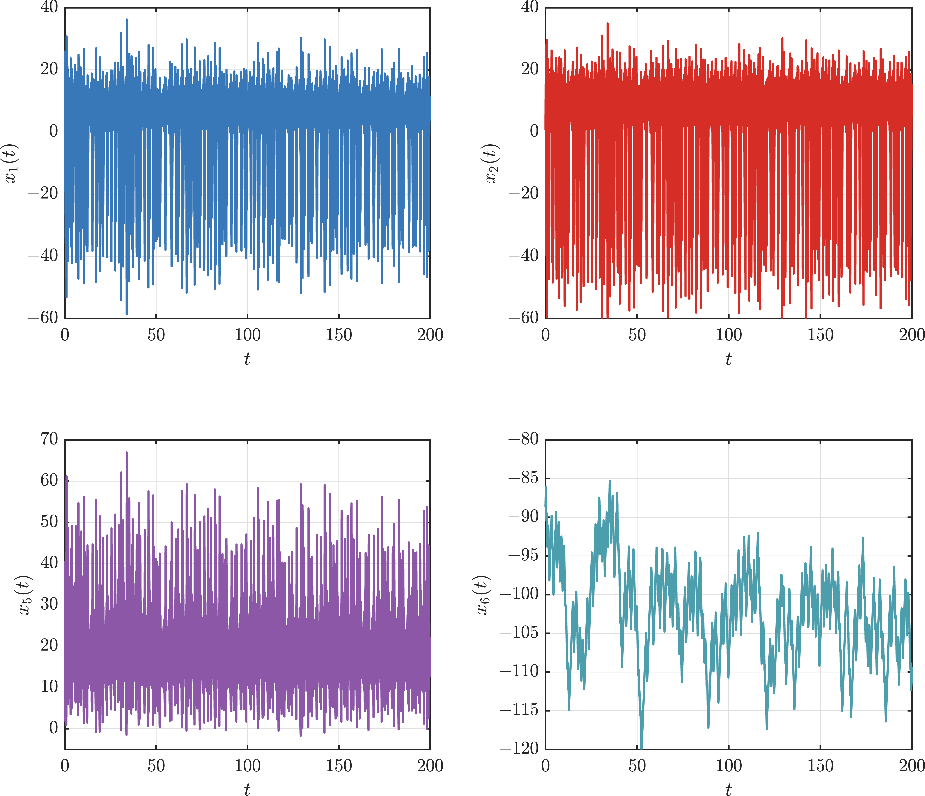

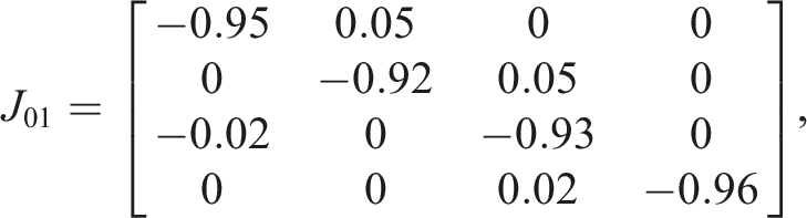
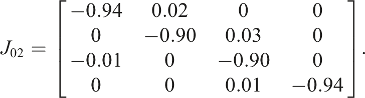
Selecting

K = d i a g (- 60, - 60, - 60, - 60, - 60, - 60) .

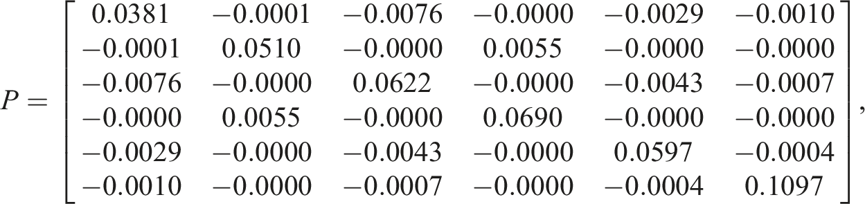
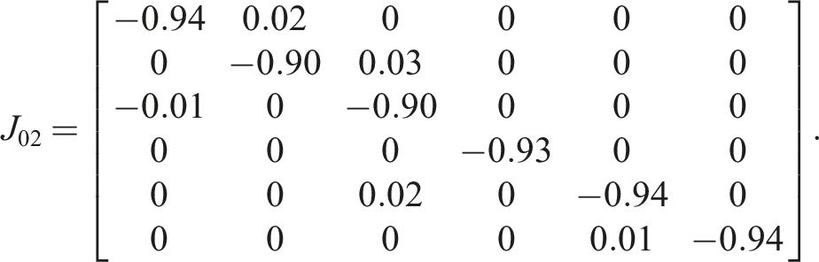
Motivated by the time-parameter settings used in the related intermittent and impulsive control schemes in Refs. (Li et al., 2023; Xie et al., 2022), several admissible pairs (T₁, η), including (0.4, 0.0004), (0.04, 0.0004), and (0.03, 0.0004), are tested in the present system. Among them, some choices led to slower convergence or poorer numerical performance. Therefore, we finally choose T₁ = 0.02 and η = 0.0004, by solving the two LMIs in Corollary 1 and inequality (( t + 2 hη + T₁)/T₁ )(q₂T₁ + ln λ₁ + ln λ₂) < 0, then the following feasible solution is obtained

q_{1} = 35, q_{2} = 85, μ_{1} = 2500, μ_{2} = 2500,

P = [\begin{matrix} 0.0381 & - 0.0001 & - 0.0076 & - 0.0000 & - 0.0029 & - 0.0010 \\ - 0.0001 & 0.0510 & - 0.0000 & 0.0055 & - 0.0000 & - 0.0000 \\ - 0.0076 & - 0.0000 & 0.0622 & - 0.0000 & - 0.0043 & - 0.0007 \\ - 0.0000 & 0.0055 & - 0.0000 & 0.0690 & - 0.0000 & - 0.0000 \\ - 0.0029 & - 0.0000 & - 0.0043 & - 0.0000 & 0.0597 & - 0.0004 \\ - 0.0010 & - 0.0000 & - 0.0007 & - 0.0000 & - 0.0004 & 0.1097 \end{matrix}],

J_{01} = [\begin{matrix} - 0.95 & 0.05 & 0 & 0 & 0 & 0 \\ 0 & - 0.92 & 0.05 & 0 & 0 & 0 \\ - 0.02 & 0 & - 0.92 & 0 & 0 & 0 \\ 0 & 0 & 0 & - 0.95 & 0 & 0 \\ 0 & 0 & 0.02 & 0 & - 0.96 & 0 \\ 0 & 0 & 0 & 0 & 0.02 & - 0.96 \end{matrix}],

and

J_{02} = [\begin{matrix} - 0.94 & 0.02 & 0 & 0 & 0 & 0 \\ 0 & - 0.90 & 0.03 & 0 & 0 & 0 \\ - 0.01 & 0 & - 0.90 & 0 & 0 & 0 \\ 0 & 0 & 0 & - 0.93 & 0 & 0 \\ 0 & 0 & 0.02 & 0 & - 0.94 & 0 \\ 0 & 0 & 0 & 0 & 0.01 & - 0.94 \end{matrix}] .

Based on the relevant data, we have plotted the trend graph of pulse width variation for the control strategy presented in this study, as shown in Figure 19. Observations indicate that the width of both the controlled and uncontrolled segments exhibits a monotonically decreasing trend. To ensure the continued effectiveness of the control strategy, a threshold for width variation has been established. Once the change in control width exceeds this preset threshold, the pulse width will no longer change and will remain in intermittent control mode.

Figure 19.

Variation trend graph of intermittent control width with respect to periodic iteration.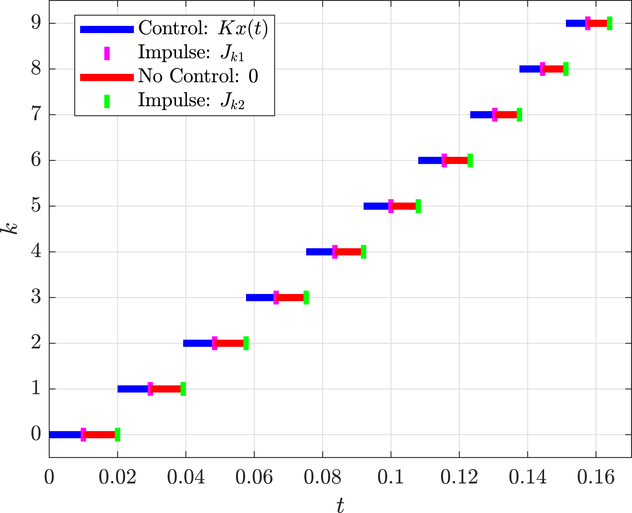

Ultimately, based on the findings established herein, it is affirmed that the validity of Theorem 1 is confirmed. Moreover, the trajectory of the state response for the governed six-dimensional memristive hyper-chaotic system is depicted in Figure 20, from which it can be observed that the control method proposed in this paper effectively stabilizes the hyper-chaotic system established in Section 2. Through comparative analysis with Li et al. (2023), it can be concluded that the proposed method enables the system to reach a stable state in a markedly shorter time, with a faster convergence rate and a narrower fluctuation range around the steady-state value. This illustrates that the control approach delineated within this paper possesses notable superiority with respect to the expeditiousness of response, stability, and control accuracy, thereby proving its higher reliability and effectiveness in practical applications.

Figure 20.

State response curves of controlled system. (a) State response curves of proposed strategy. (b) State response curves of Ref. (Li et al., 2023).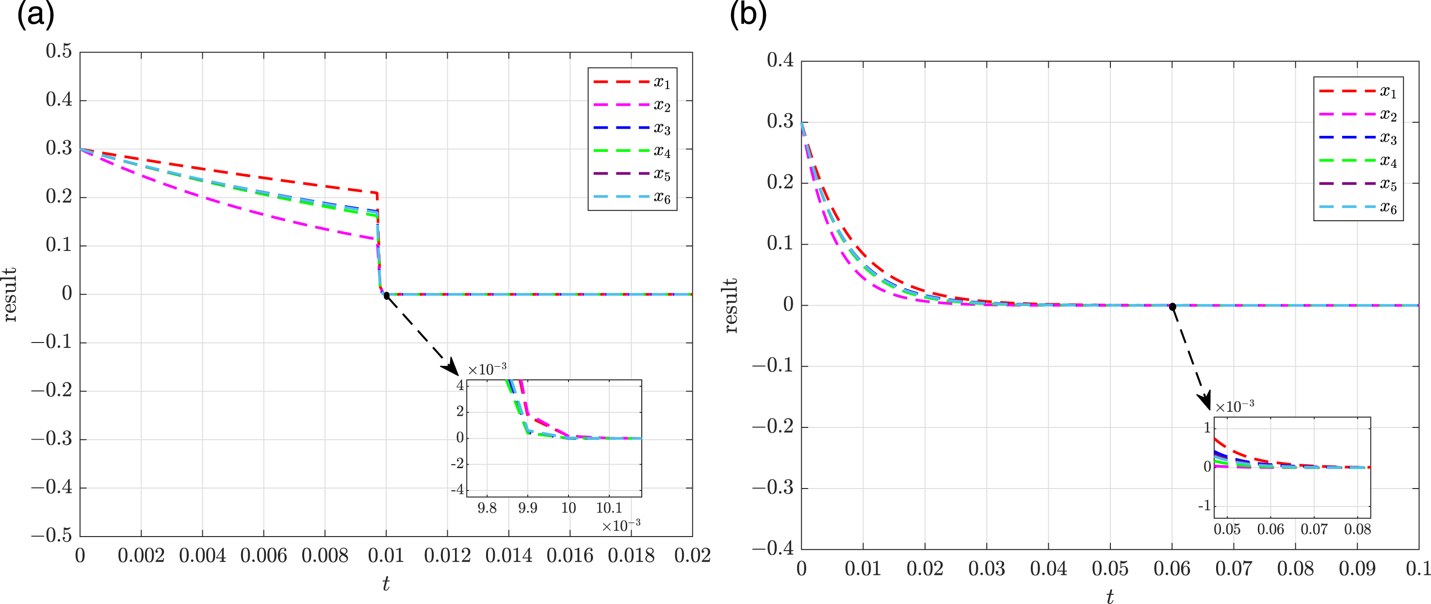

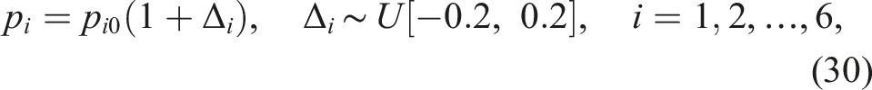
To further examine the robustness of the proposed dual-time variable dual-pulse intermittent control strategy, additional numerical simulations are carried out for the six-dimensional memristive hyper-chaotic system under bounded simultaneous parameter uncertainties. Specifically, the plant parameters are modeled as

p_{i} = p_{i 0} (1 + Δ_{i}), Δ_{i} \sim U [- 0.2, 0.2], i = 1,2, \dots, 6,

(30)

where p₁, p₂, p₃, p₄, p₅, and p₆ denote the perturbed parameters a, b, c, d, α, and β, respectively, p₁₀, p₂₀, p₃₀, p₄₀, p₅₀, and p₆₀ denote their corresponding nominal parameters a, b, c, d, α, and β, respectively, the random variable Δ_i follows a uniform distribution on the interval [−0.2, 0.2], and all controller parameters remain unchanged. To provide a more convincing robustness evaluation, 50 Monte Carlo runs are performed with randomly generated time-invariant parameter deviations. The simulation results show that all 50 runs are successfully stabilized, corresponding to a success rate of 100%. Moreover, both the mean and maximum settling times are 0.0098 s, while the mean and maximum final state norms are 1.929,231 × 10⁻¹³ and 2.176,104 × 10⁻¹³, respectively. A representative perturbed case selected from the Monte Carlo simulations is shown in Figure 21. It can be observed that the state trajectories still converge rapidly to the equilibrium point, and the corresponding norm response remains almost identical to that of the nominal case. These results demonstrate that the proposed control strategy maintains excellent stabilization performance even in the presence of relatively large parameter uncertainties of up to ±20%.

Figure 21.

Robustness test of the proposed control strategy for the six-dimensional memristive hyper-chaotic system under bounded parameter perturbations of up to ±20%. (a) State responses under a representative perturbed case. (b) State norm comparison between the nominal and perturbed cases.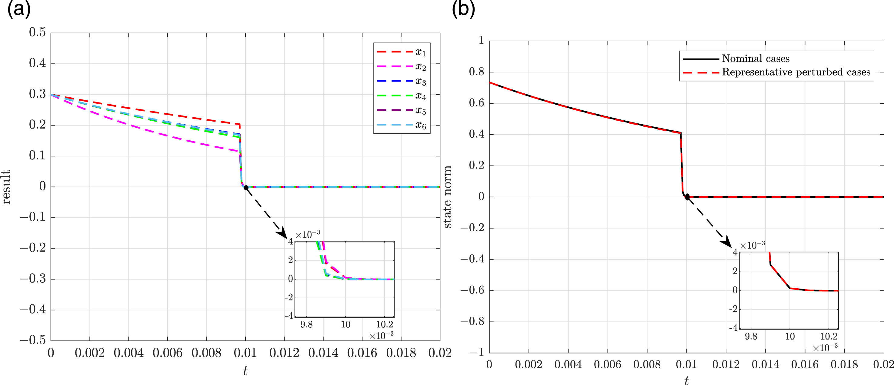

To further investigate the robustness of the proposed control strategy against external disturbances, additional simulations are carried out for the six-dimensional memristive hyper-chaotic system under measurement noise interference. In this test, the system parameters and controller parameters remain unchanged, while additive Gaussian noise is introduced into the measured states used for feedback control, with noise model

\hat{x} (t) = x (t) + σ n (t),

(31)

where

\hat{x} = {[{\hat{x}}_{1}, {\hat{x}}_{2}, {\hat{x}}_{3}, {\hat{x}}_{4}, {\hat{x}}_{5}, {\hat{x}}_{6}]}^{T}

denotes the state vector after the addition of measurement noise, and x denotes the original state vector, n(t) ∼ N (0, I), N (0, I) denotes the multivariate Gaussian distribution with zero mean and identity covariance matrix and σ = 0.01. To provide a more convincing robustness evaluation, 50 Monte Carlo runs are performed under independent measurement-noise cases. The simulation results show that all 50 runs are successfully stabilized, corresponding to a success rate of 100%. Moreover, the mean and maximum settling times are 0.0098 s and 0.0099 s, respectively, while the mean and maximum final state norms are 4.595,829 × 10⁻³ and 8.455,246 × 10⁻³, respectively. A representative noisy case selected from the Monte Carlo simulations is shown in Figure 22. It can be observed that the state trajectories still converge rapidly to a small neighborhood of the equilibrium point, although small residual fluctuations remain in the steady stage due to persistent measurement noise. The corresponding state norm response also remains close to that of the nominal case. These results indicate that the proposed control strategy remains effective in the presence of measurement noise.

Example 2

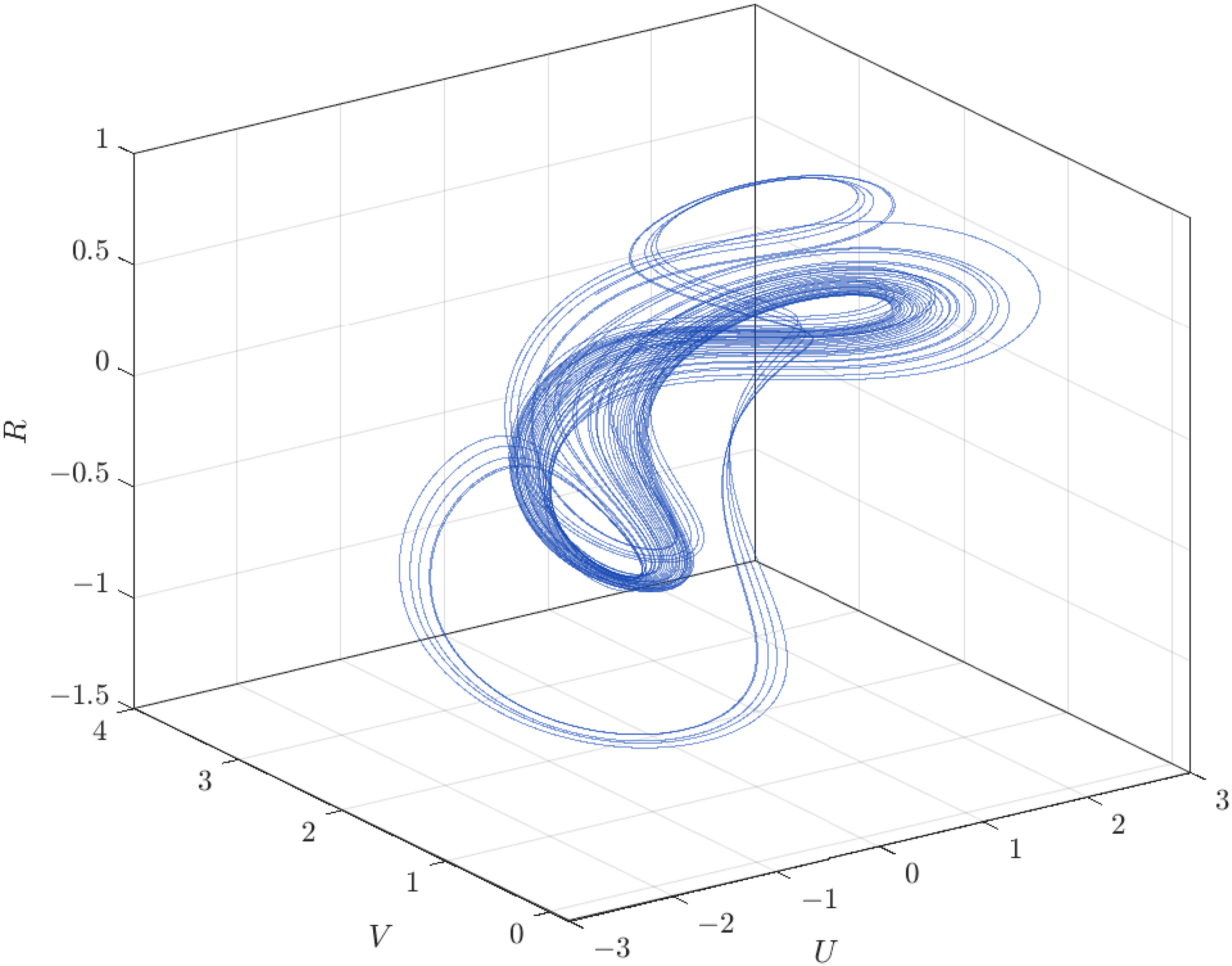
To further validate the applicability of the proposed control strategy to real-world dynamical systems, we apply it to the four-dimensional hyper-chaotic financial system proposed by Borah et al. (2025). This model captures the intricate nonlinear interactions among interest rates, investment demand, price indices, and exchange rates in a financial market, and has been shown to exhibit rich hyper-chaotic dynamics characterized by at least two positive Lyapunov exponents. The model is described by the following system of autonomous ordinary differential equations

\{\begin{cases} \dot{U} = W + (V - s) U - R, \\ \dot{V} = 1 - r V - U^{2}, \\ \dot{W} = - U - e W + p R, \\ \dot{R} = m U V - g R, \end{cases}

(32)

where U, V, W, and R denote the interest rate, investment demand, price index, and exchange rate, respectively. The parameter s represents the saving amount coefficient in the bank, r is the cost per investment, e is the elasticity of demand, p is the import price pass-through rate, m is the economic activity sensitivity factor for the exchange rate, and g is the exchange rate adjustment factor. All parameters s, r, e, p, m, and g are non-negative constants. With parameters s = 0.9, r = 0.2, e = 1.5, p = 1, m = 0.2, and g = 0.3, the initial conditions of the system are set as [0.1,0.1,0.1,0.1]^T, the attractor phase portrait of the system is shown in Figure 23. It can be observed that prior to the application of control measures, the hyper-chaotic financial system dynamics exhibit chaotic behavior.

Figure 22.

Robustness test of the proposed control strategy for the six-dimensional memristive hyper-chaotic system under measurement noise interference. (a) State responses under a representative noisy case. (b) State norm comparison between the nominal and noisy cases.

Figure 23.

The attractor phase portrait of the system (32).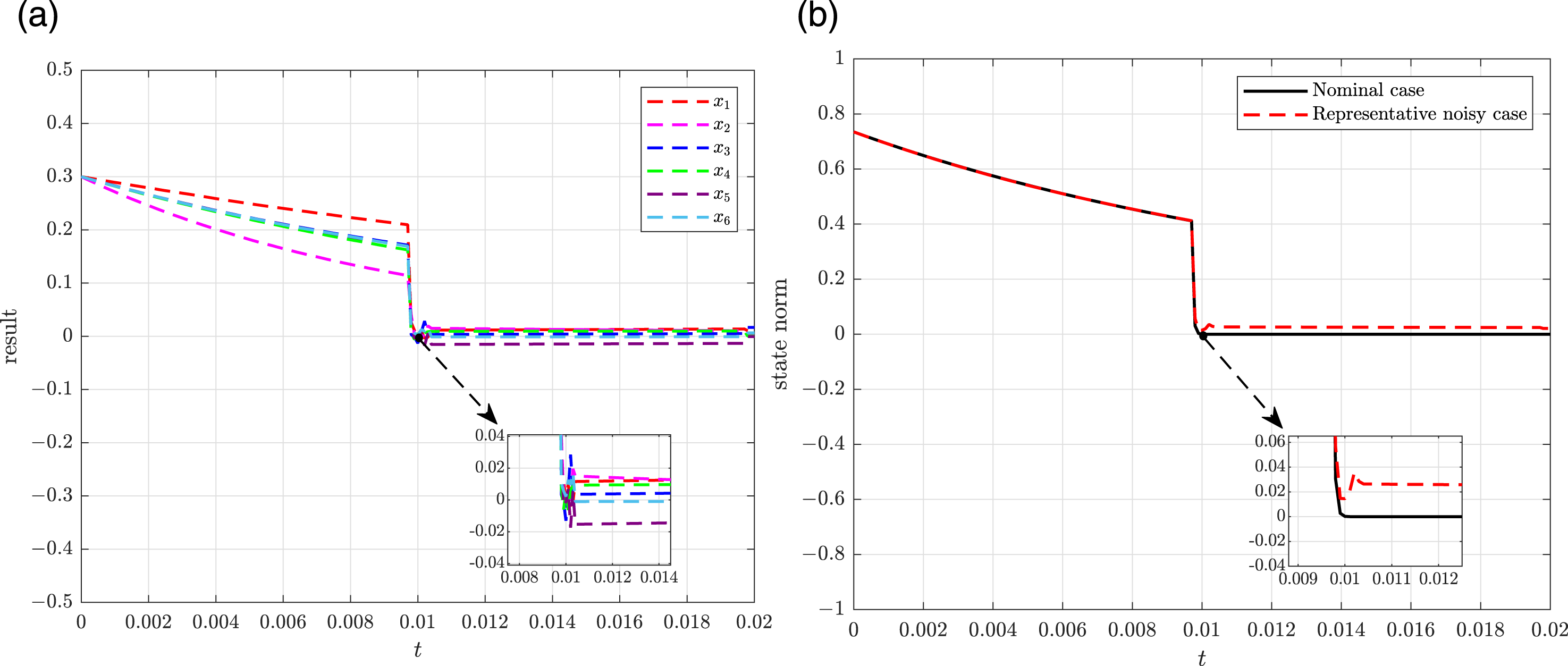

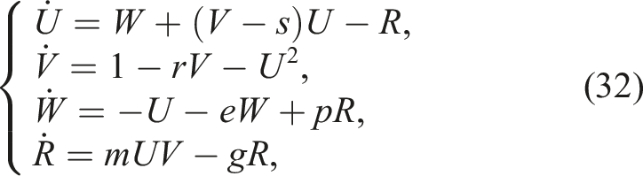
Similarly, the system (32) can be reformulated into the general form of a nonlinear system as described in Section 4, from which we can derive the following equations

‖ δ (x) ‖^{2} = 2 U^{2} V^{2} + U^{4} .

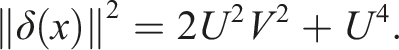
Assuming U(t) ∈ (−ɛ, ɛ), where ɛ > 0 is a constant, we can derive the following results

L = d i a g (ε^{2}, 2 ε^{2}, 0,0) .

Selecting

K = d i a g (- 20, - 20, - 20, - 20) .

Assuming that T₁ = 0.01, η = 0.005, by solving the two LMIs in Corollary 1 and inequality t + 2 hη + T₁/T₁ (q₂T₁ + ln λ₁ + ln λ₂) < 0, then the ensuing collection of viable solutions is derived

q_{1} = 25, q_{2} = 35, μ_{1} = 10, μ_{2} = 10,

P = [\begin{matrix} 0.0824 & 0 & 0.0024 & - 0.0033 \\ 0 & 0.1459 & 0 & 0 \\ 0.0024 & 0 & 0.0376 & 0.0009 \\ - 0.0033 & 0 & 0.0009 & 0.0406 \end{matrix}],

J_{01} = [\begin{matrix} - 0.95 & 0.05 & 0 & 0 \\ 0 & - 0.92 & 0.05 & 0 \\ - 0.02 & 0 & - 0.93 & 0 \\ 0 & 0 & 0.02 & - 0.96 \end{matrix}],

and

J_{02} = [\begin{matrix} - 0.94 & 0.02 & 0 & 0 \\ 0 & - 0.90 & 0.03 & 0 \\ - 0.01 & 0 & - 0.90 & 0 \\ 0 & 0 & 0.01 & - 0.94 \end{matrix}] .

Under the aforementioned conditions, we employ the dual-time variable dual-pulse intermittent control strategy. The time response curves of the state variables for the hyperchaotic financial system (32) are depicted in Figure 24. It is observed that all state variables, including the interest rate U, investment demand V, price index W, and exchange rate R, are effectively stabilized within a relatively short period, with each variable trending towards zero. This outcome not only verifies the feasibility of our control strategy in suppressing the complex hyper-chaotic dynamics inherent in financial systems but also introduces a novel approach for the stabilization and regulation of nonlinear financial models, demonstrating its potential in practical applications. This work provides new insights into the modeling and control of hyper-chaotic financial systems, serving as a reference for future research and practice.

Figure 24.

The time response curves of the system (32).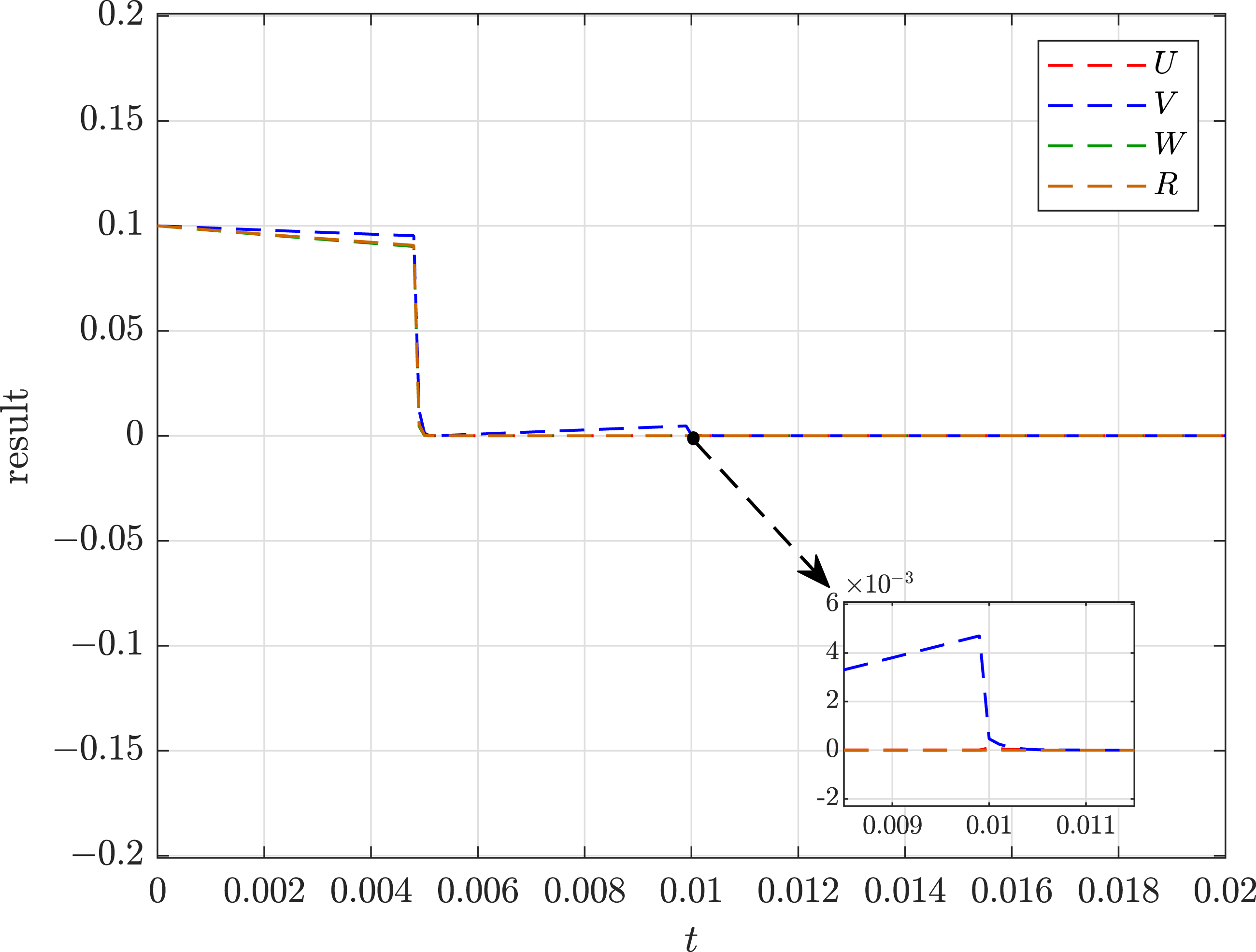

7. Conclusions

This paper constructs a novel six-dimensional memristive hyper-chaotic system derived from a five-dimensional chaotic system by integrating a flux-controlled memristor as a nonlinear feedback element. The inclusion of this memristor significantly enhances the system’s dynamic complexity, as rigorously confirmed through Lyapunov exponent spectra, Kaplan–Yorke dimension calculation, bifurcation diagrams, Poincaré maps, and power spectral analysis. The physical implementability of the system is further validated via analog circuit simulation, ensuring consistency between theoretical analysis and practical implementation.

Based on these findings, a dual-time variable dual-pulse intermittent control strategy is proposed. Different from traditional fixed-width intermittent control methods, this strategy allows the control width sequences of both the controlled and uncontrolled phases to decrease monotonically with a fixed step size across successive control cycles, while two independent impulsive gain matrices are deployed at the phase boundaries of each cycle with exponentially decaying amplitudes. This enables the controller to flexibly adjust control intensity in response to the evolving system trajectory, greatly improving convergence speed, stability, and control accuracy. Using Lyapunov stability theory and Linear Matrix Inequality (LMI) techniques, sufficient conditions for exponential stability are rigorously established.

The numerical simulation results validate the efficacy of the proposed control strategy, effectively stabilizing both the newly constructed six-dimensional memristive hyper-chaotic system and the four-dimensional hyper-chaotic financial system. Compared with existing methods, the proposed approach achieves a markedly shorter stabilization time and a narrower steady-state fluctuation range, demonstrating superior reliability and broad applicability to nonlinear dynamical models in both engineering and economic contexts. Nevertheless, the present study is mainly limited to an integer-order continuous-time framework with numerical and circuit-level validation, and its hardware-oriented realization and secure-communication deployment still require further investigation. Future work will therefore focus on incorporating event-triggered mechanisms to improve control efficiency, extending the proposed framework to fractional-order memristive hyper-chaotic systems, and exploring more hardware-friendly secure communication architectures. In particular, motivated by the recent development of gain-tunable high-dimensional discrete hyper-chaotic systems for image encryption and FPGA-oriented implementation (Yang and Feng, 2026), we will further investigate the integration of hyper-chaotic modeling, control design, secure communication, and hardware realization.

Footnotes

ORCID iD

Yuming Feng

Funding

The authors disclosed receipt of the following financial support for the research, authorship, and/or publication of this article: This work is sponsored by the Science and Technology Research Program of Chongqing Municipal Education Commission, P.R. China (Grant Nos. KJQN202201221, KJQN202501242), the Natural Science Foundation of Chongqing, P.R. China (Grant Nos. CSTB2024NSCQ-LZX0083, CSTB2024NSCQ-LZX0119), the National Natural Science Foundation of China (Grant No. 12261030), and the Chongqing Graduate Research and Innovation Program (Grant No. CYS25847).

Declaration of conflicting interests

The authors declared no potential conflicts of interest with respect to the research, authorship, and/or publication of this article.

References

Abba

Teh

Alawida

(2024) Towards accurate keyspace analysis of chaos-based image ciphers. Multimedia Tools and Applications 83(33): 79047–79066. https://doi.org/10.1007/s11042-024-18628-8

Abou El Qassime

Nhaila

Bahatti

, et al. (2025) Advanced speech encryption method leveraging a hidden hyperchaotic attractor and its synchronization with robust adaptive sliding mode control. Nonlinear Dynamics 113(12): 15553–15578. https://doi.org/10.1007/s11071-025-10948-0

Borah

Dehingia

Phukan

, et al. (2025) Study on a hyper-chaotic financial system with synchronization. Mathematical and Computer Modelling of Dynamical Systems 31(1): 2495916. https://doi.org/10.1080/13873954.2025.2495916

Boyd

El Ghaoui

Feron

, et al. (1994) Linear Matrix Inequalities in System and Control Theory. Society for Industrial and Applied Mathematics. https://doi.org/10.1137/1.9781611970777

Chen

(2025) Optimal synchronization of higher-order dynamical networks. Artificial Intelligence Science and Engineering 1(1): 31–36. https://doi.org/10.23919/AISE.2025.000003

Chua

(1971) Memristor-the missing circuit element. IEEE Transactions on Circuit Theory 18(5): 507–519. https://doi.org/10.1109/TCT.1971.1083337

Ding

Shi

Erkan

, et al. (2026a) Design of a three-dimensional logistic map and its application to seafood image encryption. The Journal of Supercomputing 82(4): 225. Available at: https://doi.org/10.1007/s11227-025-08196-5

Ding

Wang

Zhu

, et al. (2026b) SRA: a sine-based reconstruction approach to improve 2D chaotic map performance. The European Physical Journal Plus 141(2): 182. Available at: https://doi.org/10.1140/epjp/s13360-026-07421-1

Frederickson

Kaplan

Yorke

, et al. (1983) The Liapunov dimension of strange attractors. Journal of Differential Equations 49(2): 185–207. https://doi.org/10.1016/0022-0396(83)90011-6

10.

Gabelli

Fève

Berroir

, et al. (2006) Violation of Kirchhoff’s laws for a coherent RC circuit. Science 313(5786): 499–502. https://doi.org/10.1126/science.1126940

11.

Gao

HHC

Erkan

, et al. (2025a) A 3D memristive cubic map with dual discrete memristors: design, implementation, and application in image encryption. IEEE Transactions on Circuits and Systems for Video Technology 35(8): 7706–7718. Available at: https://doi.org/10.1109/TCSVT.2025.3545868

12.

Gao

Zhang

, et al. (2025b) Encrypt a story: a video segment encryption method based on the discrete sinusoidal memristive rulkov neuron. IEEE Transactions on Dependable and Secure Computing 22(6): 8011–8024. Available at: https://doi.org/10.1109/TDSC.2025.3603570

13.

Gao

Shi

, et al. (2026a) A memristor-based neural network circuit with classical conditioning and fear generalization. IEEE Transactions on Consumer Electronics 72: 3213–3224. Available at: https://doi.org/10.1109/TCE.2026.3663359

14.

Gao

Song

Cao

, et al. (2026b) Biologically plausible memristive decision-making circuit for adaptive control in industrial autonomous navigation. IEEE Transactions on Industrial Informatics 22: 4801–4812. Available at: https://doi.org/10.1109/TII.2026.3668794

15.

Gokyildirim

Calgan

Demirtas

(2024) Fractional-order sliding mode control of a 4D memristive chaotic system. Journal of Vibration and Control 30(7-8): 1604–1620. https://doi.org/10.1177/10775463231166187

16.

Jie

Wang

Zhang

, et al. (2025) Model construction and image encryption application of chaotic system under the influence of memristor and unknown parameters. Nonlinear Dynamics 113(11): 13859–13883. https://doi.org/10.1007/s11071-024-10854-x

17.

Kopp

Samuilik

(2025) Hidden attractors in a new 4D memristor-based hyperchaotic system: dynamical analysis, circuit design, synchronization, and its applications. Mathematics 13(17): 2838. https://doi.org/10.3390/math13172838

18.

Lai

Liu

, et al. (2025a) Generating grid multiscroll memristive chua’s circuit and its predefined-time synchronization for secure communication. IEEE Transactions on Circuits and Systems I: Regular Papers 72(10): 5947–5956. Available at: https://doi.org/10.1109/TCSI.2025.3541635

19.

Lai

Wang

Huang

(2025b) Diverse dynamical behaviors and predefined-time synchronization of a simple memristive chaotic system. Acta Physica Sinica 74(20): 200501. Available at: https://doi.org/10.7498/aps.74.20250954

20.

Lai

Wang

(2024) Finite and fixed-time synchronization of memristive chaotic systems based on sliding mode reaching law. Acta Physica Sinica 73(18): 180503. https://doi.org/10.7498/aps.73.20241013

21.

Lai

Wang

(2026) Predefined-time synchronization of cyclic memristive neural networks via adaptive sliding mode control: comparative analysis and application in secure communication. Communications in Nonlinear Science and Numerical Simulation 156: 109734. https://doi.org/10.1016/j.cnsns.2026.109734

22.

Wang

(2025) Optimal impulse control and impulse game for continuous-time deterministic systems: a review. Artificial Intelligence Science and Engineering 1(3): 208–219. https://doi.org/10.23919/AISE.2025.000014

23.

Peng

Cao

(2020) Lyapunov stability for impulsive systems via event-triggered impulsive control. IEEE Transactions on Automatic Control 65(11): 4908–4913. https://doi.org/10.1109/tac.2020.2964558

24.

Cao

, et al. (2023) Periodically intermittent control of memristor-based hyper-chaotic bao-like system. Mathematics 11(5): 1264. https://doi.org/10.3390/math11051264

25.

Liu

(2020) Exponential stabilization of delayed inertial memristive neural networks via aperiodically intermittent control strategy. IEEE Transactions on Systems, Man, and Cybernetics: Systems 52(1): 448–458. https://doi.org/10.1109/tsmc.2020.3002960

26.

Liu

Yang

Liu

, et al. (2020) Stabilization to exponential input-to-state stability via aperiodic intermittent control. IEEE Transactions on Automatic Control 66(6): 2913–2919. https://doi.org/10.1109/tac.2020.3014637

27.

Lorenz

(1963) Deterministic nonperiodic flow. Journal of the Atmospheric Sciences 20(2): 130–141. https://doi.org/10.1175/1520-0469(1963)020(0130:DNF)2.0.CO;2

28.

Mirzaei

Aslmostafa

Asadollahi

, et al. (2023) Fast fixed-time sliding mode control for synchronization of chaotic systems with unmodeled dynamics and disturbance; applied to memristor-based oscillator. Journal of Vibration and Control 29(9-10): 2129–2143. https://doi.org/10.1177/10775463221075116

29.

Mobayen

Mostafaee

Alattas

, et al. (2024) A new hyperchaotic system: circuit realization, nonlinear analysis and synchronization control. Physica Scripta 99(10): 105204. https://doi.org/10.1088/1402-4896/ad71fc

30.

Kong

(2026) Stabilization of switched neutral networked systems: fixed-time intermittent control framework. International Journal of Robust and Nonlinear Control 36(3): 1379–1392. https://doi.org/10.1002/rnc.70210

31.

Ozpolat

Gulten

(2024) Synchronization and application of a novel hyperchaotic system based on adaptive observers. Applied Sciences 14(3): 1311. https://doi.org/10.3390/app14031311

32.

Poincaré

(1893) Les Méthodes Nouvelles de la Mécanique Céleste, Tome II. Gauthier-Villars. Digital Library of India Item 2015.153619.

33.

Rong

Chedjou

, et al. (2024) A special memristive diode-bridge-based hyperchaotic hyperjerk autonomous circuit with three positive lyapunov exponents. Chaos, Solitons & Fractals 189: 115704. https://doi.org/10.1016/j.chaos.2024.115704

34.

Sanchez

Perez

(1999) Input-to-state stability (iss) analysis for dynamic neural networks. IEEE Transactions on circuits and systems I: Fundamental Theory and Applications 46(11): 1395–1398. https://doi.org/10.1109/81.802844

35.

Song

Tong

(2025) Inverse reinforcement learning optimal control for takagi-sugeno fuzzy systems. Artificial Intelligence Science and Engineering 1(2): 134–146. https://doi.org/10.23919/AISE.2025.000010

36.

Strukov

Snider

Stewart

, et al. (2008) The missing memristor found. Nature 453(7191): 80–83. https://doi.org/10.1038/nature06932

37.

Tan

Feng

(2025) A new pre-defined smooth mode control for chaotic synchronization with exponential function. Chaos, Solitons & Fractals 201: 117158. https://doi.org/10.1016/j.chaos.2025.117158

38.

Tang

Shi

Yang

, et al. (2025) Finite-time synchronization of coupled fractional-order systems via intermittent it-2 fuzzy control. IEEE Transactions on Systems, Man, and Cybernetics: Systems 55(3): 2022–2032. https://doi.org/10.1109/TSMC.2024.3518513

39.

Zhang

, et al. (2025) Event-triggered impulsive control for input-to-state stability of nonlinear time-delay system with delayed impulse. Mathematical Biosciences and Engineering 22: 876–896.

40.

Ulutas

(2025) A novel memristor-based hyperchaotic hybrid encryption system with dna for image encryption on the jetson tx2. Scientific Reports 15(1): 35745. https://doi.org/10.1038/s41598-025-21604-3

41.

Wang

Sang

Wang

, et al. (2024) A novel 4d chaotic system coupling with dual-memristors and application in image encryption. Scientific Reports 14(1): 29615. https://doi.org/10.1038/s41598-024-80445-8

42.

Wolf

Swift

Swinney

, et al. (1985) Determining lyapunov exponents from a time series. Physica D: Nonlinear Phenomena 16(3): 285–317. https://doi.org/10.1016/0167-2789(85)90011-9

43.

Xie

Wen

Feng

, et al. (2022) Three-stage-impulse control of memristor-based chen hyper-chaotic system. Mathematics 10(23): 4560. https://doi.org/10.3390/math10234560

44.

Yan

Jiang

(2025) Dynamics analysis and predefined-time sliding mode synchronization of multi-scroll systems based on a single memristor model. Chaos, Solitons & Fractals 196: 116337. https://doi.org/10.1016/j.chaos.2025.116337

45.

Yang

Feng

(2026) Gain-tunable cross-coupled n-dimensional sinusoidal discrete hyperchaotic system and its application to image encryption. Chaos, Solitons & Fractals 208: 118189. https://doi.org/10.1016/j.chaos.2026.118189

46.

Yang

, et al. (2025) Dynamic behavior analysis and implementation of a three-memristor hyperchaotic system based on nonlinear functions. The European Physical Journal Plus 140(8): 735. https://doi.org/10.1140/epjp/s13360-025-06665-7

47.

Yesil

Gokyildirim

Babacan

, et al. (2025) A novel memristive chaotic jerk circuit and its microcontroller-based sliding mode control. Journal of Vibration and Control 31(17-18): 3845–3864. https://doi.org/10.1177/10775463241278038

48.

Yue

Zhang

Sun

, et al. (2026) Universal intermittent state-constrained control without feasibility condition for nonlinear systems. IEEE/CAA Journal of Automatica Sinica 13(2): 300–310. https://doi.org/10.1109/jas.2025.125357

49.

Zhang

Wang

(2025) Dynamics research and circuit implementation of a new five-dimensional chaotic system. Mathematics in Practice and Theory 55(05): 182–191. https://doi.org/10.20266/j.math.24-0381

50.

Zhang

Zang

(2025) Research on predefined-time stabilisation control of the chaotic system based on event-triggered mechanism. Transactions of the Institute of Measurement and Control. Available at: https://doi.org/10.1177/01423312251374131

51.

Zhang

Zang

Liu

(2025) Fractional-order adaptive sliding mode control based on predefined-time stability for chaos synchronization. Chaos, Solitons & Fractals 191: 115921. https://doi.org/10.1016/j.chaos.2024.115921

52.

Zheng

Tang

(2024) Predefined-time synchronization for uncertain hyperchaotic system with time-delay via sliding mode control. Nonlinear Dynamics 112(24): 21969–21987. https://doi.org/10.1007/s11071-024-10195-9

53.

Zhu

Feng

, et al. (2025) Predefined-time sliding mode filtering control of memristor-based bao hyper-chaotic system. Journal of Vibration and Control 31(17-18): 3632–3646. https://doi.org/10.1177/10775463241272821