Aperiodic sampled-data control for semi-active suspension systems using a two-layer polytopic LPV model with H ∞ performance

Abstract

This paper addresses the control problem for semi-active suspension systems using aperiodic sampled-data to enhance driving comfort against disturbances. A new two-layer polytopic Linear Parameter Varying (LPV) framework with state delay is used to model the system’s nonlinearity and handle uncertainties between the actual and measured system parameters. By applying a modified Krasovskii functional and Wirtinger’s inequality, a comprehensive stability analysis of the two-layer polytopic LPV system is carried out. An innovative relaxation technique, involving a slack variable matrix, is introduced to facilitate controller design. This approach yields new conditions for polytopic LPV controllers, formulated as Linear Matrix Inequalities (LMIs). For effective disturbance rejection, the H_∞ criteria is applied to the two-layer polytopic LPV model, excluding state delay effects from aperiodic sampling. This leads to the development of polytopic LPV controllers that ensure H_∞ performance. Simultaneously considering the derived design conditions for LPV controller design, the resulting closed-loop dynamic systems remain stable under sampling and meet the predefined H_∞ disturbance attenuation standards. Simulations on a quarter-vehicle model demonstrate that the proposed method, which accounts for sampling period effects in the design, significantly improves ride comfort and handling performance.

Keywords

vehicle suspension system sampled-data control ride comfort linear parameter varying system

1. Introduction

Vehicle suspension systems are crucial for making your ride more comfortable and safe (Shen et al., 2006; Zhao et al., 2010). When dealing with suspension systems, several critical factors come into play, including comfort of the drive, movement of the suspension system, and the levels of still and moving weight. These factors are very important and should be considered in any control strategies. However, these requirements often conflict with each other. Active suspension systems effectively resolve these contradictions and have shown promising results. These results include adaptive control (Na et al., 2019), H_∞ control (Viadero-Monasterio et al., 2022), fault-tolerant control (Pang et al., 2023), and fuzzy control (Li et al., 2018). In the modern automobile industry, semi-active suspension systems offer significant energy savings over active suspension controls (Phu et al., 2017). Semi-active suspensions combine passive stability with active control, offering comfort, and better handling for a smoother driving experience. They use less energy, supporting the industry’s goals of energy conservation and sustainability (Do et al., 2010a, 2012).

Various approaches have been employed to address the control design challenges for semi-active suspension systems (Ben Hassen et al., 2023; Theunissen et al., 2021). One such method is Skyhook control, commonly used in commercial vehicles. In the Skyhook method, the damping coefficient is continuously adjusted or toggled between maximum and minimum values (Wang et al., 2022). Recent developments include algorithms like Acceleration Driven Damping (ADD) (Savaresi et al., 2005) and mixed Skyhook-ADD (SH-ADD) (Savaresi and Spelta, 2007), which use optimal control principles to enhance the Skyhook technique. Many researchers focus on the Skyhook control approach due to its ability to easily meet comfort requirements (Anaya-Martinez et al., 2020; Moaaz and Ghazaly, 2019). However, while these controllers improve passenger comfort, they often ignore road-holding performance. Model-based predictive control was proposed in (Piñón et al., 2021) to improve both passenger comfort and road-holding, but it lacked robustness and practical applicability. A promising solution to simultaneously enhance comfort and road-holding performance is the use of H_∞ control, which has proven effective (Sharma et al., 2021). Reference (Ding et al., 2023) introduces a new controller known as the time-delay-dependent H_∞/H₂ optimal controller. This controller considers the impact of delay in the damper’s response time on low-frequency vibrations (body vibrations) and addresses multiple control objectives for the semi-active suspension system.

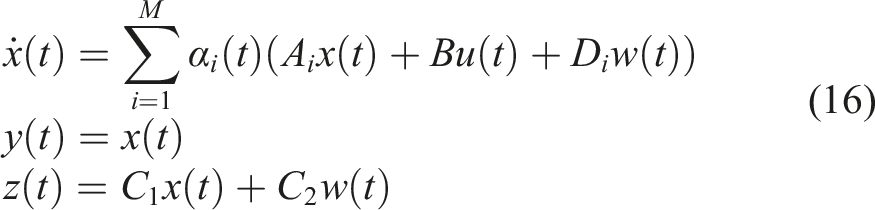
While the aforementioned controllers have shown their ability to improve vehicle performance, they often fail to account for the nonlinear characteristics of semi-active dampers, such as bi-viscous and hysteretic behaviors. To overcome this limitation, the control of semi-active suspensions has been integrated into the Linear Parameter-Varying (LPV) framework (Basargan et al., 2022b; Tian et al., 2022). This framework considers the nonlinear characteristics and allows for online reconfiguration by adjusting the scheduling variables (Basargan et al., 2020, 2021a, 2021b, 2022a). In recent years, there has been growing interest in analyzing and synthesizing sampled-data control strategies for Linear Parameter Varying (LPV) systems (Hooshmandi et al., 2018; 2020b).

H_∞ control has demonstrated effective performance in suspension system control. However, these approaches are primarily designed for continuous-time models, focusing on controllers that operate within a continuous-time framework. In practical implementations, such as in ECUs (Electronic Control Units) within networked systems, challenges arise due to issues like data delays, packet loss, and timing irregularities. In these systems, packet transmission intervals are often irregular. In digital implementations, the sampling period has a significant impact on control system performance, and neglecting this can lead to oscillatory and unstable closed-loop responses. This highlights the importance of aperiodic sampled-data control, which has shown promising results, especially in active suspension systems (Gao et al., 2009; Li et al., 2018, 2020; Na et al., 2019). This raises the possibility of directly designing sampled-data controllers with aperiodic sampling for semi-active suspension systems. Recently, Viadero-Monasterio et al. (2025) introduced a nonlinear sampled-data control approach for MR damper–based semi-active suspensions that avoids Lyapunov–Krasovskii functionals, reducing computational complexity. Their results show that aperiodic sampling can be addressed without the conservatism of conventional delay-dependent methods. Nonetheless, the indicated permissible sampling interval (10–20 ms) demonstrates a level of conservatism in comparison to Lyapunov-based methodologies. Furthermore, the strategy fails to explicitly integrate performance criteria and relies on stability conditions to substantiate its claims of enhanced performance, resulting in a comparison with passive strategies that may not be entirely rigorous.

In this paper, based on time-dependent Lyapunov–Krasovskii functionals and Wirtinger’s inequality, which have been widely discussed in linear sampled-data systems (Barreau et al., 2017), we derive new sufficient conditions for sampled-data LPV systems. As major contribution, the discrepancy between the actual parameters of the semi-active suspension system and their sampled measurements is modeled as uncertainty within this double-layer polytopic framework. Additionally, by utilizing the projection lemma, we establish a new form of stabilization condition. This approach incorporates the sampling period as a parameter in the design process, ensuring that the controller performance accounts for the implementation constraints. This methodology aims to enhance control performance by considering both the LPV framework and the discrete nature of control implementation. To the authors’ knowledge, this topic has not been explored in the design of controllers for semi-active suspension systems, particularly in the context of their nonlinear characteristics.

The mathematical notation used in this paper follows standard conventions. The sets N, Rⁿ, and R^n×m represent the sets of nonnegative integers, real vectors, and real matrices of appropriate dimensions, respectively. Sⁿ and $S_{+}^{n}$ denote the sets of symmetric and symmetric positive-definite matrices. The superscript T indicates matrix transposition, obtained by interchanging rows and columns. For a matrix M ∈ R^n×m with rank(M) = r < n, the symbol M^⊥ denotes its orthogonal complement, which is a matrix whose columns form a basis for the null space of M (satisfying MM^⊥ = 0). For any square matrix X, the Hermitian operator is defined as He(X) = X + X^T. The identity and zero matrices of suitable sizes are denoted by I and 0, respectively, while the symbol ∗ is used to represent symmetric elements within a symmetric block matrix.

2. Description of quarter-vehicle model

This paper focuses on analyzing a quarter-vehicle model as shown in Figure 1. Consider the following equations

\begin{matrix} m_{s} {\ddot{Z}}_{s} (t) = - D_{m r} (t) - k_{s} (Z_{s} (t) - Z_{u} (t)) \\ m_{u} {\ddot{Z}}_{u} (t) = D_{m r} (t) - k_{s} (Z_{u} (t) - Z_{s} (t)) - k_{t} (Z_{u} (t) - Z_{r} (t)) \\ - c_{t} ({\dot{Z}}_{u} (t) - {\dot{Z}}_{r} (t)) \end{matrix}

(1)

Figure 1.

A model depicting a quarter car with a semi active suspension.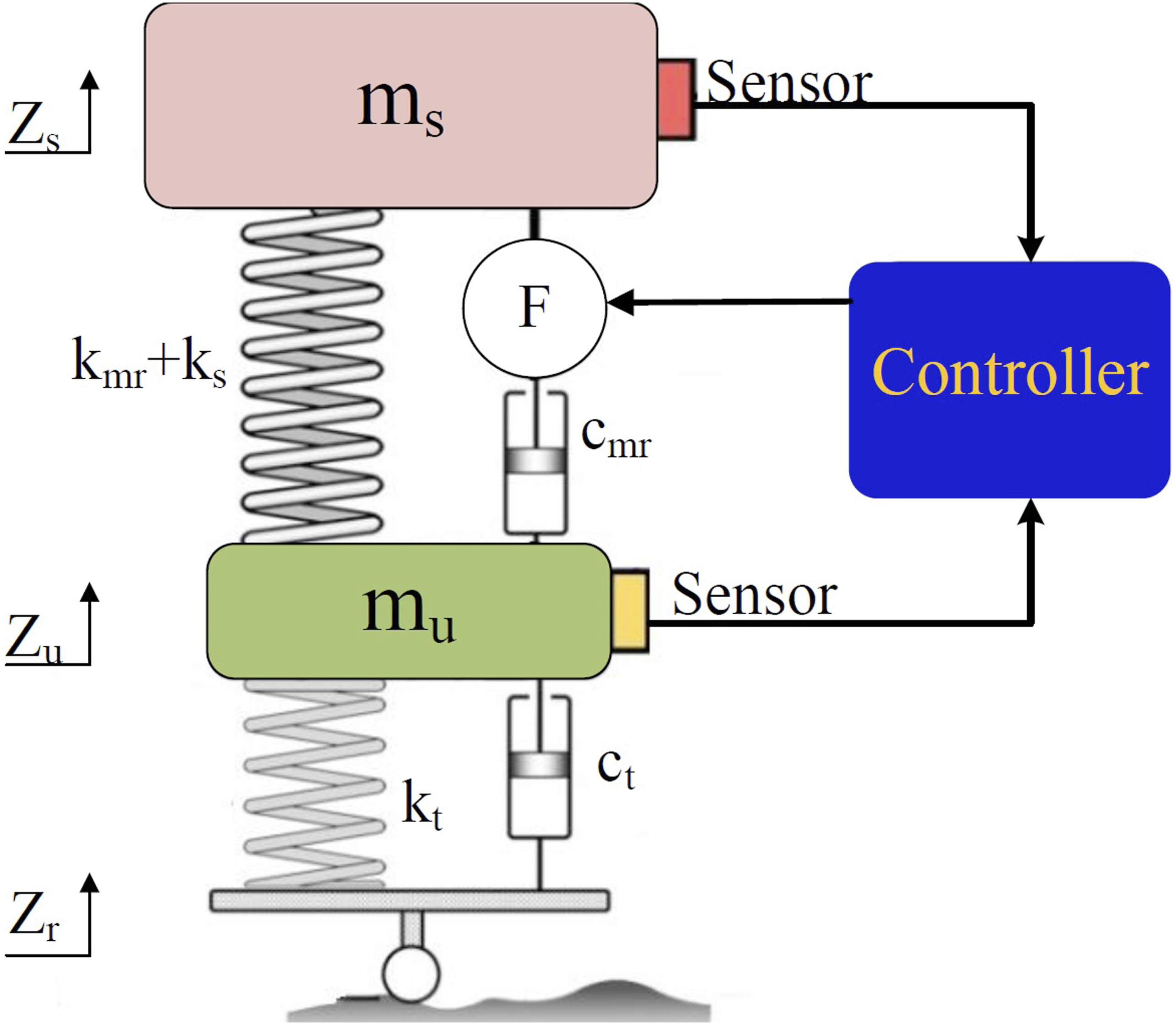

The vehicle body is characterized by the sprung mass m_s, while the wheel setup is represented by the unsprung mass m_u. The semi-active damper force is indicated by D_mr(t), with Z_s and Z_u symbolizing the displacements of the sprung and unsprung masses, respectively. The road displacement input is Z_r, and the stiffness of the suspension system is denoted as k_s. The tire’s flexibility and damping properties are represented by k_t and c_t, respectively.

Consider the following equation for the semi-active damper

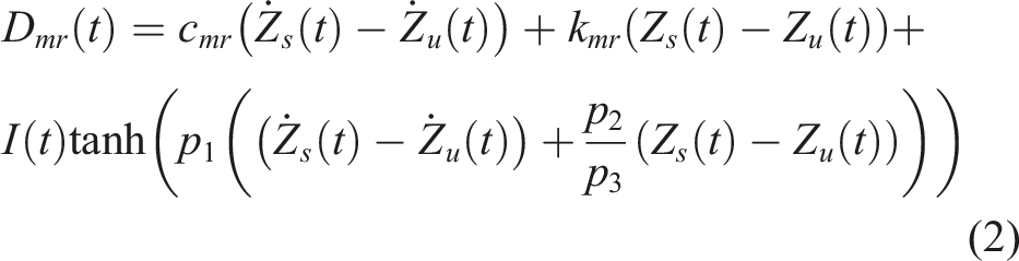
\begin{matrix} D_{m r} (t) = c_{m r} ({\dot{Z}}_{s} (t) - {\dot{Z}}_{u} (t)) + k_{m r} (Z_{s} (t) - Z_{u} (t)) + \\ I (t) \tanh (p_{1} (({\dot{Z}}_{s} (t) - {\dot{Z}}_{u} (t)) + \frac{p_{2}}{p_{3}} (Z_{s} (t) - Z_{u} (t)))) \end{matrix}

(2)

The proposed model in (2) has been validated by comparing it with experimental data and the bi-viscous hysteresis model using a damper force–velocity curve. As shown (Guo et al., 2006), the proposed model matches the experimental results more closely and provides higher accuracy than the bi-viscous hysteresis model. I(t) is the controllable force coefficient which is varying according to the electrical current in the coil (0 ≤ I_min < I ≤ I_max) (Do et al., 2010b). In this context, p₁, p₂, and p₃ are constant parameters, while c_mr and k_mr represent the damping and stiffness parameters, respectively. The semi-active damper model described in (2) is selected for its high fidelity in capturing the bi-viscous and hysteretic behavior of MR fluids. A similar hyperbolic-tangent-based parameterization was recently successfully employed in (Viadero-Monasterio et al., 2024) for the design of robust static output feedback controllers. In this work, however, this model is further embedded into a parameter-varying framework.

Subsequently, we must develop the LPV model. This entails articulating the nonlinear model (1) and (2) within the LPV framework. Let us designate

σ_{1} = \tanh (p_{1} (({\dot{Z}}_{s} (t) - {\dot{Z}}_{u} (t)) + \frac{p_{2}}{p_{3}} (Z_{s} (t) - Z_{u} (t))))

(3)

The quarter car model in state space form can be expressed as follows

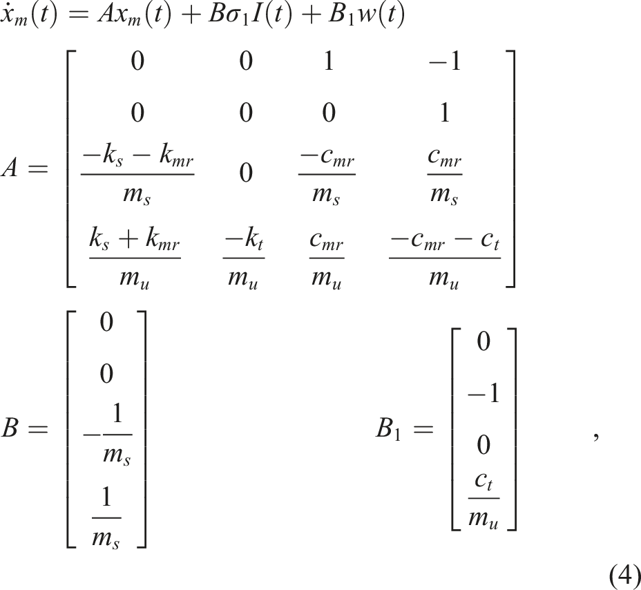
\begin{align} \begin{matrix} {\dot{x}}_{m} (t) = A x_{m} (t) + B σ_{1} I (t) + B_{1} w (t) \\ A = [\begin{matrix} 0 & 0 & 1 & - 1 \\ 0 & 0 & 0 & 1 \\ \frac{- k_{s} - k_{m r}}{m_{s}} & 0 & \frac{- c_{m r}}{m_{s}} & \frac{c_{m r}}{m_{s}} \\ \frac{k_{s} + k_{m r}}{m_{u}} & \frac{- k_{t}}{m_{u}} & \frac{c_{m r}}{m_{u}} & \frac{- c_{m r} - c_{t}}{m_{u}} \end{matrix}] \\ B = [\begin{matrix} 0 \\ 0 \\ - \frac{1}{m_{s}} \\ \frac{1}{m_{s}} \end{matrix}] B_{1} = [\begin{matrix} 0 \\ - 1 \\ 0 \\ \frac{c_{t}}{m_{u}} \end{matrix}], \end{matrix} \end{align}

(4)

The state variables are delineated as follows. x_m1(t) = Z_s(t) − Z_u(t) denotes the suspension displacement, x_m2(t) = Z_u(t) − Z_r(t) signifies the tire displacement, $x_{m 3} (t) = {\dot{Z}}_{s} (t)$ indicates the velocity of the sprung mass, and $x_{m 4} (t) = {\dot{Z}}_{u} (t)$ represents the velocity of the unsprung mass. The disruptive input is represented as $w (t) = {\dot{Z}}_{r} (t)$ . Considering I(t) = u(t) + I_min + I_max/2, the state space representation of the vehicle model is articulated as follows

\begin{align} \begin{matrix} {\dot{x}}_{m} (t) = (A + A_{σ} \frac{σ_{1}}{c x_{m} (t)} c) x_{m} (t) + B σ_{1} I (t) + B_{1} w (t) \\ c = [\begin{matrix} \frac{p_{1} p_{2}}{p_{3}} & 0 & p_{1} & - p_{1} \end{matrix}] \\ A_{σ} = {[\begin{matrix} 0 & 0 & - \frac{I_{\min} + I_{\max}}{m_{s}} & \frac{I_{\min} + I_{\max}}{m_{s}} \end{matrix}]}^{T} \end{matrix} \end{align}

(5)

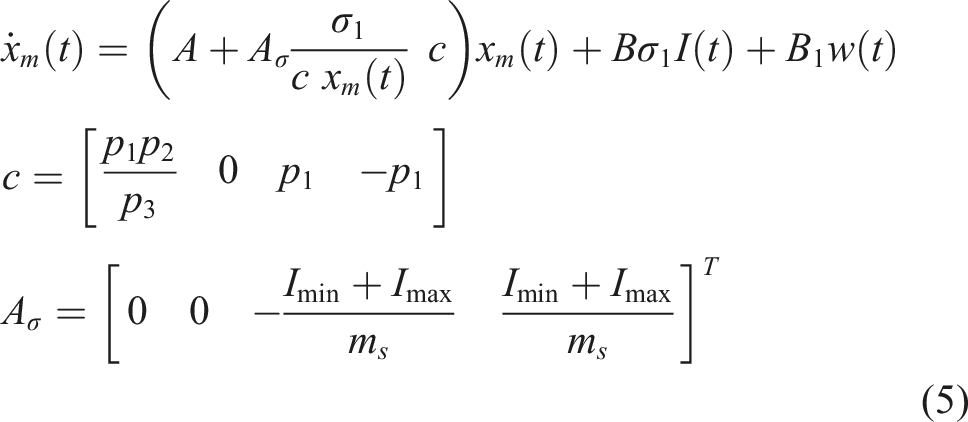
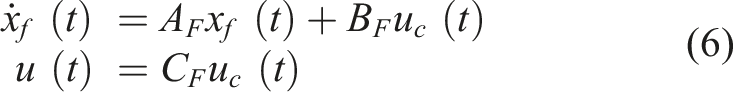
The parameter-dependent control input matrix in (5) presents difficulties for the H_∞ design problem of polytopic systems. To address this issue, a solution can be implemented by incorporating a strictly appropriate filter into (5), thus generating an input matrix that is unaffected by the parameter. Examine the subsequent filter in the system’s input

\begin{align} {\dot{x}}_{f} (t) & = A_{F} x_{f} (t) + B_{F} u_{c} (t) \\ u (t) & = C_{F} u_{c} (t) \end{align}

(6)

Where A_F, B_F, and C_F are constant matrices. By combining equations (5) and (6) and introducing σ₂(t) = σ₁/Cx_m(t), the control-oriented model can be expressed as a system in the LPV form with two parameters, namely σ₁ and σ₂

\dot{x} (t) = A (σ_{1}, σ_{2}) x (t) + B u_{c} (t) + B_{1} w (t)

(7)

Where

x (t) = {[\begin{matrix} x_{m}^{T} (t) & x_{f}^{T} (t) \end{matrix}]}^{T}

\begin{align} \begin{matrix} A (σ_{1}, σ_{2}) = [\begin{matrix} A_{m} + σ_{2} A_{σ} c & σ_{1} B_{m} c \\ 0 & A_{F} \end{matrix}] \\ B = [\begin{matrix} 0 \\ B_{F} \end{matrix}], B_{1} = [\begin{matrix} B_{m} \\ 0 \end{matrix}] \\ σ_{1} (t) = \tanh (c x_{m} (t)) \in [- 1,1] \\ σ_{2} (t) = \frac{\tanh (c x_{m} (t))}{C x_{m} (t)} \in [0,1] \end{matrix} \end{align}

(8)

Remark 1

When the original input matrix depends on the scheduling parameters, direct design of a parameter dependent state feedback controller leads to non convex BMI conditions. By augmenting the system with a stable pre filter, the input matrix of the augmented model becomes constant, which restores convexity and allows the LMI based synthesis. This technique is standard in LPV control, see Sehr and De Oliveira (2017) for a detailed discussion.

Let’s suppose that A_i represents the values of A (σ) at the four corners of the parameter box. The state-space of the polytopic LPV system can be described using the subsequent expressions

\begin{matrix} \dot{x} (t) = A (σ_{1}, σ_{2}) x (t) + B u_{c} (t) + B_{1} w (t) = \\ \sum_{i = 1}^{4} α_{i} (t) (A_{i} x (t) + B u (t) + B_{1} w (t)) \end{matrix}

(9)

Where

\begin{align} α_{1} (t) & = x \times y, α_{2} (t) = (1 - x) \times y \\ α_{3} (t) & = x \times (1 - y), α_{4} (t) = (1 - x) \times (1 - y) \end{align}

(10)

with

x = \frac{σ_{1_\max} - σ_{1} (t)}{σ_{1_\max} - σ_{1_\min}}, y = \frac{σ_{2} (t) - σ_{2_\min}}{σ_{2_\max} - σ_{2_\min}}

(11)

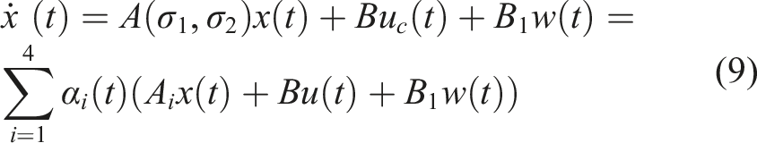
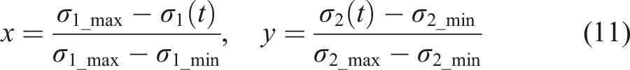
The values α_i are convex coordinates, meeting the conditions 0 ≤ α_i(t) ≤ 1 and $\sum_{i = 1}^{4} α_{i} (t) = 1$ .

In vehicle suspension systems, the control design involves a fundamental trade-off between three conflicting objectives: ride comfort, suspension travel, and road-holding. While minimizing sprung-mass acceleration ${\ddot{Z}}_{s}$ is the primary criterion for enhancing ride comfort, the suspension displacement Z_s − Z_u must be constrained within the mechanical stroke limit Z_max to prevent damaging impacts and events like metal-to-metal contact. Additionally, to ensure road-holding and safety, the dynamic tire load k_t (Z_u − Z_r) must be kept below the total static load (m_s + m_u)g to prevent the wheel from losing contact with the road surface. These objectives are reflected in the choice of controlled outputs z₁(t) and z₂(t), which are defined as follows:

(1) The suspension movement should stay within a predetermined maximum limit imposed by the system

|Z_{s} (t) - Z_{u} (t)| < Z_{\max}

(12)

Where D_max represents the maximum allowable displacement.

(2) Consistent contact between the wheels and the road surface is ensured by maintaining the dynamic tire load below the static tire load

Z_{u} (t) - Z_{r} (t) < (m_{s} (t) + m_{u} (t)) g / k_{t}

(13)

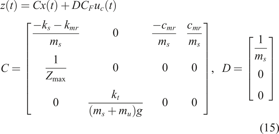
The outputs are defined as

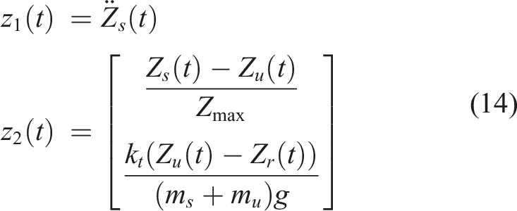
\begin{aligned} z_{1} (t) & = {\ddot{Z}}_{s} (t) \\ z_{2} (t) & = [\begin{matrix} \frac{Z_{s} (t) - Z_{u} (t)}{Z_{\max}} \\ \frac{k_{t} (Z_{u} (t) - Z_{r} (t))}{(m_{s} + m_{u}) g} \end{matrix}] \end{aligned}

(14)

This can be expressed using the following model

\begin{matrix} z (t) = C x (t) + D C_{F} u_{c} (t) \\ C = [\begin{matrix} \frac{- k_{s} - k_{m r}}{m_{s}} & 0 & \frac{- c_{m r}}{m_{s}} & \frac{c_{m r}}{m_{s}} \\ \frac{1}{Z_{\max}} & 0 & 0 & 0 \\ 0 & \frac{k_{t}}{(m_{s} + m_{u}) g} & 0 & 0 \end{matrix}], D = [\begin{matrix} \frac{1}{m_{s}} \\ 0 \\ 0 \end{matrix}] \end{matrix}

(15)

2.1. Problem formulation

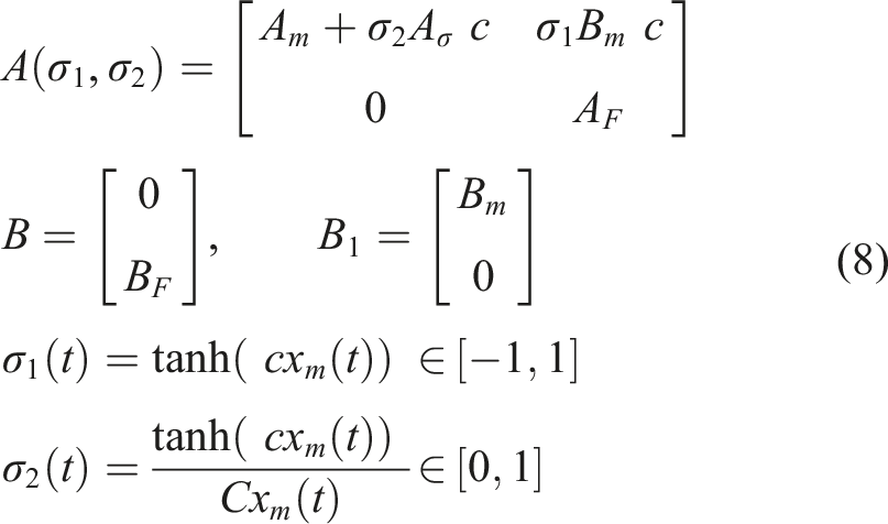
The state-space representation of polytopic LPV systems is characterized by

\begin{matrix} \dot{x} (t) = \sum_{i = 1}^{M} α_{i} (t) (A_{i} x (t) + B u (t) + D_{i} w (t)) \\ y (t) = x (t) \\ z (t) = C_{1} x (t) + C_{2} w (t) \end{matrix}

(16)

Where

x (t) \in R^{n_{x}}

represents the state vector.

u (t) \in R^{n_{u}}

denotes the control input vector.

w (t) \in R^{n_{w}}

signifies the exogenous disturbance vector.

y (t) \in R^{n_{y}}

corresponds to the plant output.

z (t) \in R^{n_{z}}

stands for the vector of controlled outputs. Furthermore, α_i(t) ∈ [0, 1] refers to the time-varying polytopic coordinates that

\sum_{i = 1}^{M} α_{i} (t) = 1, M = 2^{n_{σ}}

(17)

Where σ is the vector of parameters, and n_σ is the count of those parameters. As depicted in Figure 2, the controller output at each sampling interval is determined by the value of the state vector and the LPV parameter. Consequently, the control signal is characterized by being piecewise constant. In this context, the subsequent polytopic state feedback controller is taken into consideration

u (t) = u (t_{k}) = \sum_{i = 1}^{M} α_{i} (t_{k}) K_{i} x (t_{k}),

(18)

Figure 2.

Closed-loop p-LPV sampled-data control system.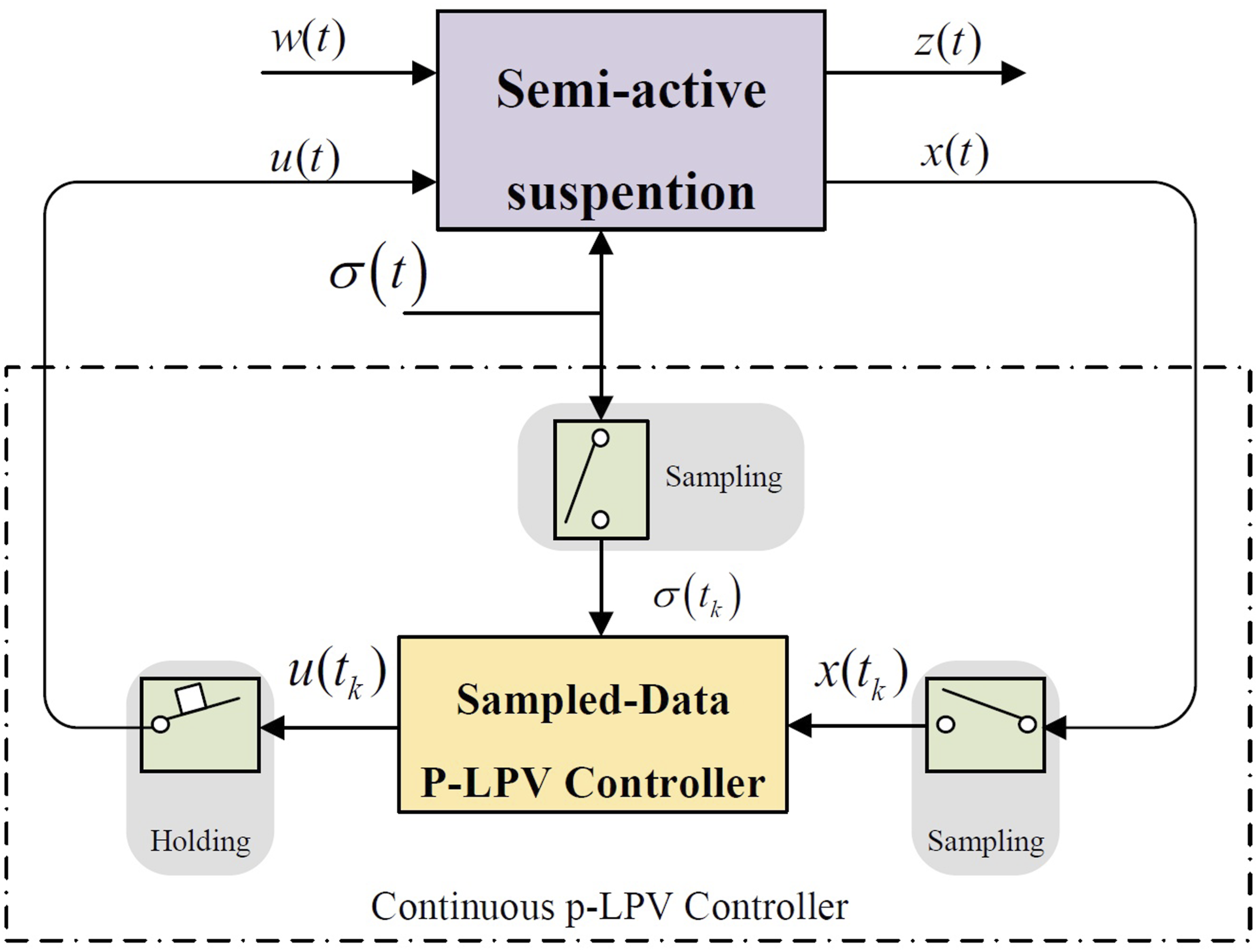

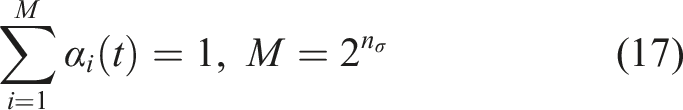
The combined closed-loop interaction between (16) and (18) can be described as follows

\dot{x} (t) = \sum_{i = 1}^{M} α_{i} (t) (A_{i} x (t) + D_{i} w (t)) + \sum_{i = 1}^{M} α_{i} (t_{k}) B K_{i} x (t_{k})

(19)

The delay introduced by the sampler is specified as follows

τ (t) = t - t_{k} f o r t \in [t_{k}, t_{k + 1}), k \in N,

(20)

The maximum sampling time is denoted as

T = S u p (t_{k + 1} - t_{k}) .

(21)

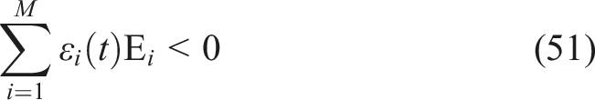
The discrepancy between the actual continuous polytopic parameters of the plant and the discrete piecewise constant polytopic parameters managed by the controller is influenced by the frequency of parameter changes over time and the length of the sampling interval. With considering

{\underset{̲}{α}}_{i} \leq {\dot{α}}_{i} (t) \leq {\bar{α}}_{i}, i = 1, \dots ., M

(22)

By employing (21) and using the mean-value theorem, the following relation is derived

{\underset{̲}{α}}_{i} T \leq α_{i} (t) - α_{i} (t_{k}) \leq {\bar{α}}_{i} T

(23)

Hence, we have

α_{i} (t) = α_{i} (t_{k}) + Δ_{i} (t), {\underset{̲}{α}}_{i} T \leq Δ_{i} (t) \leq {\bar{α}}_{i} T

(24)

Since, $\sum_{i = 1}^{M} α_{i} (t) = 1$ and $\sum_{i = 1}^{M} α_{i} (t_{k}) = 1$ therefore we get $\sum_{i = 1}^{M} Δ_{i} (t) = 0$ . By substituting (24) into (19), we obtain

\dot{x} (t) = \sum_{i = 1}^{M} ε_{i} (t) ((A_{i} + Δ A) x (t) + (D_{i} + Δ D) w (t)) + \sum_{i = 1}^{M} ε_{i} (t) B K_{i} x (t - τ (t))

(25)

Where

\begin{align} Δ A (t) = \sum_{j = 1}^{M - 1} Δ_{j} (t) (A_{j} - A_{M}), \\ Δ D (t) = \sum_{j = 1}^{M - 1} Δ_{j} (t) (D_{j} - D_{M}), \\ ε_{i} (t) = α_{i} (t_{k}) = α_{i} (t - τ (t)) \end{align}

(26)

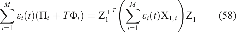
The stability analysis and design issues in equation (19) can be reformulated as the same problem presented in equation (25). This equivalence can be readily verified by employing convex optimization techniques at the vertices of the model. This methodology effectively converts the uncertainty in the controller’s measured parameters into uncertainties within the plant’s parameters, resulting in a closed-loop sampled-data system represented by a double-layer polytopic model, as illustrated in Figure 3.

Figure 3.

A two-layer polytopic LPV framework is used to describe the sampled-data semi-active suspension system.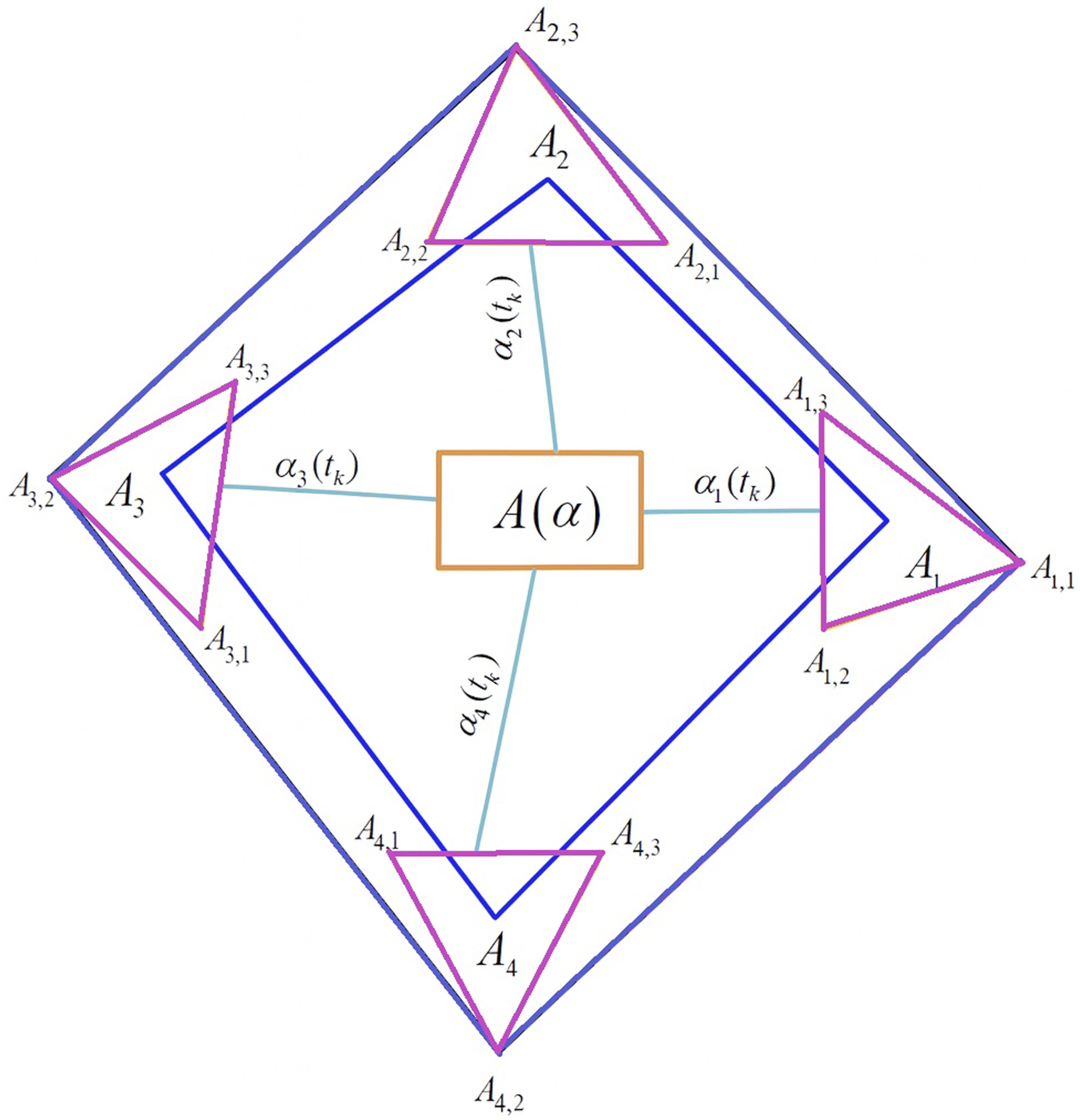

The uncertainties, ΔA and ΔD, are influenced by variations in the sampling period, and their respective bounds play a critical role in determining the controller’s robustness. As these bounds increase, the controller must accommodate a broader spectrum of potential system behaviors, which typically necessitates a more conservative design. While this added conservatism enhances robustness, it may also lead to a compromise in system performance.

Remark 2

The proposed control strategy assumes full state feedback. In commercial series-production vehicles, while suspension displacement x_m1 (via LVDTs) and body acceleration ${\ddot{Z}}_{s}$ (via IMUs) are standard, direct measurement of tire deflection x_m2 and unsprung mass velocity x_m4 is often restricted by sensor costs. However, in practice, this is addressed by implementing a Virtual Sensor or an LPV State Observer. Previous research has shown that the full state vector of a semi-active suspension system can be accurately reconstructed using only the available sensors through LPV observers (Sename et al., 2013) or unscented Kalman filter (Muhammed and Gavrilov I, 2022). Since the separation principle holds for LPV systems, the state feedback gains K_i derived in this work can be integrated with these observers to facilitate real-world implementation.

2.2. Sampled-data stabilization condition

In this section, we aim to establish sufficient conditions for stabilizing the sampled-data p-LPV system using a time-dependent LKF. We will first present some lemmas that are essential for proving these conditions.

Lemma 1

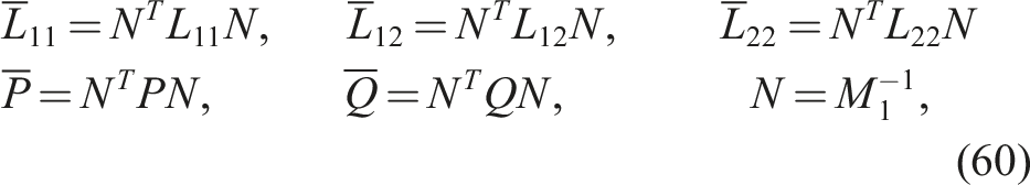
(Apkarian and Gahinet, 1995). For matrices A, B and R >0 with the correct dimensions, the following inequality is satisfied

A B + B^{T} A^{T} \leq A R A^{T} + B^{T} R^{- 1} B .

(27)

Lemma 2

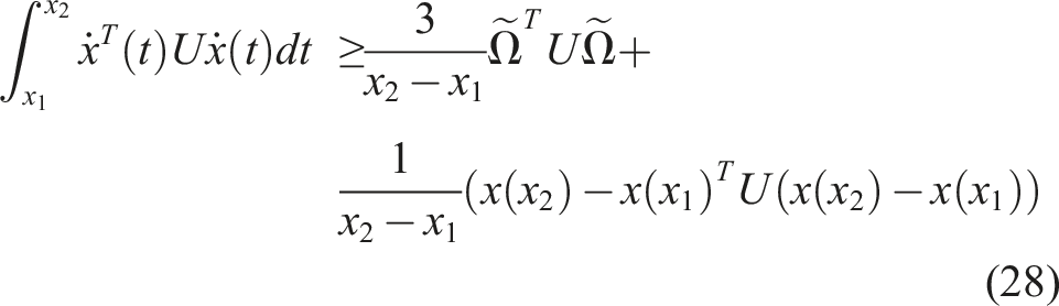
(Basargan et al., 2022b). Considering a given positive definite matrix U, the subsequent inequality is valid for all continuously differentiable functions $x : [x_{1}, x_{2}] \to R^{n}$

\begin{align} \int_{x_{1}}^{x_{2}} {\dot{x}}^{T} (t) U \dot{x} (t) d t & \geq \frac{3}{x_{2} - x_{1}} {\tilde{Ω}}^{T} U \tilde{Ω} + \\ \frac{1}{x_{2} - x_{1}} {(x (x_{2}) - x (x_{1})}^{T} U (x (x_{2}) - x (x_{1})) \end{align}

(28)

Where

\tilde{Ω} = x (x_{2}) + x (x_{1}) - 2 / x_{2} - x_{1} \int_{x_{1}}^{x_{2}} x (t) d t

Lemma 3

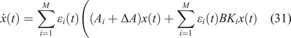
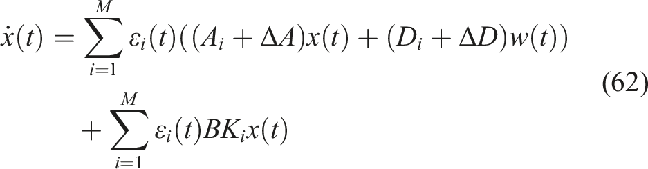
(Hooshmandi et al., 2020a). Given a symmetric matrix X and two matrices F and Z the problem

X + F^{T} M Z + Z^{T} M F < 0

(29)

can be solved for the decision matrix M if and only if

F^{⊥^{T}} X F^{⊥} < 0 Z^{⊥^{T}} X Z^{⊥} < 0

(30)

Where F^⊥ and Z^⊥ show base of the null spaces of F and Z, respectively, FF^⊥ = 0 and ZZ^⊥ = 0.

The following theorem establishes conditions for the asymptotic stabilization of the p-LPV system defined in equation (25) in the absence of disturbances. The model is defined as follows

\dot{x} (t) = \sum_{i = 1}^{M} ε_{i} (t) ((A_{i} + Δ A) x (t) + \sum_{i = 1}^{M} ε_{i} (t) B K_{i} x (t)

(31)

For simplicity, explicit dependence on t is sometimes omitted in the notation.

Theorem 1

Assume there exist matrices $\bar{P} \in S_{+}^{n}$ , $\bar{Q}, {\bar{L}}_{11}, {\bar{L}}_{22} \in S^{n}$ , and matrices ${\bar{E}}_{11, i}, {\bar{E}}_{12, i}, {\bar{E}}_{13, i}, {\bar{E}}_{21, i}, {\bar{E}}_{22, i}, {\bar{E}}_{23, i}, N \in R^{n \times n}$ , and Y_i ∈ R^n×nu with ɛ₁, ɛ₂, ɛ₃ > 0 ensuring that the following LMIs are solvable for i = 1, …, M:

\begin{align} [\begin{matrix} {\bar{L}}_{11} & {\bar{L}}_{12} \\ * & {\bar{L}}_{22} \end{matrix}] > 0 \end{align}

(32a)

\begin{align} [\begin{matrix} \bar{P} + T \bar{Q} & - \bar{Q} \\ * & \bar{Q} \end{matrix}] > 0 \end{align}

(32b)

\begin{align} {\bar{E}}_{i} = [\begin{matrix} (\begin{matrix} T {\bar{L}}_{11} - \\ H e (N) \end{matrix}) & {\bar{O}}_{7, i} & (\begin{matrix} {\bar{O}}_{9, i} + \\ B Y_{i} \end{matrix}) & - T {\bar{L}}_{12} + N \\ * & {\bar{O}}_{8, i} & (\begin{matrix} {\bar{O}}_{2, i} + \\ ε_{1} B Y_{i} \end{matrix}) & (\begin{matrix} - \bar{P} - T \bar{Q} + \\ {\bar{O}}_{3, i} + ε_{1} N \end{matrix}) \\ * & * & (\begin{matrix} T {\bar{L}}_{22} \\ + {\bar{O}}_{4, i} \end{matrix}) & {\bar{O}}_{9, i} + {\bar{O}}_{5, i} \\ * & * & * & T {\bar{L}}_{11} + {\bar{O}}_{6, i} \end{matrix}] < 0 \end{align}

(32c)

\begin{align} {\bar{Ξ}}_{i} = [\begin{matrix} {\bar{O}}_{12, i} & {\bar{O}}_{10, i} & ε_{2} B Y_{i} & ε_{2} N & 0 & 0 \\ * & {\bar{O}}_{11, i} & (\begin{matrix} {\bar{O}}_{2, i} + \\ ε_{3} B Y_{i} \end{matrix}) & (\begin{matrix} - {\bar{P}}_{i} \\ + {\bar{O}}_{3, i} \end{matrix}) & T {\bar{E}}_{11, i} & 3 T {\bar{E}}_{21, i} \\ * & * & (\begin{matrix} T {\bar{L}}_{22} \\ + {\bar{O}}_{4, i} \end{matrix}) & {\bar{O}}_{5, i} & T {\bar{E}}_{12, i} & 3 T {\bar{E}}_{22, i} \\ * & * & * & {\bar{O}}_{6, i} & T {\bar{E}}_{13, i} & 3 T {\bar{E}}_{23, i} \\ * & * & * & * & - T {\bar{L}}_{11} & 0 \\ * & * & * & * & * & - 3 T {\bar{L}}_{11} \end{matrix}] < 0 \end{align}

(32d)

Where

\begin{matrix} {\bar{O}}_{1, i} = - \bar{Q} + H e (- {\bar{E}}_{11, i} - 3 {\bar{E}}_{21, i}) \\ {\bar{O}}_{2, i} = \bar{Q} + {\bar{E}}_{11, i} - {\bar{E}}_{12, i}^{T} - 3 {\bar{E}}_{21, i} - 3 {\bar{E}}_{22, i}^{T} - {\bar{L}}_{12} \\ {\bar{O}}_{3, i} = - {\bar{E}}_{13, i}^{T} + 6 {\bar{E}}_{21, i} - 3 {\bar{E}}_{23, i}^{T}, \\ {\bar{O}}_{4, i} = - \bar{Q} + H e ({\bar{E}}_{12, i} - 3 {\bar{E}}_{22, i}^{T} + {\bar{L}}_{12}) \\ {\bar{O}}_{5, i} = {\bar{E}}_{13, i}^{T} + 6 {\bar{E}}_{22, i} - 3 {\bar{E}}_{23, i}^{T} \\ {\bar{O}}_{6, i} = 6 {\bar{E}}_{23, i} + 6 {\bar{E}}_{23, i}^{T} \\ {\bar{O}}_{7, i} = \bar{P} + T \bar{Q} + (A_{i} + Δ A (t)) N, \\ {\bar{O}}_{8, i} = {\bar{O}}_{1, i} + H e (ε_{1} (A_{i} + Δ A (t)) N) \\ {\bar{O}}_{9, i} = T (- \bar{Q} + {\bar{L}}_{12}), \\ {\bar{O}}_{10, i} = \bar{P} + ε_{2} (A_{i} + Δ A (t)) N \\ {\bar{O}}_{11, i} = {\bar{O}}_{1, i} + H e (ε_{2} (A_{i} + Δ A (t)) N) \\ {\bar{O}}_{12, i} = - ε_{2} H e (N) \end{matrix}

Consequently, the p-LPV controller specified in equation (18), where the vertex gains are determined as K_i = Y_i ⋅ N⁻¹, ensures asymptotic stability of the system described in equation (31) provided that the sampling intervals are sufficiently small, specifically T >0.

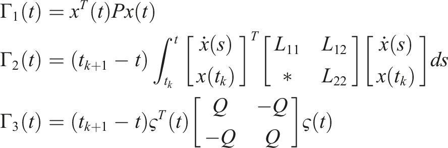
Proof. Take into account the presented LKF for the purpose of stability analysis

Γ (t) = Γ_{1} (t) + Γ_{2} (t, x_{t}, {\dot{x}}_{t}) + Γ_{3} (t, x_{t}),

(33)

\begin{array}{l} \begin{matrix} Γ_{1} (t) = x^{T} (t) P x (t) \\ Γ_{2} (t) = (t_{k + 1} - t) \int_{t_{k}}^{t} {[\begin{matrix} \dot{x} (s) \\ x (t_{k}) \end{matrix}]}^{T} [\begin{matrix} L_{11} & L_{12} \\ * & L_{22} \end{matrix}] [\begin{matrix} \dot{x} (s) \\ x (t_{k}) \end{matrix}] d s \\ Γ_{3} (t) = (t_{k + 1} - t) ς^{T} (t) [\begin{matrix} Q & - Q \\ - Q & Q \end{matrix}] ς (t) \end{matrix} \end{array}

Where

ς^{T} (t) = [x^{T} (t), x^{T} (t_{k})]

In the first step, we establish constraints on the matrices within the LKF to ensure their positivity. Specifically, L₁₁, L₂₂ ∈ Sⁿ must be positive for the integral terms. Combining these with the non-integral terms, we get

Γ_{1} + Γ_{3} = ξ^{T} (t) ([\begin{matrix} P & 0 \\ 0 & 0 \end{matrix}] + (t_{k + 1} - t) [\begin{matrix} Q & - Q \\ * & Q \end{matrix}]) ξ (t),

(34)

As long as P > 0 and the following condition is satisfied

[\begin{matrix} P + T Q & - Q \\ * & Q \end{matrix}] > 0

(35)

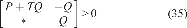
this ensures that there exists a small ɛ such that

ε {‖x (t)‖}^{2} \leq Γ (t) .

(36)

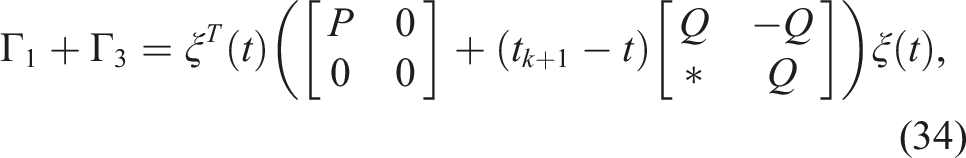
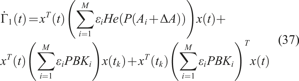
The stability condition is derived from the time derivative of the LKF. The derivative of the Lyapunov function Γ₁(t) along the trajectory of the system is expressed as follows

\begin{matrix} {\dot{Γ}}_{1} (t) = x^{T} (t) (\sum_{i = 1}^{M} ε_{i} H e (P (A_{i} + Δ A))) x (t) + \\ x^{T} (t) (\sum_{i = 1}^{M} ε_{i} P B K_{i}) x (t_{k}) + x^{T} (t_{k}) {(\sum_{i = 1}^{M} ε_{i} P B K_{i})}^{T} x (t) \end{matrix}

(37)

Similarly, the derivative of the Lyapunov function ${\dot{Γ}}_{3} (t, x_{t})$ along the trajectory of the system is given by

\begin{align} \begin{matrix} {\dot{Γ}}_{3} = ς^{T} [\begin{matrix} - Q & Q \\ * & - Q \end{matrix}] ς + \\ (t_{k + 1} - t) ς^{T} (\sum_{i = 1}^{M} ε_{i} [\begin{matrix} H e (Q (A_{i} + Δ A (t))) & * \\ - Q (A_{i} + Δ A (t)) & 0 \end{matrix}]) ς \\ + (t_{k + 1} - t) ς^{T} (\sum_{i = 1}^{M} ε_{i} [\begin{matrix} 0 & Q B K_{i} \\ * & - H e (Q B K_{i}) \end{matrix}]) ς \end{matrix} \end{align}

(38)

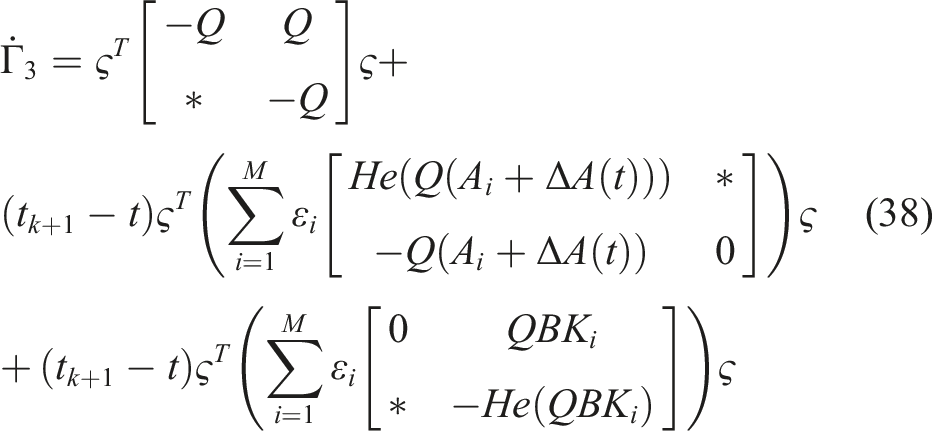
Upon differentiating $Γ_{2} (t, x_{t}, {\dot{x}}_{t})$ , we obtain

\begin{matrix} {\dot{Γ}}_{2} = (t_{k + 1} - t) \{x^{T} (\sum_{i = 1}^{M} ε_{i} 2 {(A_{i} + Δ A (t))}^{T} L_{12}) x (t_{k})\} \\ + (t_{k + 1} - t) \{{\dot{x}}^{T} (t) L_{11} \dot{x} (t) + x^{T} (t_{k}) L_{22} x (t_{k})\} \\ + (t_{k + 1} - t) \{x^{T} (t_{k}) \sum_{i = 1}^{M} ε_{i} 2 {(B K_{i})}^{T} L_{12} x (t_{k})\} \\ - \int_{t_{k}}^{t} {\dot{x}}^{T} (s) L_{11} \dot{x} (s) d s - 2 (x (t) - x (t_{k})) L_{12} x (t_{k}) \\ - τ x^{T} (t_{k}) L_{22} x (t_{k}) \end{matrix}

(39)

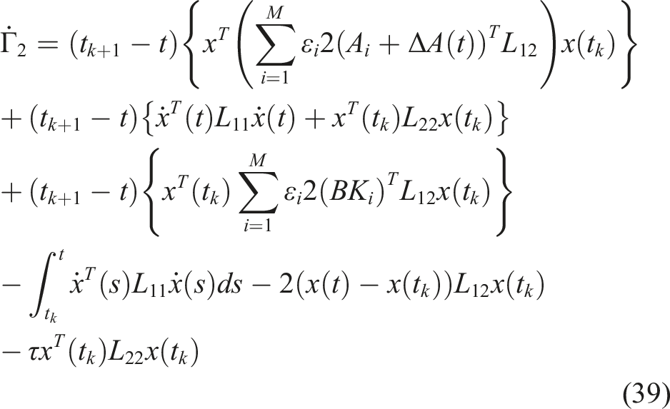
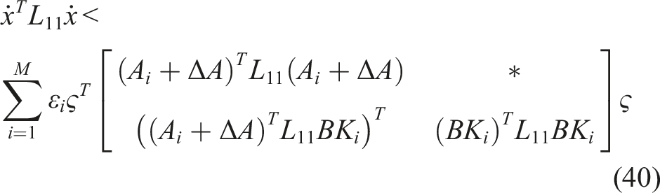
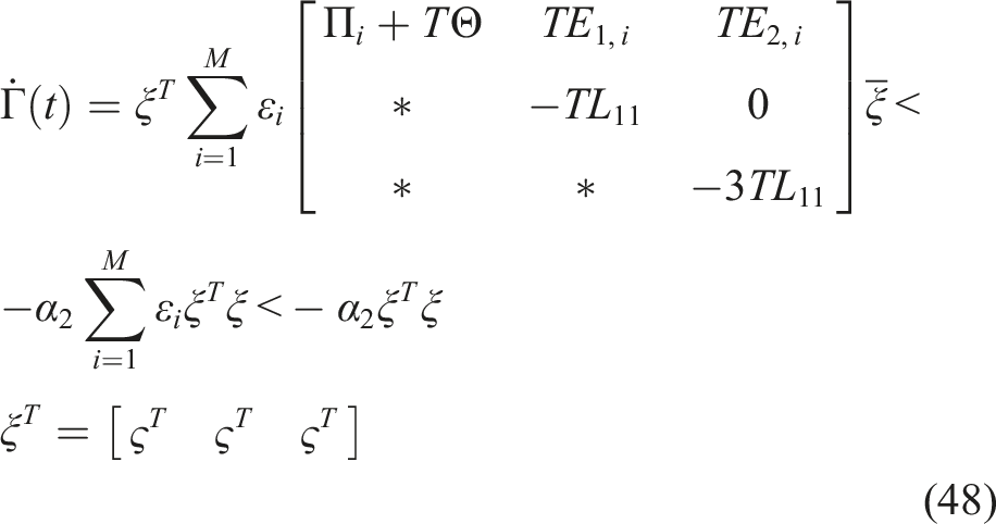
Taking into consideration (31) and Lemma.1, we arrive at the following inequality

\begin{matrix} {\dot{x}}^{T} L_{11} \dot{x} < \\ \sum_{i = 1}^{M} ε_{i} ς^{T} [\begin{matrix} {(A_{i} + Δ A)}^{T} L_{11} (A_{i} + Δ A) & * \\ {({(A_{i} + Δ A)}^{T} L_{11} B K_{i})}^{T} & {(B K_{i})}^{T} L_{11} B K_{i} \end{matrix}] ς \end{matrix}

(40)

By introducing the vector ζ(t) defined as

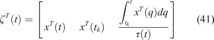
ζ^{T} (t) = [\begin{matrix} x^{T} (t) & x^{T} (t_{k}) & \frac{\int_{t_{k}}^{t} x^{T} (q) d q}{τ (t)} \end{matrix}]

(41)

and utilizing Lemma.2, we arrive at

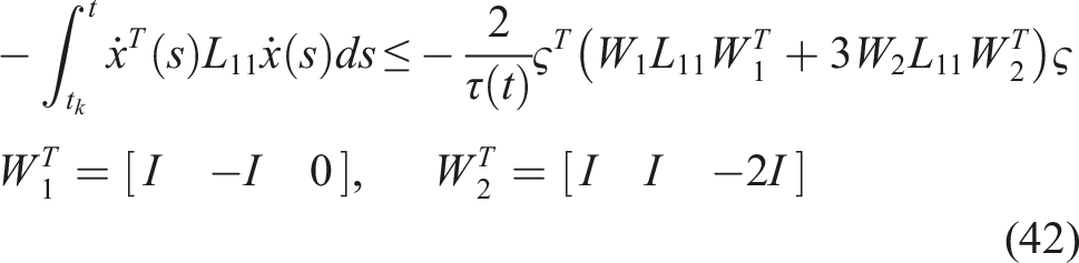
\begin{matrix} - \int_{t_{k}}^{t} {\dot{x}}^{T} (s) L_{11} \dot{x} (s) d s \leq - \frac{2}{τ (t)} ς^{T} (W_{1} L_{11} W_{1}^{T} + 3 W_{2} L_{11} W_{2}^{T}) ς \\ W_{1}^{T} = [\begin{matrix} I & - I & 0 \end{matrix}], W_{2}^{T} = [\begin{matrix} I & I & - 2 I \end{matrix}] \end{matrix}

(42)

By employing Lemma.1, the subsequent inequalities are substituted into equation (42)

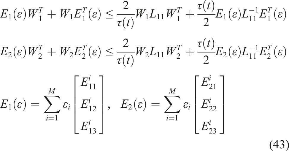
\begin{matrix} E_{1} (ε) W_{1}^{T} + W_{1} E_{1}^{T} (ε) \leq \frac{2}{τ (t)} W_{1} L_{11} W_{1}^{T} + \frac{τ (t)}{2} E_{1} (ε) L_{11}^{- 1} E_{1}^{T} (ε) \\ E_{2} (ε) W_{2}^{T} + W_{2} E_{2}^{T} (ε) \leq \frac{2}{τ (t)} W_{2} L_{11} W_{2}^{T} + \frac{τ (t)}{2} E_{2} (ε) L_{11}^{- 1} E_{2}^{T} (ε) \\ E_{1} (ε) = \sum_{i = 1}^{M} ε_{i} [\begin{matrix} E_{11}^{i} \\ E_{12}^{i} \\ E_{13}^{i} \end{matrix}], E_{2} (ε) = \sum_{i = 1}^{M} ε_{i} [\begin{matrix} E_{21}^{i} \\ E_{22}^{i} \\ E_{23}^{i} \end{matrix}] \end{matrix}

(43)

Therefore $\dot{Γ} (t)$ yields

\begin{matrix} \dot{Γ} (t) = {\dot{Γ}}_{1} (t) + {\dot{Γ}}_{2} (t) + {\dot{Γ}}_{3} (t) \leq \\ ς^{T} (\sum_{i = 1}^{M} ε_{i} Π_{i} + (T_{k} - τ) Φ_{i} + τ Θ_{i}) ς + \\ τ ς^{T} (E_{1} L_{11}^{- 1} E_{1}^{T} + 3 E_{2} L_{11}^{- 1} E_{2}^{T}) ς \end{matrix}

(44)

Where

\begin{matrix} Π_{i}^{11} = H e (P (A_{i} + Δ A (t)) - E_{11, i} - 3 E_{21, i}) - Q \\ Π_{i}^{12} = P B K_{i} + Q + E_{11, i} - E_{12, i}^{T} - 3 E_{21, i} - 3 E_{22, i}^{T} - L_{12} \\ Π_{i}^{13} = - E_{13, i}^{T} + 6 E_{21, i} - 3 E_{23, i}^{T} \\ Π_{i}^{22} = - Q + H e (E_{12, i} - 3 E_{22, i}^{T} + L_{12}) \\ Π_{i}^{23} = E_{13, i}^{T} + 6 E_{22, i} - 3 E_{23, i}^{T}, \\ Π_{i}^{33} = 6 E_{23, i} + 6 E_{23, i}^{T} \\ Φ_{i}^{11} = (A_{i}^{T} + Δ A^{T} (t)) L_{11} (A_{i} + Δ A (t)) + H e (Q (A_{i} + Δ A (t))) \\ Φ_{i}^{12} = (A_{i}^{T} + Δ A^{T} (t)) (- Q + L_{12} + L_{12} B K_{i}) + Q B K_{i} \\ Φ_{i}^{22} = H e ((- Q + L_{12}^{T}) B K_{i}) + L_{22} + K_{i}^{T} B^{T} L_{11} B K_{i} \\ Φ_{i}^{13} = Φ_{i} (2,3) = Φ_{i} (3,3) = 0 \\ Θ = - [\begin{matrix} 0 \\ I \\ 0 \end{matrix}] L_{22} [\begin{matrix} 0 & I & 0 \end{matrix}] \end{matrix}

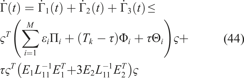
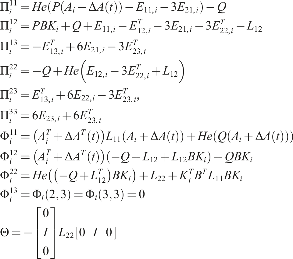
For τ = 0, the following conditions for i = 1, 2, …, M

Π_{i} + T Φ_{i} < 0

(45)

implies

\dot{Γ} (t) = ς^{T} \sum_{i = 1}^{M} ε_{i} (Π_{i} + T Φ_{i}) ς < - α_{1} \sum_{i = 1}^{M} ε_{i} ς^{T} ς < - α_{1} ς^{T} ς

(46)

Also for τ = T

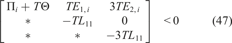
[\begin{matrix} Π_{i} + T Θ & T E_{1, i} & 3 T E_{2, i} \\ * & - T L_{11} & 0 \\ * & * & - 3 T L_{11} \end{matrix}] < 0

(47)

implies

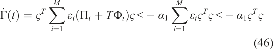
\begin{align} \begin{matrix} \dot{Γ} (t) = ξ^{T} \sum_{i = 1}^{M} ε_{i} [\begin{matrix} Π_{i} + T Θ & T E_{1, i} & T E_{2, i} \\ * & - T L_{11} & 0 \\ * & * & - 3 T L_{11} \end{matrix}] \bar{ξ} < \\ - α_{2} \sum_{i = 1}^{M} ε_{i} ξ^{T} ξ < - α_{2} ξ^{T} ξ \\ ξ^{T} = [\begin{matrix} ς^{T} & ς^{T} & ς^{T} \end{matrix}] \end{matrix} \end{align}

(48)

Given that equation (44) is linear in τ, there exists a small positive scalar α such that $\dot{Γ} (t) < - α |x|$ holds for all time instants $t \in [t_{k}, t_{k + 1})$ . Consequently, when W = 0, the system described by equation (31) is asymptotically stable for sampling intervals shorter than T.

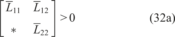
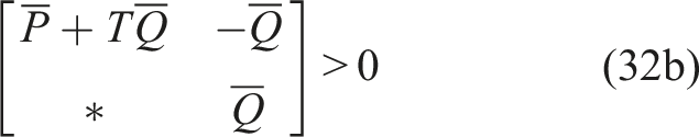
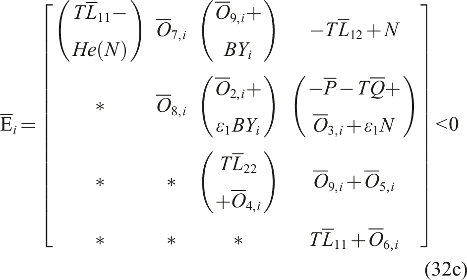
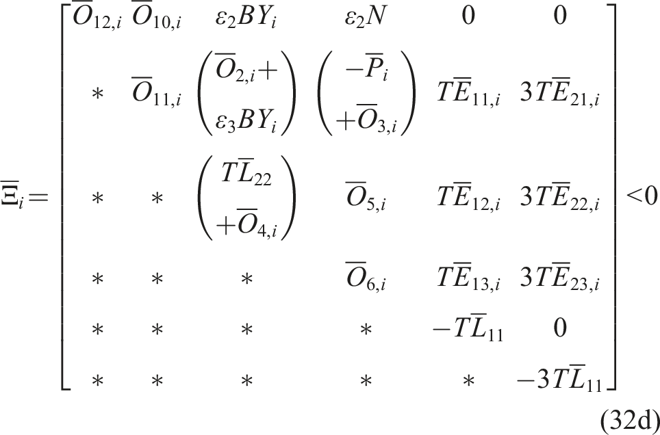
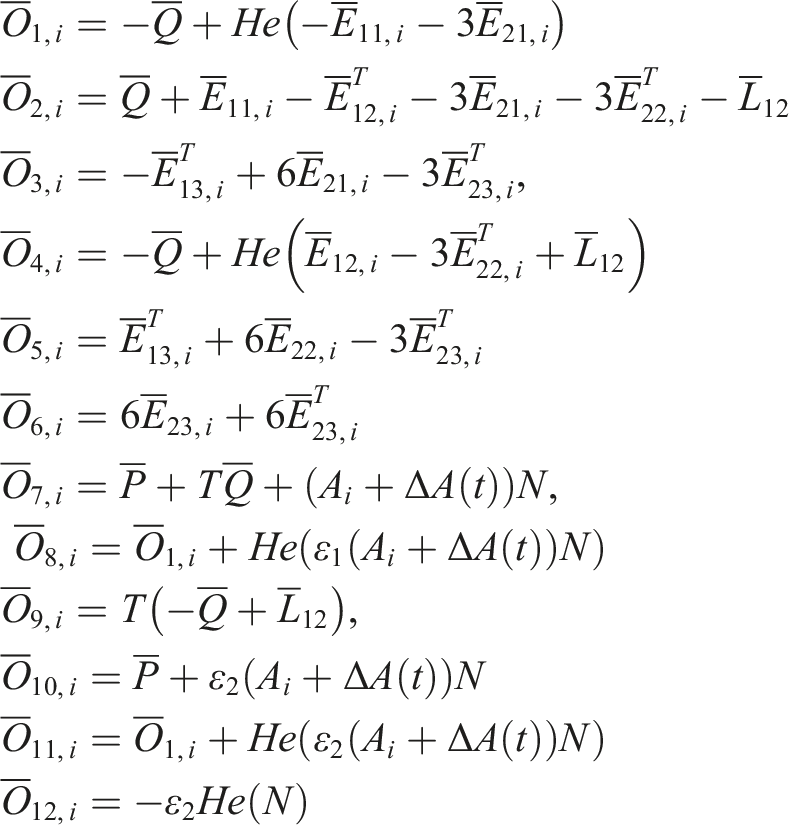
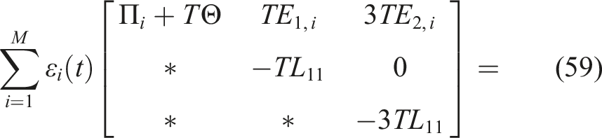
The stability criterion outlined in (45) and (47) are not well-suited for the design of sampled-data p-LPV controllers. This inadequacy arises from the interaction between the system matrix A_i and decision variable matrices, such as P, L₁₁, and Q. To address this issue, these LMI conditions are reformulated using the projection lemma. We utilize Lemma.3 and derive the following conditions

\begin{align} \begin{matrix} E_{i} = [\begin{matrix} O_{12, i} & O_{7, i} & (\begin{matrix} O_{9, i} + \\ M_{1}^{T} B K_{i} \end{matrix}) & - T L_{12} + M_{1}^{T} \\ * & O_{8, i} & (\begin{matrix} O_{2, i} + \\ M_{2}^{T} B K_{i} \end{matrix}) & (\begin{matrix} O_{3, i} - T Q \\ + M_{2}^{T} \end{matrix}) \\ * & * & O_{4, i} & O_{9, i} + O_{5, i} \\ * & * & * & T L_{11} + O_{6, i} \end{matrix}] < 0 \end{matrix} \end{align}

(49)

and

\begin{matrix} Ξ_{i} = [\begin{matrix} O_{13, i} & O_{10, i} & M_{3}^{T} B K_{i} & M_{3}^{T} & 0 & 0 \\ * & O_{11, i} & O_{14, i} & O_{3, i} & T E_{11, i} & 3 T E_{21, i} \\ * & * & O_{4, i} & O_{5, i} & T E_{12, i} & 3 T E_{22, i} \\ * & * & * & O_{6, i} & T E_{13, i} & 3 T E_{23, i} \\ * & * & * & * & - T L_{11} & 0 \\ * & * & * & * & * & - 3 T L_{11} \end{matrix}] < 0 \end{matrix}

(50)

Where

\begin{matrix} O_{1, i} = - Q + H e (- E_{11, i} - 3 E_{21, i}) \\ O_{2, i} = Q + E_{11, i} - E_{12, i}^{T} - 3 E_{21, i} - 3 E_{22, i}^{T} - L_{12} \\ O_{3, i} = - E_{13, i}^{T} + 6 E_{21, i} - 3 E_{23, i}^{T} - P \\ O_{4, i} = - Q + H e (E_{12, i} - 3 E_{22, i}^{T} + L_{12}) + T L_{22} \\ O_{5, i} = E_{13, i}^{T} + 6 E_{22, i} - 3 E_{23, i}^{T}, \\ O_{6, i} = 6 E_{23, i} + 6 E_{23, i}^{T} \\ O_{7, i} = P + T Q + M_{1}^{T} (A_{i} + Δ A (t)), \\ O_{8, i} = O_{1, i} + H e (M_{2}^{T} (A_{i} + Δ A (t))) \\ O_{9, i} = T (- Q + L_{12}) \\ O_{10, i} = P + M_{3}^{T} (A_{i} + Δ A (t)) \\ O_{11, i} = O_{1, i} + H e (M_{4}^{T} (A_{i} + Δ A (t))) \\ O_{12, i} = T L_{11} - H e (M_{1}) \\ O_{13, i} = - H e (M_{3}) \\ O_{14, i} = O_{2, i} + M_{4}^{T} B K_{i} \end{matrix}

When equations (49) and (50) hold for i = 1, …, M, the following condition is satisfied

\sum_{i = 1}^{M} ε_{i} (t) E_{i} < 0

(51)

\sum_{i = 1}^{M} ε_{i} (t) Ξ_{i} < 0

(52)

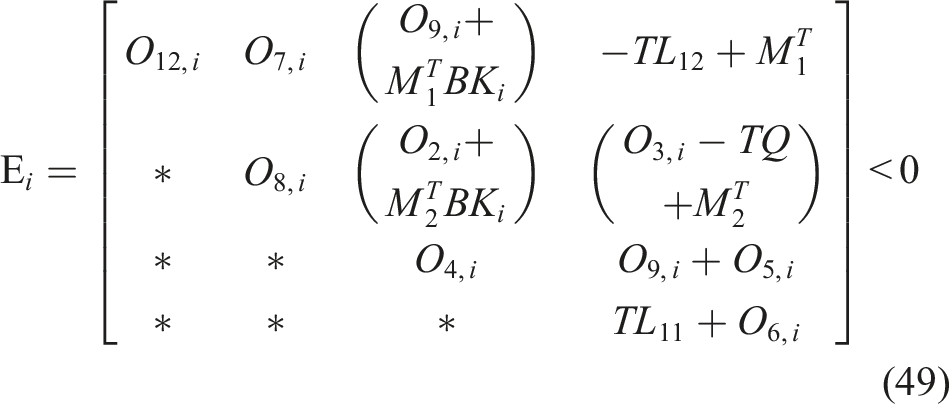
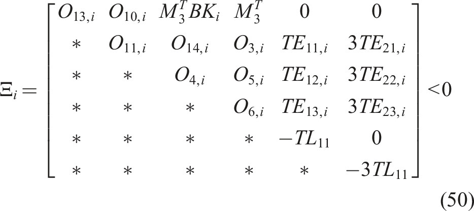
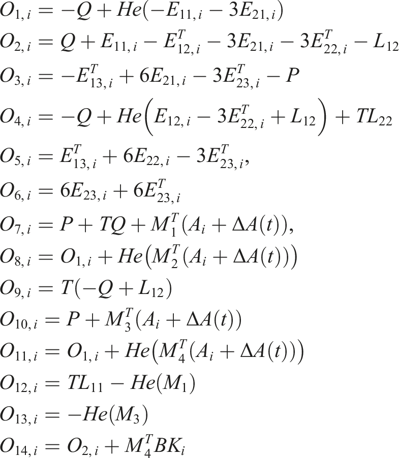
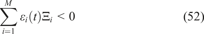
Let’s rewrite equation (51) as

\sum_{i = 1}^{M} ε_{i} (t) X_{1, i} + {F_{1}}^{T} M Z_{1} + Z_{1}^{T} M^{T} F_{1} < 0

(53)

Where

\begin{align} \begin{matrix} X_{1, i} = [\begin{matrix} T L_{11} & P + T Q & O_{7, i} & - T L_{12} \\ * & O_{1, i} & O_{2, i} & - P - T Q + O_{3, i} \\ * & * & T L_{22} + O_{4, i} & O_{7, i} + O_{5, i} \\ * & * & * & T L_{11} + O_{6, i} \end{matrix}] \\ F_{1} = [\begin{matrix} - I & \sum_{i = 1}^{M} ε_{i} (t) (A_{i} + A Δ (t)) & \sum_{i = 1}^{M} ε_{i} (t) B K_{i} & I \end{matrix}] \\ Z_{1} = [\begin{matrix} I & 0 & 0 & 0 \\ 0 & 0 & I & 0 \end{matrix}], M = [\begin{matrix} M_{1} & M_{2} \end{matrix}] \end{matrix} \end{align}

(54)

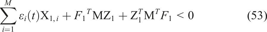
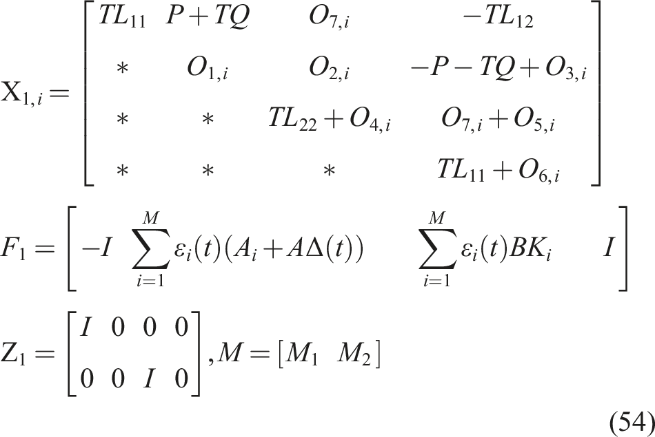
Now, let’s rewrite equation (52) as

\sum_{i = 1}^{M} ε_{i} (t) X_{2, i} + {F_{2}}^{T} \bar{M} Z_{2} + Z_{2}^{T} {\bar{M}}^{T} F_{2} < 0

(55)

Where

\begin{align} \begin{matrix} X_{2, i} = [\begin{matrix} 0 & P & 0 & 0 & 0 & 0 \\ * & O_{1, i} & O_{2, i} & - P + O_{3, i} & T E_{11, i} & 3 T E_{21, i} \\ * & * & T L_{22} + O_{4, i} & O_{5, i} & T E_{12, i} & 3 T E_{22, i} \\ * & * & * & O_{6, i} & T E_{13, i} & 3 T E_{23, i} \\ * & * & * & * & - T L_{11} & 0 \\ * & * & * & * & * & - 3 T L_{11} \end{matrix}] \\ F_{2} = [\begin{matrix} - I & \sum_{i = 1}^{M} ε_{i} (t) (A_{i} + Δ A (t)) & \sum_{i = 1}^{M} ε_{i} (t) B K_{i} & I & 0 & 0 \end{matrix}] \\ Z_{2} = [\begin{matrix} I & 0 & 0 & 0 & 0 & 0 \\ 0 & I & 0 & 0 & 0 & 0 \end{matrix}], \bar{M} = [\begin{matrix} M_{3} & M_{4} \end{matrix}] \end{matrix} \end{align}

(56)

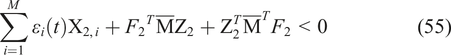
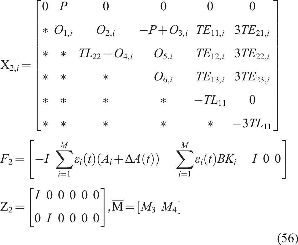
M₁, M₂, M₃, and M₄ are the slack matrix variables. Consider the following null spaces of F₁ and F₂

\begin{align} \begin{matrix} Z_{1}^{⊥} = [\begin{matrix} \sum_{i = 1}^{M} ε_{i} (t) (A_{i} + Δ A (t)) & \sum_{i = 1}^{M} ε_{i} (t) B K_{i} & I \\ I & 0 & 0 \\ 0 & I & 0 \\ 0 & 0 & I \end{matrix}] \\ Z_{2}^{⊥} = [\begin{matrix} \sum_{i = 1}^{M} ε_{i} (t) (A_{i} + Δ A (t)) & \sum_{i = 1}^{M} ε_{i} (t) B K_{i} & I & 0 & 0 \\ I & 0 & 0 & 0 & 0 \\ 0 & I & 0 & 0 & 0 \\ 0 & 0 & I & 0 & 0 \\ 0 & 0 & 0 & I & 0 \\ 0 & 0 & 0 & 0 & I \end{matrix}] \end{matrix} \end{align}

(57)

By applying Lemma.3, we have

\sum_{i = 1}^{M} ε_{i} (t) (Π_{i} + T Φ_{i}) = Z_{1}^{⊥^{T}} (\sum_{i = 1}^{M} ε_{i} (t) X_{1, i}) Z_{1}^{⊥}

(58)

and

\begin{align} \sum_{i = 1}^{M} ε_{i} (t) [\begin{matrix} Π_{i} + T Θ & T E_{1, i} & 3 T E_{2, i} \\ * & - T L_{11} & 0 \\ * & * & - 3 T L_{11} \end{matrix}] = \end{align}

(59)

\begin{array}{l} Z_{2}^{⊥^{T}} (\sum_{i = 1}^{M} ε_{i} (t) X_{2, i}) Z_{2}^{⊥} \end{array}

Therefore, the satisfaction of equation (49) indicates that equation (45) is also feasible. Similarly, if equation (50) is feasible, then equation (47) must be feasible as well.

Applying the congruent transformation diag (N, N) to (35) and

[\begin{matrix} L_{11} & L_{12} \\ * & L_{22} \end{matrix}]

with considering

\begin{matrix} {\bar{L}}_{11} = N^{T} L_{11} N, {\bar{L}}_{12} = N^{T} L_{12} N, {\bar{L}}_{22} = N^{T} L_{22} N \\ \bar{P} = N^{T} P N, \bar{Q} = N^{T} Q N, N = M_{1}^{- 1}, \end{matrix}

(60)

The LMI conditions in equations (32a) and (32b) are obtained. Additionally, by using the congruent transformations diag (N, N, N, N) and diag (N, N, N, N, N, N) to equations (49) and (50), and taking into account

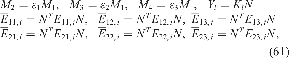
\begin{matrix} M_{2} = ε_{1} M_{1}, M_{3} = ε_{2} M_{1}, M_{4} = ε_{3} M_{1}, Y_{i} = K_{i} N \\ {\bar{E}}_{11, i} = N^{T} E_{11, i} N, {\bar{E}}_{12, i} = N^{T} E_{12, i} N, {\bar{E}}_{13, i} = N^{T} E_{13, i} N \\ {\bar{E}}_{21, i} = N^{T} E_{21, i} N, {\bar{E}}_{22, i} = N^{T} E_{22, i} N, {\bar{E}}_{23, i} = N^{T} E_{23, i} N, \end{matrix}

(61)

the LMI conditions in equations (32c) and (32d) are derived. This concludes the proof.

2.3. H_∞ controller synthesis

In this section, we consider parameter uncertainty in the system described by (25) in the design requirements for a p-LPV controller to achieve H_∞ objectives as a convex optimization problem. This design approach excludes state delays and aims to meet specific H_∞ performance objectives. The model is defined as follows

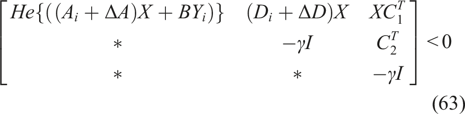
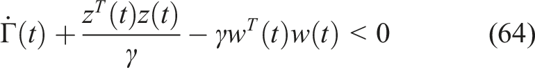
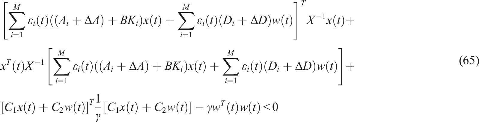
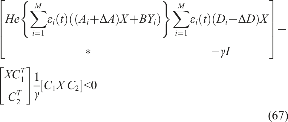
\dot{x} (t) = \sum_{i = 1}^{M} ε_{i} (t) ((A_{i} + Δ A) x (t) + (D_{i} + Δ D) w (t)) + \sum_{i = 1}^{M} ε_{i} (t) B K_{i} x (t)

(62)

The following theorem provides a set of LMIs for calculating the feedback gain matrices K_i. These LMIs ensure that the controller achieves robust performance and stability by handling disturbances and parameter uncertainties effectively. This guarantees that the closed-loop system can withstand external disturbances and parameter variations, maintaining the desired performance level.

Theorem 2

The p-LPV system described in (62) exhibits stability and achieves H_∞ performance, given γ ≥ 0, under zero initial conditions if there exist positive definite matrix functions $X \in S_{+}^{n}$ and matrices $Y_{i} \in R^{n \times n_{u}}$ satisfying the following LMIs for i = 1, 2, …, M

[\begin{matrix} H e \{((A_{i} + Δ A) X + B Y_{i})\} & (D_{i} + Δ D) X & X C_{1}^{T} \\ * & - γ I & C_{2}^{T} \\ * & * & - γ I \end{matrix}] < 0

(63)

subsequently, the control gains K_i can be reconstructed using the formula K_i = Y_iX⁻¹.

Proof. As is well known, the H_∞ stability criterion can be derived from

\dot{Γ} (t) + \frac{z^{T} (t) z (t)}{γ} - γ w^{T} (t) w (t) < 0

(64)

Let Γ(t) = x^T(t)X⁻¹x(t) and substitute equation (62) into equation (64)

\begin{matrix} {[\sum_{i = 1}^{M} ε_{i} (t) ((A_{i} + Δ A) + B K_{i}) x (t) + \sum_{i = 1}^{M} ε_{i} (t) (D_{i} + Δ D) w (t)]}^{T} X^{- 1} x (t) + \\ x^{T} (t) X^{- 1} [\sum_{i = 1}^{M} ε_{i} (t) ((A_{i} + Δ A) + B K_{i}) x (t) + \sum_{i = 1}^{M} ε_{i} (t) (D_{i} + Δ D) w (t)] + \\ {[C_{1} x (t) + C_{2} w (t)]}^{T} \frac{1}{γ} [C_{1} x (t) + C_{2} w (t)] - γ w^{T} (t) w (t) < 0 \end{matrix}

(65)

which leads to

\begin{align} \begin{matrix} [\begin{matrix} H e \{\sum_{i = 1}^{M} ε_{i} (t) X^{- 1} ((A_{i} + Δ A) + B K_{i})\} & \sum_{i = 1}^{M} ε_{i} (t) X^{- 1} (D_{i} + Δ D) \\ * & - γ I \end{matrix}] + \\ [\begin{matrix} C_{1}^{T} \\ C_{2}^{T} \end{matrix}] \frac{1}{γ} [\begin{matrix} C_{1} & C_{2} \end{matrix}] < 0 \end{matrix} \end{align}

(66)

As a result, pre and post multiplying (66), bay diag (X, I) and its transpose yield with considering K_iX = Y_i

\begin{align} \begin{matrix} [\begin{matrix} H e \{\sum_{i = 1}^{M} ε_{i} (t) ((A_{i} + Δ A) X + B Y_{i})\} & \sum_{i = 1}^{M} ε_{i} (t) (D_{i} + Δ D) X \\ * & - γ I \end{matrix}] + \\ [\begin{matrix} X C_{1}^{T} \\ C_{2}^{T} \end{matrix}] \frac{1}{γ} [\begin{matrix} C_{1} X & C_{2} \end{matrix}] < 0 \end{matrix} \end{align}

(67)

By employing the Schur complement, we arrive at the following inequality, which serves as the H_∞ constraint for the closed-loop system when X >0

[\begin{matrix} H e \{\sum_{i = 1}^{M} ε_{i} (t) ((A_{i} + Δ A) X + B Y_{i})\} & \sum_{i = 1}^{M} ε_{i} (t) (D_{i} + Δ D) X & X C_{1}^{T} \\ * & - γ I & C_{2}^{T} \\ * & * & - γ I \end{matrix}] < 0

(68)

Therefore, the H_∞ stability condition given in equation (64) can be ensured by equation (68).

Remark 3

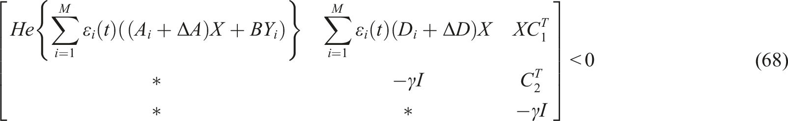
The main aim is to find the feedback gain matrices K_i that meet the H_∞ performance criteria in the context of sampled-data implementation. To achieve this, we considered the conditions from the sampled-data p-LPV controller design in Theorem 1 and the H_∞ p-LPV controller design in Theorem 2. Each theorem independently provides a method for designing a controller; however, by incorporating both approaches, a controller is obtained that possesses the two desired properties: robust H_∞ performance and stability in sampled-data implementations. This combination, assuming N and X are equivalent, yields an LMI-based stabilization condition capable of achieving disturbance rejection while considering sample-and-hold constraints. As a result, the proposed method represents a novel approach to designing H_∞ and sampled-data p-LPV controllers, leading to improved performance with sampled-data controllers.

3. Simulation and experimental results

3.1. Simulation results

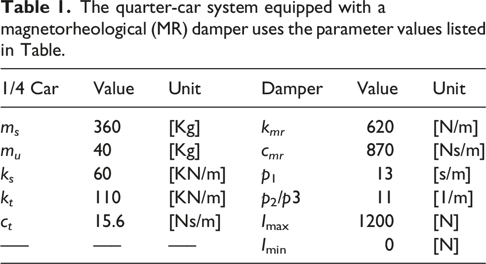
To evaluate the performance of the sampled-data H_∞ p-LPV controller, we designed two different simulation scenarios. The suspension system parameters listed in Table 1 were used in these simulations.

Table 1.

The quarter-car system equipped with a magnetorheological (MR) damper uses the parameter values listed in Table.

1/4 Car	Value	Unit	Damper	Value	Unit
m _s	360	[Kg]	k _mr	620	[N/m]
m _u	40	[Kg]	c _mr	870	[Ns/m]
k _s	60	[KN/m]	p ₁	13	[s/m]
k _t	110	[KN/m]	p₂/p3	11	[1/m]
c _t	15.6	[Ns/m]	I _max	1200	[N]
—–	—–	—–	I _min	0	[N]

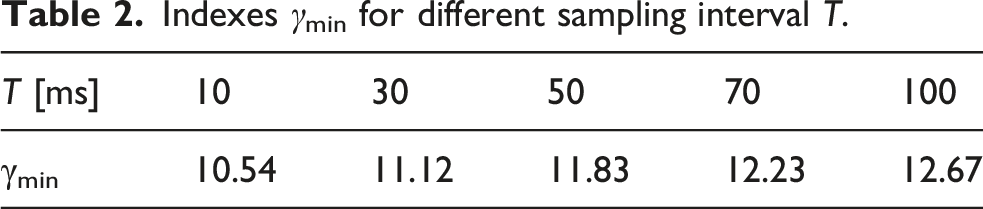
To determine the smallest γ_min with a sampling interval less than T = 100 ms, we solved the LMIs outlined in Theorem 1 and Theorem 2. This was achieved using the YALMIP toolbox (Lofberg, 2004) and the PENBMI solver (Lofberg, 2004). We also included a filter F(s) = 50/s + 50 with a wide bandwidth for the system input. The calculations resulted in a γ_min value of 12.67, and the corresponding controller gain matrices were obtained as follows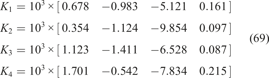

\begin{align} \begin{matrix} K_{1} = 1 0^{3} \times [\begin{matrix} 0.678 & - 0.983 & - 5.121 & 0.161 \end{matrix}] \\ K_{2} = 1 0^{3} \times [\begin{matrix} 0.354 & - 1.124 & - 9.854 & 0.097 \end{matrix}] \\ K_{3} = 1 0^{3} \times [\begin{matrix} 1.123 & - 1.411 & - 6.528 & 0.087 \end{matrix}] \\ K_{4} = 1 0^{3} \times [\begin{matrix} 1.701 & - 0.542 & - 7.834 & 0.215 \end{matrix}] \end{matrix} \end{align}

(69)

To provide a concise reference, we will refer to the proposed controller as ControllerI from this point onward. To clearly demonstrate the impact of increasing the sampling period on the guaranteed performance, we computed γ_min for various sampling intervals T. The results are summarized in Table 2.

Table 2.

Indexes γ_min for different sampling interval T.

T [ms]	10	30	50	70	100
γ_min	10.54	11.12	11.83	12.23	12.67

To evaluate the effectiveness of our new method, we compared the ControllerI with that of ControllerII, which is a continuous H_∞ LPV controller (Apkarian and Gahinet, 1995).

In the first simulation scenario, we model road disturbances as brief but intense events, like large bumps or potholes. The height of these bumps is denoted by S, and their length by l. The road surface is described accordingly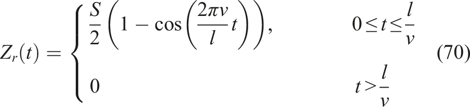

Z_{r} (t) = \{\begin{cases} \frac{S}{2} (1 - \cos (\frac{2 π v}{l} t)), 0 \leq t \leq \frac{l}{v} \\ 0 t > \frac{l}{v} \end{cases}

(70)

These values are set to 50 mm and 6 m, respectively. Also, we consider the vehicle’s forward velocity to be v = 35 km/h.

Remark 4

The road disturbances used in the simulations and experiments are selected such that the required control effort naturally remains within the physical limits of the MR damper. Therefore, the theoretical results in this work are obtained under the assumption that the actuator operates within its admissible range without reaching saturation. A more rigorous mathematical treatment of actuator saturation (e.g., using sector-bounded modeling, anti-windup compensation, or invariant-set constraints) is beyond the scope of this study and is reserved for future research.

The simulation outcomes, utilizing a sampling interval of T = 10 ms, are depicted in Figure 4. This figure displays the speed of the sprung mass, suspension displacement, tire displacement, and control efforts for both active controllersI and II. ControllerII exhibits marginally improved responses than ControllerI. This is mainly because it doesn’t take into account the limitations of the sampling time, which makes it less conservative.

Figure 4.

Responses of the quarter-car suspension model utilizing a maximum sampling interval of T = 10 ms.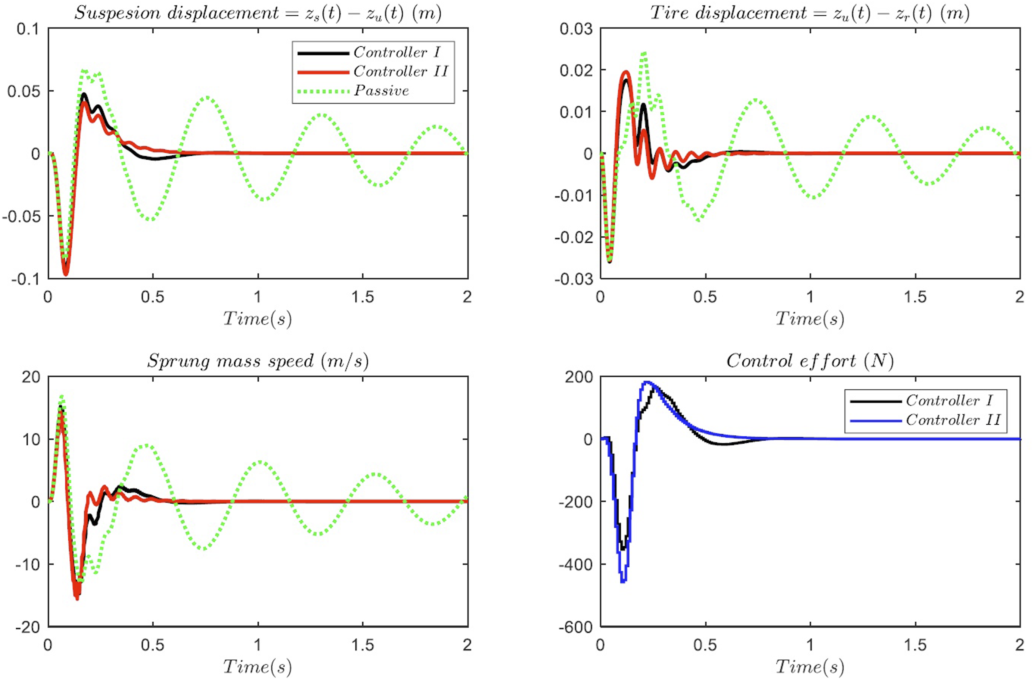

To showcase the advantages of the proposed controller, we increase the sampling period to T = 70 ms and repeat the same simulations. The system responses under both semi-active suspension systems, as well as the passive suspension system for this scenario, are visualized in Figure 5. This figure provides insights into the speed of the sprung mass, suspension displacement, tire displacement, and control effort. It’s worth noting that, with a sampling period of T = 70 ms, controllerII is no longer able to maintain the stability of the suspension system. In contrast, controllerI continues to stabilize the closed-loop system without a noticeable decline in performance.

Figure 5.

Responses of the quarter-car suspension model utilizing a maximum sampling interval of T = 70 ms.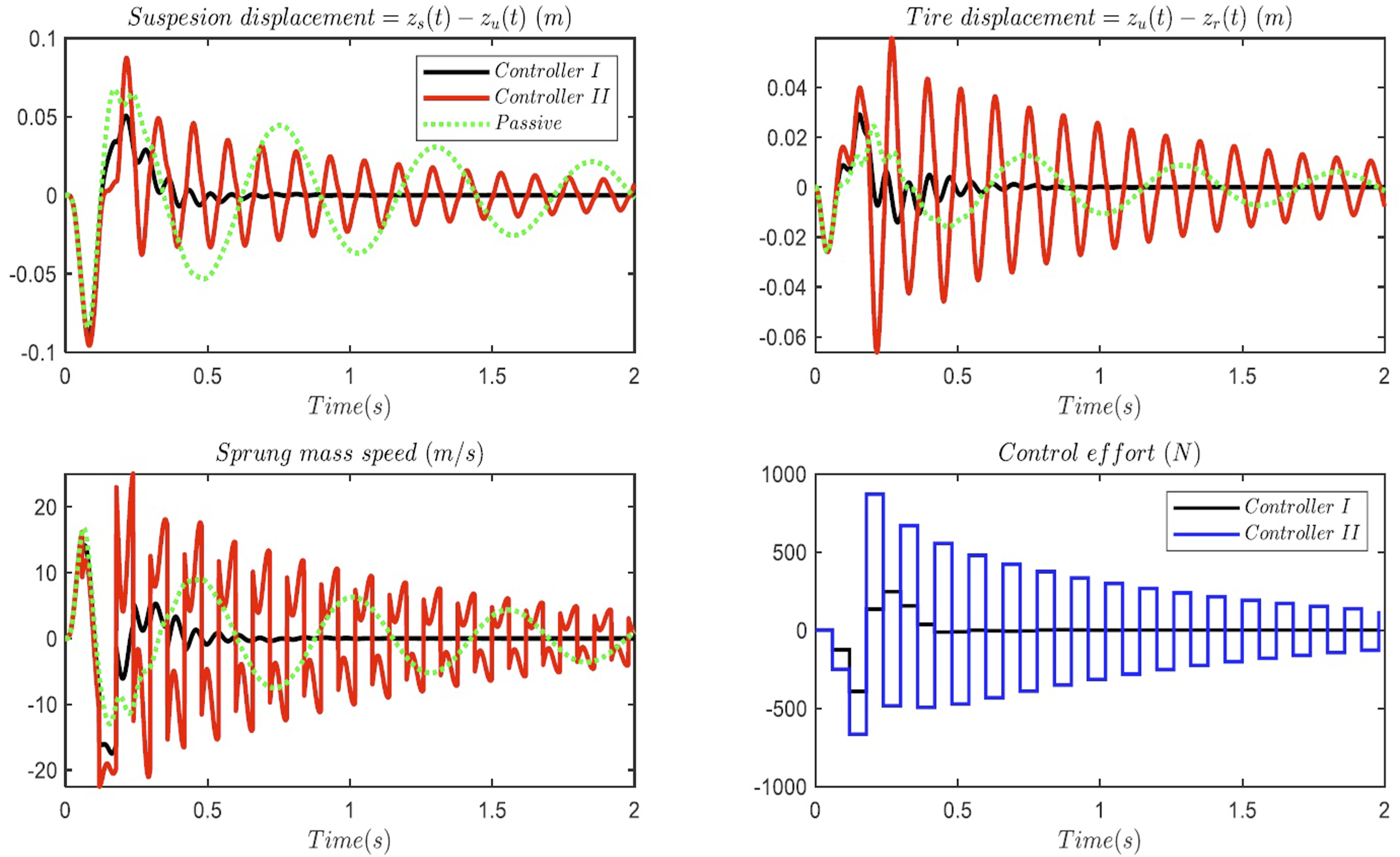

Remark 5

The simulation results highlight the substantial influence of the sampling period on the ride comfort within suspension control systems. Given the limitations of computation and communication time in a car’s ECU, we can infer that the proposed sampled-data H _∞ p-LPV control method effectively bridges the gap between control theory and its practical application in vehicle suspension systems.

In the second simulation scenario, road disturbances are modeled as random vibrations characterized by a specific power spectral density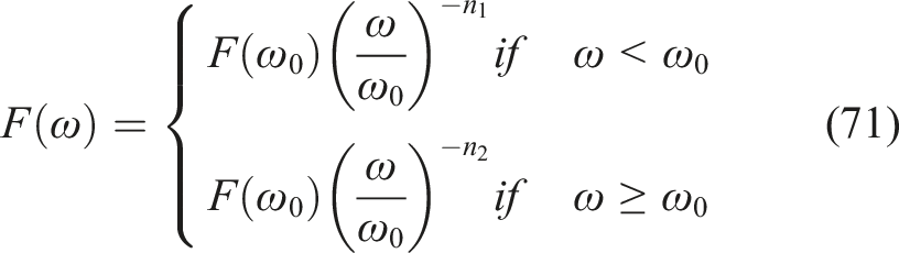

F (ω) = \{\begin{cases} F (ω_{0}) {(\frac{ω}{ω_{0}})}^{- n_{1}} i f ω < ω_{0} \\ F (ω_{0}) {(\frac{ω}{ω_{0}})}^{- n_{2}} i f ω \geq ω_{0} \end{cases}

(71)

Here, ω stands for spatial frequency and ω₀ = 1/2π represents a reference frequency. The parameter

F (ω_{0})

serves as an indicator of road roughness, with n₁ and n₂ being constants associated with road roughness.

Assuming the vehicle travels on a road with a length of L at a speed V₀, the force resulting from road irregularities is represented by the following series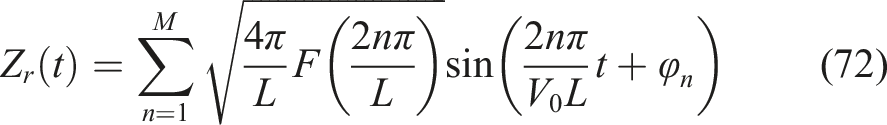

Z_{r} (t) = \sum_{n = 1}^{M} \sqrt{\frac{4 π}{L} F (\frac{2 n π}{L})} \sin (\frac{2 n π}{V_{0} L} t + φ_{n})

(72)

Considered as random variables, the phases φ_n follow a uniform distribution within the interval [0, 2π).

To evaluate the performance of the suspension system, the RMS values of the states are utilized to demonstrate the effectiveness of the proposed control design method. RMS values are closely linked to ride comfort and are commonly employed to quantify the level of acceleration transmitted to the vehicle body. For a very poor quality road (class E, where

F (ω_{0}) = 1024 \times 1 0^{- 6} m^{3}

), the RMS values for sprung mass speed, suspension displacement, and tire displacement are calculated with the parameters n₁ = 2, n₂ = 1.5, L = 100 and M = 200. The horizontal speed is set at V₀ = 20 m/s. The simulation is executed randomly 120 times, and the results are summarized in Table 3 for various sampling times, employing both controllersI and II.

Table 3.

RMS values of sprung mass speed, suspension displacement, and tire displacement for various sampling times.

Quantity	T = 10 ms		T = 60 ms
Quantity	Passive	I, II	Passive	I, II
Sprung mass speed [m/s]
(×10⁻⁵)	38.2	7.19, 6.52	42.1	8.94, 13.7
Suspension displacement [m]
(×10⁻⁶)	28.9	8.24, 5.48	31.5	9.41, 31.4
Tire displacement [m]
(×10⁻³)	1.92	0.29, 0.27	2.11	0.31, 0.66

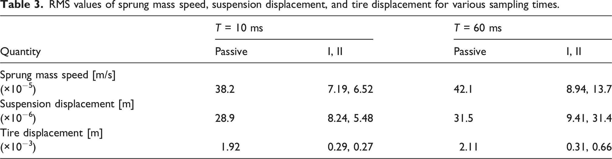
Table.3 shows that both controllers outperform the passive suspension system for various sampling times. The RMS values of sprung mass speed, suspension displacement, and tire displacement are nearly identical for Controller I and Controller II with small sampling times τ = 10 ms. However, with a longer time delay (τ = 60 ms), ControllerI, which accounts for the sampling time, improves ride comfort and meets strict constraints under different road conditions. This improvement is significant when compared to ControllerII, which does not consider the sampling time delay. Taking into account the random vibrations in the road profile as defined in equation (72), Figure 6 depicts the responses of the suspension model with a sampling interval of T = 60, ms.

Figure 6.

Responses of the quarter-car suspension model utilizing a maximum sampling interval of T = 60 ms.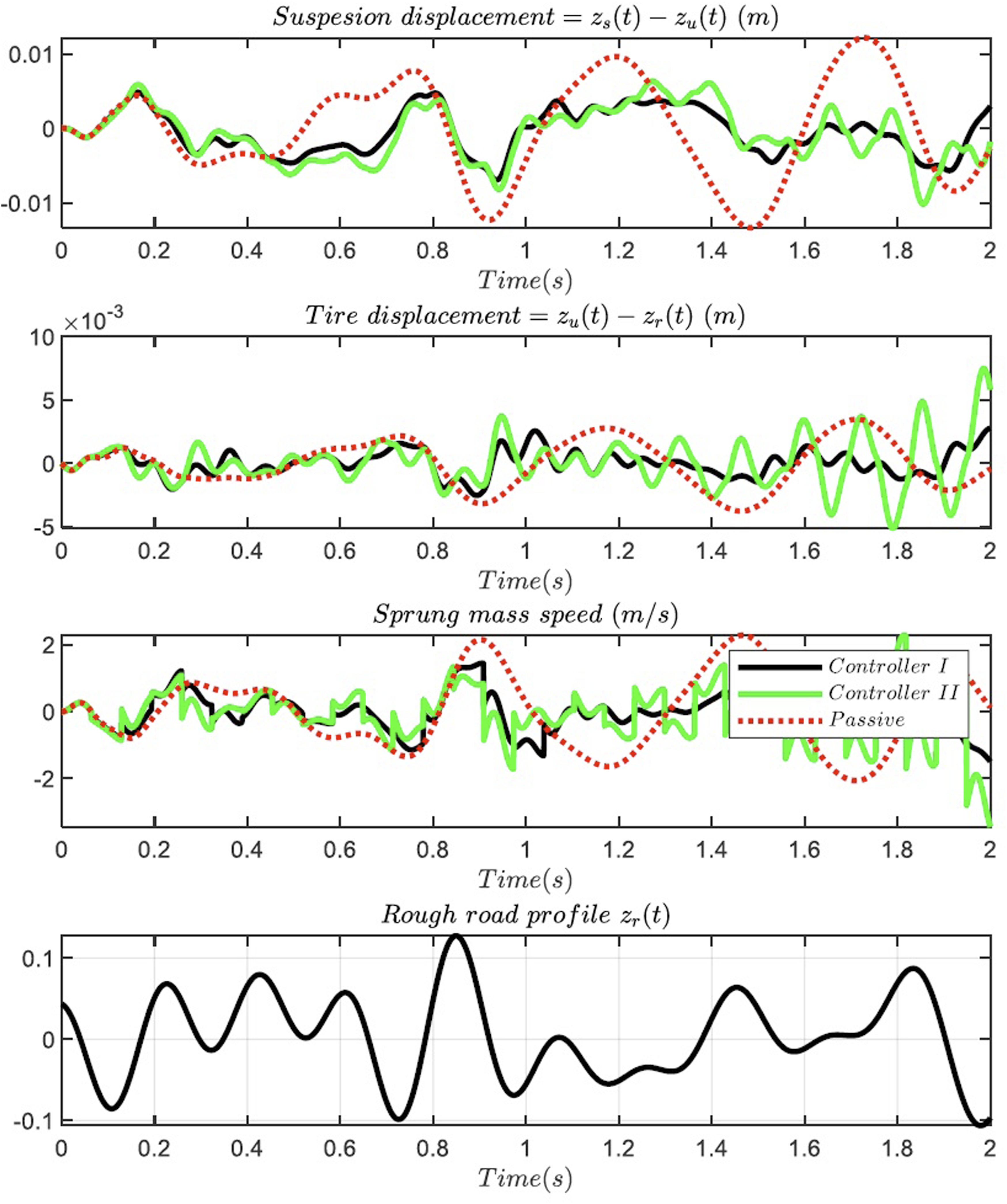

By considering the sampling period, we have demonstrated that, for a 10 ms sampling period, the performance of both is nearly the same. However, for sampling periods of 70 ms and 60 ms, which simulate the worst-case scenarios, the proposed method performs better under these conditions. It is important to note that the computational complexity is not increased, as both controllers are LPV-based and have the same computational complexity. The advantage of the proposed method lies in its ability to handle aperiodic sampling and ensure better performance under worse-case conditions, without a significant increase in computational load.

3.2. Experimental results

To bridge the gap between numerical simulation and practical implementation, a Hardware-in-the-Loop (HiL) real-time validation was conducted. As illustrated in Figure 7, the experimental architecture comprises a Host PC, a Speedgoat Baseline Real-Time Machine, and a high-speed communication link. In this configuration, the quarter-vehicle suspension plant—utilizing the high-fidelity nonlinear model and parameters defined in Table 1 was executed within the MATLAB/Simulink environment on the Host PC. The proposed aperiodic LPV controller was implemented on the Speedgoat real-time hardware, which acts as the industrial-grade engine control unit (ECU). The Speedgoat machine is equipped with a 2 GHz quad-core CPU and operates under a Real-Time Operating System (RTOS) to ensure the deterministic execution of the control law.

Figure 7.

Experimental setup including the Host PC and the Speedgoat baseline real-time machine.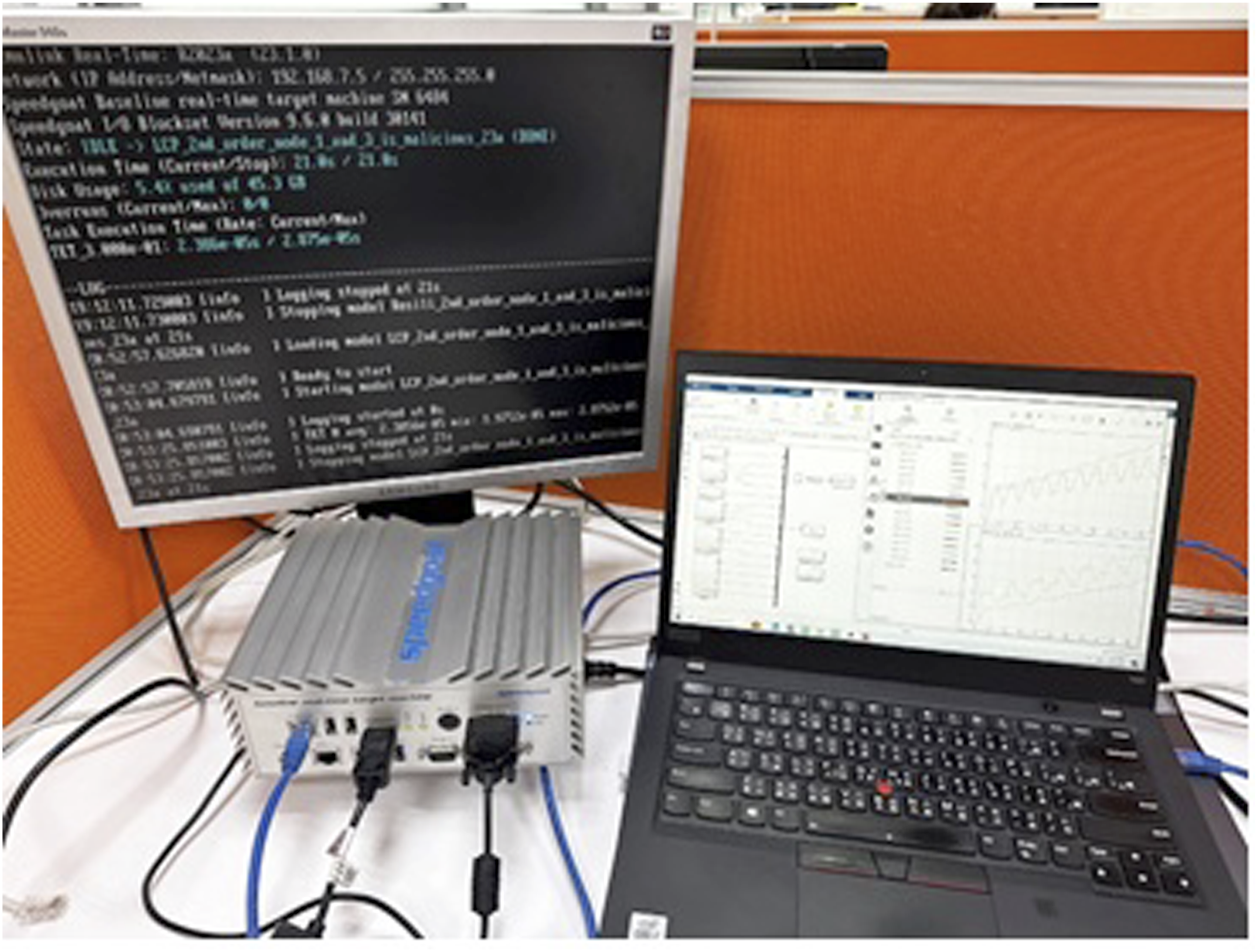

The communication between the virtual plant (Host PC) and the hardware controller (Speedgoat) was established via a low-latency Ethernet link. To realize the aperiodic sampling investigated in the theoretical sections, two factors were utilized: first, the inherent stochastic timing jitter and variable latencies arising from the non-real-time environment of the Host PC and second, an additional random delay introduced into the communication link from the Speedgoat back to the Host PC. Together, these mechanisms simulate the irregular update intervals typical of a networked control system, causing the sampling period in our experiment to vary unpredictably within the range of 10 ms–60 ms.

The trigger logic was implemented such that the Speedgoat controller computes a new control command only upon receiving a fresh measurement packet from the plant. Crucially, the actual elapsed time since the previous update is measured directly on the Speedgoat hardware and is utilized as the real-time sampling period τ(t) within the control law. This HiL validation proves that the proposed LPV gain-scheduling logic is not only computationally feasible for real-time applications but also robust against the non-deterministic timing conditions common in networked automotive systems.

Figure 8 presents the experimental results for the same bump road disturbance used in the first simulation scenario, with sampling intervals varying randomly within the range of 10 ms–60 ms. The responses show that the proposed aperiodic sampled-data H_∞ p-LPV controller maintains closed-loop stability and achieves satisfactory ride comfort, thus validating the theoretical findings under hardware-in-the-loop conditions.

Figure 8.

Experimental results for the sampled-data LPV controller under hardware-in-the-loop with road disturbances and sampling intervals between 10 ms and 60 ms.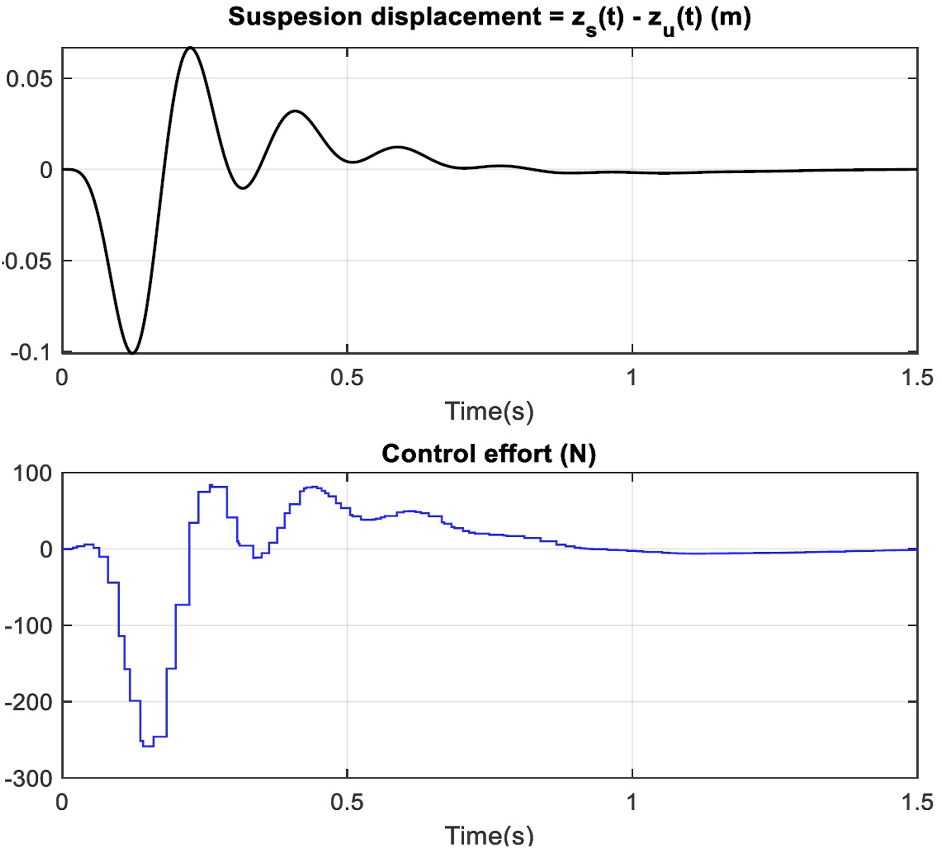

4. Conclusion

This article dealt with the aperiodic sampled-data H_∞ control of semi-active suspension systems by employing a polytopic LPV model. The p-LPV model used for suspension systems supports uncertainties arising from differences between actual and measured parameters. The paper establishes synthesis conditions for stability and H_∞ performance, employing a time-dependent Lyapunov–Krasovskii functional and Wirtinger’s inequality in the form of LMI. This design approach guarantees robust performance, even when dealing with changing sampling periods. The controller design algorithm was verified through numerical simulations, which confirmed the effectiveness of the proposed approach using the quarter-vehicle model. Future research directions may include addressing input saturation to enhance the controller’s adaptation to real-world applications.

Footnotes

ORCID iDs

Kaveh Hooshmandi

Saleh Mobayen

Funding

The authors received no financial support for the research, authorship, and/or publication of this article.

Declaration of conflicting interests

The authors declared no potential conflicts of interest with respect to the research, authorship, and/or publication of this article.

References

Anaya-Martinez

Lozoya-Santos

Tudon-Martinez

, et al. (2020) Control of automotive semi-active mr suspensions for in-wheel electric vehicles. Applied Sciences 10(13): 4522. https://doi.org/10.3390/app10134522

Apkarian

Gahinet

(1995) A convex characterization of gain-scheduled H_∞ controllers. IEEE Transactions on Automatic Control 40(5): 853–864. https://doi.org/10.1109/9.384219

Barreau

Seuret

Gouaisbaut

(2017) Wirtinger-based exponential stability for time-delay systems. IFAC-PapersOnLine 50(1): 11984–11989. https://doi.org/10.1016/j.ifacol.2017.08.1890

Basargan

Mihály

Gáspár

, et al. (2020) Adaptive semi-active suspension and cruise control through lpv technique. Applied Sciences 11(1): 290. https://doi.org/10.3390/app11010290

Basargan

Mihály

Gáspár

, et al. (2021a) Road adaptive semi-active suspension and cruise control through lpv technique. In: 2021 European control conference (ECC), Rotterdam, Netherlands, 29 June 2021–2 July 2021. IEEE, pp. 461–466.

Basargan

Mihály

Gáspár

, et al. (2021b) Road quality information based adaptive semi-active suspension control. Periodica Polytechnica Transportation Engineering 49(3): 210–217. https://doi.org/10.3311/pptr.18577

Basargan

Mihály

Gáspár

, et al. (2022a) An lpv-based online reconfigurable adaptive semi-active suspension control with mr damper. Energies 15(10): 3648. https://doi.org/10.3390/en15103648

Basargan

Mihály

Gáspár

, et al. (2022b) Lpv-fuzzy control approach for road adaptive semi-active suspension system. In: 2022 IEEE Intelligent Vehicles Symposium (IV). IEEE, pp. 779–784.

Ben Hassen

Haddar

Ben Jdidia

, et al. (2023) A modified coupling independent component analysis algorithm applied to a semi-active suspension system. Journal of the Brazilian Society of Mechanical Sciences and Engineering 45(1): 50. https://doi.org/10.1007/s40430-022-03978-x

10.

Ding

Wang

Meng

, et al. (2023) Research on time-delay-dependentH_∞ optimal control of magnetorheological semi-active suspension with response delay. Journal of Vibration and Control 29(5–6): 1447–1458. https://doi.org/10.1177/10775463211064380

11.

Sename

Dugard

(2010a) An lpv control approach for semi-active suspension control with actuator constraints. In: Proceedings of the 2010 American control conference, Baltimore, Maryland, USA, 30 June 2010–2 July 2010. IEEE, pp. 4653–4658.

12.

Sename

Dugard

(2010b) An lpv control approach for semi-active suspension control with actuator constraints. In: Proceedings of the 2010 American control conference, Baltimore, Maryland, USA, 30 June 2010–2 July 2010. IEEE, pp. 4653–4658.

13.

Sename

Dugard

(2012) Lpv modeling and control of semi-active dampers in automotive systems. In: Control of Linear Parameter Varying Systems With Applications. Springer Nature, pp. 381–411.

14.

Gao

Sun

Shi

(2009) Robust sampled-data H_∞ control for vehicle active suspension systems. IEEE Transactions on Control Systems Technology 18(1): 238–245.

15.

Guo

Yang

Pan

(2006) Dynamic modeling of magnetorheological damper behaviors. Journal of Intelligent Material Systems and Structures 17(1): 3–14. https://doi.org/10.1177/1045389x06055860

16.

Hooshmandi

Bayat

Jahed-Motlagh , et al. (2018) Robust sampled-data control of non-linear lpv systems: time-dependent functional approach. IET Control Theory & Applications 12(9): 1318–1331. https://doi.org/10.1049/iet-cta.2017.0980

17.

Hooshmandi

Bayat

Motlagh

J-

, et al. (2020a) Polynomial lpv approach to robust H_∞ control of nonlinear sampled-data systems. International Journal of Control 93(9): 2145–2160. https://doi.org/10.1080/00207179.2018.1547422

18.

Hooshmandi

Bayat

Jahedmotlagh

, et al. (2020b) Guaranteed cost nonlinear sampled-data control: applications to a class of chaotic systems. Nonlinear Dynamics 100: 731–748. https://doi.org/10.1007/s11071-020-05540-7

19.

Zhang

Yan

, et al. (2018) Adaptive event-triggered fuzzy control for uncertain active suspension systems. IEEE Transactions on Cybernetics 49(12): 4388–4397. https://doi.org/10.1109/tcyb.2018.2864776

20.

Xie

Cao

, et al. (2020) Sampled-data asynchronous fuzzy output feedback control for active suspension systems in restricted frequency domain. IEEE/CAA Journal of Automatica Sinica 8(5): 1052–1066. https://doi.org/10.1109/jas.2020.1003306

21.

Lofberg

(2004) Yalmip: a toolbox for modeling and optimization in matlab. In: 2004 IEEE international conference on robotics and automation (IEEE Cat. No. 04CH37508), New Orleans, LA, USA, 02–04 September 2004. IEEE, pp. 284–289.

22.

Moaaz

Ghazaly

(2019) Semi-active suspension system control using skyhook and groundhook controller. International Journal of Advanced Science and Technology 28: 424–433.

23.

Muhammed

Gavrilov

(2022) Unscented kalman-filter to manage the handling-comfort trade-off of quarter-of-vehicle. Transactions of the Institute of Measurement and Control 44(1): 232–244. https://doi.org/10.1177/01423312211031774

24.

Huang

, et al. (2019) Adaptive finite-time fuzzy control of nonlinear active suspension systems with input delay. IEEE Transactions on Cybernetics 50(6): 2639–2650. https://doi.org/10.1109/tcyb.2019.2894724

25.

Pang

Luo

Wang

, et al. (2023) A stability guaranteed nonfragile fault-tolerant control approach for markov-type vehicle active suspension system subject to faults and disturbances. Journal of Vibration and Control 30: 10775463231160807.

26.

Phu

Choi

(2017) A new adaptive hybrid controller for vibration control of a vehicle seat suspension featuring mr damper. Journal of Vibration and Control 23(20): 3392–3413. https://doi.org/10.1177/1077546316629597

27.

Piñón

Favela-Contreras

Félix-Herrán

, et al. (2021) An arx model-based predictive control of a semi-active vehicle suspension to improve passenger comfort and road-holding. In: Actuators, Vol 10, p. 47. MDPI. https://doi.org/10.3390/act10030047

28.

Savaresi

Spelta

(2007) Mixed sky-hook and Add: Approaching the Filtering Limits of a Semi-active Suspension. Journal of Dynamic Systems, Measurement, and Control 129(4): 382.

29.

Savaresi

Bittanti

Montiglio

(2005) Identification of semi-physical and black-box non-linear models: the case of mr-dampers for vehicles control. Automatica 41(1): 113–127. https://doi.org/10.1016/j.automatica.2004.08.012

30.

Sehr

de Oliveira

(2017) Pre-filtering and post-filtering in gain-scheduled output-feedback control. International Journal of Robust and Nonlinear Control 27(16): 3259–3279. https://doi.org/10.1002/rnc.3738

31.

Sename

Gaspar

Bokor

(2013) Robust Control and Linear Parameter Varying Approaches: Application to Vehicle Dynamics. Springer Science & Business Media, Vol. volume 437.

32.

Sharma

Palli

Sharma

, et al. (2021) Ride behaviour of a four-wheel vehicle using h infinity semi-active suspension control under deterministic and random inputs. International Journal of Vehicle Structures & Systems 13(2): 234–237. https://doi.org/10.4273/ijvss.13.2.18

33.

Shen

Golnaraghi

Heppler

(2006) Semi-active vibration control schemes for suspension systems using magnetorheological dampers. Journal of Vibration and Control 12(1): 3–24. https://doi.org/10.1177/1077546306059853

34.

Theunissen

Tota

Gruber

, et al. (2021) Preview-based techniques for vehicle suspension control: a state-of-the-art review. Annual Reviews in Control 51: 206–235. https://doi.org/10.1016/j.arcontrol.2021.03.010

35.

Tian

Yao

Hang

, et al. (2022) A gain-scheduled robust controller for autonomous vehicles path tracking based on lpv system with mpc and h. IEEE Transactions on Vehicular Technology 71(9): 9350–9362. https://doi.org/10.1109/tvt.2022.3176384

36.

Viadero-Monasterio

Boada

, et al. (2022) H_∞ dynamic output feedback control for a networked control active suspension system under actuator faults. Mechanical Systems and Signal Processing 162: 108050. https://doi.org/10.1016/j.ymssp.2021.108050

37.

Viadero-Monasterio

Meléndez-Useros

Jiménez-Salas

, et al. (2024) Robust static output feedback control of a semi-active vehicle suspension based on magnetorheological dampers. Applied Sciences 14(22): 10336. https://doi.org/10.3390/app142210336

38.

Viadero-Monasterio

Meléndez-Useros

Jiménez-Salas

, et al. (2025) Avoiding lyapunov-krasovskii functionals: simple nonlinear sampled–data control of a semi-active suspension with magnetorheological dampers. Machines 13(6): 512. https://doi.org/10.3390/machines13060512

39.

Wang

Liu

Ding

, et al. (2022) Switching control of semi-active suspension based on road profile estimation. Vehicle System Dynamics 60(6): 1972–1992. https://doi.org/10.1080/00423114.2021.1889621

40.

Zhao

Gao

(2010) Vibration control of seat suspension using hinf reliable control. Journal of Vibration and Control 16(12): 1859–1879.

Aperiodic sampled-data control for semi-active suspension systems using a two-layer polytopic LPV model with H ∞ performance

Abstract

Keywords

1. Introduction

2. Description of quarter-vehicle model

2.1. Problem formulation

2.2. Sampled-data stabilization condition

2.3. H∞ controller synthesis

3. Simulation and experimental results

3.1. Simulation results

3.2. Experimental results

4. Conclusion

Footnotes

ORCID iDs

Funding

Declaration of conflicting interests

References

2.3. H_∞ controller synthesis