Fast wheelset wear-stage recognition based on multi-domain entropy features and an attention-enhanced lightweight 1D-CNN

Abstract

This study proposes an intelligent diagnostic framework for high-accuracy, low-latency monitoring of heavy-haul railway wheelset wear under limited computational resources. The framework combines Variational Mode Decomposition (VMD)-based signal decomposition, multi-domain entropy features, and a lightweight attention-based classifier. The Grey Wolf Optimizer (GWO) is used offline to determine the key VMD parameters, which are then fixed for narrowband decomposition of wheel–rail contact acoustic signals during online diagnosis. Adaptive Time-Domain Discrete Entropy (ATDE) and Frequency-Domain Entropy (FDE) are extracted from each modal component to characterize dynamic complexity and energy distribution, thereby enhancing feature robustness and class separability. A One-Dimensional Convolutional Neural Network (1D-CNN) with an attention mechanism then reweights the features and identifies the wear stage. In the four-stage wheelset wear task, the method achieves 99.88% test accuracy and 99.713% mean accuracy over ten independent runs. Compared with time–frequency image-based deep models, the classifier reduces forward inference time by about 99.74% and uses only 13,848 parameters. These results demonstrate improved computational efficiency without sacrificing accuracy, supporting real-time deployment in resource-constrained conditions. Validation on the HUST bearing dataset further suggests its applicability to different mechanical diagnostic tasks.

Keywords

wheelset wear fault diagnosis vibration signals multi-domain entropy features deep attention network

1. Introduction

Wheelsets are critical load-bearing and guiding components in rail vehicles, and their condition directly affects operational safety. Long-term wheel–rail interaction may initiate fatigue cracks at the contact interface and lead to severe failures (Qi et al., 2024; Zhang et al., 2025). Current maintenance relies mainly on offline inspection and periodic checks, limiting real-time awareness and early warning. Online monitoring and intelligent diagnosis are therefore needed for in-service safety assurance and predictive maintenance (Zhao et al., 2024).

Existing online inspection techniques follow two main routes: non-acoustic and acoustic. Non-acoustic approaches include laser ultrasonics (Montinaro et al., 2019), axle-box acceleration analysis (Xu et al., 2023), machine vision (Ye et al., 2022), infrared thermography (Firlik et al., 2023), and alternating current field measurement (ACFM) (Nicholson and Davis, 2012). They can be effective in specific settings. However, maintaining high sensitivity and real-time performance in complex operating environments remains challenging. By contrast, acoustic emission (AE) is highly sensitive to dynamic damage and is easy to deploy, which supports continuous in-service monitoring (Kocur et al., 2024). Prior work also links acoustic features to crack evolution in a quantitative manner (Tehranchi et al., 2011). Optimizing the processing window length, bandwidth, and feature extraction strategy can further improve damage identification (Liu et al., 2026; Shen, 2022). Recent studies improve diagnostic performance by fusing multi-source signals (Song et al., 2018) or adopting deep learning models, such as a long short-term memory (LSTM) and visual geometry group (VGG) fusion network (Tang et al., 2025) and improved CNNs. Recent deep learning–based fault diagnosis studies have further focused on interpretable modeling, prior knowledge embedding, multimodal fusion, and noise robustness. For example, the Interpretable and Differentiable STFT cross-machine dual-driven adaptation Network (IDSN) embeds a differentiable STFT layer into the network, allowing time–frequency transform parameters to be adaptively adjusted by gradient descent and enhancing time–frequency interpretability in cross-machine diagnosis (He et al., 2023). The Multi-Wavelet Kernel Convolution Neural Network (MWKCNN) constructs multi-wavelet kernel convolutional layers to introduce signal-processing priors, such as continuous wavelet transform, into feature extraction, thereby improving the capture of impact-related fault features (Jiang et al., 2023). For missing sensors or abnormal data, multimodal imputation and fusion frameworks improve diagnostic reliability through data reconstruction, unified representation learning, and CNN-based classification (Zhang et al., 2025). Multi-sensor and multi-scale attention networks further integrate time-domain, frequency-domain, and cross-sensor information to enhance fault identification under noisy conditions (Ji et al., 2025). However, performance gains often come with higher computational cost and model complexity, limiting real-time deployment under resource constraints. Both one-dimensional sequences and two-dimensional images can serve as classification inputs (Zhang et al., 2023). Yuan et al. (2025) showed that frequency-domain and time–frequency images can improve recognition accuracy and noise robustness. One-dimensional inputs are simpler and usually converge faster with higher inference efficiency, but may be less accurate and robust under strong noise or changing operating conditions (Wang et al., 2025). Two-dimensional inputs require higher-dimensional representations and typically increase parameters, memory use, and inference latency (Lv et al., 2025). Thus, achieving robust, accurate, and low-latency classification under real operating conditions remains an open challenge.

Computational and real-time constraints have increased interest in lightweight modeling and prior-guided feature design. These designs aim to improve diagnostic accuracy while keeping conclusions verifiable. Multi-sensor fusion with lightweight architectures can help balance accuracy and efficiency (Xu et al., 2025). Knowledge distillation offers a similar trade-off (Gong et al., 2023). Signal-processing priors can also be integrated into learning models. This integration reduces computational cost. It can also improve the physical interpretation of features and the traceability of results. Interpretable multiplicative convolutional networks provide one example (Chen et al., 2025). Entropy is increasingly used in this context. It quantifies signal complexity and uncertainty from a nonlinear perspective. It therefore links classical feature engineering to lightweight models. Approximate entropy (Dou et al., 2023), sample entropy (Bai et al., 2024), and permutation entropy (Noman et al., 2024) are widely used. These entropy features can characterize evolving dynamics without high-dimensional inputs. As a result, they offer discriminative yet computation-friendly state representations. This property supports low-dimensional, deployable features for real-time diagnosis in resource-constrained settings.

Nevertheless, entropy-based acoustic diagnosis depends strongly on preprocessing, especially stable modal decomposition. EMD and its variants are widely used for nonstationary signals, but their IMF numbers may vary across samples and they are susceptible to mode mixing and end effects (Li et al., 2017). VMD estimates finite-bandwidth modes under variational constraints and yields a specified number of components, making it more suitable for fixed-size entropy feature matrices. This study therefore proposes a wheelset wear diagnosis framework combining GWO-VMD, multi-domain entropy, and a lightweight attention network. GWO determines the VMD parameters offline, and fixed parameters are then used online for decomposition, entropy extraction, and classification. The contributions are: (1) offline GWO-based optimization of VMD parameters to reduce manual tuning; (2) fusion of ATDE and FDE into a low-dimensional representation of time-domain complexity and frequency-domain energy distribution; and (3) a CBAM-enhanced 1D-CNN for accurate classification under limited computational budgets. In the four-stage task, the method achieves 99.88% accuracy with a model size of tens of kilobytes. The remaining sections describe the method, wheel–rail experiment, HUST validation, and conclusions.

2. Methodology

2.1. Variational Mode Decomposition and parameter optimization

VMD decomposes a signal into finite-bandwidth modes with strong time–frequency concentration. Given a modal number K, it yields the same number of components for different samples, enabling mode-wise ATDE/FDE calculation and fixed-size feature matrices. Since the decomposition quality of VMD is sensitive to the modal number K and the bandwidth penalty factor α (Li et al., 2020), GWO is employed to optimize K and α using the minimum post-decomposition modal entropy as the objective function. (Wang et al., 2025):

H = - \sum_{i = 1}^{N} p (i) \ln (p (i))

(1)

Here, p(i) is the probability distribution of the normalized modal amplitude, and N is the signal length. K is searched from 1 to 20, and α from 0 to 5000. The optimized parameters are used to obtain modal components for feature construction and wear-stage recognition. GWO is performed only offline to determine global K and α, which are fixed for all subsequent samples.

2.2. Multi-domain entropy theory

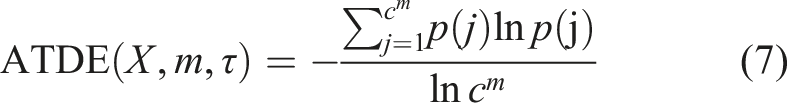
Wheel–rail contact acoustic signals are nonstationary in both time and frequency domains. Crack initiation, spalling, and local adhesion cause transient impacts and amplitude irregularities, whereas wear evolution changes bandwidth, energy migration, and high-frequency components. Therefore, ATDE and FDE are extracted from the IMF components and concatenated along the input-channel dimension. ATDE describes modal time-domain complexity, while FDE describes frequency-domain energy distribution, providing complementary information on temporal evolution and spectral variation. As shown in Figure 1(a), multi-domain entropy features are calculated after GWO-VMD decomposition and then organized as channel-wise concatenated feature inputs for the classifier.

Figure 1.

The detailed framework proposed for wheel–rail wear condition diagnosis.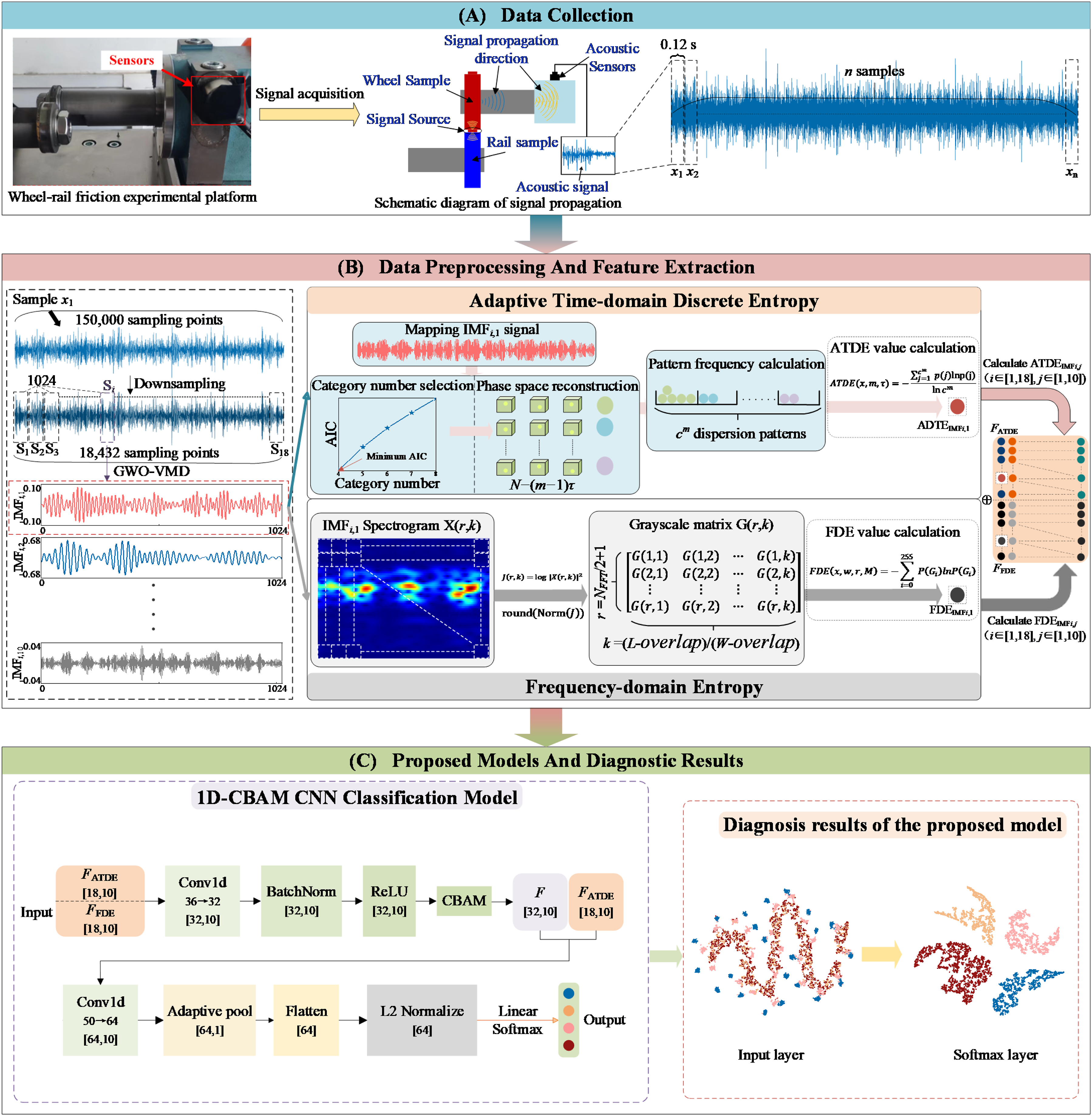

(1) Adaptive Time-domain Discrete Entropy (ATDE)

ATDE is the time-domain part of the multi-domain entropy features. It aims to avoid subjective choices of the discrete class number required by conventional discrete entropy and to improve the robustness of time-domain complexity features (Li et al., 2025). The computation is as follows:

Step 1: Given the input time-series signal $x = {x_{i}}_{i = 1}^{N}$ , compute the mean μ_x, standard deviation σ_x, kurtosis k_x and skewness s_x.

Skewness (X) = \frac{1}{N} \sum_{i = 1}^{n} [{(\frac{x_{i} - μ}{σ})}^{3}]

(2)

Use the skewness s_x to determine the mapping. If │s_x│>1, use the logarithmic transform y_i = log(x_i – min(x)+1), followed by normalization to [0,1]. Otherwise, map the samples via the Gaussian cumulative distribution function (CDF), y_i = Ф(x_i | μ_x, σ_x), and then perform linear normalization.

Step 2: Following Rostaghi and Azami (2016), set the search space of the class number to [c_min, c_max] = [4,8]. For each candidate class number c, compute the log-likelihood function of y.

\log L = \sum_{j = 1}^{c} n_{j} \log (\frac{n_{j}}{N})

(3)

Here, n_j denotes the number of samples in bin j, and L is the maximum likelihood. The Akaike information criterion (AIC) is computed as

AIC (c) = 2 c - 2 \log L

(4)

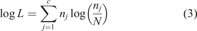
We choose the optimal c that yields the minimum AIC. This choice balances model complexity and fit quality, and it adaptively determines the discretization granularity.

Step 3: With the optimal c, discretize the mapped signal into a symbolic sequence:

z_{i} = round (y_{i} \cdot c + 0.5)

(5)

A discrete symbolic sequence of length N is obtained. We then use the embedding dimension m and delay τ to form candidate patterns. The number of all possible patterns is c^m, which defines the pattern space of length-m symbol sequences.

Step 4: A sliding window is applied to the symbolic sequence. The occurrence count of each pattern yields n=(n₁, n₂, …, n_c^m). The pattern probability distribution is then computed as

p_{j} = \frac{n_{j}}{N - (m - 1) τ}, j = 1, 2, . . ., c^{m}

(6)

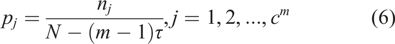
We only retain patterns with nonzero probability for subsequent computation to reduce bias from sparse sampling.

Step 5: We compute the discrete entropy and then normalize it to remove scale differences caused by the choice of c and m:

ATDE (X, m, τ) = - \frac{\sum_{j = 1}^{c^{m}} p (j) \ln p (j)}{\ln c^{m}}

(7)

(2) Frequency-Domain Entropy (FDE)

FDE characterizes the complexity of energy distribution in the joint time–frequency domain. It leverages time–frequency variation and grayscale mapping to describe the spectral energy distribution and its changes over time. The computation is as follows:

Step 1: For the signal $x = {x_{i}}_{i = 1}^{N}$ , the short-time Fourier transform (STFT) is computed to obtain the matrix X:

X (r, k) = \sum_{n = 0}^{M - 1} x (n) w (n - r) e^{- j \frac{2 π k n}{M}}

(8)

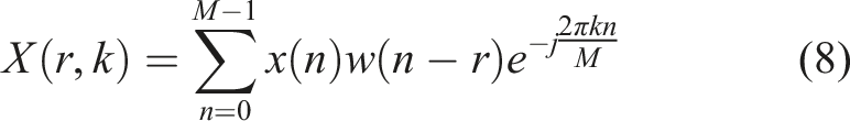
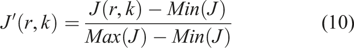
In this formulation, X(r,k) is the STFT coefficient at time index r and frequency bin k, and w(n-r) denotes the window function. r is the time shift, and M is the FFT length. We use a window length of 128, 50% overlap, and 256-point FFT. The resulting spectrogram-based comparison map J is given by:

J (r, k) = \log | X (r, k) ∣^{2}

(9)

Here, │X(r, k)│denotes the magnitude of X(r, k).

Step 2: The log-spectral matrix J is normalized to yield Jʹ:

J^{'} (r, k) = \frac{J (r, k) - Min (J)}{Max (J) - Min (J)}

(10)

Here, Min(J) is the minimum value of the matrix J, and Max(J) is the maximum value of J.

Step 3: The normalized matrix Jʹ is mapped to a grayscale matrix G:

G (r, k) = r o u n d (J^{'} (r, k) \times 255)

(11)

Step 4: We estimate the probability of each gray level in G. The frequency entropy is then computed as

F D E (x, w, r, M) = - \sum_{i = 0}^{255} P (G_{i}) I n P (G_{i})

(12)

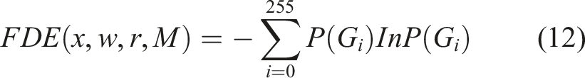
Here, P(G_i) is the occurrence probability of gray level G_i in G.

2.3. 1D-CBAM CNN classification model

CNNs extract hierarchical features through local receptive fields and weight sharing (Sudarshan et al., 2024). In one-dimensional modeling, convolution kernels capture local patterns and progressively transform low-level cues into discriminative representations.

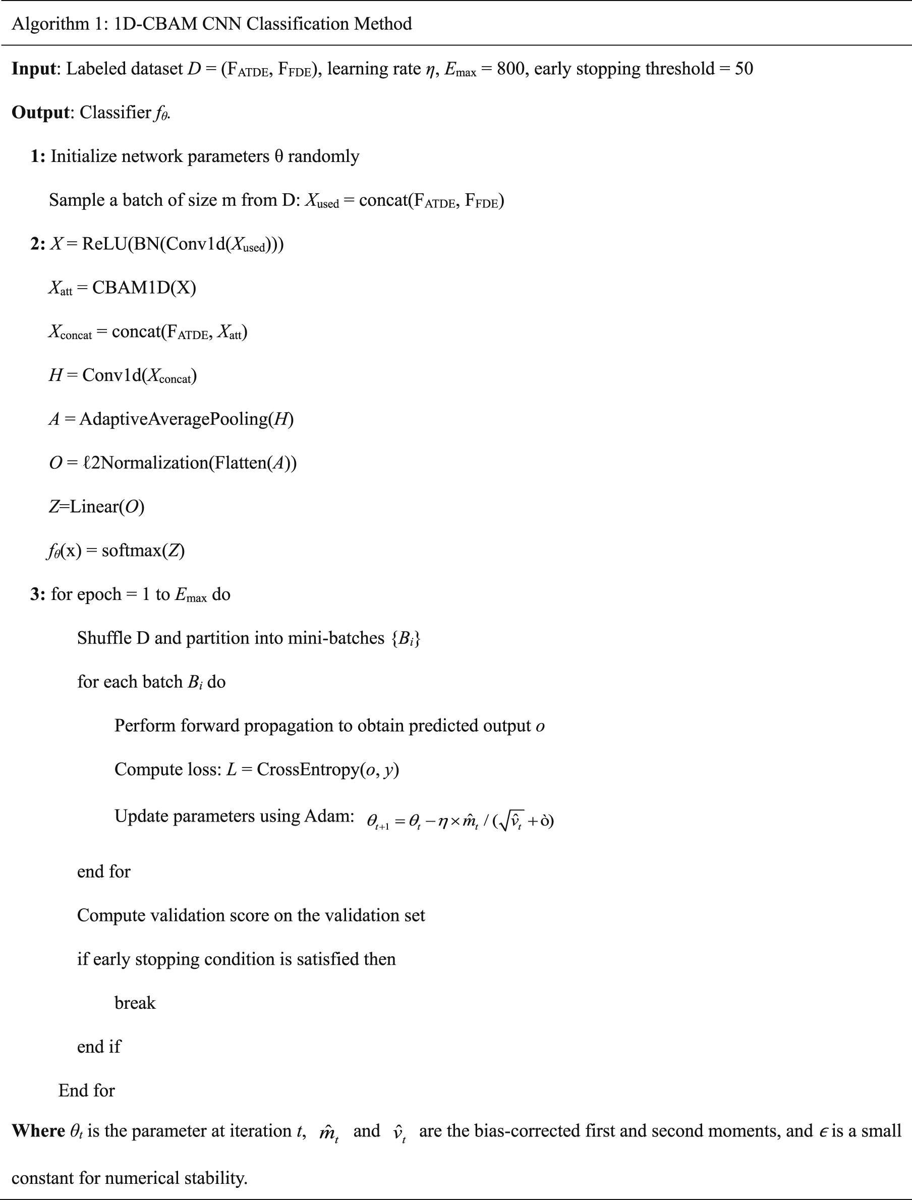
Because wheel–rail acoustic signals are highly nonstationary, simple concatenation may dilute discriminative information. CBAM is embedded into the 1D-CNN to reweight features along channel and temporal dimensions. Figure 1(c) shows the model architecture. ATDE and FDE matrices of size 18 × 10 are concatenated along the channel dimension to preserve IMF-wise correspondence and jointly represent time-domain complexity and frequency-domain energy distribution. The fused features pass through one-dimensional convolution, batch normalization, ReLU activation, and CBAM-based reweighting. Channel attention uses global average and max pooling with a multilayer perceptron to generate channel weights, while spatial attention aggregates channel-wise average and maximum responses through one-dimensional convolution to highlight informative positions. The reweighted features then pass through convolutional layers, adaptive average pooling, flattening, normalization, a fully connected layer, and Softmax for classification. Algorithm 1 gives the pseudocode.

3. Wheel–rail wear-stage diagnosis

3.1. Experiments

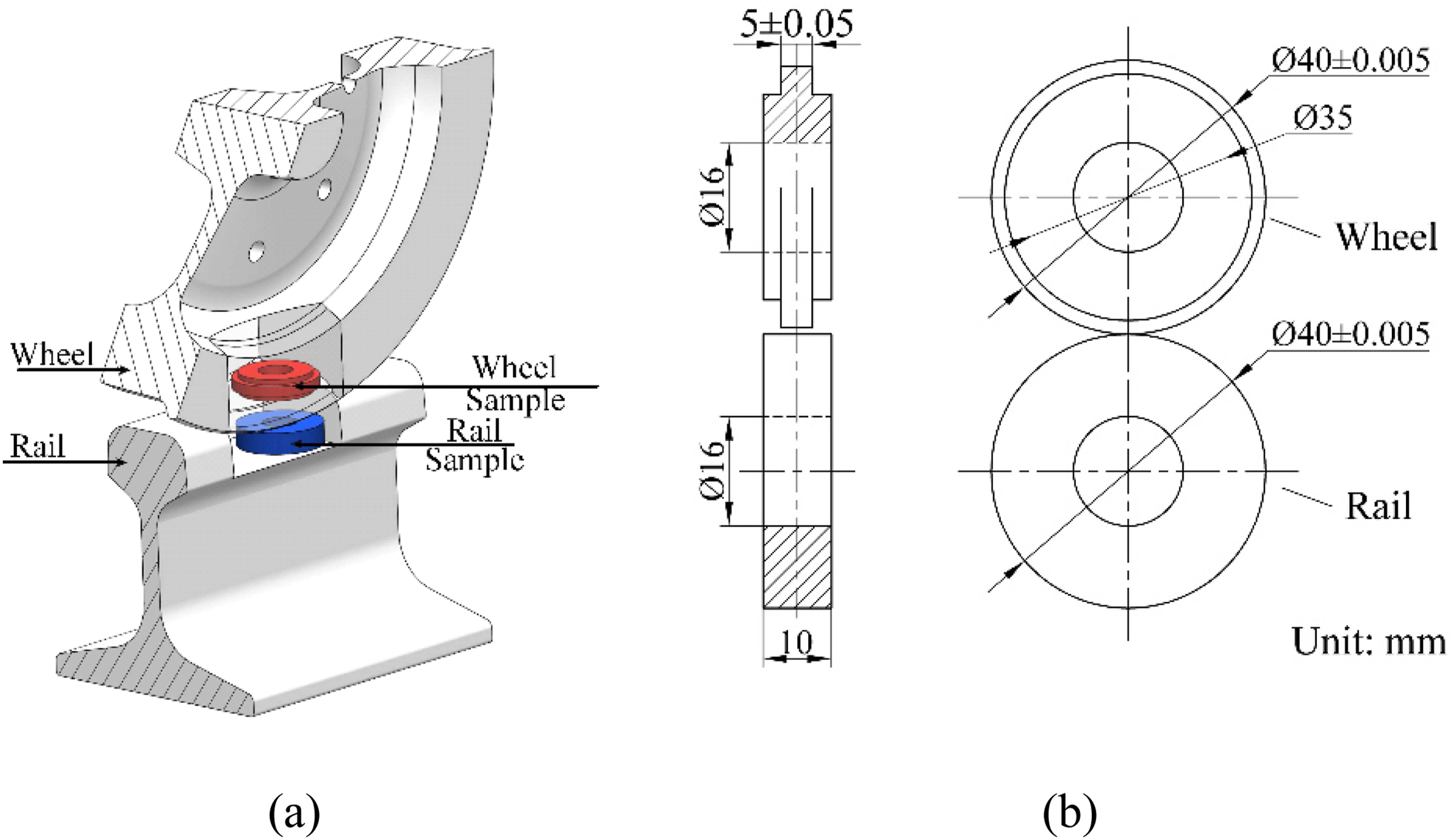
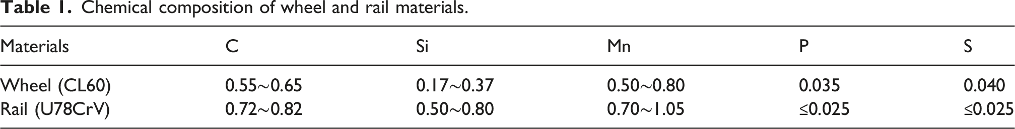
Test data were collected on a wheel–rail tribology rig (Figure 2). The wheel and rail speeds were 515 and 500 r/min, giving 3% longitudinal creepage. Based on Hertzian contact theory, a 20-t axle load corresponds to a maximum contact pressure of 641.6 MPa; the rig load was therefore set to an equivalent 580 N. The specimens were made from a U78CrV rail head and a CL60 wheel rim (Figure 3(a)). They were 40 mm in outer diameter, 16 mm in inner diameter, and 10 mm in width, with a 5 mm contact band (Figure 3(b)). Chemical compositions are listed in Table 1. The rig was pre-run for 5000 cycles. Acoustic signals were acquired using a PXDAQ24260B unit with a PXR15 sensor at 40 dB gain and 1.25 MHz.

Figure 2.

Wheel–rail friction testing platform.

Figure 3.

Schematic diagram of specimen preparation: (a) sampling schematic and (b) wheel–rail specimen specifications.

Table 1.

Chemical composition of wheel and rail materials.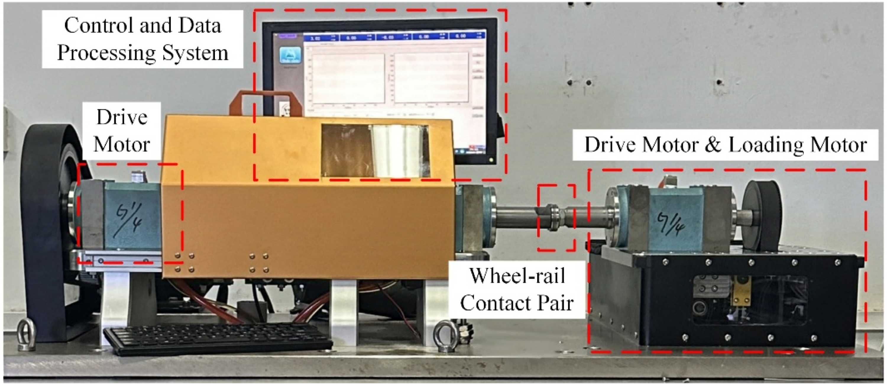

Materials	C	Si	Mn	P	S
Wheel (CL60)	0.55∼0.65	0.17∼0.37	0.50∼0.80	0.035	0.040
Rail (U78CrV)	0.72∼0.82	0.50∼0.80	0.70∼1.05	≤0.025	≤0.025

Based on surface damage and cross-sectional morphology, the life cycle was divided into four stages: Stage #1 (crack initiation), Stage #2 (crack propagation and plastic evolution), Stage #3 (accelerated damage), and Stage #4 (steady wear). Cycle ranges and sample numbers are listed in Table 2. Acoustic signals were collected by intermittent batch acquisition, with stage-wise stratified sampling to improve representativeness and reduce bias. Finally, 2000 samples were retained per stage. Each 0.12 s raw sample contained 150,000 points at 1.25 MHz. To reduce dimensionality and computation, signals were downsampled to 153.6 kHz using MATLAB resample, yielding 18,432 points per sample. Because entropy calculation depends on segment-level amplitude distributions, segment length affects probability estimation and VMD optimization stability. Preliminary tests with 512, 1024, and 2048 points showed that 1024 points gave more stable K and α with moderate cost. Each sample was therefore reshaped into an 18 × 1024 matrix. VMD was applied to each row-wise sub-signal to obtain 10 fixed modes, and ATDE/FDE generated two 18 × 10 feature matrices.

Table 2.

Stage definition and sample distribution.

Stage labels	Range of cycles	Number of samples
Stage#1	1∼5 × 10⁴	2000
Stage#2	5 × 10⁴∼10 × 10⁴	2000
Stage#3	10 × 10⁴∼16 × 10⁴	2000
Stage#4	16 × 10⁴∼21 × 10⁴	2000

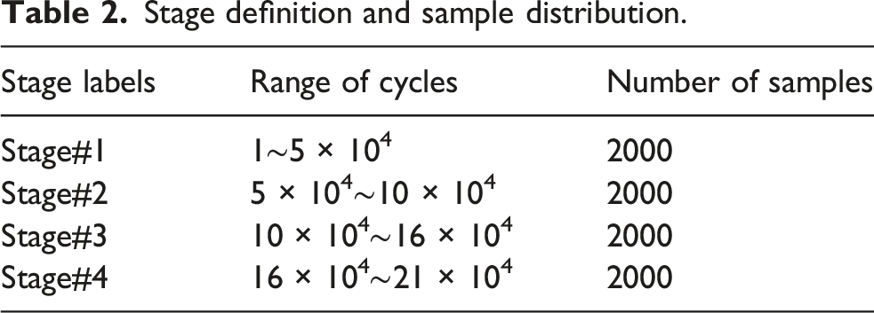
Online feasibility was assessed using a 3 s diagnostic update interval. GWO parameter search was performed offline; online diagnosis used fixed K and α for VMD and ATDE/FDE extraction. The average runtimes for VMD and entropy calculation were 0.27741 s and 0.2493 s per sample, respectively, giving 0.52671 s in total. This is below the update interval, indicating feasible online feature processing.

3.2. Wheel–rail contact acoustic signals and microscopic damage feature analysis

Figure 4 compares signals from different wear stages using energy, RMS, and CWT time–frequency maps. In Stage #1, low energy and RMS values and a concentrated CWT frequency distribution correspond to slight wear. In Stage #2, increased energy and RMS values and a broadened CWT frequency range indicate aggravated wear. In Stage #3, energy and RMS reach their maxima, and the CWT energy spreads over multiple frequency bands, suggesting severe wear. In Stage #4, energy, RMS, and CWT intensity decrease, indicating a transition toward stable wear. These results show that the selected indicators capture the stage-dependent evolution of signal characteristics. Microscopic damage evolution changes the local impact and friction states at the wheel–rail contact interface, affecting acoustic signal complexity and the corresponding multi-domain entropy features. For the selected representative samples, the mean ATDE values are higher in Stage #1 and Stage #3, at 0.7078 and 0.6688, respectively, but lower in Stage #2 and Stage #4, at 0.5803 and 0.5795. The larger ATDE standard deviations in Stage #2 and Stage #4, 0.2160 and 0.2237, indicate greater differences in time-domain complexity across temporal segments and IMF modes. The mean FDE values vary slightly from 4.9024 to 4.9568, complementing the characterization of inter-modal differences in frequency-domain energy distribution. Thus, multi-domain entropy features indirectly reflect the stage-wise evolution of wear damage through acoustic signal complexity and frequency-domain energy distribution.

Figure 4.

Analysis of wheel–rail contact acoustic signals.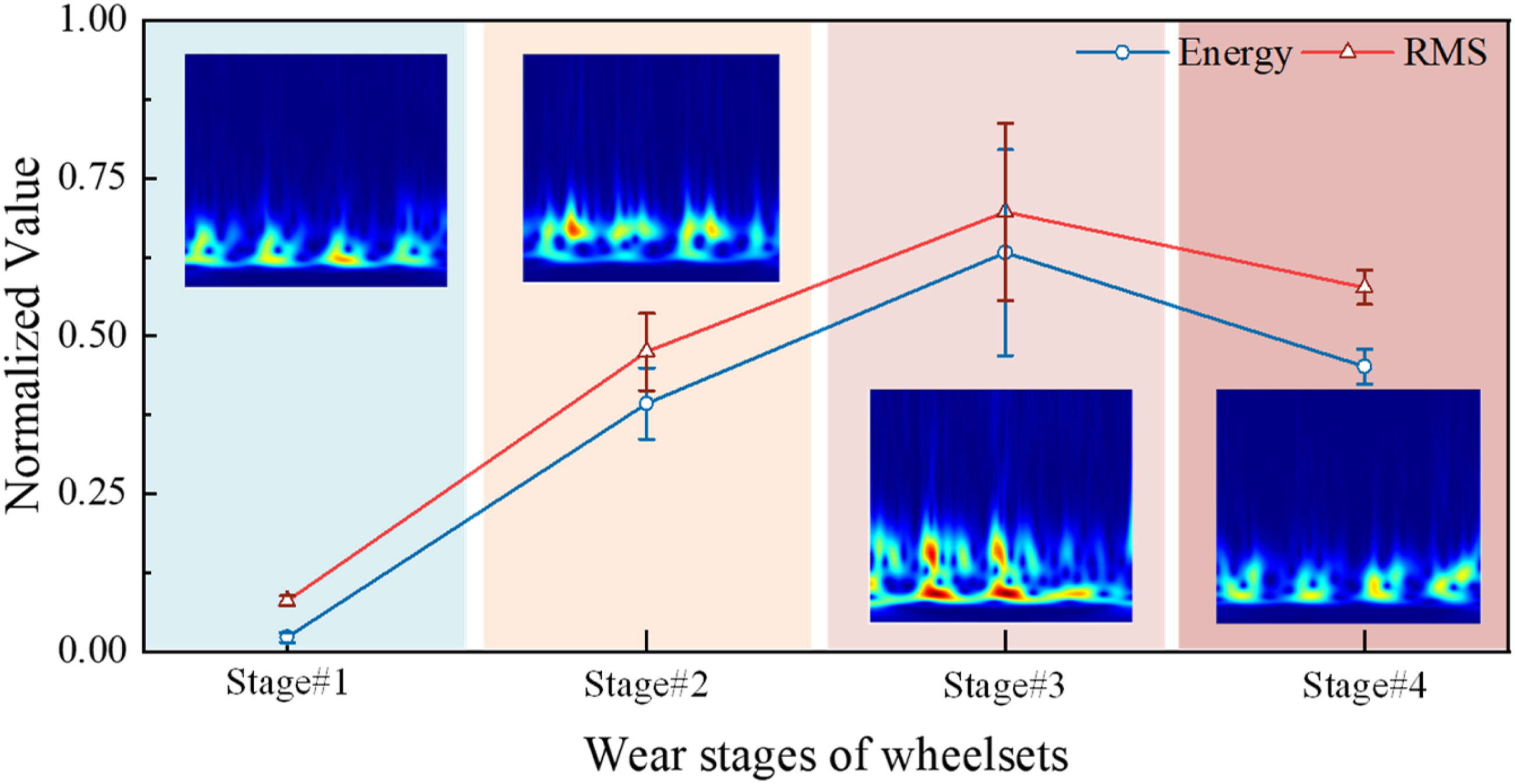

Figure 5 shows optical micrographs of wheel cross-sectional damage and the corresponding plastic deformation morphologies at different cycle intervals. N1–N4 correspond to 5 × 10⁴, 10 × 10⁴, 16 × 10⁴, and 21 × 10⁴ cycles, respectively. At N1 node, fatigue cracks appear and propagate obliquely into the substrate. At N2 node, the crack angle and depth increase, and tangential loading induces a plastically deformed surface layer. Cracks then extend inward along the plastic flow lines. At N3 node, crack density increases, surface spalling becomes evident, and the plastic layer thickens by about 6.2 µm with increased roughness. At N4 node, a complex crack network and local spalling are observed. In some regions, changes in plastic flow direction alter the crack propagation angle, while the plastic layer thickness becomes relatively stable (Cvetkovski et al., 2014).

Figure 5.

Wheel cross-sectional damage evolution showing paired optical microscopy (OM) images and plastic deformation layers at different cycle nodes: (a) N1, (b) N2, (c) N3, and (d) N4.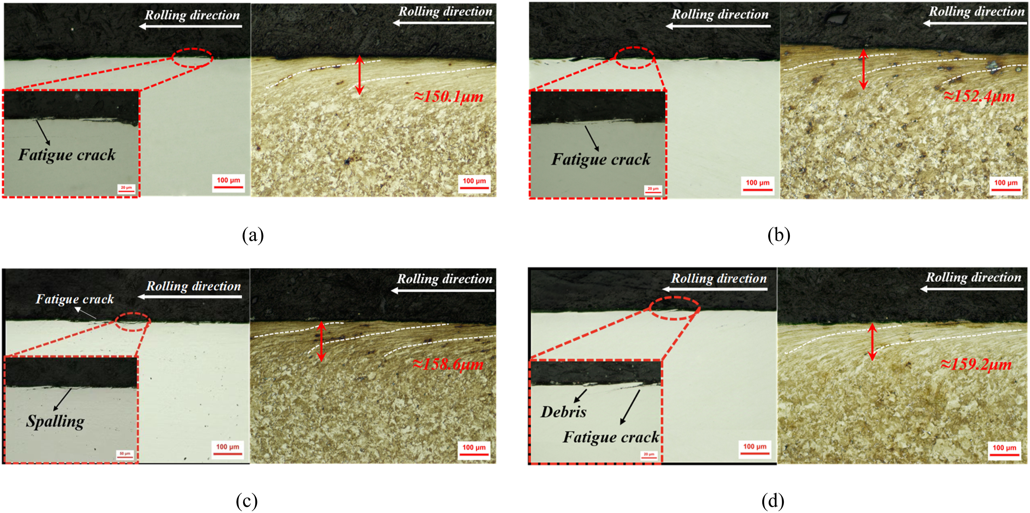

Figure 6 shows optical micrographs of rail cross-sectional damage and the corresponding plastic deformation morphologies at different cycle numbers. At N1 node, cracks begin to propagate along the rolling direction. At N2 node, plastic flow lines extend inward, but the cracks remain limited and the plastic layer changes only slightly. At N3 node, crack density increases, multilayer cracks appear, and fatigue cracks further extend into the subsurface layer, with a 3.1 µm change in the plastic deformation layer. At N4 node, crack number decreases, the flow lines become nearly parallel to the surface, and crack propagation also tends to be parallel, indicating a more stable wear state. A lower stress level may suppress further crack growth.

Figure 6.

Rail cross-sectional damage evolution showing paired optical microscopy (OM) images and plastic deformation layers at different cycle nodes: (a) N1, (b) N2, (c) N3, and (d) N4.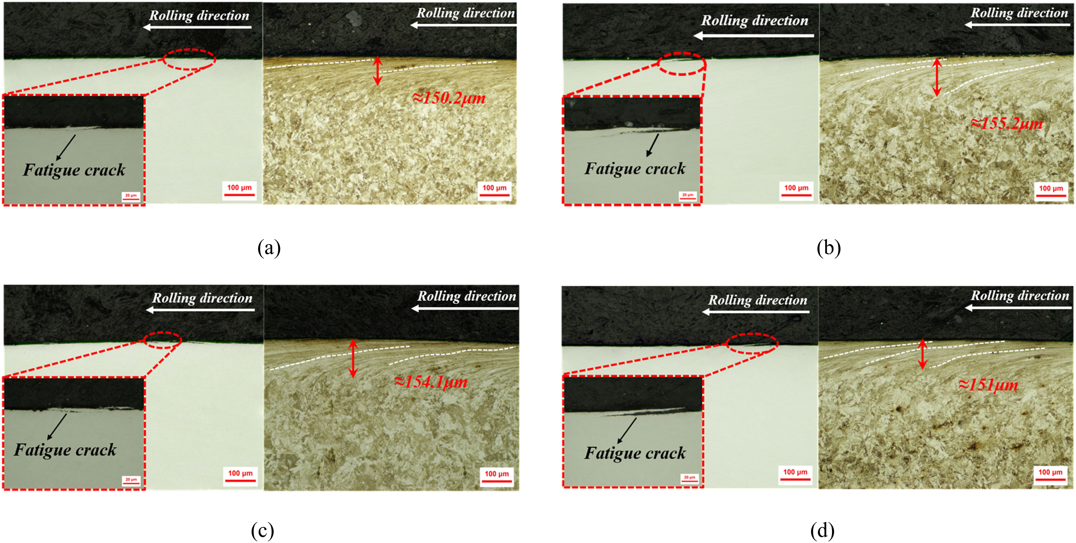

Figure 7 presents the three-dimensional surface morphologies of the wheel and rail at different cycle stages. For the wheel, large spalling pits are observed at N1 node. At N3 node, the pit size exceeds 100 µm and the depth exceeds 15 µm. At N4 node, the pit area and depth decrease, and the surface becomes smoother. For the rail, a spalling pit appears at N2 node, with a width of about 100 µm and a depth of about 4 µm. At N3 node, the pit area decreases while the depth remains nearly unchanged. At N4, the surface becomes smoother and spalling pits occur much less frequently. Figure 8 shows the evolution of areal roughness Sa, which is consistent with the wear process (Benoit et al., 2016). For the wheel, Sa is lowest at N1 node, at 1.954 µm, reaches 2.802 µm at N3 node, and then decreases to 2.34 µm in the steady wear stage. For the rail, Sa increases from 0.53 µm at N1 node to 0.998 µm at N3 node, and then decreases to 0.698 µm. This trend suggests that wear becomes dominant, whereas the contribution of crack propagation weakens.

Figure 7.

Three-dimensional surface topographies of worn wheel (left) and rail (right) surfaces at different cycle nodes: (a) N1, (b) N2, (c) N3, and (d) N4.

Figure 8.

Surface roughness of the wheel and rail specimens plotted with different wear cycles.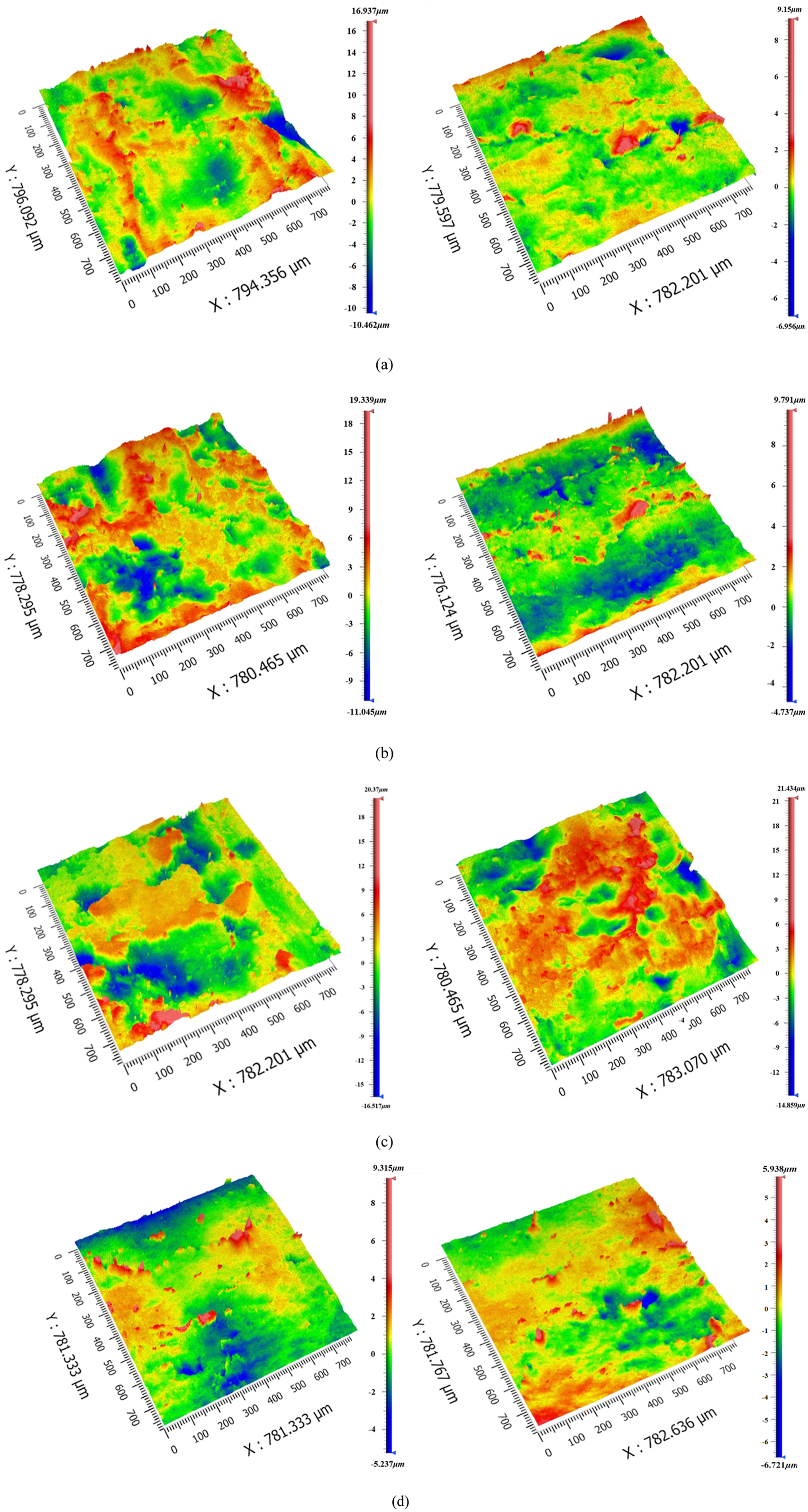

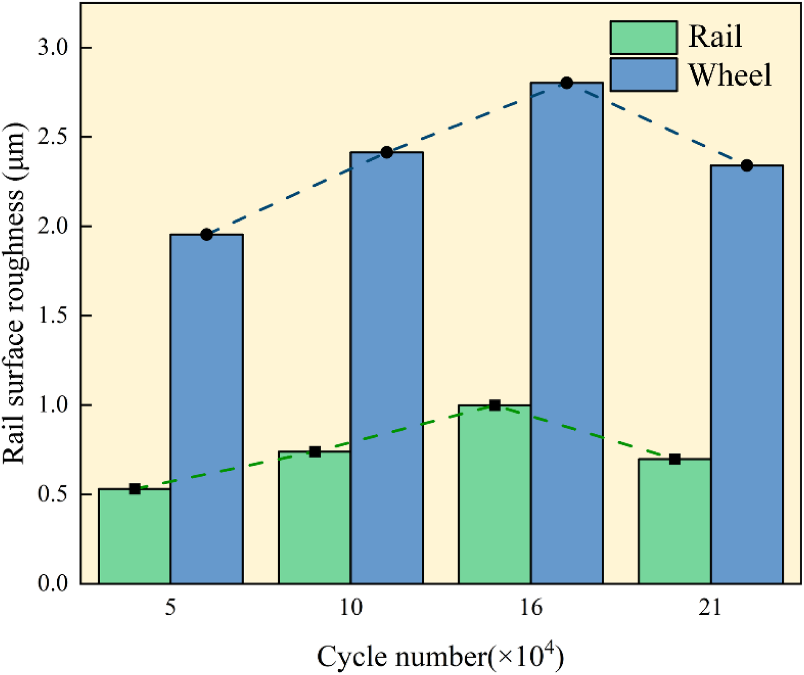
Figure 9 summarizes the SEM observations of stage-wise damage evolution in the wheel and rail. For the wheel, adhesive wear dominates at N1 node, with block-like wear debris. At N2 node, adhesion weakens and microcracks appear on a relatively smooth surface. At N3 node, cracks become more evident, and large, deep spalling pits form, consistent with fatigue damage accumulation. At N4 node, crack number decreases and the surface becomes flatter. Severe wear may suppress further crack initiation, making wear the dominant mechanism. For the rail, cracks are limited at N1 node, with only slight local spalling. At N2 node, crack density increases, and larger but shallow spalling pits appear. At N3 node, rapid crack propagation is accompanied by aggravated damage. At N4 node, crack number decreases, spalling disappears, and the surface becomes relatively flat. Severe wear may suppress further crack propagation (Hu et al., 2021).

Figure 9.

SEM images of worn wheel (left) and rail (right) surfaces at different cycle nodes: (a) N1, (b) N2, (c) N3, and (d) N4.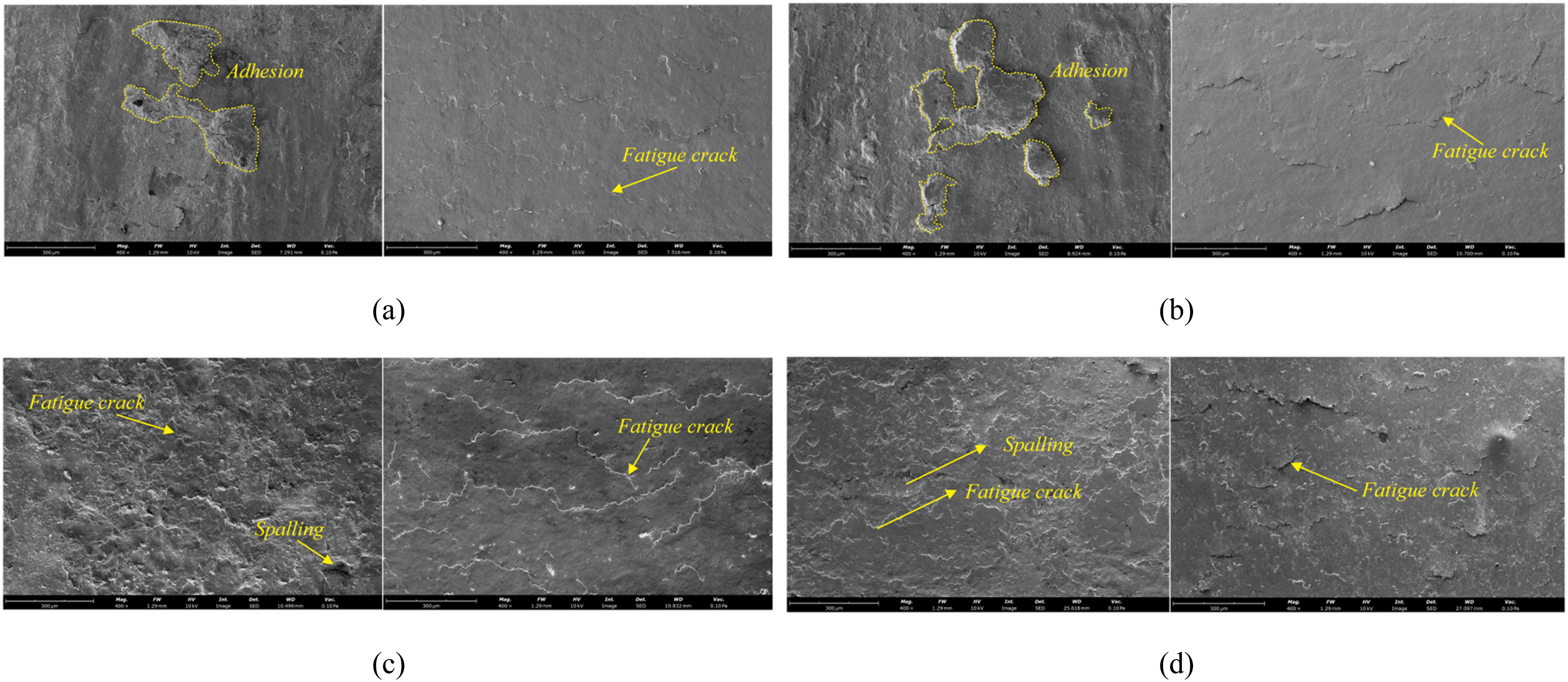

3.3. Fault diagnosis and performance assessment

Experiments were implemented in PyTorch 1.13 with Python 3.9 on an Intel(R) Core(TM) i7-14700KF CPU (3.40 GHz). Training was capped at 800 epochs with early stopping after 50 epochs without validation improvement; the best checkpoint was used for testing. Grid search was conducted for learning rate {10–3, 10–4, 10–5} and batch size {64, 128, 256}, and the best configuration was used.

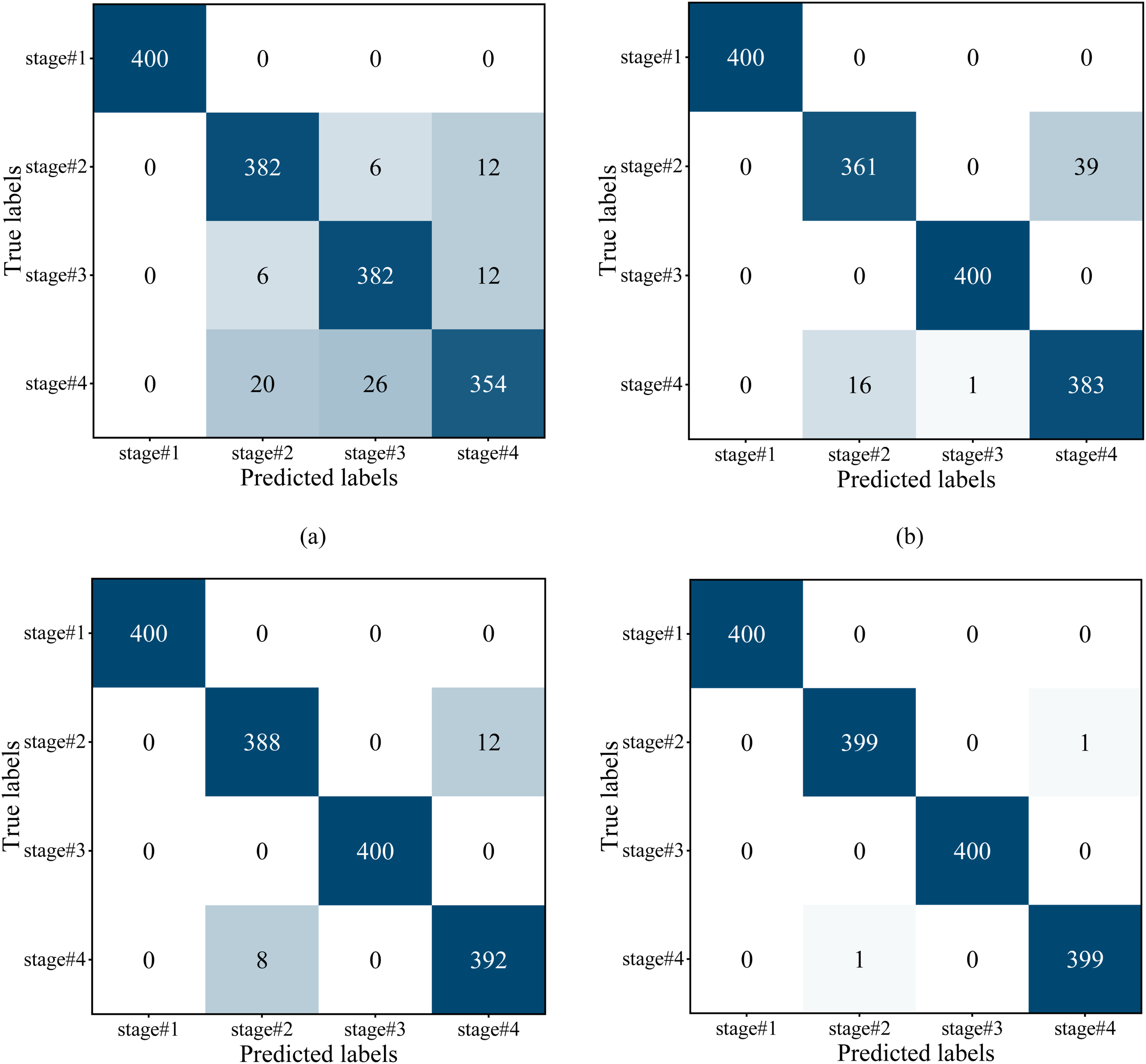
Ablation experiments evaluated the contributions of ATDE, FDE, and CBAM by removing each module individually. Figure 10 reports accuracies under 6:2:2, 8:1:1, and 7:2:1 splits, with models denoted as w/o ATDE, w/o FDE, w/o CBAM, and Full model. Figure 11 presents the confusion matrix for the 6:2:2 split. The Full model achieves 99.88% test accuracy and distinguishes the four stages effectively. Stage #1 and Stage #3 are classified with 100% accuracy, while only one sample is confused between Stage #2 and Stage #4, consistent with their similar damage morphology and signal features. Overall, ATDE, FDE, and CBAM all improve performance, with ATDE contributing most and CBAM further enhancing discriminative feature responses.

Figure 10.

Results of the ablation experiment.

Figure 11.

Confusion matrix for the ablation experiment on the Wheel–Rail Friction Dataset: (a) w/o ATDE, (b) w/o FDE, (c) w/o CBAM, and (d) Full model.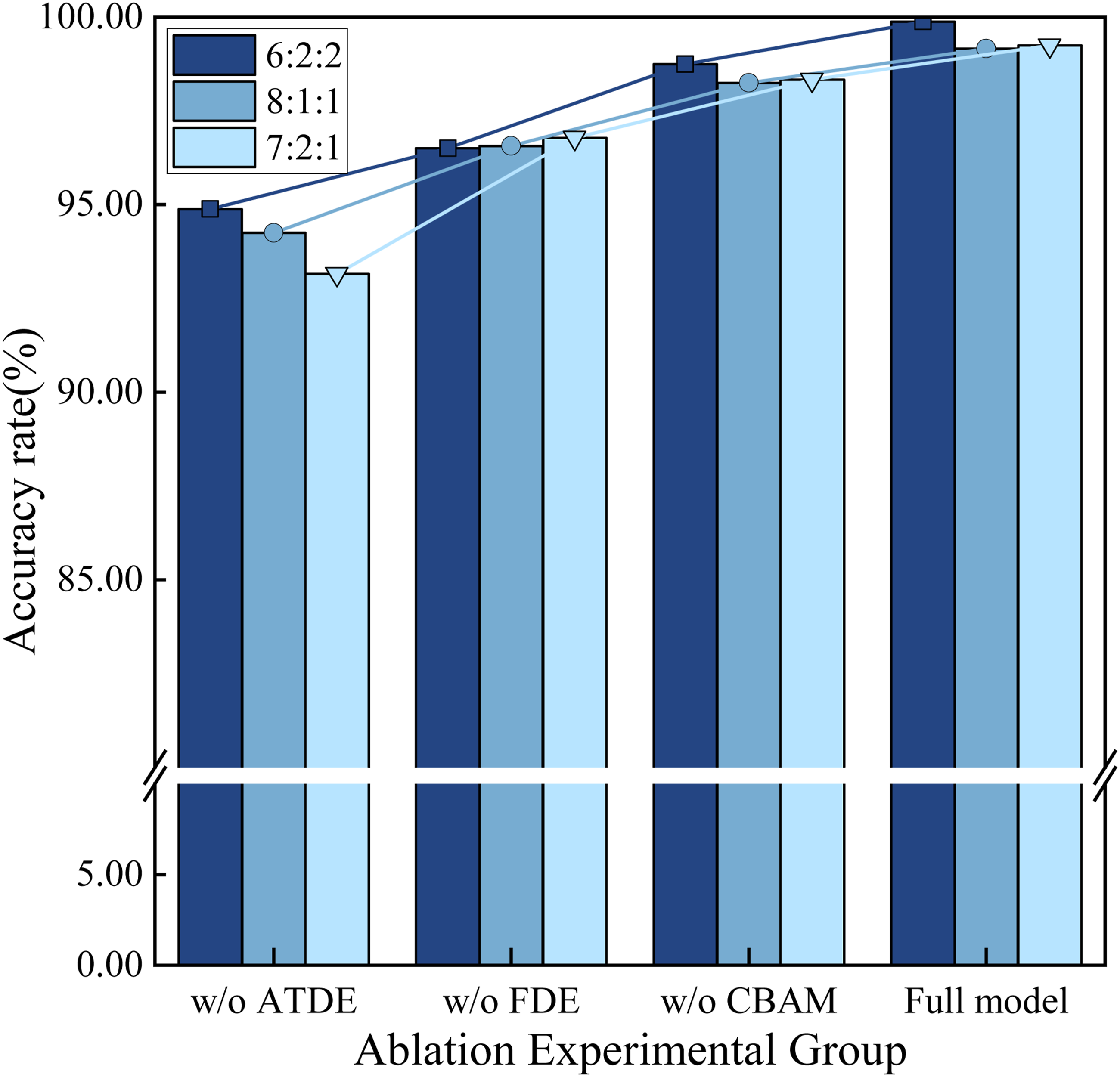

t-SNE was used to visualize feature evolution across network layers. In Figure 12, each point denotes a test sample, and colors indicate wear stages. From the input layer to the pre-classification space, intra-class samples become more compact, inter-class overlap decreases, and class boundaries become clearer, indicating progressively enhanced feature representation.

Figure 12.

t-SNE visualization of feature-space distributions at different model stages.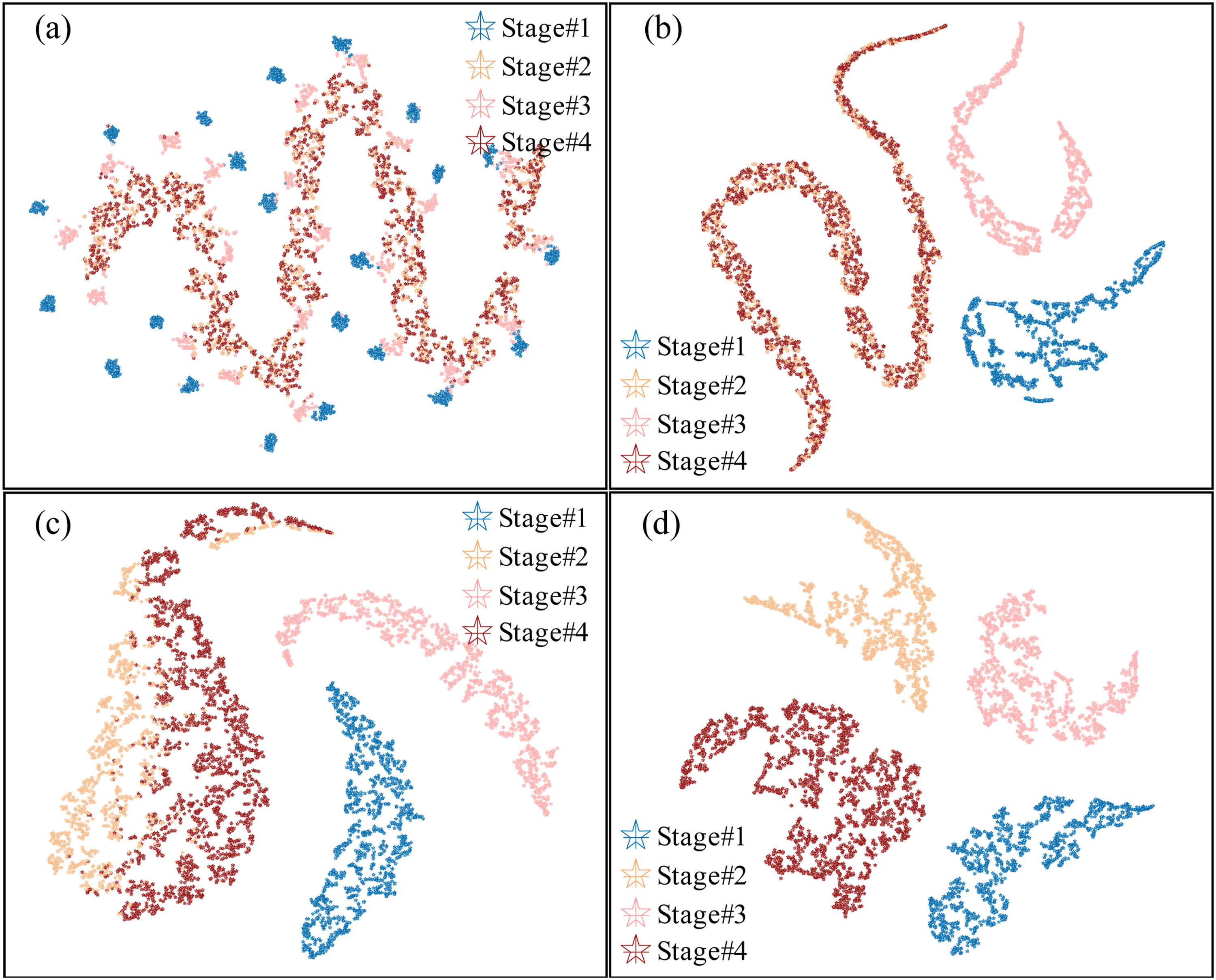

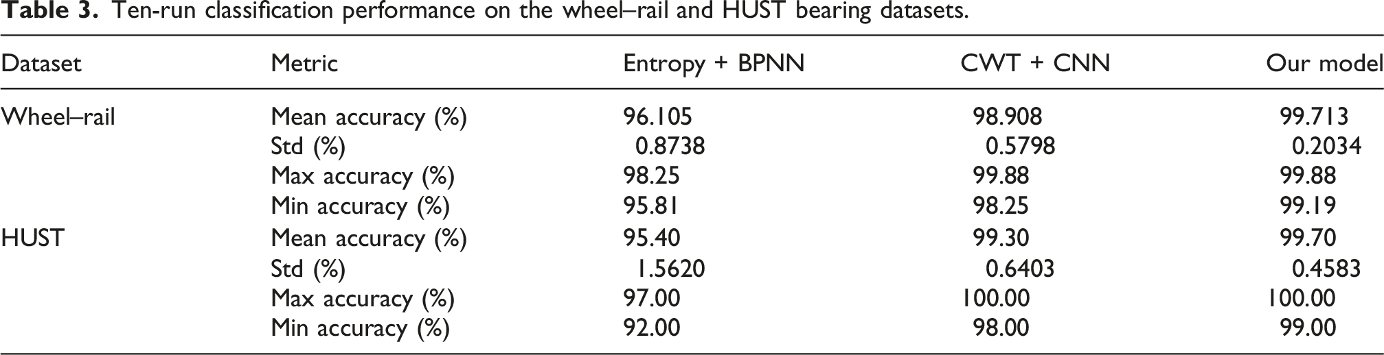
To evaluate stability, Entropy + BPNN, CWT + CNN, and the proposed model were trained and tested 10 times using the same split and strategy. All models were first tuned on the validation set; the selected hyperparameters were then fixed for repeated runs and SNR tests. As shown in Table 3, the proposed model achieves the highest mean accuracy of 99.713%, the lowest standard deviation of 0.2034%, and a minimum accuracy of 99.19%. Entropy + BPNN and CWT + CNN obtain lower mean accuracies of 96.105% and 98.908%, respectively, with larger fluctuations. These results indicate that the proposed model improves both recognition accuracy and training stability under different random initializations.

Table 3.

Ten-run classification performance on the wheel–rail and HUST bearing datasets.

Dataset	Metric	Entropy + BPNN	CWT + CNN	Our model
Wheel–rail	Mean accuracy (%)	96.105	98.908	99.713
	Std (%)	0.8738	0.5798	0.2034
	Max accuracy (%)	98.25	99.88	99.88
	Min accuracy (%)	95.81	98.25	99.19
HUST	Mean accuracy (%)	95.40	99.30	99.70
	Std (%)	1.5620	0.6403	0.4583
	Max accuracy (%)	97.00	100.00	100.00
	Min accuracy (%)	92.00	98.00	99.00

White noise was added at SNRs of 0, 5, and 10 dB to evaluate robustness. As shown in Figure 13, all models improve as SNR increases. The proposed model reaches 93.686%, 95.975%, and 97.863% mean accuracy at 0, 5, and 10 dB, outperforming both baselines and maintaining over 93% accuracy even at 0 dB. This indicates stronger discriminative stability under noise.

Figure 13.

Noise robustness comparison under different SNR levels on the Wheel–Rail Friction dataset.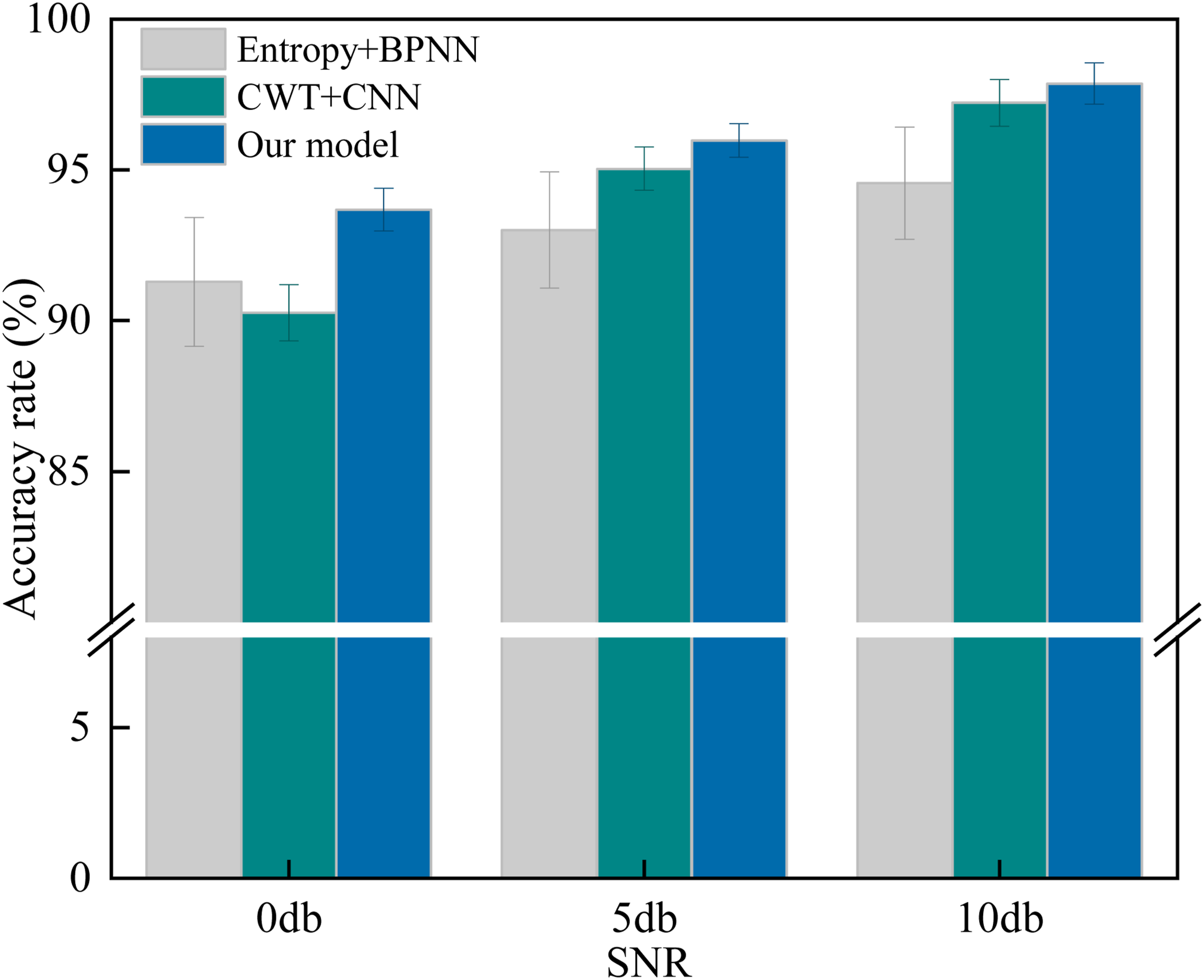

Table 4 compares model complexity and performance on the wheel–rail dataset. Inference time refers only to classifier forward propagation. Entropy + BPNN has the lowest computational cost but lower accuracy. CWT + CNN also reaches 99.88% accuracy but requires far more parameters, memory, and inference time. The proposed model uses only 13,848 parameters, has a size of 58.82 KB, and requires 0.014 s for forward inference while achieving 99.88% accuracy. FLOPs measure theoretical floating-point operations, whereas actual inference time is affected by model architecture, tensor scheduling, and operator implementation. Thus, the proposed model substantially reduces overhead compared with image-input models while preserving accuracy.

Table 4.

Model complexity and performance comparison on two datasets.

Dataset	Metric	Entropy + BPNN	CWT + CNN	Our model
Wheel–rail	Params	23,364	5,109,188	13,848
	Model size (KB)	93.29	18,490	58.82
	FLOPs (k)	23.296	1,307,000	133.87
	Inference time (s)	0.0012	5.4700	0.014
	Best accuracy	98.25%	99.88%	99.88%
HUST	Params	11,909	5,109,317	2550
	Model size (KB)	143.98	19,958.27	15.51
	FLOPs (k)	11.9040	653,679	35.346
	Inference time (s)	0.0001	0.6220	0.0004
	Best accuracy	97%	100%	100%

From an engineering application perspective, the proposed method can support periodic online monitoring in a cloud–edge collaborative mode. VMD decomposition, ATDE/FDE feature extraction, and lightweight CNN analysis are performed on the cloud side, while the edge side receives diagnostic results for alarm triggering or data logging. The results show that the proposed method balances recognition accuracy, model overhead, and deployment cost, making it suitable for wheel–rail wear-state recognition under resource constraints.

4. Validation on the HUST bearing dataset

To assess the applicability of the proposed method beyond the wheel–rail wear dataset, cross-dataset validation was conducted using the public HUST bearing dataset from Huazhong University of Science and Technology. This test evaluates model consistency across different mechanical components and data sources.

4.1. Experimental data description

Five bearing conditions under the 20 Hz operating condition were selected: Normal, M-Ball, M-Comb, M-Inner, and M-Outer. The sampling frequency was 25.6 kHz (Zhao et al., 2024). For fair comparison, vibration signals from the same measurement direction were used. Each condition contained 100 samples, with 2048 points per sample. Feature construction and model training followed the same procedure as that used for the wheel–rail wear dataset.

4.2. Model training and fault diagnosis

Figure 14 shows the HUST ablation results. The Full model performs best under all data splits, reaching 100% for 6:2:2 and 8:1:1 and 98% for 7:2:1. Removing ATDE causes the largest decrease, confirming the dominant role of time-domain complexity. Removing FDE also degrades accuracy, while removing CBAM causes a slight decrease, indicating the benefit of attention-based reweighting. Table 3 gives the 10-run results of the three models on the HUST dataset. The proposed model obtains the highest mean accuracy of 99.70%, the lowest standard deviation of 0.4583%, and a minimum accuracy of 99.00%, compared with 99.30% for CWT + CNN and 95.40% for Entropy + BPNN. These results demonstrate high accuracy and stable repeated-run performance under noise-free conditions.

Figure 14.

Ablation experiment results on the HUST bearing dataset.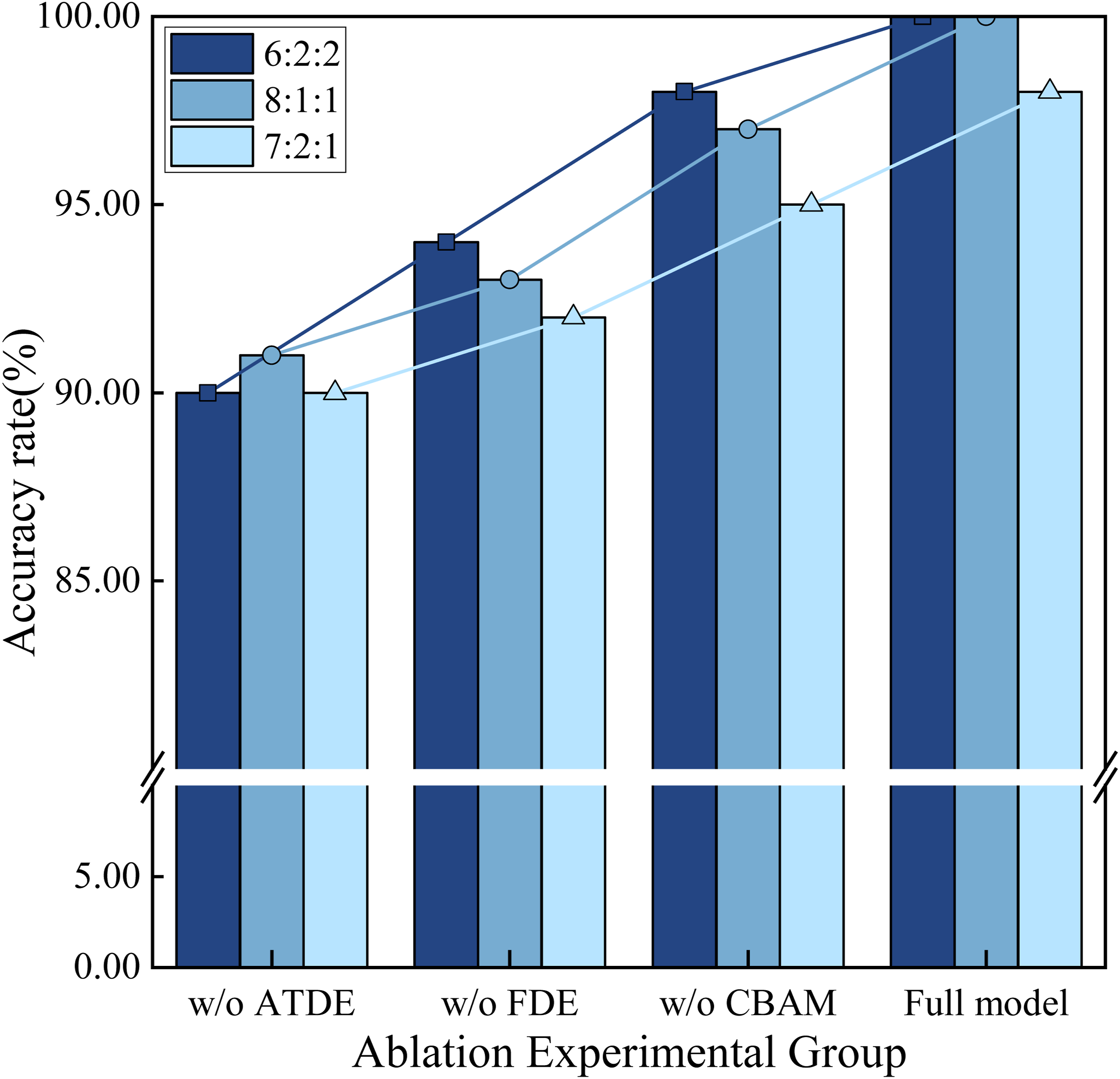

Figure 15 shows the noise robustness results under different SNRs. As the SNR increases from 0 dB to 10 dB, all models show an overall improvement in accuracy. The proposed model achieves the highest or comparable accuracy across noise levels with smaller fluctuations, suggesting that the multi-domain entropy features and attention mechanism maintain strong discriminative ability under noise disturbance.

Figure 15.

Noise robustness comparison under different SNR levels on the HUST bearing dataset.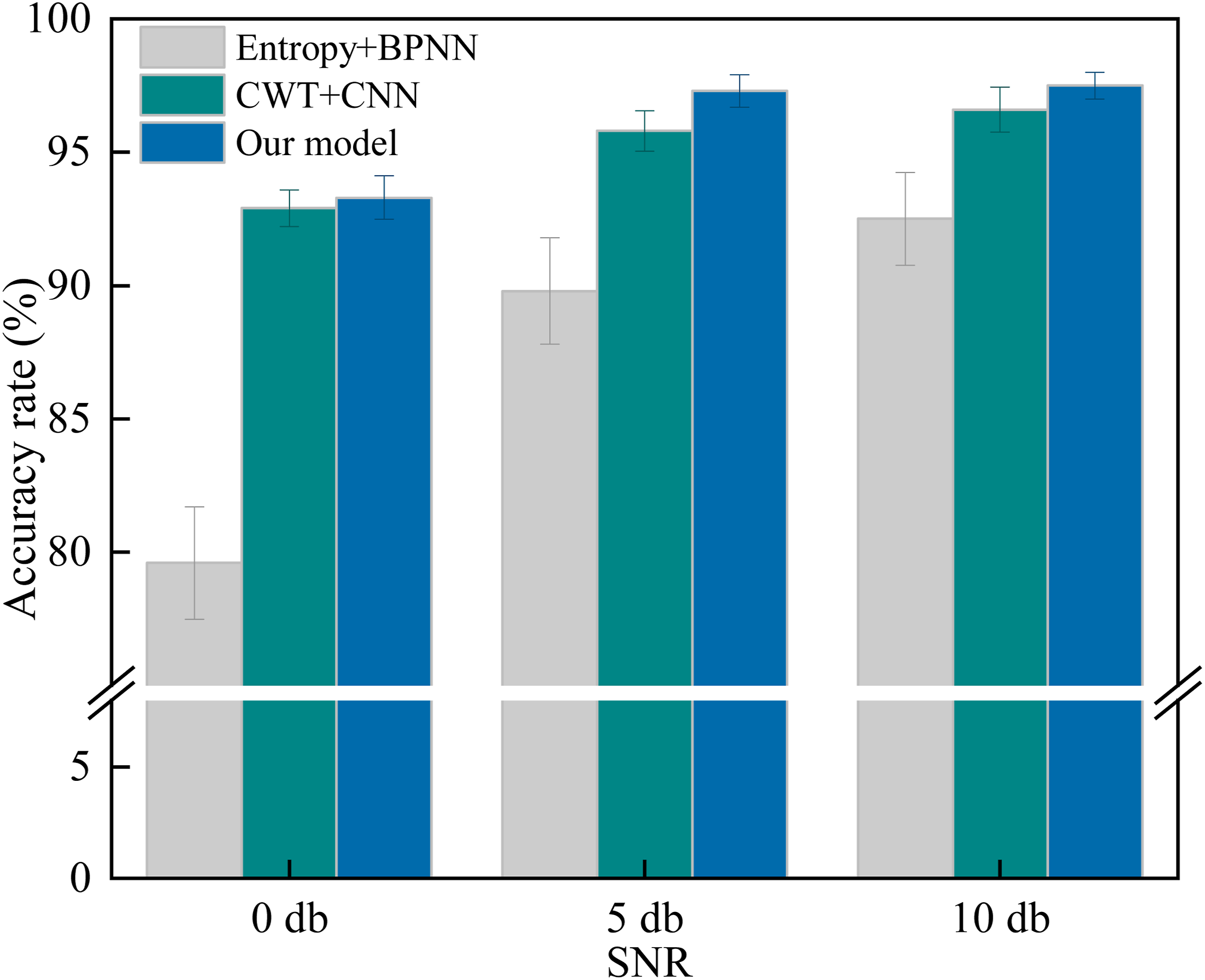

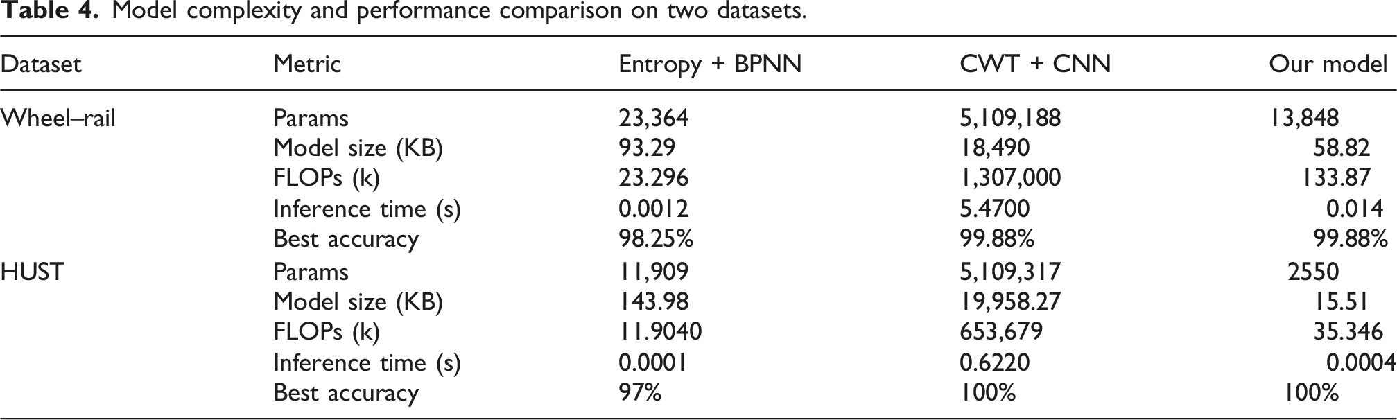
Table 4 further compares model complexity and performance. The proposed model uses only 2550 parameters and has a size of 15.51 KB, both lower than those of the two baselines. Its FLOPs are 35.346 k, higher than Entropy + BPNN but much lower than CWT + CNN. Its inference time is 0.0004 s, slightly higher than Entropy + BPNN but far lower than CWT + CNN at 0.6220 s. Overall, the proposed model provides high diagnostic stability and low model overhead on the HUST dataset.

5. Conclusion

This study develops a diagnostic framework for heavy-haul railway wheel–rail contact friction-state recognition by integrating GWO-VMD, multi-domain entropy features, and an attention-enhanced lightweight network. The main conclusions are as follows.

(1) A signal representation procedure combining offline parameter optimization and online feature extraction is established. GWO determines the VMD parameters offline, while fixed parameters are used online for wheel–rail acoustic signal decomposition and ATDE/FDE feature extraction. ATDE describes time-domain complexity, and FDE describes frequency-domain energy distribution. The CBAM-enhanced lightweight 1D-CNN enables adaptive feature weighting and fast classification.

(2) On the wheel–rail dataset, the proposed method achieves a favorable balance among accuracy, stability, and model overhead. It reaches 99.88% test accuracy in the four-stage wear classification task and maintains high performance under different SNRs, indicating good stability and noise robustness. Compared with time–frequency image-based models, the classifier reduces forward inference time by about 99.74% while maintaining 99.88% accuracy, with only 13,848 parameters. These results support low-latency wheel–rail wear classification under resource constraints.

(3) Validation on the public HUST bearing dataset further suggests applicability to different mechanical diagnostic tasks. In the five-class task, the method achieves 99.70% mean accuracy over ten runs, a maximum accuracy of 100%, a model size of 15.51 KB, and a classifier forward inference time of 0.0004 s. Overall, the method offers a low-overhead solution for periodic wheel–rail wear-state monitoring, although further validation under more complex load, speed, and environmental conditions is required.

Footnotes

ORCID iDs

Hao Wu

Yuxing Li

Funding

The authors disclosed receipt of the following financial support for the research, authorship, and/or publication of this article: This work was supported by the National Natural Science Foundation of China (Grant No 52567002 and 62571424) and the Ganpo Juncai Support Program, Jiangxi (Grant No 20243BCE51071).

Declaration of conflicting interests

The authors declared no potential conflicts of interest with respect to the research, authorship, and/or publication of this article.

Data Availability Statement

Mingxue Shen will handle all correspondence at all stages of refereeing, publication, and post-publication. The corresponding author is responsible for any future queries related to the methodology, data, and results of this study. The provided email address is valid and will be kept up to date throughout the process.*

References

Bai

Liu

Lin

, et al. (2024) SNR enhancement method for Φ-OTDR system based on Sdr_SampEn-BiPSO-SVD algorithm. IEEE Transactions on Instrumentation and Measurement 73: 1–12. https://doi.org/10.1109/TIM.2023.3338685

Benoit

Salima

Marion

(2016) Multiscale characterization of head check initiation on rails under rolling contact fatigue: mechanical and microstructure analysis. Wear 366: 383–391. https://doi.org/10.1016/j.wear.2016.06.019

Chen

Feng

Chen

, et al. (2025) A machine learning-based interpretable fault diagnosis method for rolling bearings under unbalanced samples. Engineering Applications of Artificial Intelligence 158: 111505. https://doi.org/10.1016/j.engappai.2025.111505

Cvetkovski

Ahlstrom

Norell

, et al. (2014) Analysis of wear debris in rolling contact fatigue cracks of pearlitic railway wheels. Wear 314(1–2): 51–56. https://doi.org/10.1016/j.wear.2013.11.049

Dou

Lin

Guo

(2023) A novel feature for fault classification of rotating machinery: ternary approximate entropy for original, shuffle and surrogate data. Machines 11(2): 172. https://doi.org/10.3390/machines11020172

Firlik

Staskiewicz

Slowinski

(2023) Thermal imaging of the wheel-rail interface. Proceedings of the Institution of Mechanical Engineers, Part F: Journal of Rail and Rapid Transit 237(9): 1195–1204. https://doi.org/10.1177/09544097231155573

Gong

Wang

, et al. (2023) Lightweight fault diagnosis method in embedded system based on knowledge distillation. Journal of Mechanical Science and Technology 37(11): 5649–5660. https://doi.org/10.1007/s12206-023-1007-3

Shi

(2023) IDSN: a one-stage interpretable and differentiable STFT domain adaptation network for traction motor of high-speed trains cross-machine diagnosis. Mechanical Systems and Signal Processing, Epub ahead of print 20 October 2023. DOI: 10.1016/j.ymssp.2023.110846.

Zhou

Ding

, et al. (2021) Microstructure evolution of railway pearlitic wheel steels under rolling-sliding contact loading. Tribology International 154: 106685. https://doi.org/10.1016/j.triboint.2020.106685

10.

Gao

Shao

, et al. (2025) Multi-scale quadratic convolutional neural network for bearing fault diagnosis based on multi-sensor data fusion. Nonlinear Dynamics, Epub ahead of print 2 February 2025. DOI: 10.1007/s11071-025-10918-6.

11.

Jiang

Wang

, et al. (2023) An interpretable convolutional neural network with multi-wavelet kernel fusion for intelligent fault diagnosis. Journal of Manufacturing Systems, Epub ahead of print 11 July 2023. DOI: 10.1016/j.jmsy.2023.06.015.

12.

Kocur

Thaler

Markert

(2024) Acoustic source localization by deep-learning attention-based modulation of microphone array data. NDT & E International 148: 103233. https://doi.org/10.1016/j.ndteint.2024.103233

13.

Chen

, et al. (2017) Independence-oriented VMD to identify fault feature for wheel set bearing fault diagnosis of high speed locomotive. Mechanical Systems and Signal Processing 85: 512–529. https://doi.org/10.1016/j.ymssp.2016.08.042

14.

Liu

, et al. (2020) An optimized VMD method and its applications in bearing fault diagnosis. Measurement 166: 108185. https://doi.org/10.1016/j.measurement.2020.108185

15.

Zhou

Jiao

(2025) Hermite interpolation multiscale adaptive dispersion entropy and its application in feature extraction. IEEE Transactions on Instrumentation and Measurement 74: 1–13. https://doi.org/10.1109/TIM.2025.3556913

16.

Liu

Zhou

Wang

, et al. (2026) Research on a bridge crane rail fault diagnosis method integrating HO-VMD and RS-BP. Journal of Vibration and Control, Epub ahead of print 10 January 2026. DOI: 10.1177/10775463261416550.

17.

Liang

, et al. (2025) Fault diagnosis method for train bogie axlebox based on deep learning feature fusion of CWT-MVGG. Journal of Vibration and Control, Epub ahead of print 18 November 2025. DOI: 10.1177/10775463251399722.

18.

Montinaro

Epasto

Cerniglia

, et al. (2019) Laser ultrasonics inspection for defect evaluation on train wheel. NDT & E International 107: 102145. https://doi.org/10.1016/j.ndteint.2019.102145

19.

Nicholson

Davis

(2012) Modelling of the response of an ACFM sensor to rail and rail wheel RCF cracks. NDT & E International 46: 107–114. https://doi.org/10.1016/j.ndteint.2011.11.010

20.

Noman

Ali

, et al. (2024) A novel nonlinear dynamic measure for early detection of bearing fault using weighted squared envelope-based symbolic Lempel-Ziv complexity. IEEE Transactions on Instrumentation and Measurement 73: 1–16. https://doi.org/10.1109/TIM.2024.3463030

21.

Zhang

, et al. (2024) Study on the mechanism of wheel asymmetric wear of heavy-haul freight vehicles. Tribology Transactions 67(2): 294–310. https://doi.org/10.1080/10402004.2024.2312244

22.

Rostaghi

Azami

(2016) Dispersion entropy: a measure for time-series analysis. EEE Signal Processing Letters 23(5): 610–614. https://doi.org/10.1109/LSP.2016.2542881

23.

Shen

C-H

(2022) Acoustic emission based grinding wheel wear monitoring: signal processing and feature extraction. Applied Acoustics 196: 108863. https://doi.org/10.1016/j.apacoust.2022.108863

24.

Song

Wang

Chen

(2018) Vibration-based intelligent fault diagnosis for roller bearings in low-speed rotating machinery. IEEE Transactions on Instrumentation and Measurement 67(8): 1887–1899. https://doi.org/10.1109/TIM.2018.2806984

25.

Sudarshan

Ramachandra

Ojha

, et al. (2024) DCEnt-PredictiveNet: a novel explainable hybrid model for time series forecasting. Neurocomputing 608: 128389. https://doi.org/10.1016/j.neucom.2024.128389

26.

Tang

Jiang

, et al. (2025) A fault identification method of hydraulic pump fusing long short-term memory and synchronous compression wavelet transform. Applied Acoustics 232: 110553. https://doi.org/10.1016/j.apacoust.2025.110553

27.

Tehranchi

Hamidi

Eftekhari

, et al. (2011) The inspection of magnetic flux leakage from metal surface cracks by magneto-optical sensors. Sensors and Actuators A: Physical 172(2): 365–368. https://doi.org/10.1016/j.sna.2011.09.010

28.

Wang

, et al. (2025) Rolling bearing fault diagnosis based on multi-domain features and whale optimized support vector machine. Journal of Vibration and Control 31(5–6): 708–720. https://doi.org/10.1177/10775463241231344

29.

Wang

You

, et al. (2025) Chatter feature extraction for milling thin-walled parts based on GWO-VMD and CMSE. The International Journal of Advanced Manufacturing Technology 138(5–6): 2529–2542. https://doi.org/10.1007/s00170-025-15693-7

30.

Chi

Cai

, et al. (2023) An anti-disturbance method for on-board detection of early wheel polygonal wear by weighted angle-synchronous moving average. Measurement 216: 112999. https://doi.org/10.1016/j.measurement.2023.112999

31.

Zheng

Shen

, et al. (2025) LightM-ConvKNet: an efficient deep learning framework for multisensor industrial fault diagnosis under cross-operating conditions. IEEE Transactions on Instrumentation and Measurement 74: 1–17. https://doi.org/10.1109/TIM.2025.3595246

32.

Stewart

Chen

, et al. (2022) A vision-based method for line-side switch rail condition monitoring and inspection. Proceedings of the Institution of Mechanical Engineers, Part F: Journal of Rail and Rapid Transit 236(8): 986–996. https://doi.org/10.1177/09544097211059303

33.

Yuan

Zhang

, et al. (2025) Image representation of vibration signals and its application on fault diagnosis of rotating machinery with convolutional neural network: a benchmak study. Proceedings of the Institution of Mechanical Engineers - Part C: Journal of Mechanical Engineering Science 239(2): 532–564. https://doi.org/10.1177/09544062241284465

34.

Zhang

Ding

, et al. (2023) Mechanical fault intelligent diagnosis using attention-based dual-scale feature fusion capsule network. Measurement 207: 112345. https://doi.org/10.1016/j.measurement.2022.112345

35.

Zhang

Kong

Han

, et al. (2025) Multimodal data imputation and fusion for trustworthy fault diagnosis of mechanical systems. Engineering Applications of Artificial Intelligence, Epub ahead of print 26 March 2025. DOI: 10.1016/j.engappai.2025.110663.

36.

Zhang

Wang

Sun

, et al. (2025) Characteristics and control of impact vibration and noise in rail belt conveyor. Journal of Vibration and Control 31(17–18): 3865–3876. https://doi.org/10.1177/10775463241280106

37.

Zhao

Zio

Shen

(2024) Domain generalization for cross-domain fault diagnosis: an application-oriented perspective and a benchmark study. Reliability Engineering & System Safety, Epub ahead of print 26 January 2024. DOI: 10.1016/j.ress.2024.109964.

38.

Zhao

Zhang

Ling

, et al. (2024) Bio-inspired structure constraints following control for enhancing hunting stability of high-speed trains. IET Control Theory & Applications 18(3): 316–334. https://doi.org/10.1049/cth2.12562