Stability analysis of railway vehicles with time-delayed active suspension control via Padé approximation

Abstract

To investigate the influence of time delay in active suspension systems on the stability of railway vehicle systems, this paper proposes a stability analysis method for the time-delayed feedback control system via Padé approximation. First, the properties of the Padé approximation are introduced, followed by an analysis of the required approximation order. Subsequently, two models incorporating active lateral actuators were constructed: a simplified 17-DOF lateral dynamics model and a full-DOF multibody dynamics model of the whole vehicle. In addition, the influence of time delay on the dynamic performance indices under sky-hook damping control was explored. Then, the stability of the vehicle system with time-delayed feedback control was investigated, in which the critical time delay for instability was determined based on the eigenvalue method. Finally, the effects of the damping control gain and active suspension configurations on the critical time delay were analyzed. Numerical analysis indicates that the proposed stability analysis method can accurately determine the eigenvalues. For sky-hook damping control, excessive time delay may cause the damping ratios of carbody suspension modes to become negative, leading to system instability and abrupt deterioration of dynamic performance indices. Overall, a lower damping gain permits a larger time delay, and the active suspension configuration with fewer actuators exhibits greater delay robustness. The proposed stability analysis method is applicable to various mechanical systems with time-delayed linear feedback control and provides a basis for stability assessment.

Keywords

railway vehicles active suspension control time delay stability analysis Padé approximation sky-hook damping control

1. Introduction

Active suspension has emerged as a promising technology for railway vehicles because of its considerable potential to enhance hunting stability, improve ride comfort, and maintain satisfactory dynamic performance under complex service conditions. By integrating sensors, controllers, and actuators, active suspension enables real-time modulation of suspension forces, thereby improving vehicle dynamic performance under varying operating conditions (Bruni et al., 2007; Fu et al., 2020). Among various configurations of active suspension systems for railway vehicles, secondary active lateral suspension has been widely studied for improving vehicle dynamic performance (Zhu et al., 2017; Park et al., 2019). A variety of control strategies, including sky-hook damping (Zhao et al., 2022), Linear Quadratic Gaussian (LQG) (Wang and Liao, 2009a,b), and H∞ strategy (Orvnäs et al., 2011), have been proposed, and their efficacy has been well validated. Related studies on nonlinear vibration systems have also shown that active control strategies can effectively suppress resonance amplification and improve stability under strong nonlinear coupling and multi-source excitation conditions (Bauomy, 2025a,b).

As a model-independent control strategy, sky-hook damping control has been widely adopted in vibration control due to its wide applicability and ease of implementation (Karnopp, 1995). In railway vehicle applications, sky-hook damping control implemented through the secondary active lateral suspension has been shown to improve ride comfort and mitigate abnormal carbody vibration (Zhao et al., 2022; Shi et al., 2025b). Numerical simulations indicated that sky-hook damping control can increase the damping ratio of carbody suspension modes, which leads to a reduction in the lateral Sperling index and consequently suppresses carbody swaying (Shi et al., 2023; 2025b). Experimental investigations have also confirmed its practical effectiveness for ride comfort enhancement, with field tests on semi-active secondary dampers showing that the mean comfort index can be reduced by approximately 25% on standard lines (Jeniš et al., 2025).

Although the effectiveness of active suspension control has been demonstrated, its practical implementation is still inevitably affected by time delays arising from signal acquisition and transmission, controller computation, and actuator response (Wu et al., 2023; Guo et al., 2026). Existing studies indicate that time delay adversely affects active control systems, leading to reduced stability and degraded dynamic performance. From the perspective of stability, time delays modify the system’s phase characteristics, potentially rendering an initially stable closed-loop system unstable (Guo et al., 2025a). In terms of dynamic performance, time delays degrade active control effectiveness and may cause vehicle dynamic indices to exceed their allowable limits. For a railway vehicle equipped with active anti-yaw dampers, the allowable delay is about 70 ms for carbody hunting suppression, whereas bogie hunting control allows only 15 ∼25 ms (Guo et al. 2024). A similar delay-dependent degradation was also observed for sky-hook damping control, where the allowable delay decreases from about 170 ms at 150 km/h to only 100 ms at 350 km/h (Shi et al., 2025b).

The characteristic equation of the time-delayed system contains a transcendental exponential term e^−τs, rendering the system inherently infinite-dimensional and posing significant challenges to stability analysis. In existing studies, delay differential equations (DDEs) are commonly approximated as finite-dimensional ordinary differential equations (ODEs) via techniques such as Galerkin approximation (Chakraborty et al., 2019) and Taylor expansion (Insperger, 2015) for stability analysis of the reduced-order system. As a method for transforming DDEs into ODEs, the Padé approximation exhibits superior analytic continuation capability and faster convergence compared to Taylor expansion (Basdevant, 1972). Saff and Varga (1975) proved that, for an arbitrary-order Padé approximation of the function e^z, all eigenvalues lie in the left half of the complex plane, indicating that the Padé approximation does not introduce unstable spurious eigenvalues. Araújo (2018) compared Taylor expansion and Padé approximation for eigenvalue computation in time-delayed feedback control systems, validating the superior accuracy of the Padé approximation.

However, the engineering applications of the Padé approximation for stability analysis of time-delayed systems remain relatively limited. In cooperative adaptive cruise control for road vehicles, Xing et al. (2017) employed the Padé approximation to address stability issues caused by communication and actuator delays, and the effects of approximation order on individual vehicle stability and string stability were explored. Regarding the stability of power systems, Niu et al. (2013) modelled the time-delayed power system using the Padé approximation and analyzed its stability through eigenvalue analysis.

In recent years, the time delay problems faced by active motor suspension systems (Yao et al., 2018; Zhang et al., 2020), carbody vertical vibration suppression systems based on sliding-mode control (Shi et al., 2024), and semi-active sky-hook control systems (Liao et al., 2019) were analyzed, and the admissible delay ranges of active suspension systems were identified. Moreover, nonlinear electromagnetic suspension systems are sensitive to resonance, feedback control, and parameter variations, affecting vibration suppression and stability margins (Abdelmonem, 2025). However, these studies are primarily based on numerical simulations of vehicle performance indices, without providing an analytical assessment of system stability. Although certain theoretical advances have been achieved in bifurcation analysis of time-delayed systems, most studies remain restricted to the single wheelset model (Lan et al., 2026; Li et al., 2024) and the simplified bogie system (Zhang et al., 2024; Guo et al., 2025b). Research on the time delay-induced stability problem of the whole vehicle system is still lacking. Therefore, a stability-oriented analytical framework is needed to quantify the critical time delay of the vehicle-active suspension system and to clarify the mechanism by which feedback delay affects system stability.

Motivated by the above considerations, this paper proposes a Padé approximation-based stability analysis method for railway vehicle systems with time-delayed feedback control. Sky-hook damping control is adopted as the representative control law because it is linear, model-independent, and widely used in railway active suspension systems, making it a suitable benchmark for evaluating the proposed approach. Taking this strategy as an example, the critical time delay of the vehicle-active suspension system is analyzed.

The main work of this paper is as follows: In Section 2, the transfer function and frequency response characteristics of the Padé approximation are introduced, and the required approximation order is discussed. In Section 3, two dynamics models integrating active suspension of the railway vehicle system are established. In Section 4, a stability analysis method based on the Padé approximation is proposed, and its reliability is verified. In Section 5, the stability of the vehicle system with time-delayed sky-hook control is analyzed, and the critical time delay is determined.

2. Theory and properties of Padé approximation

2.1. Transfer function

In the Laplace domain, the time delay τ corresponds to the delay term e^−τs, which introduces an infinite-dimensional system that cannot be directly linearized. As a rational approximation technique, the Padé approximation can transform the infinite-dimensional time delay term into a finite-dimensional representation, thereby enabling linearization analysis of systems with time delays. The transfer function of the Padé approximation for the time delay term e^−τs can be expressed as:

e^{- τ s} = \frac{N_{l} (s)}{D_{k} (s)} = \frac{b_{0} + b_{1} τ s + \dots + b_{l} {(τ s)}^{l}}{a_{0} + a_{1} τ s + \dots + a_{k} {(τ s)}^{k}}

(1)

where N_l(s) and D_k(s) denote the numerator and denominator polynomials, with orders l and k, respectively.

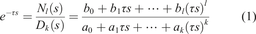
The coefficients of denominator and numerator can be expressed as follows:

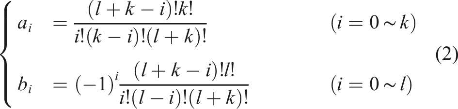
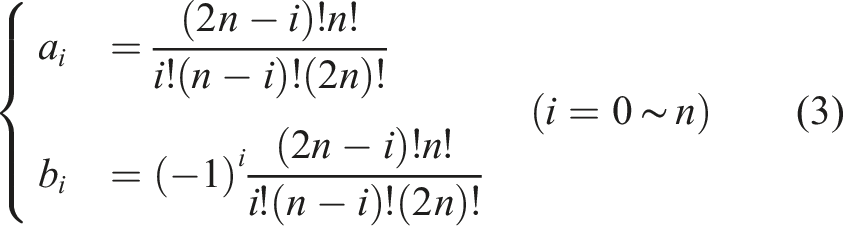
\{\begin{aligned} a_{i} & = \frac{(l + k - i)! k!}{i! (k - i)! (l + k)!} & (i = 0 \sim k) \\ b_{i} & = {(- 1)}^{i} \frac{(l + k - i)! l!}{i! (l - i)! (l + k)!} & (i = 0 \sim l) \end{aligned}

(2)

In engineering applications, to avoid magnitude scaling in the Padé approximation of the time delay term, the numerator and denominator in equation (1) are typically assigned the same order (i.e. l = k = n), thereby yielding an n-th order Padé approximation. The coefficients can be simplified as follows:

\{\begin{aligned} a_{i} & = \frac{(2 n - i)! n!}{i! (n - i)! (2 n)!} \\ b_{i} & = {(- 1)}^{i} \frac{(2 n - i)! n!}{i! (n - i)! (2 n)!} \end{aligned} (i = 0 \sim n)

(3)

2.2. Frequency response characteristics

To assess the accuracy of the Padé approximation, a 100 ms delay is considered. The resulting phase-frequency response is shown in Figure 1(a). For the Padé approximation with equal numerator and denominator orders, the magnitude response remains unity over all frequencies, the corresponding magnitude response curve is omitted in this paper. For the exact time delay element e^−τs, the phase response follows −τω and therefore decreases linearly with increasing angular frequency. In contrast, the Padé approximation exhibits a similar decreasing phase response but with gradual saturation, which is postponed to higher angular frequencies as the approximation order increases, indicating phase errors relative to the exact time delay element.

Figure 1.

Phase response characteristics of Padé approximation: (a) phase-frequency response and (b) error of phase response.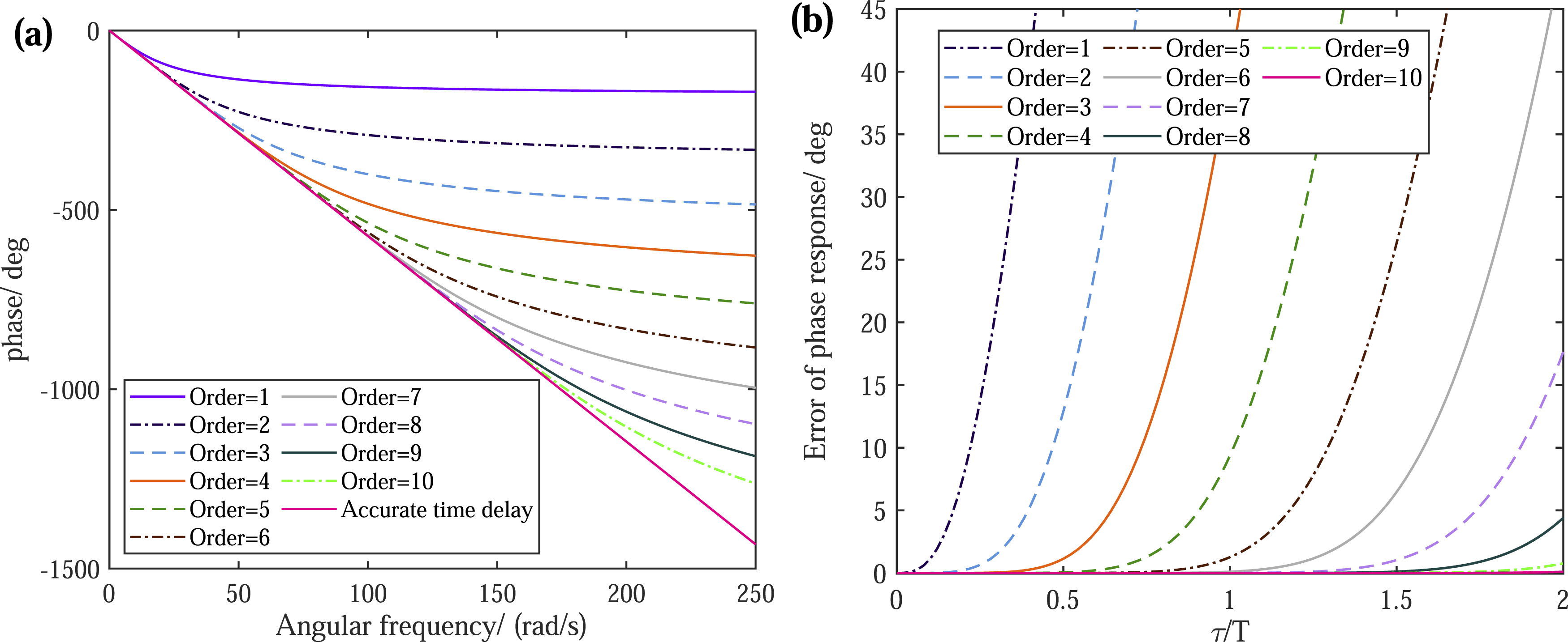

Figure 1(b) presents the phase response errors of the 1st ∼10th-order Padé approximations relative to the exact time delay element, with the horizontal axis expressed in terms of τ/T. Since τ and s appear in equation (1) only as the product τs, the phase error of the Padé approximation can be characterized by a single combined variable. With s = jω and ω expressed in terms of the period T, the ratio τ/T is adopted as the unified variable for the subsequent analysis.

As τ/T increases, the phase error first grows slowly and then more rapidly, showing an overall exponential trend. For a given τ/T, a higher approximation order yields a smaller phase error. Overall, lower approximation orders and higher angular frequencies result in larger phase errors, indicating that higher-order Padé approximations are required to maintain phase accuracy under high-frequency conditions.

2.3. Analysis of required approximation order

Taking a simple harmonic signal as an example, the required order of the Padé approximation for different values of τ/T is analyzed. The approximation accuracy is quantified by the Pearson correlation coefficient (PCC) between the exact delayed signal and the approximated signal, as defined in equation (4).

\begin{aligned} P C C (y_{i}, y_{j}) & = \frac{c o v (y_{i}, y_{j})}{\sqrt{D (y_{i}) D (y_{j})}} \\ = \frac{\sum_{k = 1}^{n} [y_{i} (k) - {\bar{y}}_{i}] [y_{j} (k) - {\bar{y}}_{j}]}{\sqrt{\sum_{k = 1}^{n} {[y_{i} (k) - {\bar{y}}_{i}]}^{2}} \sqrt{\sum_{k = 1}^{n} {[y_{j} (k) - {\bar{y}}_{j}]}^{2}}} \end{aligned}

(4)

where y_i and y_j denote the two time domain signals, and

{\bar{y}}_{i}

and

{\bar{y}}_{j}

denote their mean values.

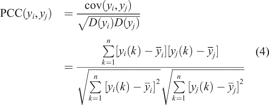
Figure 2 shows that the PCC approaches 1 when τ/T is small and the approximation order is sufficiently high, indicating high approximation accuracy. A threshold of PCC = 0.99 is adopted to ensure sufficient accuracy. The points corresponding to PCC = 0.99 are projected onto the τ/T-order plane in Figure 3. To further quantify the approximation order required under different frequencies and time delays, a linear fit is performed between the required approximation order and τ/T, yielding the relationship Order = 3.631 (τ/T) + 0.421.

Figure 2.

Pearson correlation coefficient (PCC) of time-delayed signals.

Figure 3.

Analysis of required Padé approximation order: (a) required order for PCC = 0.99 and (b) required order versus frequency for τ = 200 ms.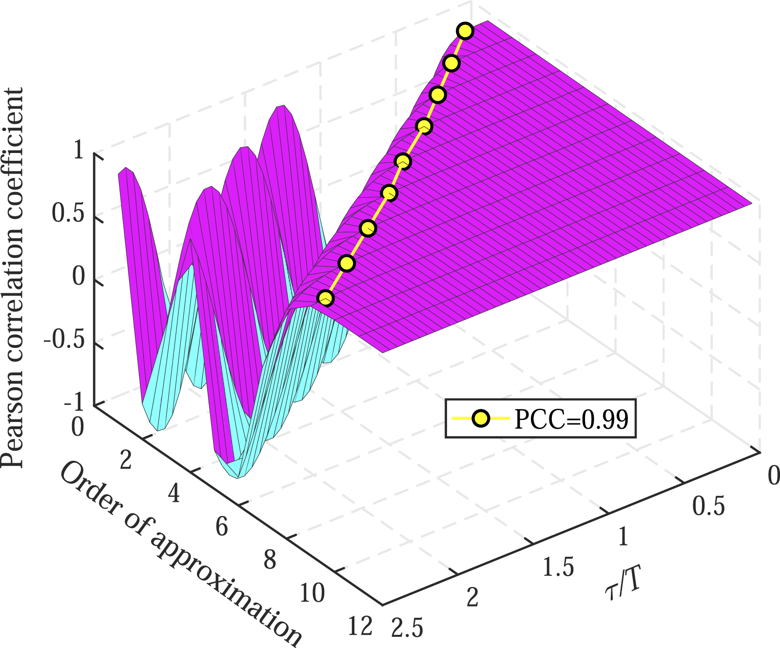

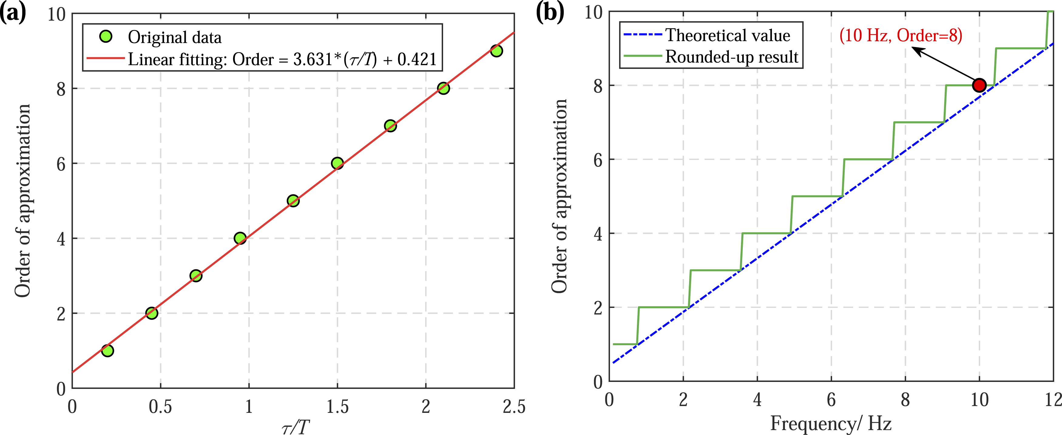
For railway vehicles, the total time delay of active suspension systems is typically below 200 ms (Wu et al., 2023; Shi et al., 2025a). Therefore, τ = 200 ms is taken as a representative case. As shown in Figure 3(b), after rounding the fitted values up to the nearest integer, an 8th-order approximation can ensure PCC $>$ 0.99 at 10 Hz. Since railway vehicle hunting frequencies are generally below 10 Hz and suspension modal frequencies are typically below 2 Hz, the 8th-order approximation is sufficient for the subsequent stability analysis.

3. Dynamics models and active suspension configurations

In this section, a 17-degree-of-freedom (17-DOF) lateral dynamics model and a full-DOF dynamics model are developed, and active suspension control is incorporated into both models. The 17-DOF model is adopted for eigenvalue analysis, whereas the full-DOF model is employed to obtain vibration responses, thereby validating the critical time delay and the corresponding instability characteristics.

3.1. 17-DOF lateral model integrating active control

On the basis of previous work (Chen et al., 2024; Shi et al., 2023), the 17-DOF lateral dynamics model of the whole vehicle integrating secondary active lateral suspension is established. Two active suspension configurations are proposed, as shown in Figure 4, in which the secondary lateral dampers are replaced by actuators, with 2 and 4 actuators installed, respectively. In configuration 1, the passive dampers at the first and fourth positions are replaced by actuators, forming a secondary lateral suspension with parallel active and passive components. In contrast, configuration 2 replaces all lateral dampers with actuators. In the lateral dynamics model, 17 physical DOFs are considered, including the lateral motion y_w,i (i = 1 ∼ 4) and yaw motion ψ_w,i of the four wheelsets, the lateral motion y_f,j, yaw ψ_f,j, and roll φ_f,j (j = 1 ∼ 2) of the two bogies, as well as the lateral motion y_c, yaw ψ_c, and roll φ_c of the carbody. The physical coordinates of the vehicle system are defined as follows:

\begin{aligned} X & = [y_{w 1}, ψ_{w 1}, y_{w 2}, ψ_{w 2}, y_{w 3}, ψ_{w 3}, y_{w 4}, ψ_{w 4}, \\ {y_{f 1}, ψ_{f 1}, φ_{f 1}, y_{f 2}, ψ_{f 2}, φ_{f 2}, y_{c}, ψ_{c}, φ_{c}]}^{T} \end{aligned}

(5)

Figure 4.

Lateral dynamics model integrating active actuators: (a) 2-actuator configuration and (b) 4-actuator configuration.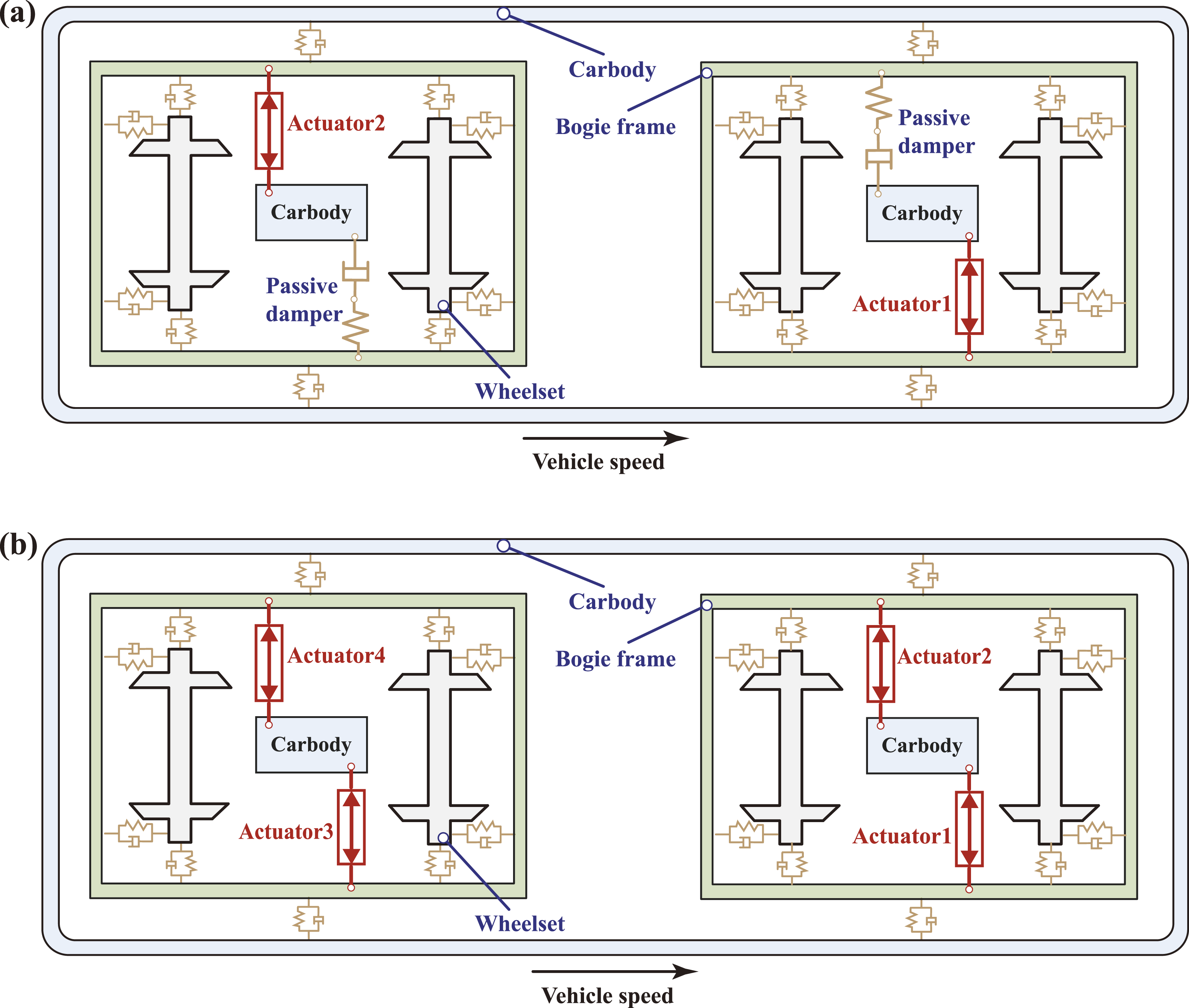

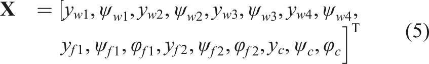
In addition, the anti-yaw dampers and the passive secondary lateral dampers are modelled as Maxwell elements. The corresponding node coordinates y_shd,k, x_yawL,k, and x_yawR,k are also incorporated into the state variables of the vehicle system. In the 17-DOF model, the wheel-rail interaction is linearized, and the creep forces are calculated based on Kalker’s linear theory. For the two suspension configurations, the composition of the state variables in the 17-DOF model is given as follows:

\begin{aligned} Y_{(2)} & = [X^{T}, {\dot{X}}^{T}, y_{shd2}, y_{shd3}, x_{yawL1}, x_{yawR1}, x_{yawL2}, \\ {x_{yawR2}, x_{yawL3}, x_{yawR3}, x_{yawL4}, x_{yawR4}]}^{T} \end{aligned}

(6)

\begin{aligned} Y_{(4)} & = [X^{T}, {\dot{X}}^{T}, x_{yawL1}, x_{yawR1}, x_{yawL2}, x_{yawR2}, \\ {x_{yawL3}, x_{yawR3}, x_{yawL4}, x_{yawR4}]}^{T} \end{aligned}

(7)

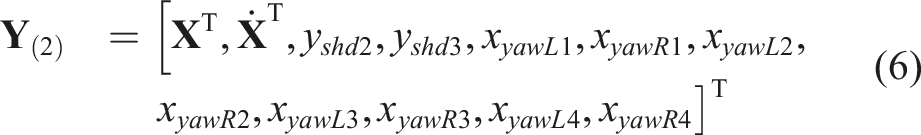
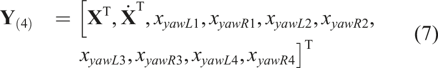
The linearized vehicle system can be expressed as follows:

\dot{Y} = A Y + B U

(8)

where Y and

\dot{Y}

denote the state variables of the vehicle system and their derivatives, respectively.

For the two active suspension configurations, the matrices of the actual control forces are as follows:

U_{(2)} = {[F_{a, 1}, F_{a, 4}]}^{T}

(9)

U_{(4)} = {[F_{a, 1}, F_{a, 2}, F_{a, 3}, F_{a, 4}]}^{T}

(10)

When the time-delayed control force is handled using the Padé approximation, the time delay of each control force is treated as an independent variable. Consequently, the input dimension of the corresponding Padé approximation block is 2 and 4 for the two active suspension configurations, respectively. The input matrices under the two active suspension configurations are provided in Appendix 1.

3.2. Full-DOF dynamics model and co-simulation workflow

A three-dimensional multibody dynamics model of the whole vehicle is developed in SIMPACK, hereinafter referred to as the full-DOF model. The vehicle system is characterized by 50 DOFs, incorporating nonlinearities such as wheel-rail contact relationship and damper unloading characteristics. The new LMB wheel profile and the CN60 rail profile were adopted, resulting in an equivalent wheel-rail conicity of 0.17.

On the other hand, the controller is implemented in Simulink to calculate the feedback control forces, and the time delay in the active suspension system is modelled using the Transport Delay block. The Simat interface is adopted for data exchange between the vehicle dynamics model and the controller, including state feedback variables and active control forces, thereby enabling co-simulation of the vehicle-active suspension control system. Due to the output force limitation of the actuator, the upper saturation limit of the control force is set to 30 kN. The simulation procedure of the vehicle-active suspension control system is shown in Figure 5.

Figure 5.

Co-simulation workflow of the vehicle-active suspension control system.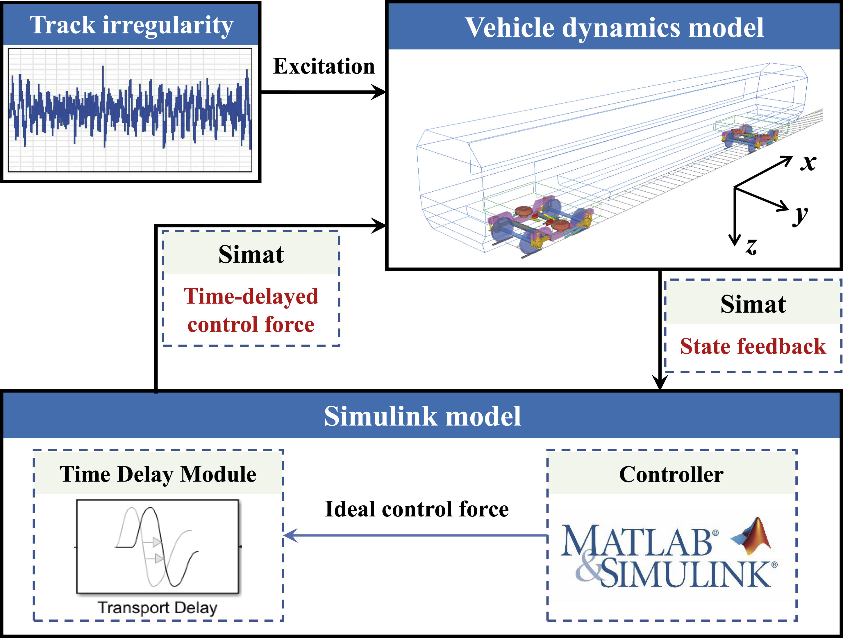

4. Stability analysis method and its verification

4.1. Stability analysis method for the time-delayed feedback control system

For the time delay element, the Padé approximation can be converted from its transfer function into the state-space equations, which are given as follows:

\dot{G} = A_{g} G + B_{g} U_{0}

(11)

U = C_{g} G + D_{g} U_{0}

(12)

where G is a column vector composed of time delay intermediate variables. For each independent time delay term, the intermediate variables of the n-th order Padé approximation are of dimension n. U₀ denotes the original input vector without time delay. If there are m independent signals to be processed by the delay element, the input vector is m-dimensional. U denotes the output vector of the time delay system obtained by Padé approximation. A_g, B_g, C_g, and D_g denote the state matrix, input matrix, output matrix, and direct feedthrough matrix derived from the transfer function, with dimensions (mn) × (mn), (mn) × m, m × (mn), and m × m, respectively.

Substituting the time-delayed signal U obtained from equation (12) into equation (8) yields:

\dot{Y} = A Y + B C_{g} G + B D_{g} U_{0}

(13)

For linear feedback control, the ideal control force without time delay can be expressed as:

U_{0} = - K_{f} Y

(14)

For the vehicle system investigated in this study, the expressions of matrices B, U, and K_f are provided in Appendix 1. Substituting equation (14) into Equations (13) and (11) yields the expression for the coupled system consisting of the vehicle dynamics and the time delay element as follows:

\{\begin{aligned} \dot{Y} & = (A - B D_{g} K_{f}) Y + B C_{g} G \\ \dot{G} & = A_{g} G - B_{g} K_{f} Y \end{aligned}

(15)

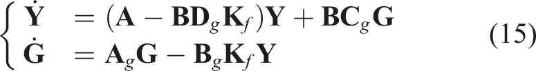
Subsequently, time delay intermediate variables are incorporated into the state variables of the vehicle system to form a new state vector $Z = {[Y^{T} G^{T}]}^{T}$ . The vehicle system with time-delayed feedback control can then be written in concise form as follows:

\dot{Z} = A_{z} Z

(16)

where A_z denotes the state matrix of the vehicle system with time-delayed feedback control, which can be expressed in block matrix form as follows:

A_{z} = [\begin{matrix} A - B D_{g} K_{f} & B C_{g} \\ - B_{g} K_{f} & A_{g} \end{matrix}]

(17)

As seen from equation (17), the block matrix includes matrix A describing the inherent characteristics of the vehicle system, matrix B associated with the control input, and the feedback control matrix K_f. In addition, A_g, B_g, C_g, and D_g corresponding to time delay element are all considered in the formulation of A_z. Therefore, the vehicle system with state feedback control and the time delay element modelled using Padé approximation are integrated into a coupled unified system. In the subsequent analysis, the stability of the system can be determined from the eigenvalues of the state matrix A_z.

To determine the eigenvalues and eigenvectors of the state matrix A_z, and thus obtain the modal frequencies and damping ratios of the vehicle system, the general solution Z = Z₀e^ηt of the differential equation is substituted into equation (16), yielding

(A_{z} - η I) Z_{0} = 0

(18)

where η denotes the eigenvalues of the system and Z₀ represents the matrix composed of eigenvectors.

To ensure a nontrivial solution for Z₀, the characteristic equation is given by

\det (A_{z} - η I) = 0

(19)

Solving the determinant yields n′ pairs of complex conjugate roots:

η_{i} = α_{i} \pm j β_{i} (i = 1 \sim n^{'})

(20)

For the vehicle system with time-delayed feedback control, the system order n′ is the sum of the number of vehicle state variables and the intermediate variables introduced by the Padé approximation.

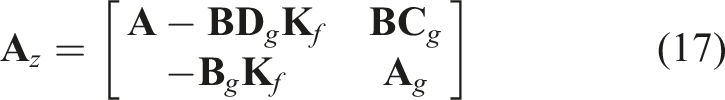
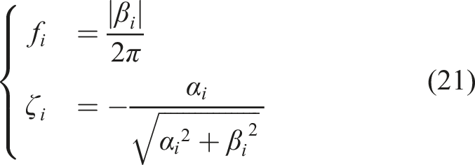
The modal frequencies and damping ratios can be calculated as follows:

\{\begin{aligned} f_{i} & = \frac{| β_{i} |}{2 π} \\ ζ_{i} & = - \frac{α_{i}}{\sqrt{{α_{i}}^{2} + {β_{i}}^{2}}} \end{aligned}

(21)

Substituting equation (20) into equation (18) yields the complex eigenvectors as follows:

Z_{0}^{(i)} = {[{(X_{0}^{(i)})}^{T} {(η_{i} X_{0}^{(i)})}^{T} {(X_{D}^{(i)})}^{T} {(G_{0}^{(i)})}^{T}]}^{T}

(22)

where

X_{0}^{(i)}

denotes the displacements in physical coordinate of the vehicle system contained in the complex eigenvector. h represents the number of physical coordinates of the vehicle model; h = 17 for the 17-DOF lateral dynamics model and h = 50 for the full-DOF model.

X_{D}^{(i)}

corresponds to the node coordinates of the Maxwell model.

G_{0}^{(i)}

represents the time delay intermediate variable, which lacks direct physical meaning.

4.2. Method verification based on 1-DOF system

Taking the 1-DOF system as an example, the correctness of the aforementioned stability analysis method is verified. Since exact eigenvalues of delay differential equations are difficult to obtain analytically, the results obtained from DDE-BIFTOOL (Engelborghs et al., 2002) are used as the reference for comparison with those derived via the Padé approximation.

The 1-DOF system with time delay is shown in Figure 6. The system consists of a mass m₁, a stiffness term k₁ and a damping term c₁ without delay, as well as a linear feedback control term $u_{1} = - c_{s} {\dot{x}}_{1} (t - τ)$ , with time delay τ. The 1-DOF system is parameterized with an undamped natural frequency of 10 Hz and a damping ratio of 0.2, and the delayed damping coefficient is defined as c_s = 2c₁. With the parameters listed in Table 1, the dynamics equation of the system is governed as follows:

m_{1} {\ddot{x}}_{1} (t) + c_{1} {\dot{x}}_{1} (t) + c_{s} {\dot{x}}_{1} (t - τ) + k_{1} x_{1} (t) = 0

(23)

Figure 6.

1-DOF system with time-delayed feedback control.

Table 1.

Parameters of the 1-DOF system.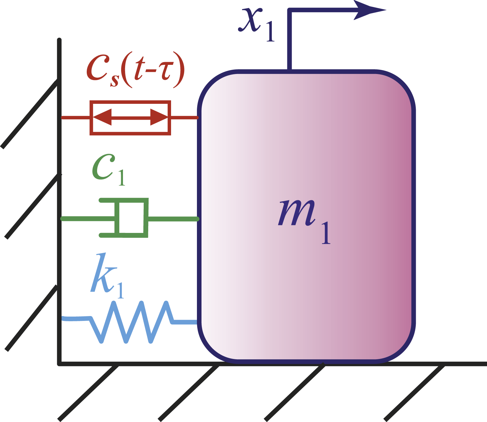

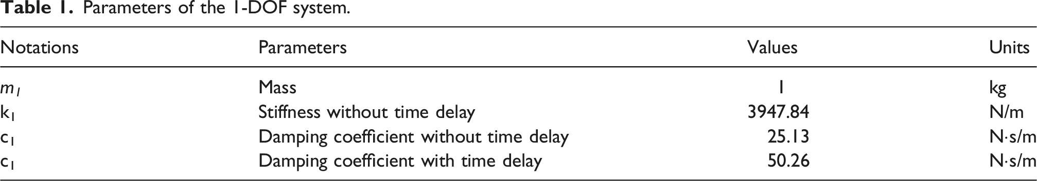
Notations	Parameters	Values	Units
m₁	Mass	1	kg
k₁	Stiffness without time delay	3947.84	N/m
c₁	Damping coefficient without time delay	25.13	N⋅s/m
c₁	Damping coefficient with time delay	50.26	N⋅s/m

The stability analysis method presented in Section 4.1 is applied to the 1-DOF system, with the time delay ranging from 2 to 250 ms. The results are shown in Figure 7, where the scatter points are spaced at 2 ms intervals, and the marker size increases linearly with the time delay. The red ‘+’ symbols denote the results obtained via DDE-BIFTOOL, while the other symbols represent the results from Padé approximations of different orders, respectively. As shown in Figure 7(a), the first-order approximation exhibits substantial errors. When the time delay exceeds 6 ms, the eigenvalues rapidly deviate from those obtained using DDE-BIFTOOL and higher-order approximations. As the time delay exceeds 30 ms, deviations become apparent in the second-order approximation. However, the amplitude of the deviation remains smaller than that of the first-order approximation. Figure 7(b) presents a magnified view for large time delays (184 ∼250 ms). It can be observed that the fourth-order approximation yields relatively small approximation errors relative to DDE-BIFTOOL benchmark.

Figure 7.

Root locus diagram of the 1-DOF system: (a) overall view and (b) local enlarged view.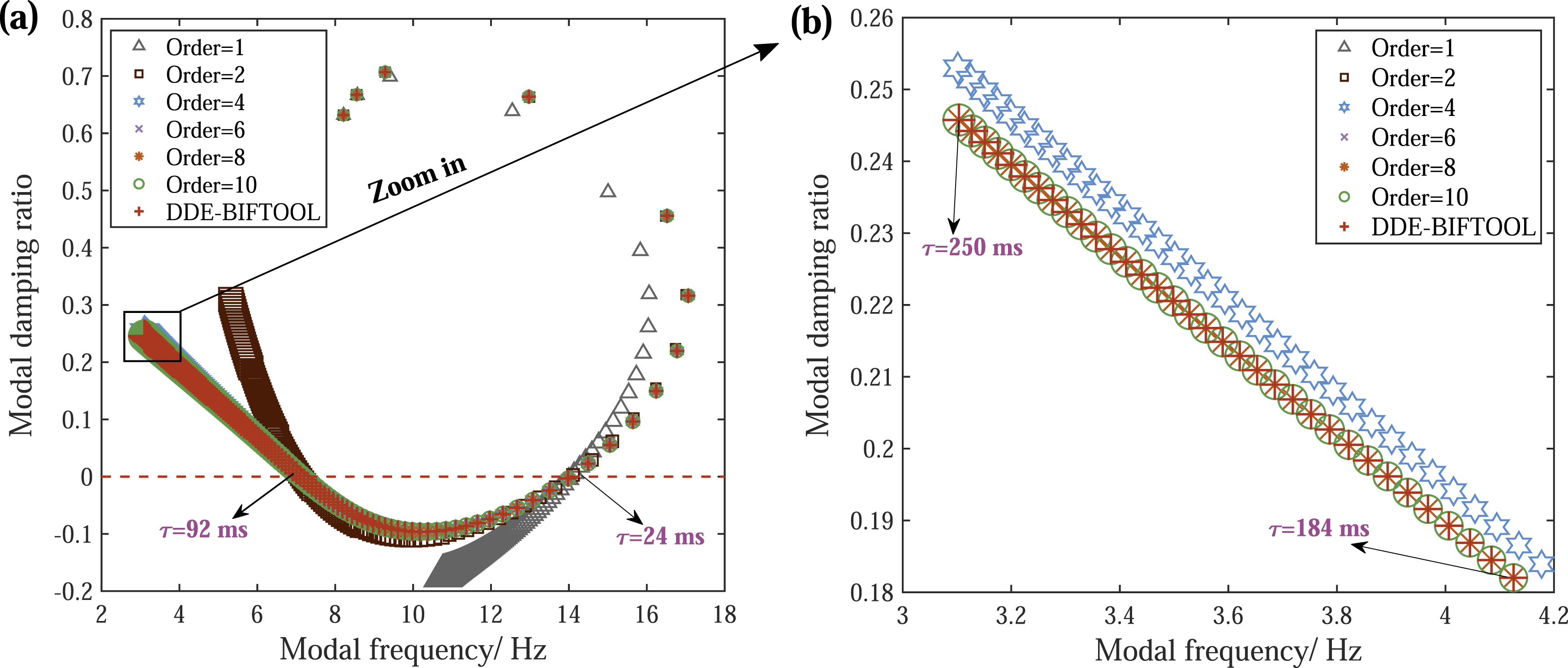

The errors of the Padé approximation relative to DDE-BIFTOOL are subsequently analyzed in terms of modal frequency and damping ratio. The corresponding errors under different approximation orders and time delays are illustrated in Figure 8. Figure 8(a) presents the absolute values of the relative errors in modal frequency. Within the time delay range of 0 ∼250 ms, the relative errors of the 4 ∼8th order approximations remain below 1%. Figure 8(b) shows the absolute errors of the modal damping ratio. Within the considered range, the errors associated with the 5th and higher order approximations are nearly negligible.

Figure 8.

Estimation error of modal parameters under different approximation orders and time delays: (a) relative error of modal frequency and (b) absolute error of damping ratio.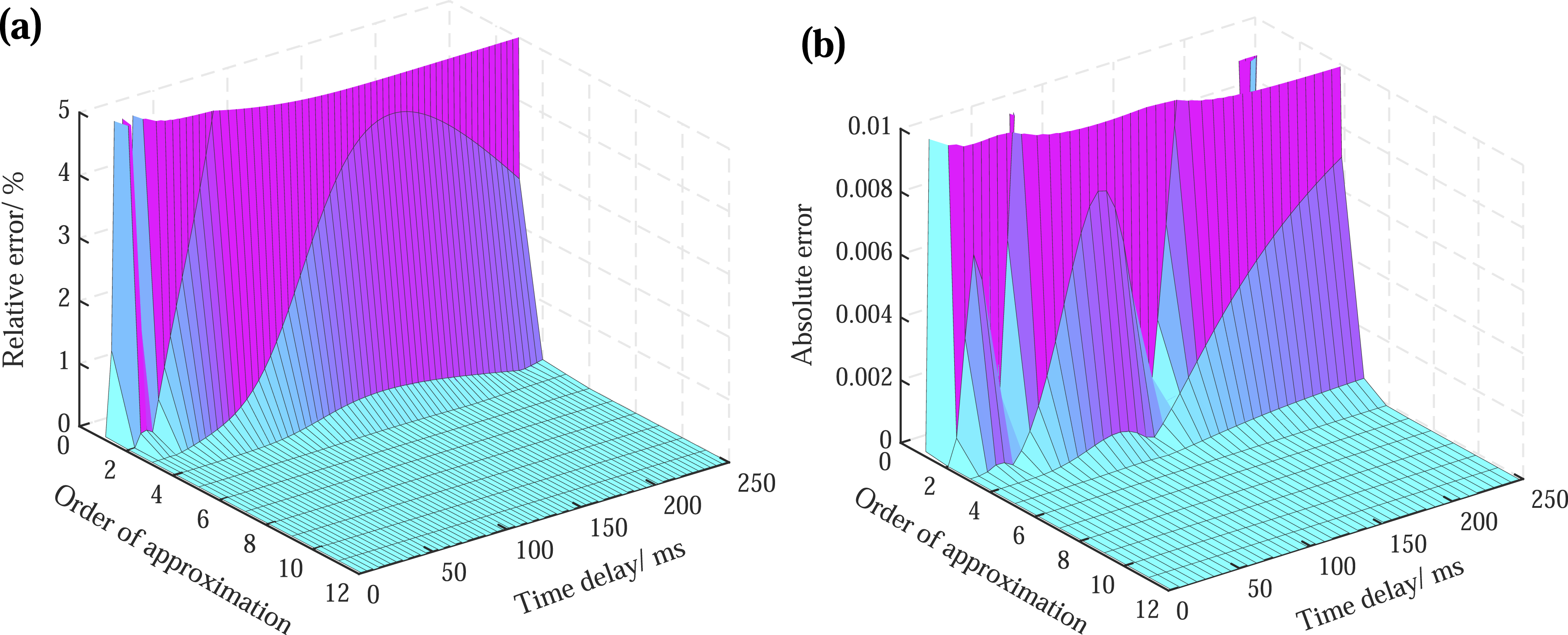

5. Stability analysis of vehicle system with time-delayed sky-hook damping control

In this section, the full-active sky-hook damping strategy is applied to the active lateral suspension system of railway vehicles. For sky-hook damping control, the feedback control force is linearly related to the lateral velocity of carbody v, as expressed by F_A = −c_skyv, where c_sky is the damping coefficient.

5.1. Abrupt instability induced by time delay

Based on the co-simulation of the vehicle-active suspension system, the effects of time delay on lateral Sperling index and bogie lateral acceleration are investigated at a vehicle speed of 300 km/h under different sky-hook damping coefficients. The results under the 4-actuator configuration are shown in Figure 9. As shown in Figure 9(a), a sharp increase in the lateral Sperling index is observed as the time delay increases. On the other hand, the root-mean-square (RMS) of the bogie lateral acceleration in Figure 9(b) also exhibits an abrupt jump. The time delay associated with this jump coincides with that at which the Sperling index exhibits a sharp increase, indicating that the carbody and the bogie lose stability almost simultaneously. It can be seen that once the time delay exceeds a certain threshold, the vehicle system will undergo a sudden and severe instability, posing a serious threat to operational safety. Therefore, it is necessary to adopt the stability analysis method proposed in Section 4.1 to quantify the critical time delay that leads to severe instability of the vehicle-active suspension system.

Figure 9.

The influence of time delay on dynamic performance indices: (a) lateral Sperling index and (b) bogie lateral acceleration.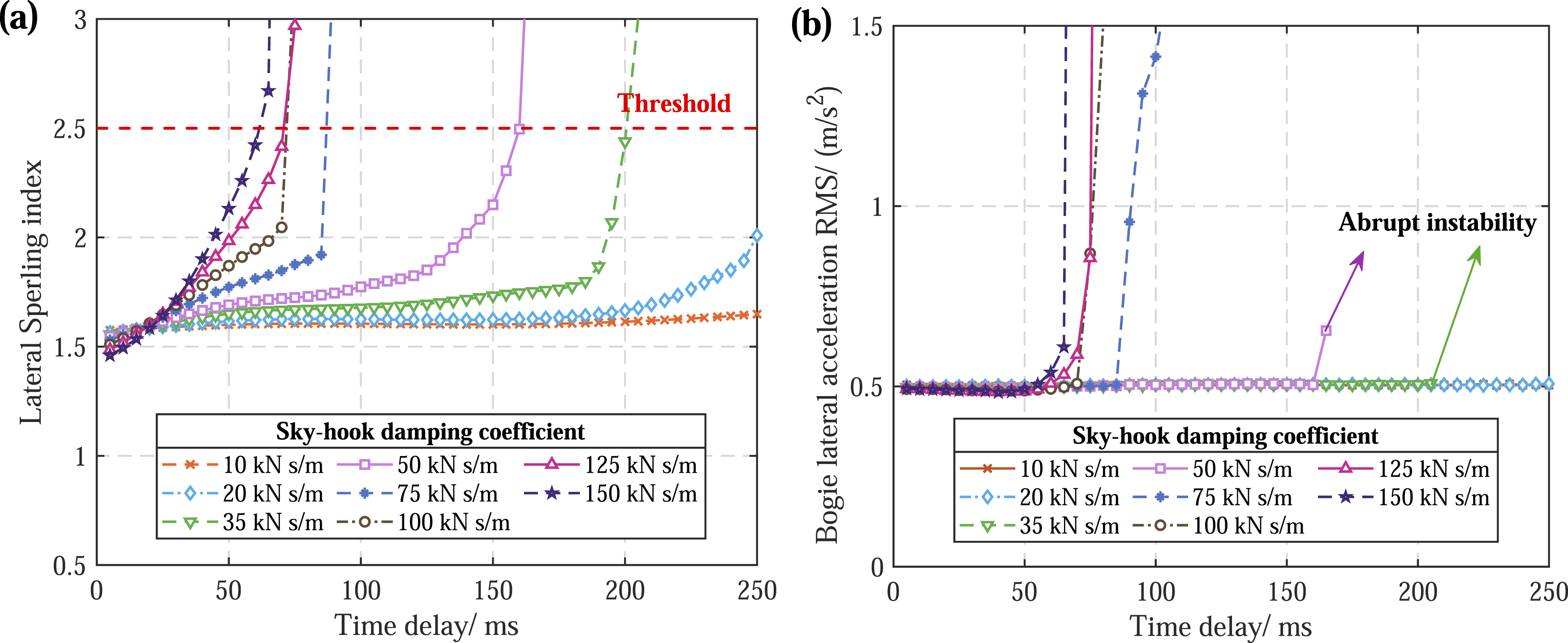

5.2. Determination of the critical time delay for instability

Taking c_sky = 35 kN ⋅ s/m under the 4-actuator configuration as an example, the variation of the system eigenvalues with the feedback control time delay is investigated. The analysis is performed for the time delay range of 2 ∼250 ms, with a step size of 2 ms. The root locus diagram obtained from the 17-DOF model is shown in Figure 10. The eigenvalue results obtained from the linearized full-DOF model show good agreement with those of the 17-DOF model. Therefore, the detailed results are omitted in this paper.

Figure 10.

Root loci of the vehicle system with time-delayed active suspension control obtained by the 17-DOF model.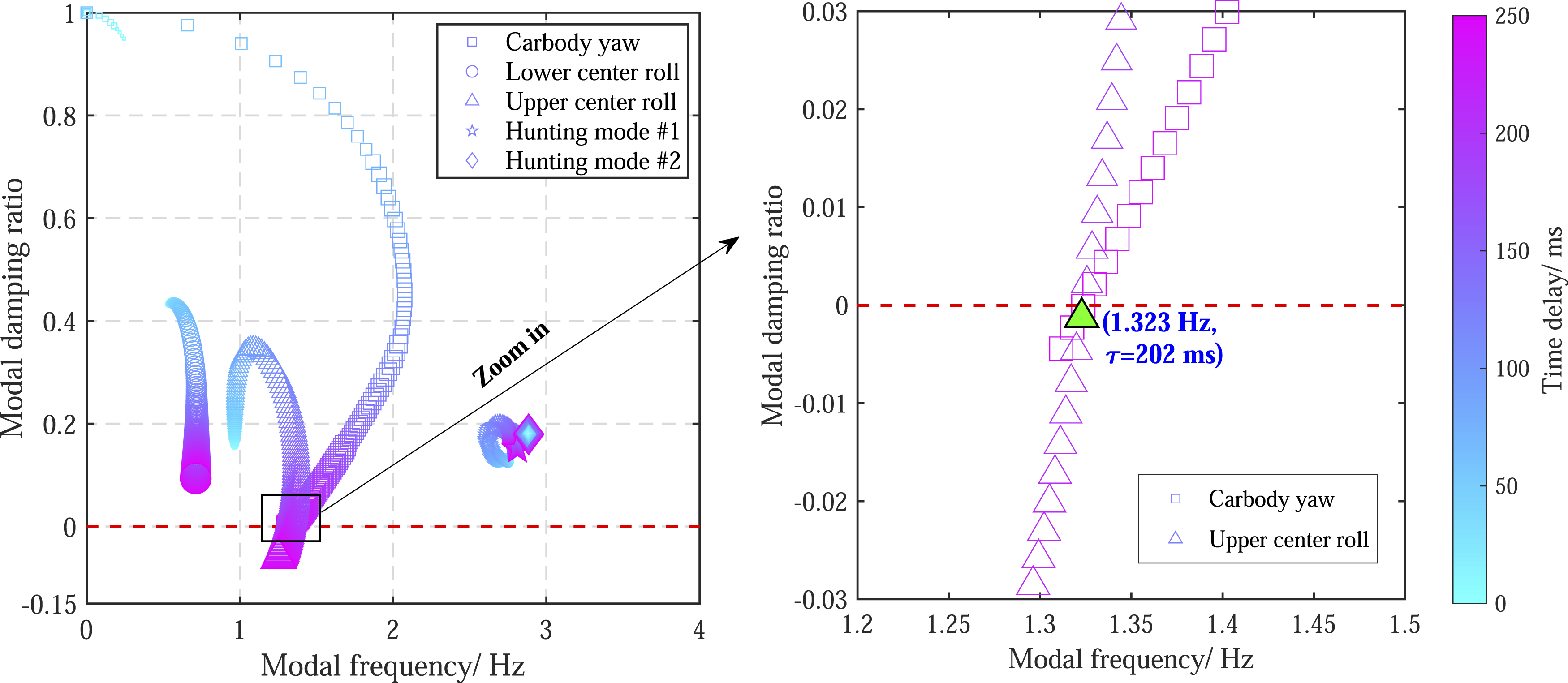

In Figure 10, only the hunting modes and the carbody suspension modes are presented. As the time delay increases, the damping ratios of the carbody suspension modes show an overall decreasing trend, indicating a progressive reduction in the stability margin of the suspension modes and a corresponding increase in the risk of instability. Furthermore, the hunting modes exhibit only minor variations with increasing time delay, and no delay-induced instability is observed in these modes. From the stability perspective, as the time delay increases, the damping ratios of certain carbody suspension modes decrease below zero, and the first mode whose damping ratio becomes negative determines the stability. Based on the root locus method, with the zero-crossing of the minimum damping ratio adopted as the instability threshold, the critical time delay for instability can be regarded as approximately 202 ms from the eigenvalue perspective, with a corresponding unstable modal frequency of 1.323 Hz.

5.3. Verification of the critical time delay for instability

Subsequently, the critical time delay for instability is verified via co-simulation of the vehicle-active suspension system. A section of track irregularity is applied as the initial excitation and removed before 10 s, and the vibration response of the vehicle system is analyzed. The lateral accelerations at the front and rear floor of the carbody are presented in Figure 11(a) and (b), respectively. For the time delay of τ = 195 ms, the amplitude of carbody lateral acceleration decreases progressively, indicating the system is stable. At τ = 197 ms, sustained oscillations are observed, corresponding to the critical state of instability. When τ = 200 ms, the carbody acceleration diverges, indicating loss of stability.

Figure 11.

Time histories of carbody lateral acceleration without track irregularity: (a) front of carbody and (b) rear of carbody.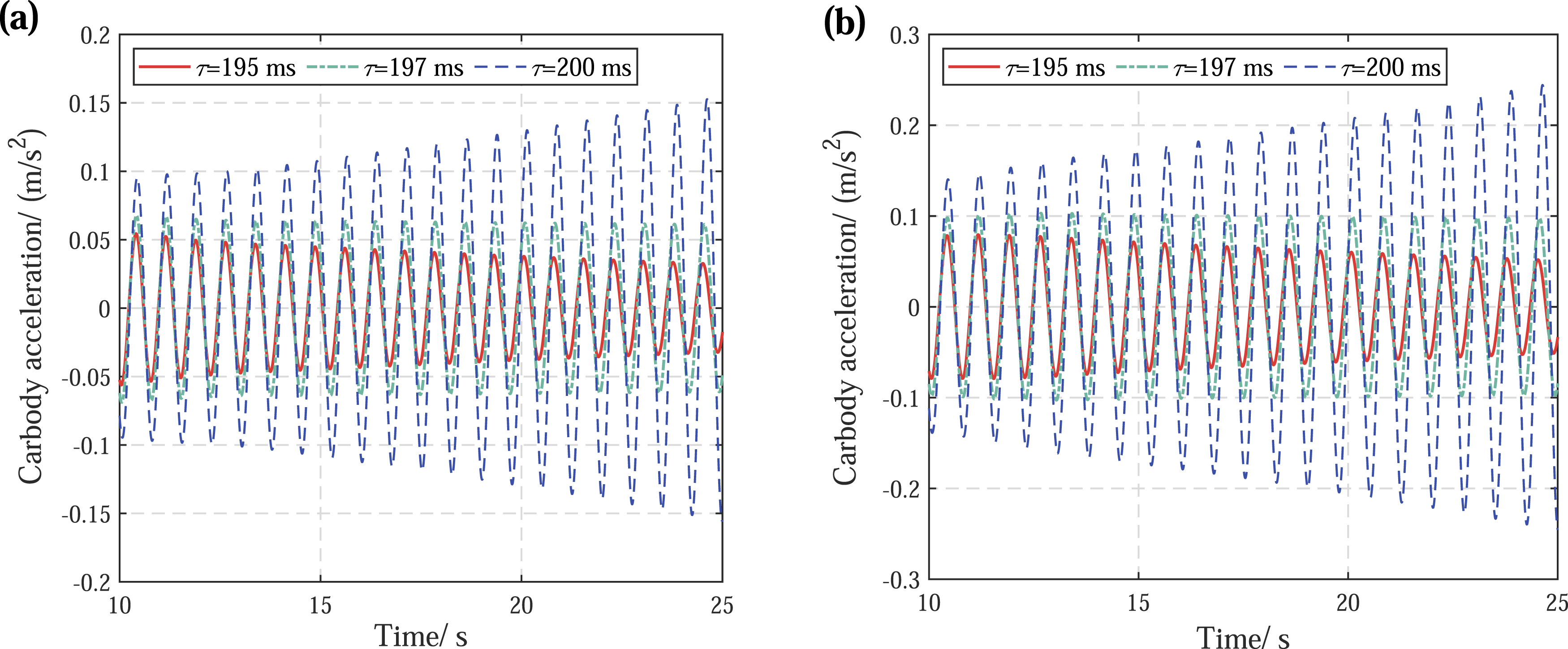

The time domain results presented in Figure 11 indicate that the critical time delay for instability of the vehicle system is approximately 197 ms. This estimate can be further corroborated from two complementary perspectives, namely, the abrupt variation in dynamic performance indices and the root locus analysis. Specifically, the root locus analysis in Figure 10 yields a closely comparable critical value of approximately 202 ms. Moreover, as shown in Figure 9, the performance indices exhibit a pronounced jump as the time delay approaches 200 ms for the 4-actuator configuration with c_sky = 35 kN ⋅ s/m, providing additional evidence for the onset of instability. Therefore, by taking the time domain simulation as the primary stability criterion and using the root locus method and performance index evaluation as supporting evidence, the critical time delay for instability is determined to be 197 ms.

5.4. Analysis of instability mode shape

A time-delay case of τ = 205 ms, slightly above the critical time delay, is selected to analyze the mode shape characteristics of the first unstable mode. The polar diagram obtained from the full-DOF model is illustrated in Figure 12. Figure 12 shows that the mode shape is predominantly characterized by the lateral and roll motion of carbody. In Figure 12, the carbody lateral motion and roll are nearly out of phase, which is consistent with the modal characteristics of the upper centre roll mode.

Figure 12.

Mode shape of the unstable mode at τ = 205 ms.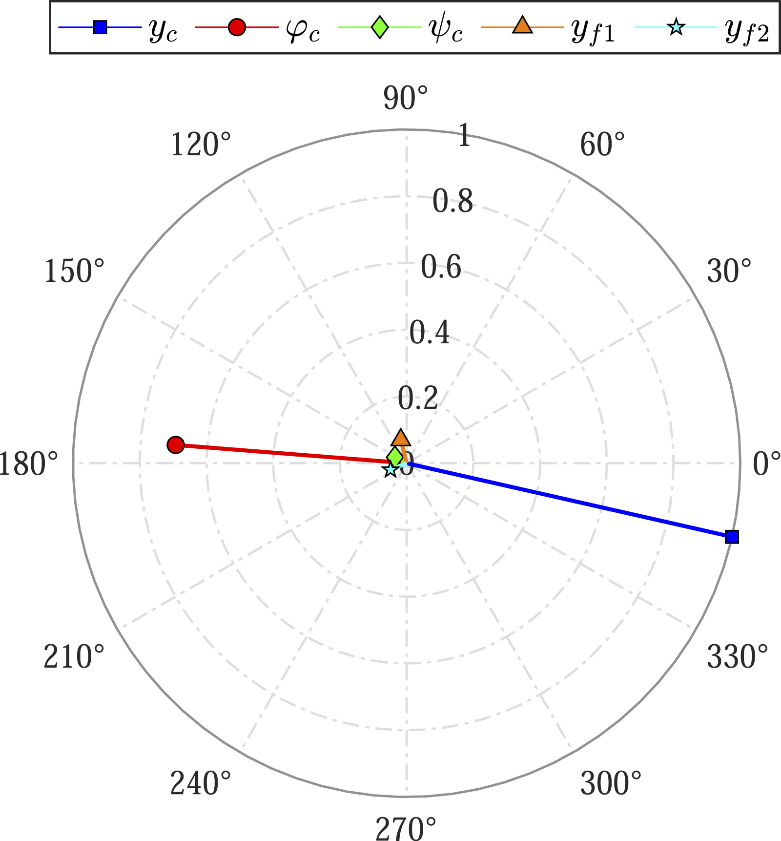

Furthermore, the vibration characteristics of the vehicle system under unstable conditions are verified. For the time delay of τ = 205 ms, the WG50 spectrum is applied as track irregularity. The time domain response and corresponding frequency domain response of the carbody lateral accelerations are shown in Figure 13(a) and (b), respectively. As shown in Figure 13(a), the lateral accelerations at the front and rear of the carbody exhibit divergent harmonic vibrations with a dominant frequency of 1.33 Hz and nearly in-phase characteristics. These features are consistent with those of the upper centre roll mode in the full-DOF model.

Figure 13.

Carbody lateral acceleration at τ = 205 ms: (a) time domain and (b) frequency domain.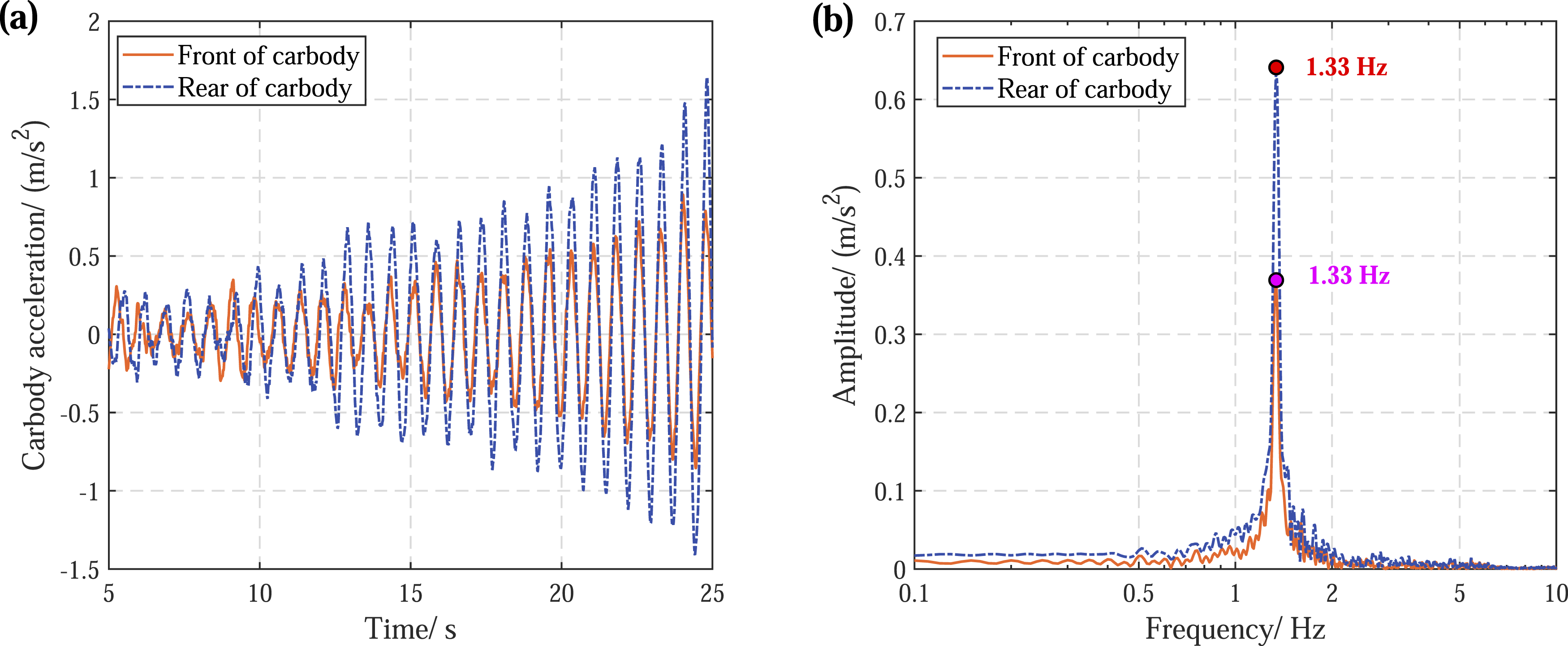

5.5. Influence of damping coefficient and suspension configuration

As shown in Figure 9, the critical time delay corresponding to the abrupt instability of the vehicle system varies significantly under different sky-hook damping coefficients. The time delays corresponding to abrupt jumps in performance indices are listed in Table 2. When the 2-actuator configuration is adopted and the damping coefficient is relatively small, no abrupt instability is observed within the investigated time delay range of 0 ∼250 ms. For the remaining conditions, both lateral Sperling index and bogie lateral acceleration increase sharply due to the abrupt instability of the system. The results in Table 2 indicate that an increase in the sky-hook damping coefficient leads to a reduction in the critical time delay.

Table 2.

Time delays at jump points of performance indices.

Sky-hook damping coefficient/(kN⋅ s/m)	Time delay/ms
Sky-hook damping coefficient/(kN⋅ s/m)	2-actuator configuration	4-actuator configuration
35	—	200
50	—	160
75	230	90
100	160	75
125	90	75
150	75	65
200	65	—

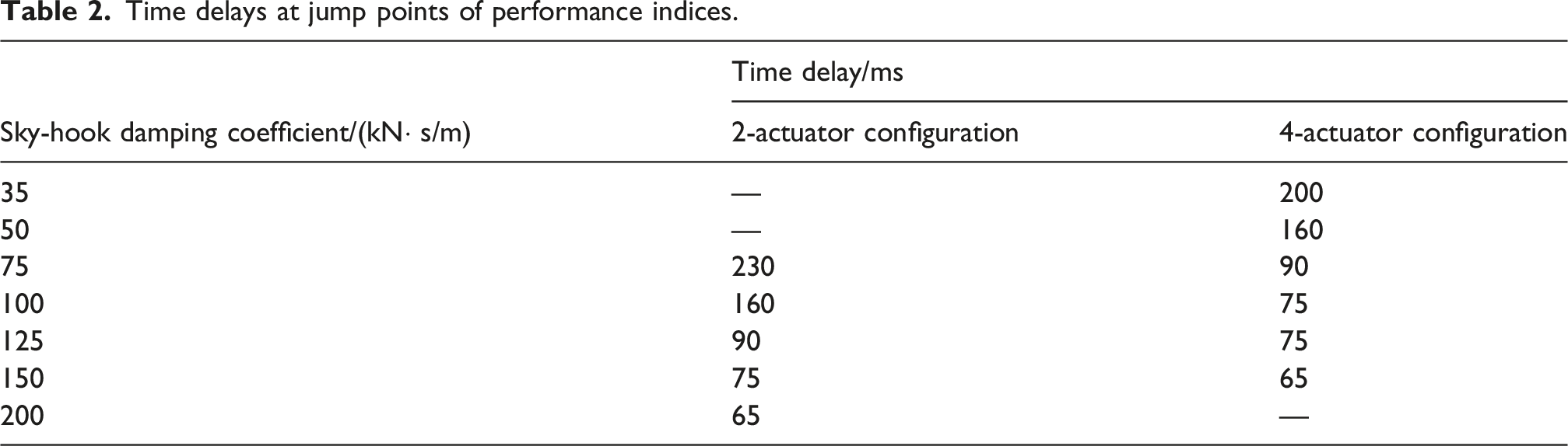
The comparison between the time delays obtained by the eigenvalue method and those corresponding to the abrupt jumps in the performance indices is shown in Figure 14(a). Overall, the critical time delays obtained from the eigenvalue method are essentially consistent with those determined from the jump points of the performance indices. When the same sky-hook damping coefficient is adopted, the 4-actuator configuration generates larger control forces than the 2-actuator configuration, leading to a stronger damping effect. As demonstrated in prior work (Ji et al., 2025), a higher inherent damping without time delay and a lower time-delayed adjustable damping in the system are beneficial for increasing the critical time delay. For the 2-actuator configuration, the passive lateral dampers retained in the suspension provide certain inherent damping, thereby reducing the relative proportion of time-delayed adjustable damping in the vehicle system. Under the same sky-hook damping coefficient, the 2-actuator configuration exhibits a lower time-delayed adjustable damping while simultaneously providing a higher inherent damping compared with the 4-actuator configuration. Consequently, the 2-actuator configuration achieves a higher critical time delay than the 4-actuator configuration. Regarding the maximum allowable time delay for maintaining system stability, the sky-hook damping coefficient should not be excessively high.

Figure 14.

The influence of sky-hook damping coefficient on instability characteristics: (a) critical time delay and (b) instability frequency.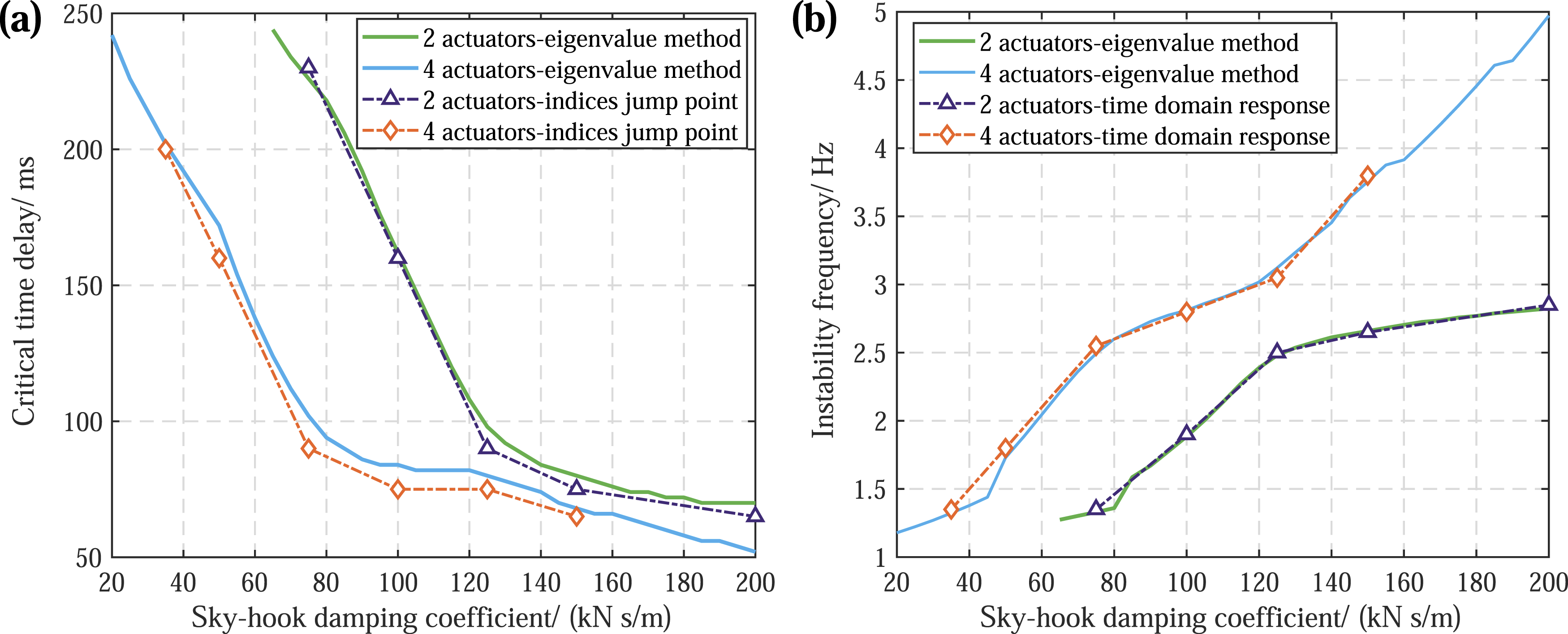

Under certain conditions, the time delays corresponding to the abrupt jumps in performance indices of the vehicle system are slightly lower than the critical time delays determined from the eigenvalue method. In engineering applications, when an eigenvalue-based linear stability analysis is employed, a damping ratio threshold of 5%, which is commonly adopted in engineering practice, can be used as the stability criterion to ensure an adequate stability margin for time-delayed feedback control systems.

On the other hand, the instability frequencies corresponding to the critical time delays are shown in Figure 14(b). The solid lines denote the modal frequencies obtained by the eigenvalue method, while the scatter points connected by dash-dotted lines represent the dominant frequencies of the carbody lateral acceleration under WG50 track irregularity excitation. The theoretical instability frequencies derived from the eigenvalue method show good agreement with those obtained by time domain response, and the instability frequency increases with increasing sky-hook damping coefficient.

The relationship between the critical time delay and the corresponding instability frequency is further investigated, as shown in Figure 15. Figure 15(a) shows a two-dimensional scatter plot of the critical time delay and the instability frequency, with the marker size representing the sky-hook damping coefficient. A clear inverse relationship is observed between the critical time delay and the instability frequency: For both suspension configurations, a larger critical time delay is associated with a lower instability frequency. As shown in Figure 15(b), the product of the critical time delay and the corresponding instability frequency exhibits only minor variation with the sky-hook damping coefficient and remains approximately around 0.25.

Figure 15.

Relationship between the critical time delay and corresponding instability frequency: (a) critical time delay versus instability frequency and (b) product of critical time delay and corresponding instability frequency.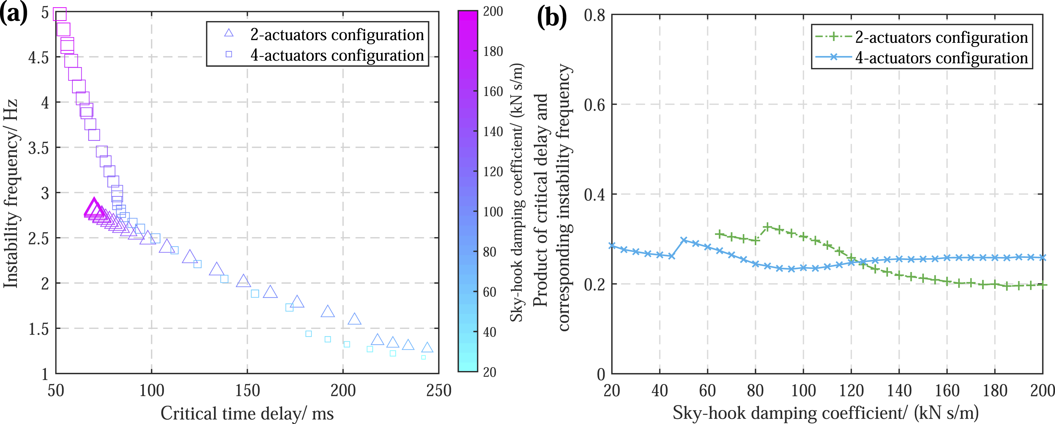

6. Conclusions and prospects

To investigate the instability problem of the vehicle-active suspension control system induced by time delay, a stability analysis method for time-delayed feedback control systems based on Padé approximation is proposed, followed by verification of the accuracy in eigenvalue calculation. Taking the sky-hook damping strategy as an example, the influence mechanism of feedback control time delay on system stability is investigated from the perspective of system eigenvalues, and the theoretical results are validated through co-simulation. The main conclusions are as follows:

(1) When the numerator and denominator are of the same order, the Padé approximation preserves the signal amplitude while introducing a phase error, which increases as the approximation order decreases and τ/T increases. For frequencies below 10 Hz and time delays below 200 ms, an 8th-order approximation is sufficiently accurate, maintaining a PCC above 0.99.

(2) Analysis of the 1-DOF system demonstrates that for sufficiently high approximation orders, the eigenvalues obtained by the Padé approximation method exhibit small deviations in both modal frequency and damping ratio compared with those derived from DDE-BIFTOOL, indicating that the proposed method can achieve accurate eigenvalue computation.

(3) For active sky-hook damping control, if the time delay exceeds a critical threshold, the system exhibits abrupt and severe instability. Both the lateral Sperling index and the bogie lateral acceleration undergo a sudden jump. Under different active suspension configurations and sky-hook damping coefficients, the time delays corresponding to the abrupt jump in the performance indices are in good agreement with the critical time delays at which the minimum damping ratio reaches zero, which verifies the validity of the proposed stability analysis method.

(4) Considering the 4-actuator configuration with a sky-hook damping coefficient of c_sky = 35 kN ⋅ s/m, the carbody upper centre roll mode undergoes instability first as the time delay increases, with its damping ratio decreasing below zero prior to that of the other modes. Time domain analysis indicates that the critical time delay for instability is approximately 197 ms. At the onset of instability, the carbody lateral acceleration is dominated by a single frequency component that coincides with the frequency of the unstable mode. The phase relationship between the front and rear sensors of the carbody is in accordance with the characteristics of the upper centre roll mode.

(5) As the sky-hook damping coefficient increases, the maximum allowable time delay for ensuring system stability decreases. For the same sky-hook damping coefficient, the critical time delay for instability of the 2-actuator configuration is significantly higher than that of the 4-actuator configuration. To improve the time delay robustness of the railway vehicle system with sky-hook damping control, a smaller sky-hook damping coefficient and the 2-actuator configuration are recommended.

In future work, the proposed stability analysis framework can be further extended to additional linear feedback control strategies, such as ground-hook damping control, sky-hook and ground-hook mixed control, and Linear Quadratic Regulator (LQR) control. The critical time delay for instability under different control laws can then be quantitatively evaluated, thereby providing practical insights for engineering applications of active suspension systems. For semi-active control strategies with state-switching criteria, linearization methods for the switching criteria can be further investigated. On this basis, the time delay adaptability of such strategies can be systematically analyzed. In addition, further work may build on the present study by investigating delay prediction and compensation for active suspension systems, and by analyzing the stability of the compensated vehicle system.

Footnotes

ORCID iDs

Longfei Chen

Huailong Shi

Funding

The authors disclosed receipt of the following financial support for the research, authorship, and/or publication of this article: This work was supported by the National Natural Science Foundation of China [Grant Numbers 52272406, U2468227] and the Sichuan Science and Technology Project [Grant Numbers 2025ZNSFSC0034, 2025ZNSFSC0398].

Declaration of conflicting interests

The authors declare that they have no known competing financial interests or personal relationships that could have appeared to influence the work reported in this paper.

Matrices of vehicle-active suspension control system

The input matrices of the two suspension configurations are given as follows: (A1-1)

B_{(2)} = {[\begin{matrix} 0_{1 \times 25} & \frac{1}{m_{f}} & \frac{L_{d}}{I_{f z}} & \frac{h_{6}}{I_{f x}} & 0 & 0 & 0 & - \frac{1}{m_{c}} & \frac{- L_{c} - L_{d}}{I_{c z}} & - \frac{h_{5}}{I_{c x}} & 0_{1 \times 10} \\ 0_{1 \times 25} & 0 & 0 & 0 & \frac{1}{m_{f}} & - \frac{L_{d}}{I_{f z}} & \frac{h_{6}}{I_{f x}} & - \frac{1}{m_{c}} & \frac{L_{c} + L_{d}}{I_{c z}} & - \frac{h_{5}}{I_{c x}} & 0_{1 \times 10} \end{matrix}]}^{T}

(A1-2)

B_{(4)} = {[\begin{matrix} 0_{1 \times 25} & \frac{1}{m_{f}} & \frac{L_{d}}{I_{f z}} & \frac{h_{6}}{I_{f x}} & 0 & 0 & 0 & - \frac{1}{m_{c}} & \frac{- L_{c} - L_{d}}{I_{c z}} & - \frac{h_{5}}{I_{c x}} & 0_{1 \times 8} \\ 0_{1 \times 25} & \frac{1}{m_{f}} & - \frac{L_{d}}{I_{f z}} & \frac{h_{6}}{I_{f x}} & 0 & 0 & 0 & - \frac{1}{m_{c}} & \frac{- L_{c} + L_{d}}{I_{c z}} & - \frac{h_{5}}{I_{c x}} & 0_{1 \times 8} \\ 0_{1 \times 25} & 0 & 0 & 0 & \frac{1}{m_{f}} & \frac{L_{d}}{I_{f z}} & \frac{h_{6}}{I_{f x}} & - \frac{1}{m_{c}} & \frac{L_{c} - L_{d}}{I_{c z}} & - \frac{h_{5}}{I_{c x}} & 0_{1 \times 8} \\ 0_{1 \times 25} & 0 & 0 & 0 & \frac{1}{m_{f}} & - \frac{L_{d}}{I_{f z}} & \frac{h_{6}}{I_{f x}} & - \frac{1}{m_{c}} & \frac{L_{c} + L_{d}}{I_{c z}} & - \frac{h_{5}}{I_{c x}} & 0_{1 \times 8} \end{matrix}]}^{T}

For the active sky-hook damping control strategy, the feedback gain matrices are, respectively, given by: (A1-3)

K_{f (2)} = c_{sky} [\begin{matrix} 0_{1 \times 31} & 1 & L_{c} + L_{d} & h_{5} & 0_{1 \times 10} \\ 0_{1 \times 31} & 1 & - L_{c} - L_{d} & h_{5} & 0_{1 \times 10} \end{matrix}]

(A1-4)

K_{f (4)} = c_{sky} [\begin{matrix} 0_{1 \times 31} & 1 & L_{c} + L_{d} & h_{5} & 0_{1 \times 8} \\ 0_{1 \times 31} & 1 & L_{c} - L_{d} & h_{5} & 0_{1 \times 8} \\ 0_{1 \times 31} & 1 & - L_{c} + L_{d} & h_{5} & 0_{1 \times 8} \\ 0_{1 \times 31} & 1 & - L_{c} - L_{d} & h_{5} & 0_{1 \times 8} \end{matrix}]

The definitions of the symbols used in the aforementioned matrices are provided in Appendix 2.

Main parameters of the railway vehicle dynamics model

Notations	Parameters	Values	Units
m _c	Carbody mass	40390	kg
I _cz	Yaw moment of inertia of carbody	1912600	kg ⋅m²
I _cx	Roll moment of inertia of carbody	127681	kg ⋅m²
m _f	Bogie frame mass	2200	kg
I _fz	Yaw moment of inertia of bogie frame	2336	kg ⋅m²
I _fx	Roll moment of inertia of bogie frame	1236	kg ⋅m²
K _px	Longitudinal stiffness of primary suspension	120	MN/m
K _py	Lateral stiffness of primary suspension	13.4	MN/m
K _sx	Longitudinal stiffness of secondary suspension	0.133	MN/m
K _sy	Lateral stiffness of secondary suspension	0.133	MN/m
K _sz	Vertical stiffness of secondary suspension	0.203	MN/m
K _yaw	Serial stiffness of yaw damper	8.8	MN/m
C _yaw	Serial damping of yaw damper	330	kN⋅s/m
K _shd	Serial stiffness of lateral damper	4.5	MN/m
C _shd	Serial damping of lateral damper	15	kN⋅s/m
L _c	Half of bogie longitudinal spacing	8.69	m
L _b	Half of wheelset longitudinal spacing	1.25	m
L _d	Longitudinal spacing between lateral damper and bogie centre	0.27	m
r ₀	Wheel radius	0.46	m
b	Half of rolling radius lateral spacing	0.7465	m
w _p	Half of primary suspension lateral spacing	1	m
w _s	Half of secondary suspension lateral spacing	0.95	m
w _yaw	Half of yaw dampers lateral spacing	1.32	m
h ₅	Height of carbody gravity centre to lateral damper	0.922	m
h ₆	Height of bogie gravity centre to lateral damper	−0.147	m
λ	Wheel-rail equivalent conicity	0.17	–

References

Abdelmonem

HSB

(2025) Dual nonlinear saturation control of electromagnetic suspension (EMS) system in maglev trains. Mathematics 14(1): 62. https://doi.org/10.3390/math14010062

Araújo

(2018) Discussion on ‘state feedback control with time delay. Mechanical Systems and Signal Processing 98: 368–370. https://doi.org/10.1016/j.ymssp.2017.05.004

Basdevant

(1972) The padé approximation and its physical applications. Fortschritte der Physik 20(5): 283–331. https://doi.org/10.1002/prop.19720200502

Bauomy

(2025a) Active control impact analysis on shaped coupled beam structure. AIMS Math 10(12): 30732–30772. https://doi.org/10.3934/math.20251349

Bauomy

(2025b) Control and optimization mechanism of an electromagnetic transducer model with nonlinear magnetic coupling. AIMS Math 10(2): 2891–2929. https://doi.org/10.3934/math.2025135

Bruni

Goodall

Mei

, et al. (2007) Control and monitoring for railway vehicle dynamics. Vehicle System Dynamics 45(7-8): 743–779. https://doi.org/10.1080/00423110701426690

Chakraborty

Kandala

Vyasarayani

(2019) Reduced ordered modelling of time delay systems using galerkin approximations and eigenvalue decomposition. International Journal of Dynamics and Control 7(3): 1065–1083. https://doi.org/10.1007/s40435-019-00510-3

Chen

Wang

Shi

(2024) Modal coupling characteristics of primary hunting in metro vehicles: carbody suspension modes and hunting modes. Proceedings of the Institution of Mechanical Engineers - Part F: Journal of Rail and Rapid Transit 238(9): 1167–1182. https://doi.org/10.1177/09544097241266915

Engelborghs

Luzyanina

Roose

(2002) Numerical bifurcation analysis of delay differential equations using dde-biftool. ACM Trans. Math. Softw 28(1): 1–21. https://doi.org/10.1145/513001.513002

10.

Giossi

Persson

, et al. (2020) Active suspension in railway vehicles: a literature survey. Railw. Eng. Sci 28(1): 3–35. https://doi.org/10.1007/s40534-020-00207-w

11.

Guo

Shi

Zeng

(2024) Bifurcation and stability analysis of a high-speed rail vehicle with active yaw dampers. Journal of Vibration and Control 30(15-16): 3559–3571. https://doi.org/10.1177/10775463231196272

12.

Guo

Huang

Shi

, et al. (2025a) Delay induced stability switches in actuated railway bogie. Applied Mathematical Modelling 150: 116332. https://doi.org/10.1016/j.apm.2025.116332

13.

Guo

Huang

Zeng

(2025b) Hopf bifurcation analysis of actuated bogie with multiple delays. Nonlinear Dynamics 113(17): 22603–22623. https://doi.org/10.1007/s11071-025-11342-6

14.

Guo

Shi

Zeng

, et al. (2026) Delay-robust nonlinear control for hunting stability of high-speed trains with active yaw dampers. Journal of Vibration and Control, Published online ahead of print. https://doi.org/10.1177/10775463261424847

15.

Insperger

(2015) On the approximation of delayed systems by taylor series expansion. Journal of Computational and Nonlinear Dynamics 10(2): 024503. https://doi.org/10.1115/1.4027180

16.

Jeniš

Strecker

Michálek

, et al. (2025) Ride comfort improvement of a railway vehicle by semi-active damping control–field tests. Vehicle System Dynamics. https://doi.org/10.1080/00423114.2025.2598019 Published online ahead of print.

17.

Feng

, et al. (2025) Time-delay compensation control and stability analysis of vehicle semi-active suspension systems. Mechanical Systems and Signal Processing 228: 112414. https://doi.org/10.1016/j.ymssp.2025.112414

18.

Karnopp

(1995) Active and semi-active vibration isolation. Journal of Vibration and Acoustics 117(B): 177–185. https://doi.org/10.1115/1.2838660

19.

Lan

Wei

Kapitaniak

, et al. (2026) Bifurcation analysis of a railway wheelset system with random excitation and displacement delay feedback. Acta Mechanica Sinica 42(4): 524778. https://doi.org/10.1007/s10409-025-24778-x

20.

Huang

Shi

, et al. (2024) Dynamics of a high-speed railway wheelset with two time delays in primary suspension dampers. International Journal of Bifurcation and Chaos 34(08): 2450101. https://doi.org/10.1142/s0218127424501013

21.

Liao

Liu

Yang

(2019) Semiactive control of high-speed railway vehicle suspension systems with magnetorheological dampers. Shock and Vibration 2019(1): 5279380. https://doi.org/10.1155/2019/5279380

22.

Niu

Liu

, et al. (2013) Padé approximation based method for computation of eigenvalues for time delay power system. In: 2013 48th International Universities’ Power Engineering Conference (UPEC). IEEE, pp. 1–4.

23.

Orvnäs

Stichel

Persson

(2011) Active lateral secondary suspension with h∞ control to improve ride comfort: simulations on a full-scale model. Vehicle System Dynamics 49(9): 1409–1422. https://doi.org/10.1080/00423114.2010.527011

24.

Park

Shin

Hur

, et al. (2019) A practical approach to active lateral suspension for railway vehicles. Measurement and Control 52(9-10): 1195–1209. https://doi.org/10.1177/0020294018819539

25.

Saff

Varga

(1975) On the zeros and poles of padé approximants to ez. Numerische Mathematik 25(1): 1–14. https://doi.org/10.1007/bf01419524

26.

Shi

Zeng

(2023) Linear stability analysis of a high-speed rail vehicle concerning suspension parameters variation and active control. Vehicle System Dynamics 61(11): 2976–2998. https://doi.org/10.1080/00423114.2022.2147086

27.

Shi

Zeng

Guo

(2024) Disturbance observer-based sliding mode control of active vertical suspension for high-speed rail vehicles. Vehicle System Dynamics 62(11): 2912–2935. https://doi.org/10.1080/00423114.2024.2305296

28.

Shi

Gan

Zeng

(2025a) Experimental investigations of valve-controlled dampers for enhanced ride comfort on high-speed rail vehicles. IEEE Transactions on Industrial Electronics 72(9): 9465–9474. https://doi.org/10.1109/tie.2025.3536546

29.

Shi

Zeng

Duan

(2025b) Carbody swaying suppression for a high-speed rail vehicle by utilising active lateral suspension control. Vehicle System Dynamics 63(10): 1998–2017. https://doi.org/10.1080/00423114.2024.2398005

30.

Wang

Liao

(2009a) Semi-active suspension systems for railway vehicles using magnetorheological dampers. part i: system integration and modelling. Vehicle System Dynamics 47(11): 1305–1325. https://doi.org/10.1080/00423110802538328

31.

Wang

Liao

(2009b) Semi-active suspension systems for railway vehicles using magnetorheological dampers. part ii: simulation and analysis. Vehicle System Dynamics 47(12): 1439–1471. https://doi.org/10.1080/00423110802538336

32.

Gan

Shi

, et al. (2023) Experimental investigations on the semi-active control of a valve-driven secondary lateral damper for a high-speed rail vehicle. Journal of Vibration and Control 29(13-14): 3025–3037. https://doi.org/10.1177/10775463221090322

33.

Xing

Ploeg

Nijmeijer

(2017) Padé approximation of delays in cooperative acc based on string stability requirements. IEEE Transactions on Intelligent Vehicles 1(3): 277–286. https://doi.org/10.1109/tiv.2017.2662482

34.

Yao

Sardahi

, et al. (2018) Hunting stability analysis of high-speed train bogie under the frame lateral vibration active control. Vehicle System Dynamics 56(2): 297–318. https://doi.org/10.1080/00423114.2017.1375128

35.

Zhang

, et al. (2020) Actuator optimal placement studies of high-speed power bogie for active hunting stability. Vehicle System Dynamics 58(1): 108–122. https://doi.org/10.1080/00423114.2019.1566556

36.

Zhang

Liu

Yang

, et al. (2024) Bifurcation analysis of the bogie system with time delay and the influence of parameters on the system. Vehicle System Dynamics 62(7): 1739–1755. https://doi.org/10.1080/00423114.2023.2252536

37.

Zhao

Liu

Yang

, et al. (2022) A new coordination control strategy on secondary lateral damper for high-speed trains. Journal of Vibration Engineering & Technologies 10(1): 395–408. https://doi.org/10.1007/s42417-021-00382-y

38.

Zhu

Chen

, et al. (2017) A low-cost lateral active suspension system of the high-speed train for ride quality based on the resonant control method. IEEE Transactions on Industrial Electronics 65(5): 4187–4196. https://doi.org/10.1109/tie.2017.2767547