Influence of train–bridge aerodynamic interference on train running performance under bridge vortex-induced vibration

Abstract

Separated box girders are widely used in long-span bridges but remain susceptible to vortex-induced vibration (VIV). Trains can affect bridge VIV by altering aerodynamics and vortex shedding, while bridge VIV may influence train responses. Using a separated triple-box girder road–rail cable-stayed bridge, this study combines a fluid–structure interaction (FSI) framework with wind–vehicle–track–bridge coupled dynamic analysis to investigate VIV responses, train aerodynamics, and running performance under different train-placement cases. The results show that, in the present simulations, trains widen the VIV lock-in range and increase the vibration amplitude. Among the considered train-placement cases, the two-train case gives the largest response, with the maximum reduced vertical amplitude increasing by 36.2% relative to the bare-girder case. Train–bridge aerodynamic interference makes train aerodynamic loads sensitive to train placement, and the most pronounced asymmetry is observed in the two-train case: the shielding effect reduces the lift and drag coefficients of the leeward-track train, whereas those of the windward-track train become slightly larger. The coupled dynamic analysis shows that, after train–bridge aerodynamic interference is taken into account, the examined train response indicators increase; in particular, for the windward-track train in the two-train case, the peak carbody vertical acceleration increases from 1.132 m/s² to 1.282 m/s². When train aerodynamic-force fluctuation time histories under VIV are further considered, the carbody vertical acceleration changes only slightly, whereas the peak value and stochastic fluctuation level of the wheel load reduction rate increase markedly; in the two-train case, the peak wheel load reduction rate of the windward-track train increases from 0.435 to 0.552. These findings suggest that both the bridge VIV-induced displacement excitation and the aerodynamic-force fluctuation time histories of the train under VIV should be considered when evaluating the wheel load reduction rate responses of trains running on long-span road–rail bridges under VIV conditions.

Keywords

separated triple-box girder vortex-induced vibration train aerodynamic-force fluctuations fluid–structure interaction wind–vehicle–track–bridge coupling train running performance

1. Introduction

With the advancement of bridge design theory and construction technology, long-span bridges have continued to develop toward longer spans and more slender, flexible structural forms (He et al., 2024). However, the reductions in structural stiffness and natural frequencies render bridges increasingly sensitive to wind loads, thereby increasing the likelihood of various wind-induced vibration problems under strong crosswinds (Kubo, 2004; Lu et al., 2025). To balance span requirements and aerodynamic robustness, separated box girders have been widely adopted due to their favorable flutter stability and overall aerodynamic performance (Sato et al., 2002; Yang et al., 2015; Zhu et al., 2025). Nevertheless, bridges employing separated box-girder sections remain prone to pronounced vortex-induced vibration (VIV); distinct VIV responses have been observed in engineering projects such as the Tokyo Bay Bridge in Japan (Fujino and Yoshida, 2002), the Second Severn Crossing in the United Kingdom (Macdonald et al., 2002), and the Humen Bridge in China (Zhao et al., 2022). Therefore, conducting systematic investigations on the VIV of separated box girders, particularly separated triple-box girders, is of considerable engineering significance.

VIV is a wind-induced resonance with finite amplitude that typically occurs in the low wind-speed range (Xu et al., 2025; Zhang et al., 2025). Although it does not directly cause dynamic instability, it can significantly impair the service performance of bridges, degrade ride comfort, and accelerate structural fatigue damage (Yuan et al., 2025). Aerodynamic damping models have also been used to predict VIV amplitudes and describe the aerodynamic damping behavior of bridge-deck sections (Zhang et al., 2020). Among the various separated box-girder sections, the separated triple-box girder has been widely used in long-span cable-supported structural systems because of its favorable flutter stability (Zheng et al., 2023). However, owing to the presence of two gaps in the cross-section, its near-field flow structures and vortex-shedding process become highly complicated, making pronounced VIV more likely to occur. For the VIV of a bare separated triple-box girder, existing studies have systematically investigated the underlying mechanism, the effects of gap parameters, and the influence of ancillary facilities (Wang et al., 2023b). Wang et al. (2022) investigated the underlying mechanism by means of wind tunnel tests and CFD simulations, identified the principal mechanism responsible for VIV, and clarified the key box girder triggering the vibration under different wind attack angles; Tai et al. (2025) systematically examined the influence of inter-box gap width on the vertical VIV performance of a separated triple-box girder; Yang et al. (2025) further analyzed the effects of ancillary facilities, including inspection-vehicle rails, wind barriers, anti-collision railings, and their combinations, on the vertical VIV of a triple-box girder.

On this basis, the presence of trains on the bridge extends the VIV problem of the triple-box girder from a single-structure response to a coupled wind–vehicle–bridge system response (Han et al., 2022). As additional large-scale appendages, trains not only modify the flow pattern around the bridge section and the associated aerodynamic load distribution (He et al., 2020), but may also affect train running safety and ride comfort through train–bridge aerodynamic interference (Song et al., 2025). In recent years, increasing attention has been devoted to train–bridge aerodynamic interference and the influence of bridge VIV on train running performance. Yang et al. (2022b) investigated the aerodynamic interference between a separated triple-box girder and stationary trains through sectional-model wind tunnel experiments, and showed that train placement can deteriorate the VIV performance of the bridge by inducing new vertical VIV or increasing the torsional VIV amplitude. Liu et al. (2023) represented bridge vertical VIV as an additional dynamic track-irregularity excitation in a wind–vehicle–track–bridge coupled model, and found that vertical VIV can significantly amplify vertical train responses, such as carbody vertical acceleration and wheel load reduction rate. Xiang et al. (2026) established a wind–vehicle–bridge coupled vibration model for high-speed trains on a long-span truss girder bridge under VIV conditions and validated the model using health-monitoring data and measured track irregularities. Their results indicated that bridge vertical VIV can significantly affect train vertical acceleration, and that higher bridge vibration frequencies and larger VIV amplitudes lead to more pronounced train responses.

Although progress has been made in train–bridge aerodynamic interference and the influence of bridge VIV on train running performance, several issues remain insufficiently clarified. Existing studies on train running performance under bridge VIV conditions commonly define the bridge VIV using prescribed amplitudes and mode shapes, and mainly focus on the influence of bridge vibration on train dynamic responses. In this treatment, the aerodynamic characteristics of the train under VIV conditions and their contribution to train running performance have not been sufficiently considered. For separated triple-box girder bridges, the coupled process by which on-bridge trains modify the bridge VIV response and aerodynamic environment, and further affect train running performance, still requires further clarification.

To address these issues, this study takes a long-span road–rail cable-stayed bridge with a separated triple-box girder as the engineering case and employs a fluid–structure interaction (FSI) numerical approach to investigate the VIV responses, aerodynamic characteristics, and flow-field evolution under different train-placement cases. The sectional VIV amplitudes are mapped to the full-bridge vertical displacement response, and the aerodynamic-force fluctuation time histories of the train under VIV are reconstructed. On this basis, a wind–vehicle–track–bridge coupled dynamic model is established to evaluate the influence of vertical VIV on the running performance of on-bridge trains. The results are expected to provide a useful reference for running-safety assessment of trains on long-span road–rail bridges under VIV conditions. The remainder of this paper is organized as follows. Section 2 introduces the numerical models and methodologies, Section 3 discusses the VIV responses, aerodynamic characteristics, and flow-field evolution mechanisms under different train-placement cases, and Section 4 presents the wind–vehicle–track–bridge coupled dynamic analysis to assess the impact of vertical VIV on train running performance. Therefore, the analysis follows a sequential framework in which train placement first modifies the bridge VIV response and the aerodynamic characteristics of the train–bridge system, and the resulting VIV-induced displacement and aerodynamic-force inputs are then introduced into the coupled dynamic model to evaluate train running performance.

2. Numerical model and analysis methods

2.1. Geometric model

This study focuses on a road–rail double-tower hybrid-girder cable-stayed bridge with a span arrangement of (200 + 666+200) m and a total length of 1066 m. The bridge deck adopts a separated triple-box girder configuration, and the geometric parameters of the cross-section are shown in Figure 1. To facilitate numerical simulations, the mid-span section is selected for two-dimensional (2D) analyses, which is a commonly used treatment in sectional VIV studies of long-span bridge girders (Chen et al., 2018; Xiao et al., 2024). For the train model, the main external contour of the train is retained, while ancillary components such as wheels, bogies, pantographs, and wipers are neglected, and the train is simplified as a smooth streamlined carbody. This simplification is consistent with the basic modeling strategy adopted in previous studies on train–bridge aerodynamic interference and is used to highlight the influence of the overall train profile on the aerodynamic characteristics and VIV response of the bridge section (Deng et al., 2020; Yang et al., 2018).

Figure 1.

Cross-sectional geometry of the bare separated triple-box girder (unit: m).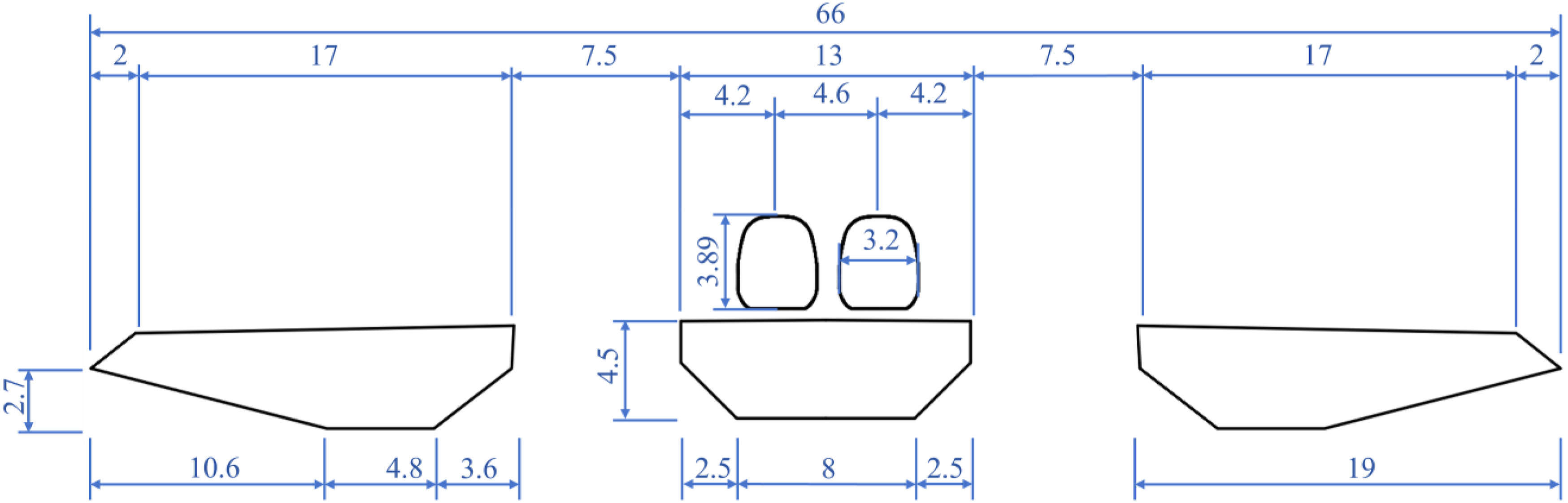

This study primarily examines the VIV response under different train-placement cases with trains arranged on the railway box girder; the considered simulation cases are listed in Figure 2. Specifically, Case 1 denotes a single train located on the windward-side railway track, Case 2 denotes a single train located on the leeward-side railway track, and Case 3 denotes the two-train case, in which trains are simultaneously arranged on both the windward-side and leeward-side railway tracks. The inflow wind speed in the 1:60 scaled-model ranges from 1 to 2 m/s. In the present study, the wind attack angle is fixed at 0°, with the incoming flow perpendicular to the bridge axis. In the numerical simulations, the train–bridge system is simplified as a vertically coupled single-degree-of-freedom (SDOF) system (Xiang et al., 2024). The contribution of the train mass to the total system mass and natural frequency is also taken into account by equivalently applying the train mass as a uniformly distributed load on the bridge deck. For computational simplicity, the influence of the train’s own stiffness and damping on the dynamic characteristics of the system is not considered in the 2D VIV simulations at this stage (Hankari et al., 2023).

Figure 2.

Definition of train-placement cases.

2.2. Numerical solution method

In this study, the two-dimensional section of the separated triple-box girder with trains is treated as a rigid body, and the surrounding flow is assumed to be incompressible and turbulent. To obtain the aerodynamic forces and flow-field characteristics of the train–bridge system, the unsteady Reynolds-averaged Navier–Stokes (RANS) equations are solved (Hami, 2021). The Reynolds-stress term is closed using the shear-stress transport (SST) k–ω turbulence model, which has been widely applied in numerical analyses of bridge aerodynamics and VIV of bluff bodies (Li et al., 2025a, 2025b).

The numerical simulations are performed in FLUENT using a pressure-based transient solver. The pressure–velocity coupling is achieved using the SIMPLEC algorithm. A second-order upwind scheme is used for spatial discretization, and a first-order implicit scheme is used for temporal discretization.

2.3. Computational domain and boundary conditions

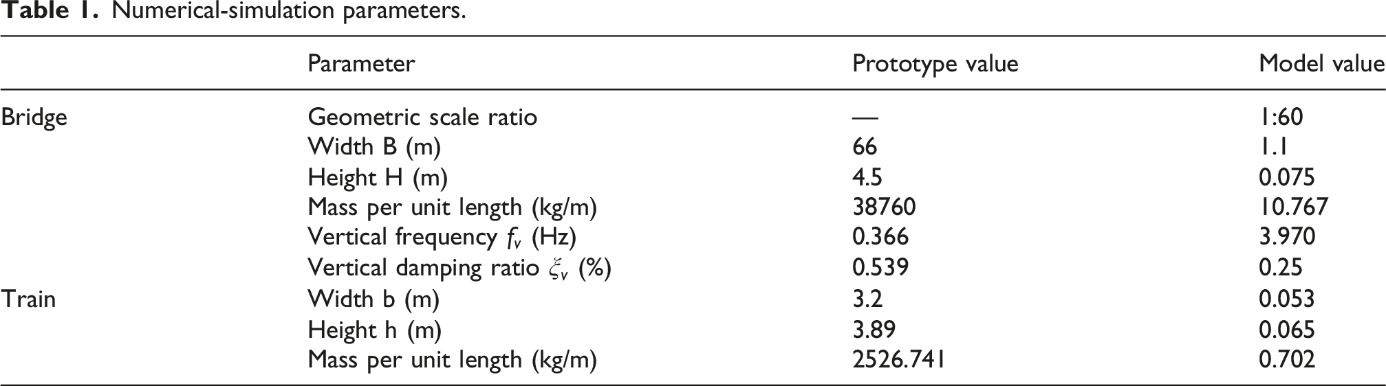
The key prototype and scaled-model parameters adopted in the numerical simulations are summarized in Table 1. A geometric scale ratio of 1:60 is used, and the sectional-model width is denoted by B for subsequent domain-size descriptions; the remaining geometric and dynamic parameters of the bridge and the train follow Table 1.

Table 1.

Numerical-simulation parameters.

	Parameter	Prototype value	Model value
Bridge	Geometric scale ratio	—	1:60
	Width B (m)	66	1.1
	Height H (m)	4.5	0.075
	Mass per unit length (kg/m)	38760	10.767
	Vertical frequency $f_{v}$ (Hz)	0.366	3.970
	Vertical damping ratio $ξ_{v}$ (%)	0.539	0.25
Train	Width b (m)	3.2	0.053
	Height h (m)	3.89	0.065
	Mass per unit length (kg/m)	2526.741	0.702

The computational domain and boundary conditions for the deck segment are shown in Figure 3. The domain width and height are 27B and 10B, respectively. The left boundary is defined as a velocity inlet, while the right boundary is defined as a pressure outlet. The top and bottom boundaries are modeled as symmetry boundaries, and the section surface is treated as a no-slip wall. The region around the section is divided into three parts: a rigid-body zone, a deforming zone, and a stationary zone. The rigid-body zone, with a size of 2B × B, is discretized using a quadrilateral mesh and moves rigidly with the triple-box girder; the outer deforming zone adopts an unstructured triangular mesh and is updated with the main-girder motion through spring-based smoothing and mesh reconstruction; the stationary zone is discretized using a quadrilateral mesh with relatively larger element sizes. The total number of mesh elements is approximately 3.2 × 10⁵. The first-layer mesh thickness on the main-girder section is 0.02 mm, satisfying y⁺ < 1 and the blockage-ratio requirement (Briggs et al., 1996).

Figure 3.

Computational model: (a) Computational domain and boundary conditions for different train-placement cases. (b) Mesh details for different train-placement cases.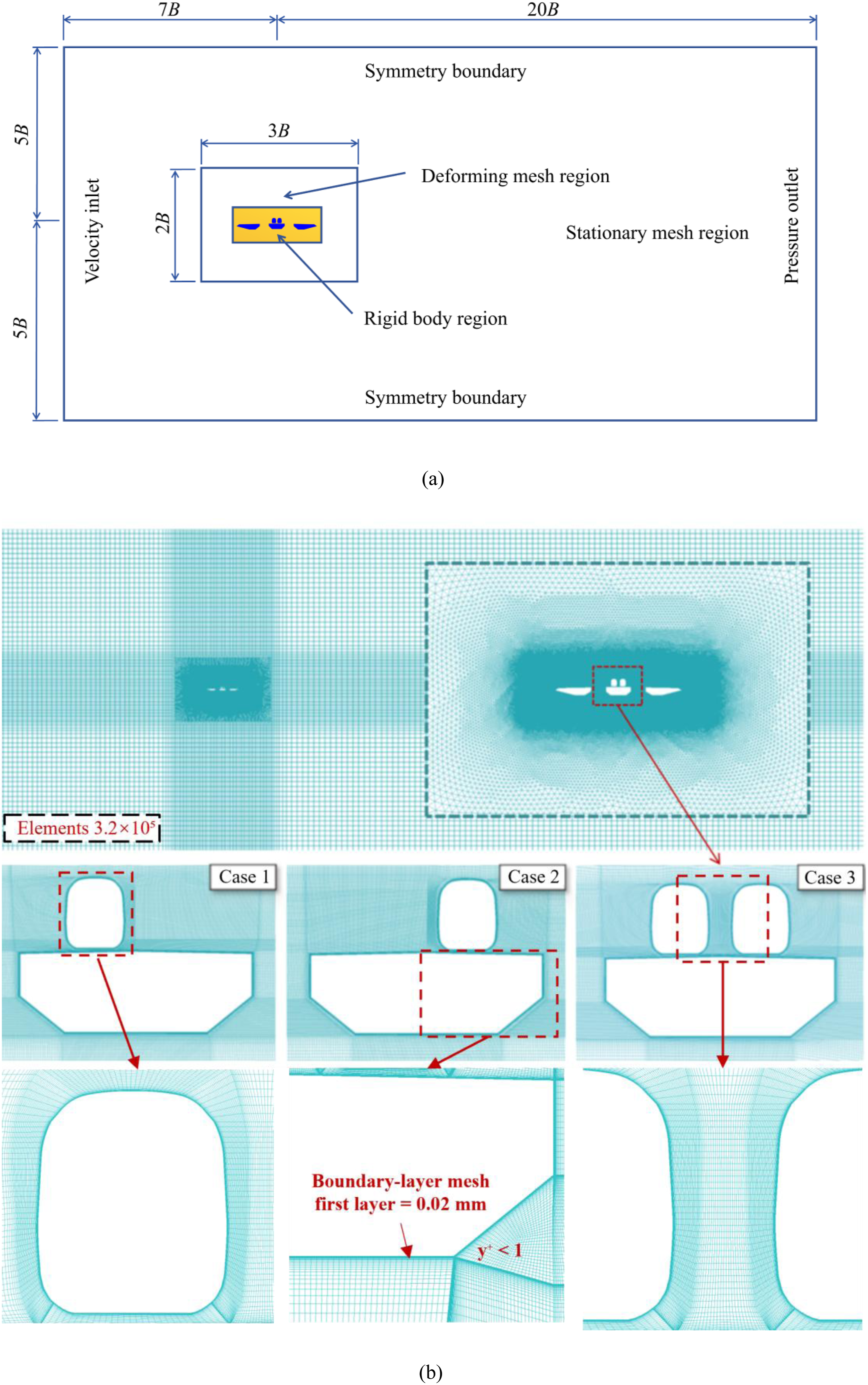

2.4. Mesh and time-step independence tests

To ensure that the numerical results are not significantly affected by the mesh resolution and time-step size, mesh and time-step independence tests were carried out before the subsequent VIV simulations. The two-train case at U/f_vB = 0.353 was selected as the representative condition, because this condition produces a relatively large vertical VIV response among the considered train-placement cases. The peak model-scale vertical VIV amplitude A_M was selected as the main comparison index.

The relative error was calculated with respect to the finest reference case, as follows: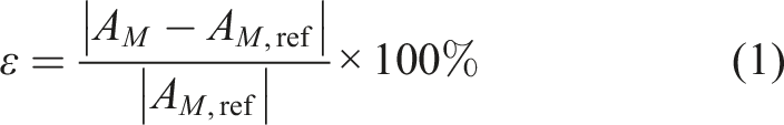

ε = \frac{| A_{M} - A_{M, ref} |}{| A_{M, ref} |} \times 100 %

(1)

where A_M is the peak model-scale vertical VIV amplitude obtained from a given mesh or time-step scheme, and A_M,ref is the corresponding value obtained from the finest reference scheme.

For the mesh-independence test, four mesh schemes with 1.4 × 10⁵, 2.1 × 10⁵, 3.2 × 10⁵, and 4.8 × 10⁵ elements were examined. The mesh with 4.8 × 10⁵ elements was taken as the reference mesh. As shown in Figure 4(a), the calculated peak amplitude increases with mesh refinement, while the relative error decreases markedly. When the number of mesh elements increases from 2.1 × 10⁵ to 3.2 × 10⁵, the relative error decreases from 4.97% to 0.94%. Further refinement to 4.8 × 10⁵ elements produces only a slight change in the peak amplitude. Therefore, considering both numerical accuracy and computational cost, the mesh scheme with 3.2 × 10⁵ elements was adopted in the subsequent simulations.

Figure 4.

Mesh and time-step independence tests: (a) mesh-independence test; (b) time-step-independence test.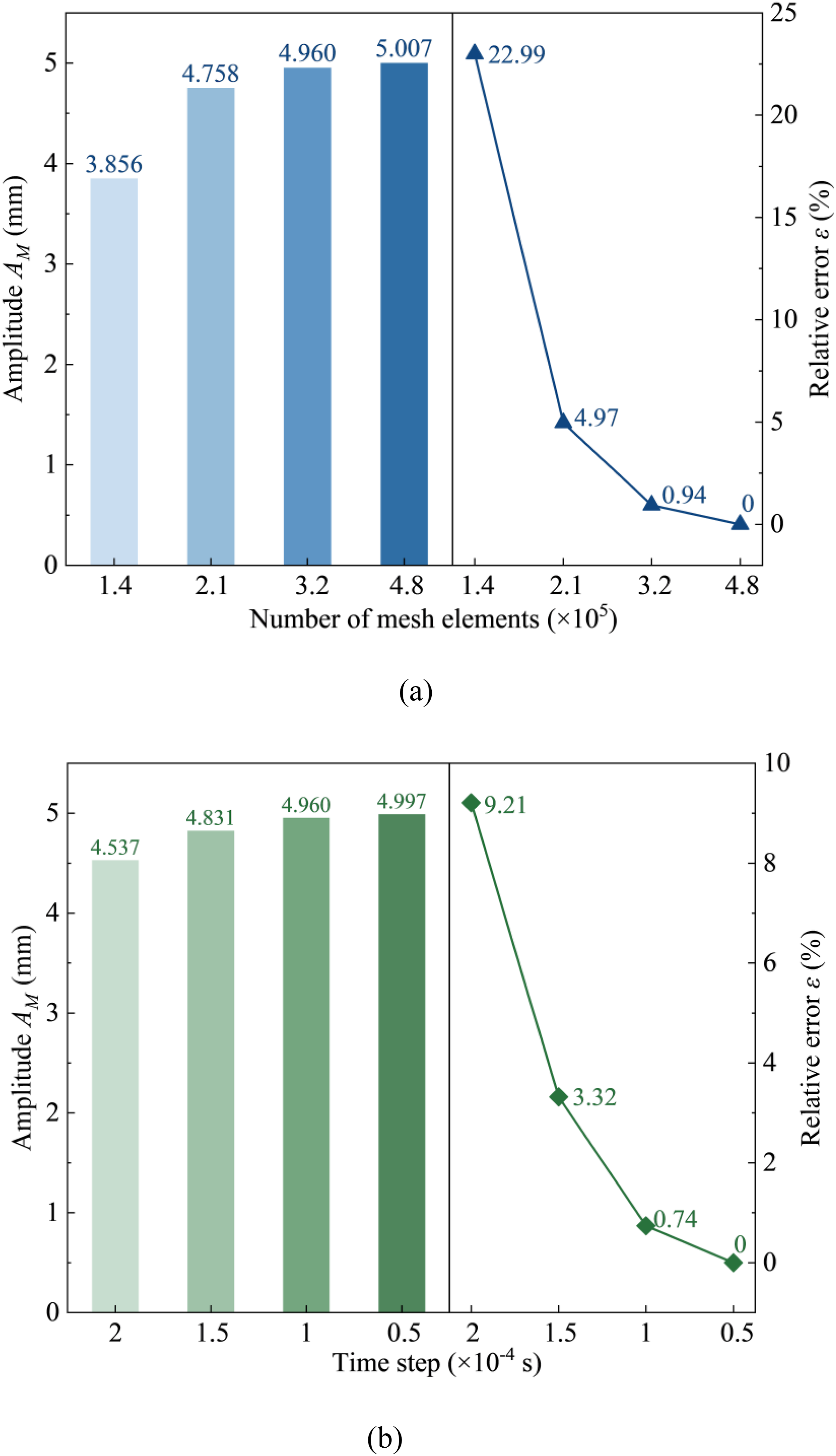

For the time-step-independence test, four time-step sizes, Δt = 2.0 × 10⁻⁴, 1.5 × 10⁻⁴, 1.0 × 10⁻⁴, and 5.0 × 10⁻⁵ s, were examined based on the selected mesh scheme. The result obtained with Δt = 5.0 × 10⁻⁵ s was used as the reference solution. As shown in Figure 4(b), the relative error decreases from 9.21% to 0.74% when Δt is reduced from 2.0 × 10⁻⁴ to 1.0 × 10⁻⁴ s. Further reducing Δt to 5.0 × 10⁻⁵ s leads to only a limited change in the calculated peak amplitude. Therefore, Δt = 1.0 × 10⁻⁴ s was adopted for the subsequent unsteady VIV simulations. These results indicate that the selected mesh resolution and time-step size are sufficient to capture the main VIV response of the train–bridge system.

2.5. Model validation

The numerical model for the bare separated triple-box girder adopts the numerical settings of Li et al. (2026) and has been validated against wind tunnel results (Wang et al., 2022), as shown in Figure 5(a). A simplified CRH3 train model following Li and He (2020) is then introduced to simulate train–bridge aerodynamic interference. In addition, the static aerodynamic coefficients of the train–bridge system at a wind attack angle of 0° are further validated against the wind tunnel results reported by Yang et al. (2022a), as shown in Figure 5(b). The purpose of this comparison is to examine whether the adopted numerical model can reasonably capture the aerodynamic-force levels of both the train and the main girder. Since the subsequent VIV analysis and the reconstruction of train aerodynamic-force fluctuation time histories require reliable aerodynamic-force inputs, this validation provides a basis for the following analyses. Overall, the comparison results show that the present model can reasonably reproduce the aerodynamic characteristics of the train–bridge system.

Figure 5.

Validation of the aerodynamic numerical model: (a) validation of the bare-girder sectional model (Li et al., 2026); (b) comparison of the static aerodynamic coefficients of the train and main girder.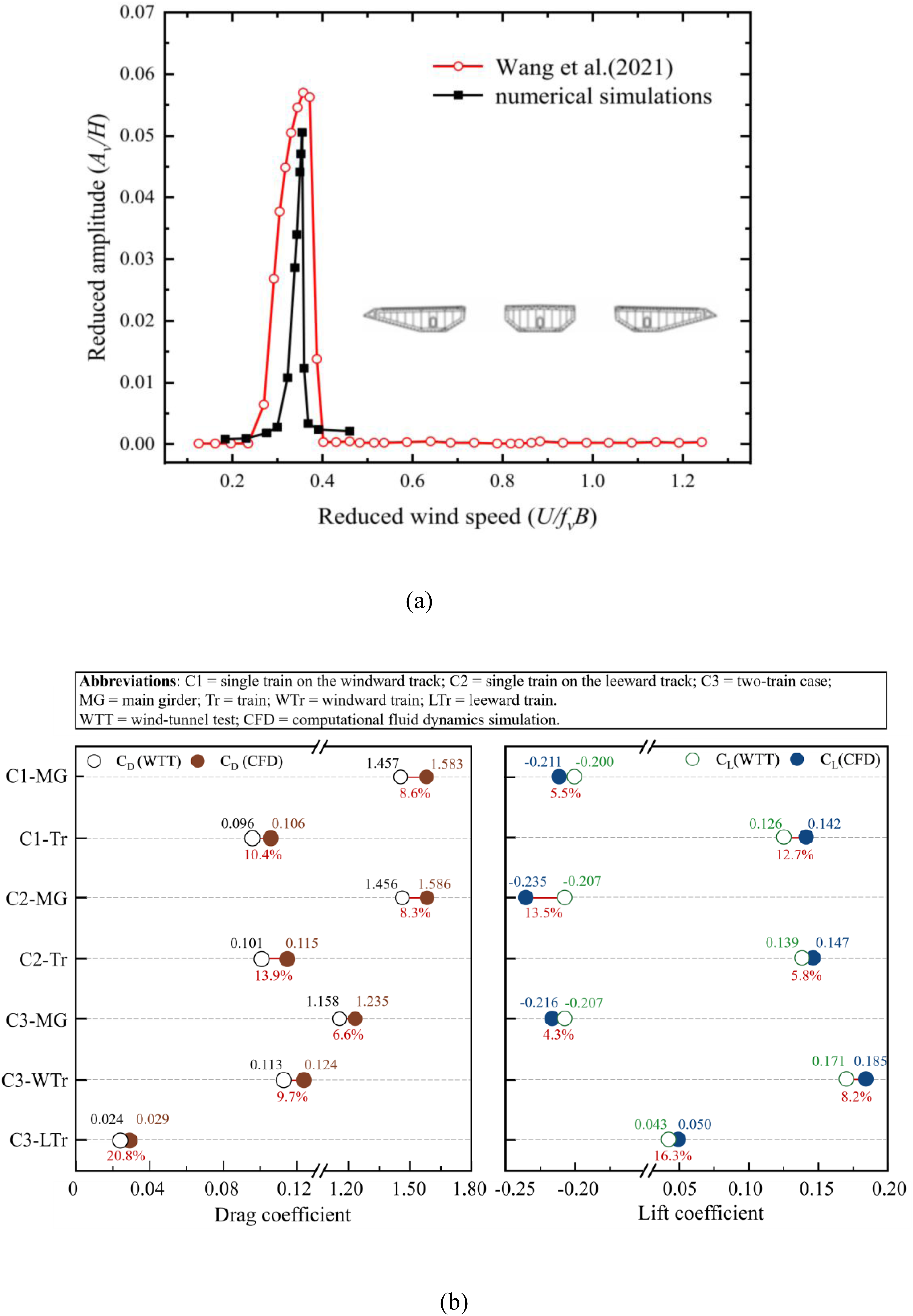

3. Analysis of aerodynamic characteristics and flow-field features

3.1. Simulation of vibration characteristics

Using an FSI approach, the vertical VIV performance of the separated triple-box girder under different train-placement cases was simulated at a wind attack angle of 0°. Figure 6 shows the reduced vertical VIV amplitude A_v/H versus the reduced wind speed U/f_vB, where U is the mean wind speed, f_v is the first-order vertical natural frequency, B is the deck width, A_v is the peak vertical displacement amplitude, and H is the girder depth.

Figure 6.

Numerical-simulation results of VIV under different train-placement cases.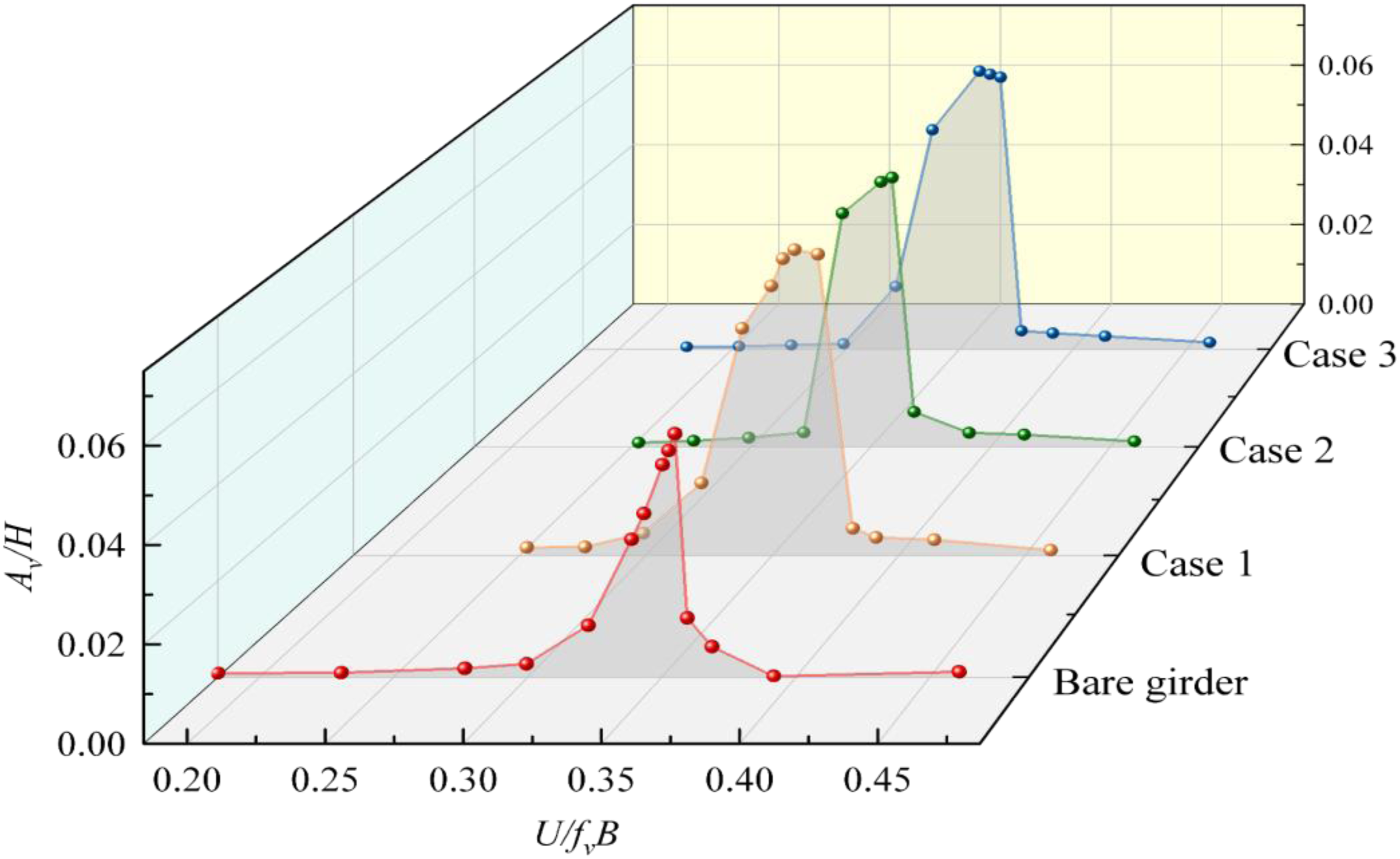

The results indicate that the presence of trains reconstructs the flow field around the bridge, thereby widening the VIV lock-in range and increasing the vibration amplitude. The peak responses of all cases occur near U/f_vB = 0.353. Taking the peak value of the bare-girder case (approximately 0.050) as the reference, the peak amplitudes in the single-train windward case, single-train leeward case, and two-train case increase by 34.6%, 25.2%, and 36.2%, respectively. Among them, the two-train case is the most unfavorable scenario. It is noteworthy that the response level of the single-train windward case is very close to that of the two-train case, which preliminarily suggests that the windward-track train plays a dominant role in governing the VIV response.

3.2. Train aerodynamic loads under VIV

For a more detailed analysis of train–bridge aerodynamic interference, the most unfavorable reduced wind speed, U/f_vB = 0.353, is selected. Figure 7 compares the lift and drag coefficients of the train under different train-placement cases, together with their time-averaged values. The time-averaged values shown in the figure are calculated using the data after 18 s, when the mean coefficients have reached temporal convergence. As shown in Figure 7(a), the lift coefficient exhibits clear differences under different train-placement cases. The mean lift coefficients in Cases 1 and 2 are 0.160 and 0.152, respectively, which are relatively close. In Case 3, a pronounced asymmetry is observed between the lift responses of the windward-track train and the leeward-track train. The lift coefficient of the windward-track train remains mostly positive, with a mean value of 0.217, whereas the mean lift coefficient of the leeward-track train is only 0.041, with more intense fluctuations and frequent switches between positive and negative values.

Figure 7.

Time histories and mean values of train aerodynamic-force coefficients under different train-placement cases (U/f_vB = 0.353): (a) train lift coefficient; (b) train drag coefficient.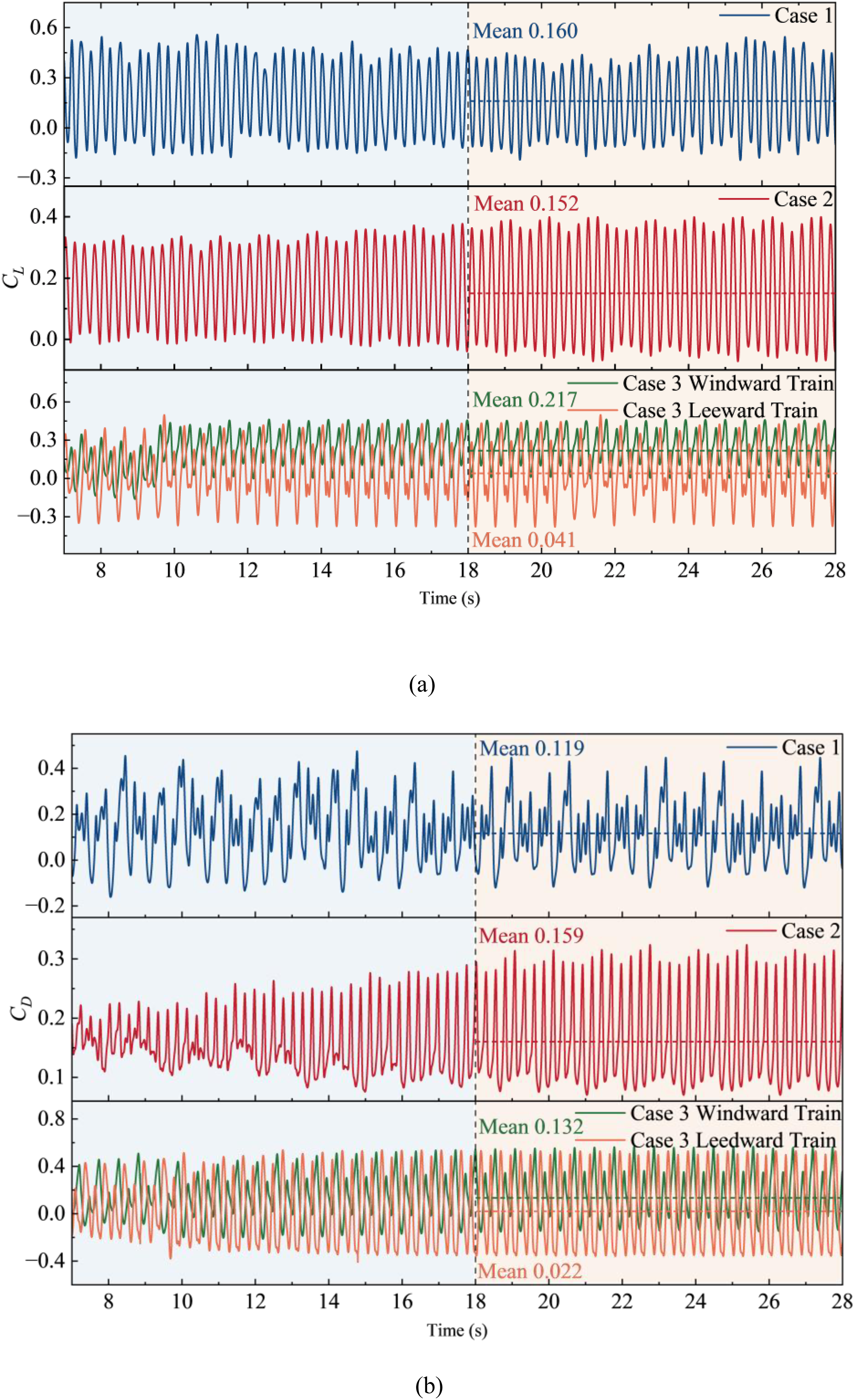

As shown in Figure 7(b), the drag coefficient in Case 3 also exhibits a similar asymmetric characteristic. The mean drag coefficient of the windward-track train is 0.132, whereas that of the leeward-track train is only 0.022, and the corresponding time history fluctuates around a value close to zero. This indicates that the leeward-track train is subjected to a pronounced shielding effect from the wake of the windward-track train. Overall, train placement significantly affects both the mean level and fluctuation intensity of the aerodynamic loads acting on the train, and may further influence the running safety and ride comfort of on-bridge trains.

3.3. Flow-field visualization

To further clarify the influence of train placement on vortex-shedding evolution and the VIV response of the main girder at different reduced wind speeds, Figure 8 compares the vorticity evolution of the bare-girder case and the train-involved Cases 1–3 at four instants within one shedding cycle for three representative reduced wind speeds, U/f_vB = 0.336, 0.353, and 0.389. The presence of trains introduces an additional separated shear layer near the train roof, which interacts with the shear layer over the upper surface of the main girder, thereby altering the wake-shedding process and its stability.

Figure 8.

Vorticity evolution contours of the separated triple-box girder under different cases and reduced wind speeds.

At U/f_vB = 0.336, the bare girder exhibits a relatively regular shedding pattern, whereas the second gap vortex in Case 2 is strengthened, indicating reduced wake stability. At U/f_vB = 0.353, Cases 1 and 3 show more concentrated upper vortex packets and more evident merging; by contrast, in Case 2, the upper and lower vortical structures are transported nearly in parallel, and the alternating shedding is weakened. The similar vortex evolution in Cases 1 and 3 also corresponds to their comparable VIV amplitudes, indicating that the windward-track train has a pronounced influence on the flow field and vertical VIV response at this reduced wind speed. At U/f_vB = 0.389, the wake unsteadiness of the bare girder is further enhanced. Under this condition, Case 2 is more prone to forming larger-scale vortex packets and exhibits a more evident tendency toward alternating shedding, whereas in Case 3 the vortices above the train remain continuously connected after shedding, thereby suppressing the alternating shedding to some extent. The different wake organizations of Cases 2 and 3 at the same reduced wind speed indicate that train placement can modify the vortex-shedding pattern and contribute to the differences in VIV responses among different train-placement cases.

4. Influence of vertical VIV on train running performance

4.1. Wind–vehicle–track–bridge coupled dynamic model

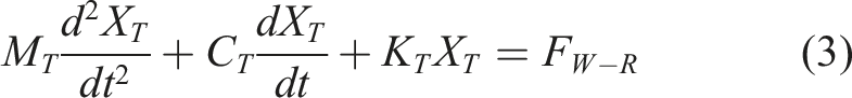
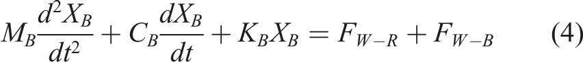
To analyze the influence of vertical VIV on the running performance of on-bridge trains, a wind–vehicle–track–bridge coupled dynamic model is established, consisting of the vehicle subsystem, track subsystem, and bridge subsystem. The vehicle subsystem is represented by a multi-rigid-body model, the track subsystem by a discretely supported track model, and the bridge subsystem by a finite-element model. Dynamic coupling among the subsystems is achieved through the wheel–rail interaction and the track–bridge interaction. The bridge VIV-induced displacement excitation and the train aerodynamic load inputs are incorporated into the coupled time-domain analysis, as detailed in Sections 4.2 and 4.3.

The vertical VIV is introduced in the form of an equivalent track-irregularity excitation, while the train aerodynamic excitation is incorporated through the reconstructed aerodynamic-force fluctuation time histories of the train under VIV, as shown in Figure 9. Based on the above assumptions, the equations of motion of the vehicle subsystem, track subsystem, and bridge subsystem can be written as:

Figure 9.

Procedure for introducing vertical VIV into the wind–vehicle–track–bridge coupled dynamic analysis.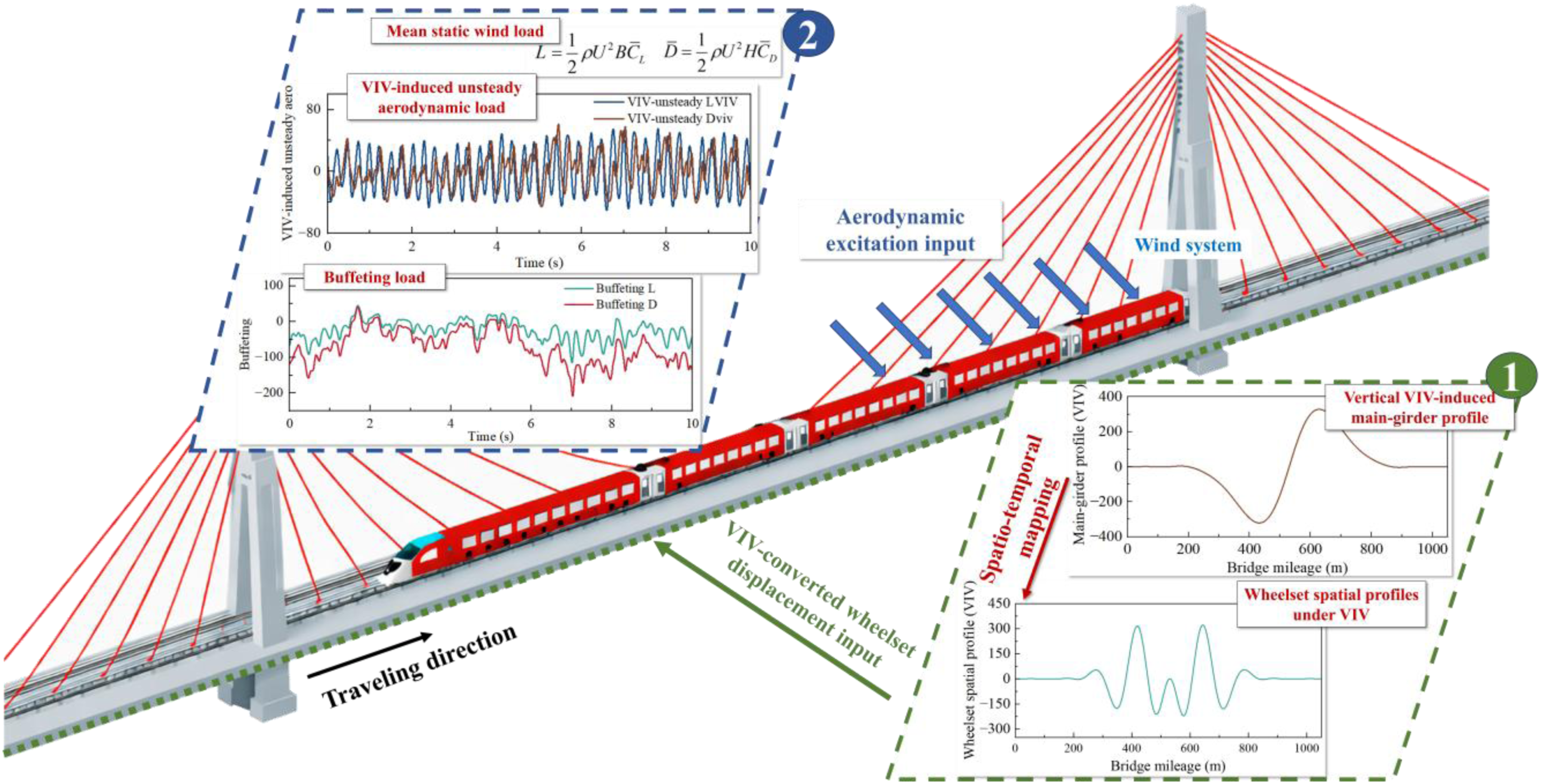

In the present model, the reconstructed bridge VIV displacement is superimposed with the original track irregularity along the train running path and then introduced into the wheel–rail relative displacement relationship (Liu et al., 2023; Luo et al., 2022). The resulting wheel–rail interaction force acts simultaneously on the vehicle and track subsystems, and is further transmitted to the bridge subsystem through the track–bridge interaction.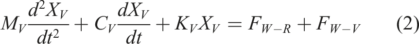

M_{V} \frac{d^{2} X_{V}}{d t^{2}} + C_{V} \frac{d X_{V}}{d t} + K_{V} X_{V} = F_{W - R} + F_{W - V}

(2)

M_{T} \frac{d^{2} X_{T}}{d t^{2}} + C_{T} \frac{d X_{T}}{d t} + K_{T} X_{T} = F_{W - R}

(3)

M_{B} \frac{d^{2} X_{B}}{d t^{2}} + C_{B} \frac{d X_{B}}{d t} + K_{B} X_{B} = F_{W - R} + F_{W - B}

(4)

where

\frac{d^{2} X_{V}}{d t^{2}}

\frac{d X_{V}}{d t}

, and

X_{V}

denote the acceleration, velocity, and displacement vectors of the vehicle subsystem, respectively;

\frac{d^{2} X_{T}}{d t^{2}}

\frac{d X_{T}}{d t}

, and

X_{T}

denote those of the track subsystem; and

\frac{d^{2} X_{B}}{d t^{2}}

\frac{d X_{B}}{d t}

, and

X_{B}

denote those of the bridge subsystem. Similarly, M, C, and K represent the mass, damping, and stiffness matrices, respectively, with the subscripts V, T, and B indicating the vehicle, track, and bridge subsystems. In addition,

F_{W - R}

denotes the wheel–rail interaction force, whereas

F_{W - V}

and

F_{W - B}

represent the aerodynamic loads acting on the vehicle and bridge, respectively.

4.2. Construction and equivalent mapping of vertical VIV displacement excitation

The VIV amplitudes obtained from the 2D CFD simulations are converted into the three-dimensional (3D) deformation of the full-scale bridge to evaluate the influence of VIV on the running performance of on-bridge trains. Such sectional-to-full-bridge linkage has been widely used in VIV studies (Wang et al., 2025; Zhang, 2023), and 2D sectional CFD has also been employed as a numerical counterpart for identifying and predicting sectional VIV responses (Noguchi et al., 2020; Wang and Chen, 2022).

This conversion is based on the following assumptions. The sectional VIV amplitude obtained from the 2D CFD simulation is taken as the representative response of the mid-span section. The full-bridge vertical VIV deformation is assumed to be mainly governed by the target vertical mode, and its spanwise distribution is described by the corresponding mode-shape function. The reconstructed full-bridge deformation is then introduced into the wind–vehicle–track–bridge coupled dynamic model as an equivalent wheelset displacement excitation.

Following the amplitude-conversion approach proposed by Zhang and Chen (2011), the sectional vertical amplitude A_M is converted into the corresponding prototype mid-span amplitude A_p, and the conversion formula is given as follows: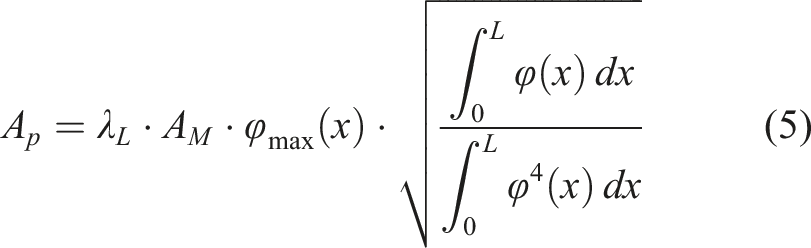

A_{p} = λ_{L} \cdot A_{M} \cdot φ_{\max} (x) \cdot \sqrt{\frac{\int_{0}^{L} φ (x) d x}{\int_{0}^{L} φ^{4} (x) d x}}

(5)

where

λ_{L}

is the geometric scale ratio, taken as 1:60;

φ (x)

is the first-order vertical mode-shape function of the prototype bridge, whose specific form is determined from the finite-element modal analysis of the bridge; and

φ_{\max}

is its maximum value.

It should be noted that this sectional-to-full-bridge mapping is not intended to reproduce the complete three-dimensional aeroelastic response of the full bridge, but is adopted as a displacement-based equivalent-excitation treatment. The reconstructed full-bridge displacement is introduced into the wind–vehicle–track–bridge coupled dynamic model as the bridge VIV-induced vertical input. Since the displacement field is constructed based on the target vertical mode shape and the converted mid-span amplitude, it can reasonably represent the dominant vertical VIV deformation required for the running-performance analysis.

Based on the above formula, the VIV response at the most unfavorable reduced wind speed U/f_vB = 0.353 is selected, and the 2D amplitudes for each case are converted into the corresponding prototype vertical amplitudes, as summarized in Table 2.

Table 2.

Conversion results from 2D sectional VIV amplitude to prototype bridge vertical VIV response (U/f_vB = 0.353).

Case	2D amplitude (mm)	Prototype amplitude (mm)
Case 1 (single train on the windward-side railway track)	4.873	328.471
Case 2 (single train on the leeward-side railway track)	4.699	316.742
Case 3 (the two-train case)	4.960	334.335

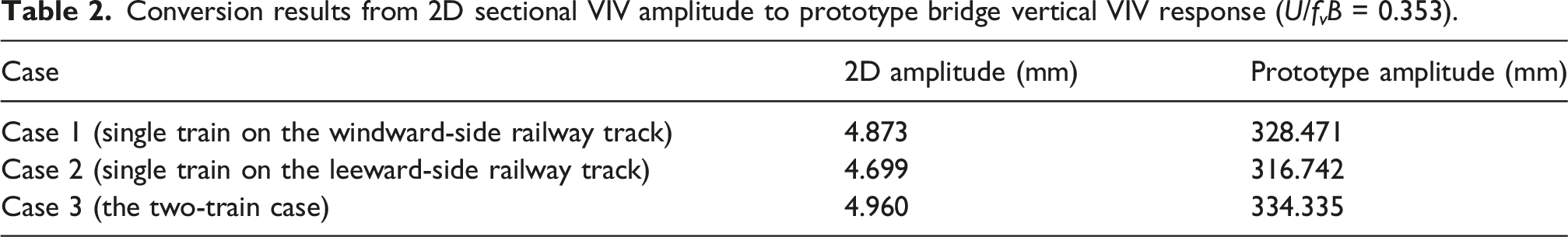
On this basis, to further evaluate the effect of vertical VIV on train running performance, the VIV deformation of the prototype bridge must be converted into dynamic excitations during train passage. Similar equivalent-excitation treatments have been adopted in train–bridge coupled dynamic analyses, where bridge deformation or vibration is introduced as additional track or wheelset excitation to evaluate vehicle dynamic responses (Li et al., 2022; Wang et al., 2023a). The spatial deformation of the bridge under vertical VIV is determined based on the prototype VIV amplitude and the corresponding mode-shape distribution. The original vertical track irregularities used in the coupled dynamic analysis are generated based on the German low-disturbance spectrum and expressed as spatial-domain profiles along the train running path. The VIV-induced wheelset spatial profiles are obtained along the train running path and then superimposed with the original track irregularities in the spatial domain. Then, according to the instantaneous wheelset positions as the train traverses the bridge, the combined spatial excitation is converted into the corresponding time-domain inputs for the subsequent running-performance analysis. At a train speed of 200 km/h, the wheelset spatial profiles obtained for the three cases are illustrated in Figure 10.

Figure 10.

Wheelset spatial profiles under different cases at a train speed of 200 km/h.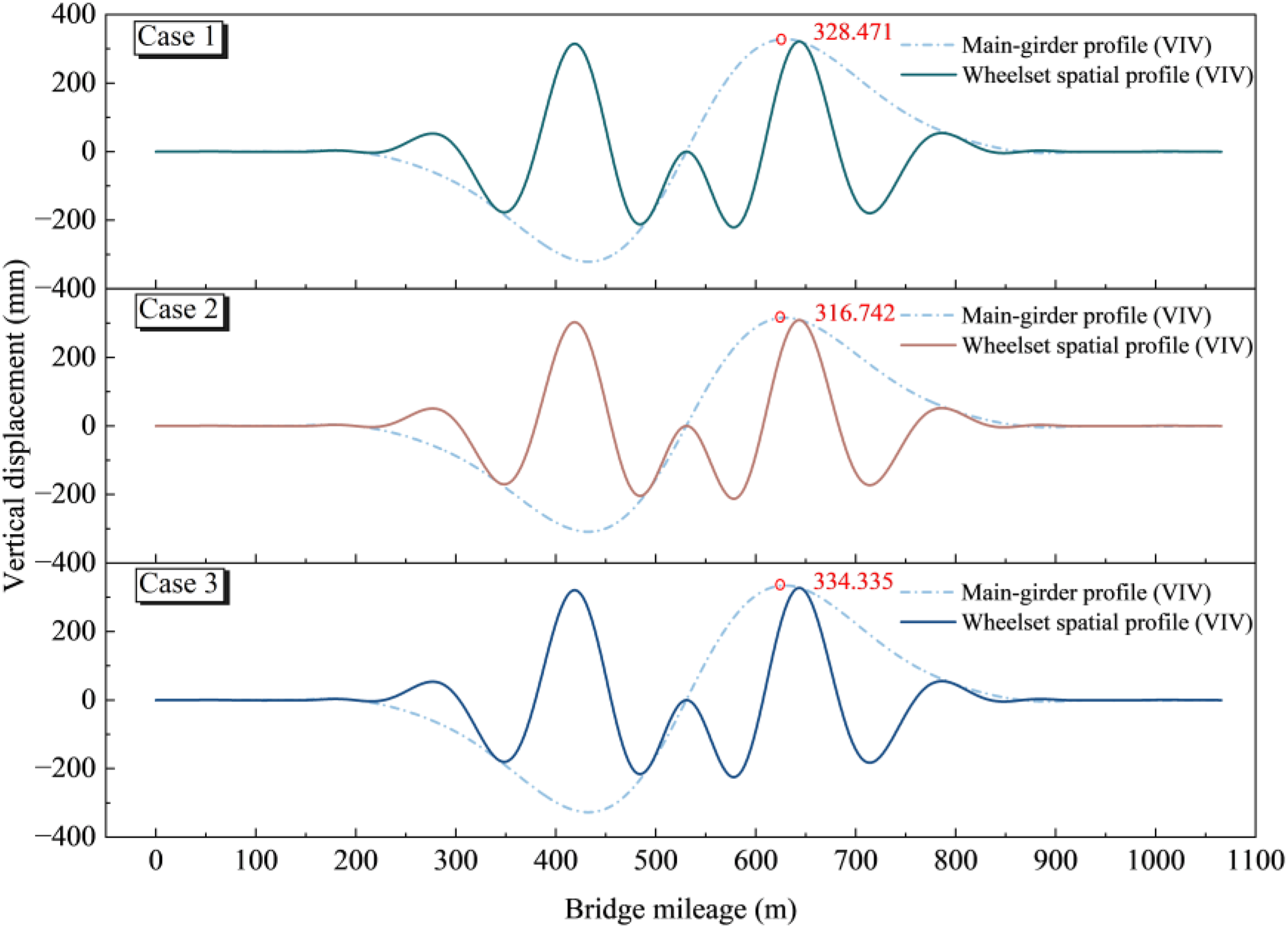

4.3. Construction and implementation of aerodynamic inputs

To ensure consistent aerodynamic inputs for the subsequent time-domain wind–vehicle–track–bridge coupled analysis, the aerodynamic loads acting on the train and the bridge are expressed in the time domain. As shown in equations (6) and (7), the total aerodynamic loads on the train are decomposed into a mean static component, a VIV-induced unsteady component, and a buffeting component. For consistency with the coupled-analysis framework, the VIV-induced unsteady and buffeting components are hereafter collectively referred to as the aerodynamic-force fluctuation time histories of the train under VIV.

L (t) = \bar{L} + L_{V I V} (t) + L_{b u} (t)

(6)

D (t) = \bar{D} + D_{V I V} (t) + D_{b u} (t)

(7)

where

L (t)

and

D (t)

denote the total lift and drag loads, respectively;

\bar{L}

and

\bar{D}

are the mean lift and drag components, respectively;

L_{V I V} (t)

and

D_{V I V} (t)

are the VIV-induced unsteady lift and drag components, respectively;

L_{b u} (t)

and

D_{b u} (t)

are the buffeting lift and drag components, respectively.

The mean static component is obtained from the time-averaged aerodynamic-coefficient time histories. To avoid double counting in load superposition, the aerodynamic coefficients extracted from the CFD/FSI simulations are de-meaned, thereby yielding the VIV-induced unsteady lift and drag time histories. The buffeting component is formulated based on Scanlan’s quasi-steady theory; the fluctuating wind-speed time histories required for the buffeting calculation are generated as follows.

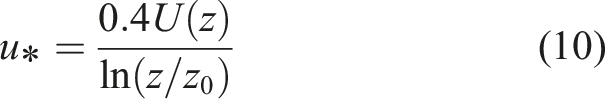
The fluctuating wind-speed time histories used for calculating the buffeting component are generated using the harmonic superposition method. The longitudinal and vertical fluctuating wind components are simulated according to the Kaimal spectrum and the Panofsky spectrum, respectively. Their one-sided power spectral density functions are expressed as equations (8)–(9).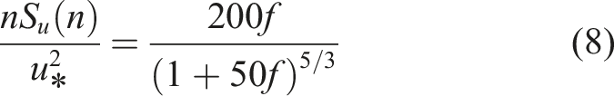

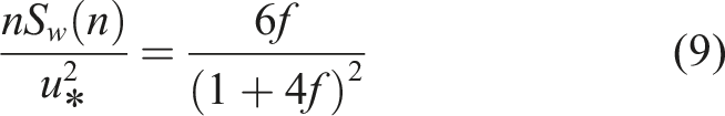
\frac{n S_{u} (n)}{u_{*}^{2}} = \frac{200 f}{{(1 + 50 f)}^{5 / 3}}

(8)

\frac{n S_{w} (n)}{u_{*}^{2}} = \frac{6 f}{{(1 + 4 f)}^{2}}

(9)

where

S_{u} (n)

and

S_{w} (n)

are the longitudinal and vertical fluctuating wind-speed spectra, respectively;

n

is the fluctuating wind frequency;

f = n z / U (z)

is the Monin coordinate;

z

is the height above the ground;

U (z)

is the mean wind speed at height

z

; and

u_{*}

is the friction velocity, calculated using equation (10).

u_{*} = \frac{0.4 U (z)}{\ln (z / z_{0})}

(10)

where

z_{0}

is the surface roughness height. In this study, z = 32 m,

U (z)

= 8.53 m/s,

z_{0}

= 0.01 m. Accordingly,

u_{*}

= 0.423 m/s is obtained from equation (10).

The spatial correlation of the fluctuating wind field is described using the Davenport coherence function, as given in equation (11).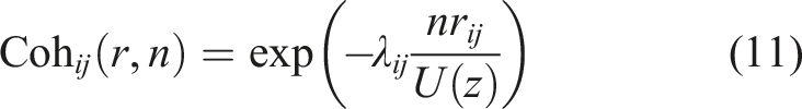

{Coh}_{i j} (r, n) = \exp (- λ_{i j} \frac{n r_{i j}}{U (z)})

(11)

where

r_{i j}

is the distance between computational points i and j, and

λ_{i j}

is the coherence decay coefficient. The fluctuating wind-speed time histories are generated at the aerodynamic loading points used in the coupled dynamic analysis. The spatial correlation between different loading points is considered using the Davenport coherence function, with

λ_{i j} = 7

. Based on the target spectra and coherence function, the harmonic superposition method is used to generate the spatially correlated fluctuating wind-speed time histories, which are then used to calculate the buffeting lift and drag time histories.

In the coupled dynamic analysis, the train subsystem is subjected to the mean static wind loads and the aerodynamic-force fluctuation time histories of the train under VIV simultaneously. On the bridge side, only the mean static wind load is considered, because the VIV-related dynamic effect within the lock-in range has already been represented by the displacement excitation introduced as an equivalent track irregularity.

4.4. Dynamic response analysis of the train under vertical VIV

To investigate the running performance of on-bridge trains under vertical VIV conditions, the bridge VIV-induced displacement excitation and train aerodynamic load inputs are incorporated into the time-domain wind–vehicle–track–bridge coupled dynamic analysis. The analysis conditions are listed in Table 3. Analysis Condition A adopts the full-bridge VIV displacement input for the bare-girder case. In contrast, Analysis Conditions B and C adopt the train-involved VIV responses obtained in the present study. The only difference between Conditions B and C lies in the train aerodynamic input. Condition B adopts the mean lift and drag coefficients of the train under VIV, whereas Condition C further considers the aerodynamic-force fluctuation time histories of the train under VIV. The results show that, after train participation is taken into account, both the carbody vertical acceleration and wheel load reduction rate increase. When the aerodynamic-force fluctuation time histories of the train under VIV are further considered, the carbody vertical acceleration changes only slightly, whereas the wheel load reduction rate becomes more sensitive.

Table 3.

Analysis conditions and corresponding inputs.

Analysis condition	Bridge VIV displacement input	Train aerodynamic load input	Description
Analysis Condition A	Converted from the bare-girder CFD amplitude reported by Li et al. (2026)	Wind tunnel test lift and drag coefficients	Without train–bridge aerodynamic interference
Analysis Condition B	Converted from the train-involved CFD amplitude in this study	Mean lift and drag coefficients under VIV	Mean aerodynamic condition considering train–bridge aerodynamic interference
Analysis Condition C	Converted from the train-involved CFD amplitude in this study	Fluctuation time histories of lift and drag coefficients under VIV	Aerodynamic-force fluctuation condition considering train–bridge aerodynamic interference

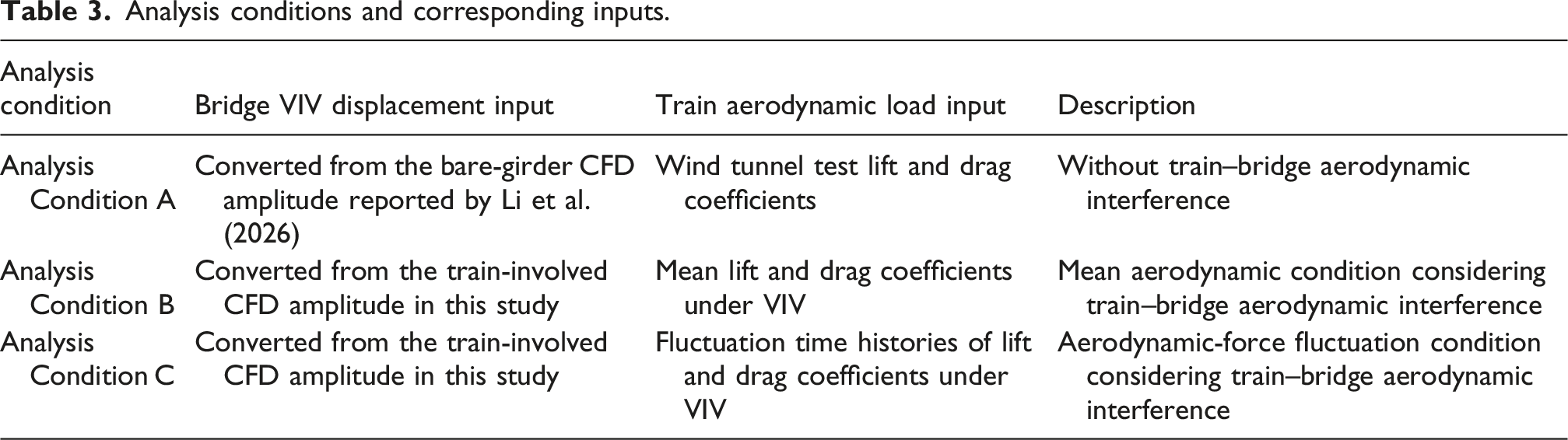
Figure 11 presents the carbody vertical acceleration responses of trains running at 200 km/h under different analysis conditions. Under different analysis conditions, the main oscillation regions of the carbody vertical acceleration are generally consistent. The response peaks are mainly concentrated in the bridge segment with significant vertical VIV response. This indicates that the carbody vertical response is mainly governed by the bridge vertical vibration under VIV. Under Analysis Condition A, the time-history patterns of different train-placement cases are generally similar, with only slight differences in the peak values. Among them, Case 1 shows the largest peak value of 1.218 m/s². Under Analysis Condition B, the overall time-history pattern of the carbody vertical acceleration changes only slightly, whereas the peak values increase in all cases. In particular, for the windward-track train in Case 3, the peak value increases from 1.132 m/s² to 1.282 m/s², corresponding to an increase of 13.25%.

Figure 11.

Carbody vertical acceleration responses of trains running at 200 km/h under different analysis conditions: (a) comparison between Analysis Conditions A and B; (b) comparison between Analysis Conditions A and C.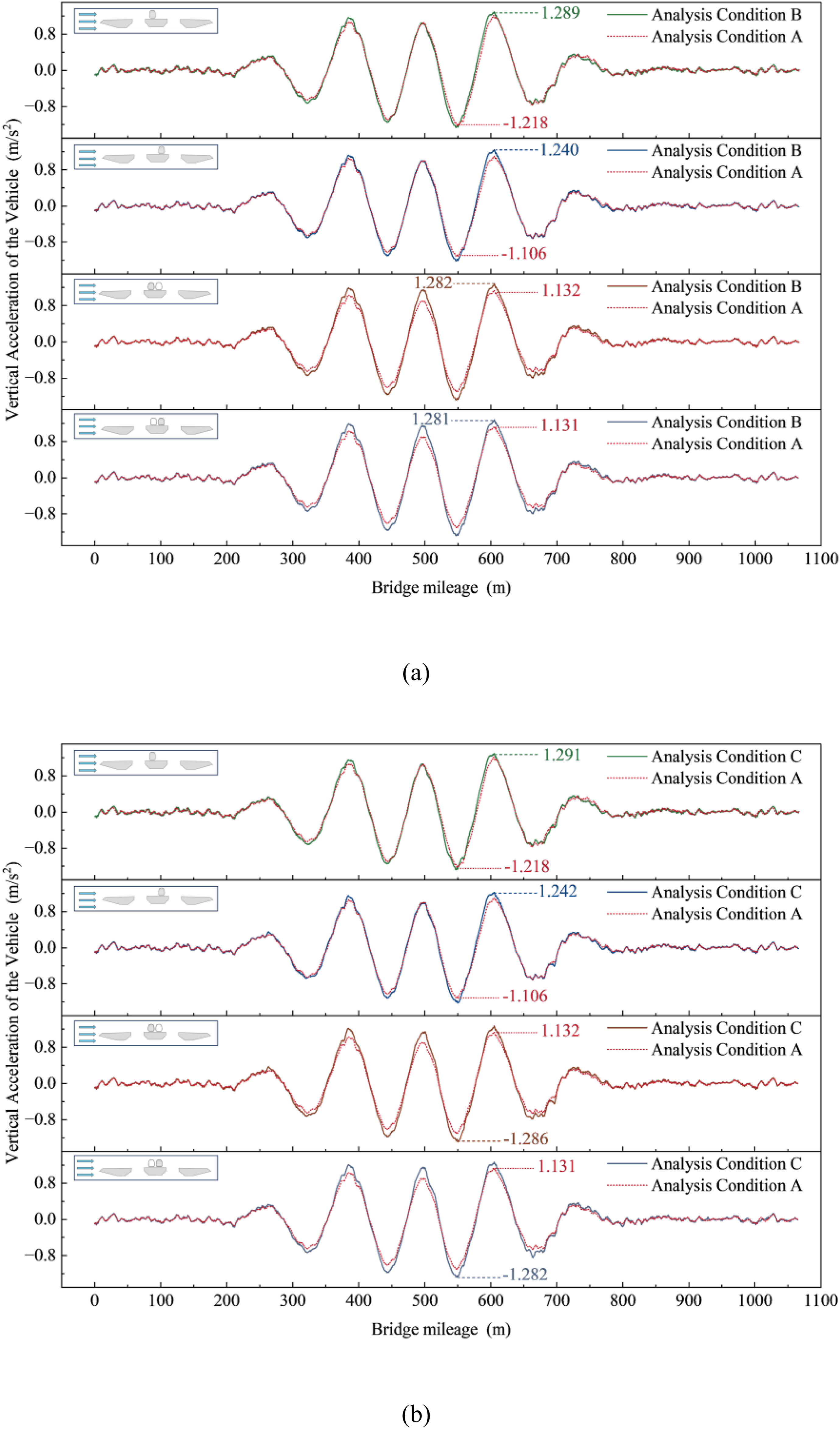

Under Analysis Condition C, the carbody vertical acceleration changes only slightly when the aerodynamic-force fluctuation time histories of the train under VIV are further considered. This indicates that the influence of such fluctuating aerodynamic loads on this response is limited. This is because the bridge VIV-induced displacement input is dominated by low-frequency components, whereas the higher-frequency components contained in the aerodynamic-force fluctuations are effectively attenuated by the suspension system. In addition, train placement has a limited influence on this response. In the two-train case, the carbody vertical acceleration of the leeward-track train decreases slightly due to the shielding effect of the windward-track train. This is generally consistent with the results of the preceding two-dimensional flow-field analysis.

Before analyzing the wheel load reduction rate, its definition is given based on the vertical wheel–rail contact force obtained from the coupled dynamic model. For the $i$ -th wheel, the time-varying wheel load reduction rate is calculated as

η_{i} (t) = \frac{Q_{0, i} - Q_{i} (t)}{Q_{0, i}}

(12)

where

η_{i} (t)

is the wheel load reduction rate of the i-th wheel,

Q_{0, i}

is the static wheel load, and

Q_{i} (t)

is the instantaneous vertical wheel–rail contact force directly obtained from the wheel–rail interaction in the coupled dynamic model. In this study, the wheel load reduction rate time history of each train is obtained by taking the maximum

η_{i} (t)

among all wheels at each time step.

Figure 12 presents the wheel load reduction rate responses of trains running at 200 km/h under different analysis conditions. Under Analysis Condition A, the response time histories of different train-placement cases are generally similar, although the peak values show certain differences. Among them, the windward-track train in Case 3 shows the largest peak value, reaching 0.294. Under Analysis Condition B, the wheel load reduction rate increases markedly in all cases, and the fluctuation amplitude is also significantly enhanced. In particular, for the windward-track train in Case 3, the peak value increases from 0.294 to 0.435, corresponding to an increase of approximately 47.96%. This indicates that, after train participation is taken into account, the modified VIV displacement input and aerodynamic loading further increase the wheel load reduction rate.

Figure 12.

Wheel load reduction rate responses of trains running at 200 km/h under different analysis conditions: (a) comparison between Analysis Conditions A and B; (b) comparison between Analysis Conditions A and C.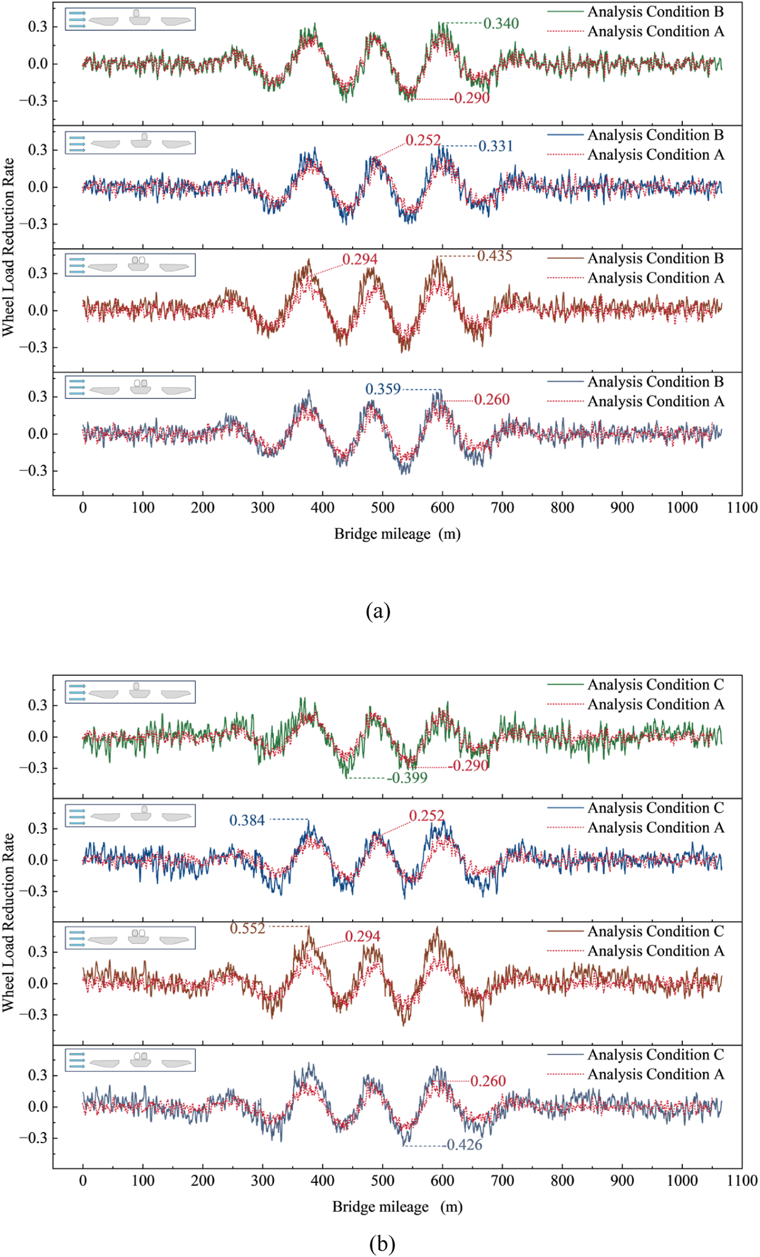

Under Analysis Condition C, the stochastic fluctuations of the wheel load reduction rate are markedly intensified when the aerodynamic-force fluctuation time histories of the train under VIV are further considered. The peak values also increase in some cases. For example, in the two-train case, the peak value of the windward-track train increases from 0.435 to 0.552, corresponding to an increase of approximately 26.90%. This indicates that the wheel load reduction rate is more sensitive to higher-frequency aerodynamic fluctuations. In the single-train case, both the fluctuation intensity and the peak value of the leeward-track train are smaller than those of the windward-track train. In the two-train case, the peak value of the windward-track train reaches 0.552, whereas that of the leeward-track train is 0.426, corresponding to a reduction of approximately 22.83% relative to the windward-track train. This indicates that the shielding effect has a more pronounced influence on the wheel load reduction rate than on the carbody vertical acceleration.

5. Conclusions

Through numerical simulations, this study investigates the VIV responses, aerodynamic characteristics, and flow-field structures of a separated triple-box girder under different train-placement cases, and further evaluates the influence of vertical VIV on the running performance of on-bridge trains. The main conclusions are as follows:

(1) The presence and placement of trains markedly affect the VIV response of the separated triple-box girder. Among the considered cases, the two-train case produces the largest vertical VIV response. The maximum reduced vertical amplitude increases by approximately 36.2% relative to the bare-girder case, and the lock-in wind-speed range is enlarged.

(2) Train–bridge aerodynamic interference makes the train aerodynamic loads sensitive to train placement, with the most pronounced aerodynamic asymmetry occurring in the two-train case. The wake of the windward-track train produces a significant shielding effect on the leeward-track train, leading to marked reductions in its lift and drag coefficients.

(3) The additional separated shear layer introduced by the train alters the evolution of the vortical structures over the upper surface of the main girder, and further affects the vortex activity within the inter-box gaps and the stability of wake shedding. For the considered train-placement cases, the single-train leeward case tends to strengthen the second gap vortex and reduce wake stability, whereas the two-train case tends to suppress the alternating shedding to some extent at higher reduced wind speeds.

(4) Under vertical VIV conditions, the train-involved VIV response increases both the carbody vertical acceleration and the wheel load reduction rate in the coupled dynamic analysis. When the aerodynamic-force fluctuation time histories of the train under VIV are further considered, the carbody vertical acceleration changes only slightly, whereas the wheel load reduction rate increases further. These results indicate that the bridge VIV-induced displacement excitation is important for the overall vehicle vertical response, while the aerodynamic-force fluctuation time histories of the train under VIV should be considered when assessing wheel unloading under VIV conditions.

Footnotes

ORCID iDs

Xiaozhen Li

Ming Wang

Author Contributions

Xiaozhen Li: Conceptualization, methodology, investigation, and funding acquisition. Weijie He: Conceptualization, methodology, software, formal analysis, and writing original draft. Yuhao Zheng and Zhichao Yang: Data curation, software, and visualization. Ming Wang: Project administration and validation.

Funding

The authors disclosed receipt of the following financial support for the research, authorship, and/or publication of this article: This study was supported by the National Natural Science Foundation of China under Grant Nos. 52278463 and U2468213.

Declaration of conflicting interests

The authors declared no potential conflicts of interest with respect to the research, authorship, and/or publication of this article.

Data Availability Statement

Data will be made available on request.*

Declaration of generative AI and AI-assisted technologies in the writing process

During the preparation of this work the authors used ChatGPT in order to improve language and readability. After using this tool/service, the authors reviewed and edited the content as needed and take full responsibility for the content of the publication.

References

Briggs

Ferziger

Koseff

, et al. (1996) Entrainment in a shear-free turbulent mixing layer. Journal of Fluid Mechanics 310: 215–241. https://doi.org/10.1017/s0022112096001784

Chen

Wang

Zhu

, et al. (2018) Numerical study on surface distributed vortex-induced force on a flat-steel-box girder. Engineering Applications of Computational Fluid Mechanics 12(1): 41–56. https://doi.org/10.1080/19942060.2017.1337593

Deng

Yang

Deng

, et al. (2020) Time-resolved aerodynamic loads on high-speed trains during running on a tunnel–bridge–tunnel infrastructure under crosswind. Engineering Applications of Computational Fluid Mechanics 14(1): 202–221. https://doi.org/10.1080/19942060.2019.1705396

Fujino

Yoshida

(2002) Wind-induced vibration and control of trans-Tokyo Bay crossing bridge. Journal of Structural Engineering 128(8): 1012–1025. https://doi.org/10.1061/(asce)0733-9445(2002)128:8(1012)

Hami

(2021) Turbulence modeling a review for different used methods. International Journal of Heat and Technology 39(1): 227–234. https://doi.org/10.18280/ijht.390125

Han

Liu

Guo

, et al. (2022) Research status and prospect of wind-vehicle-bridge coupling vibration system. Journal of Traffic and Transportation Engineering 9(3): 319–338. https://doi.org/10.1016/j.jtte.2021.05.002

Hankari

Tahiri

Dkiouak

, et al. (2023) On the vertical effect of the Non-linear behavior of track–bridge interaction in simply supported railway bridges. International Journal of Non-linear Mechanics 154: 104442. https://doi.org/10.1016/j.ijnonlinmec.2023.104442

Zuo

Zou

, et al. (2020) Experimental study on aerodynamic characteristics of a high-speed train on viaducts in turbulent crosswinds. Journal of Central South University 27(8): 2465–2478. https://doi.org/10.1007/s11771-020-4462-3

Peng

, et al. (2024) Recent developments in the wind resistance of railway bridges in China. Advances in Wind Engineering 1: 100027. https://doi.org/10.1016/j.awe.2024.100027

10.

Kubo

(2004) Prospects for the suppression of aeroedynamic vibrations of a long-span bridge using boundary-layer control. Journal of Vibration and Control 10(9): 1359–1373. https://doi.org/10.1177/1077546304042050

11.

(2020) Lateral aerodynamic interference between an interior train and a flat box bridge-deck. Experimental Thermal and Fluid Science 117: 110115. https://doi.org/10.1016/j.expthermflusci.2020.110115

12.

Xiang

Wang

, et al. (2022) A comprehensive review on coupling vibrations of train–bridge systems under external excitations. Railway Engineering Science 30(3): 383–401. https://doi.org/10.1007/s40534-022-00278-x

13.

Sun

Liu

, et al. (2025a) Effects and mechanisms of the main longitudinal beam shape on vortex-induced vibrations of Π-shaped composite girders. Structures 78: 109345. https://doi.org/10.1016/j.istruc.2025.109345

14.

Yang

Zhang

, et al. (2025b) Mitigation effect of guide vanes on the vortex-induced vibration of a long-span closed-box girder suspension bridge. Journal of Vibration and Control 31(9-10): 1574–1585. https://doi.org/10.1177/10775463241241100

15.

Zhang

Wang

(2026) Numerical investigation on vortex-induced vibration characteristics and vortex shedding mechanism of the triple-box girder. Journal of Vibration and Control 32(5-6): 1050–1064. https://doi.org/10.1177/10775463241308350

16.

Liu

Mei

, et al. (2023) Effect of vertical vortex-induced vibration of bridge on railway vehicle’s running performance. Vehicle System Dynamics 61(5): 1432–1447. https://doi.org/10.1080/00423114.2022.2084120

17.

, et al. (2025) Wind-induced vibration control of bridge girders by aerodynamic and mechanical methods: a literature review. Advances in Bridge Engineering 6(1): 35. https://doi.org/10.1186/s43251-025-00182-4

18.

Luo

Gan

, et al. (2022) The train-bridge coupled vibration analysis of a long-span prestressed concrete continuous beam bridge under creep deformation effect. Applied Sciences 12(22): 11838. https://doi.org/10.3390/app122211838

19.

Macdonald

JHG

Irwin

Fletcher

(2002) Vortex-induced vibrations of the second severn crossing cable-stayed bridge—Full-scale and wind tunnel measurements. Proceedings of the Institution of Civil Engineers: Structures and Buildings 152(2): 123–134. https://doi.org/10.1680/stbu.2002.152.2.123

20.

Noguchi

Ito

Yagi

(2020) Numerical evaluation of vortex-induced vibration amplitude of a box girder bridge using forced oscillation method. Journal of Wind Engineering and Industrial Aerodynamics 196: 104029. https://doi.org/10.1016/j.jweia.2019.104029

21.

Sato

Hirahara

Fumoto

, et al. (2002) Full aeroelastic model test of a super long-span bridge with slotted box girder. Journal of Wind Engineering and Industrial Aerodynamics 90(12): 2023–2032. https://doi.org/10.1016/s0167-6105(02)00318-5

22.

Song

Qian

Liu

, et al. (2025) Assessment of driving safety considering wind-vehicle-bridge coupling effects. Journal of Vibration and Control 31(21-22): 4556–4569. https://doi.org/10.1177/10775463251330854

23.

Tai

Zheng

Yan

, et al. (2025) The aerodynamic mechanism of the effect of gap width on the vertical vortex-induced vibration of the triple-box girders. Physics of Fluids 37(8): 085144. https://doi.org/10.1063/5.0277389

24.

Wang

Chen

(2022) Extraction of aerodynamic damping and prediction of vortex-induced vibration of bridge deck using CFD simulation of forced vibration. Journal of Wind Engineering and Industrial Aerodynamics 224: 104982. https://doi.org/10.1016/j.jweia.2022.104982

25.

Wang

Huang

Hua

, et al. (2022) Aerodynamic mechanism of triggering and suppression of vortex-induced vibrations for a triple-box girder. Journal of Wind Engineering and Industrial Aerodynamics 227: 105051. https://doi.org/10.1016/j.jweia.2022.105051

26.

Wang

Yang

Ning

, et al. (2023a) Influence mechanism of vertical dynamic track irregularity on train operation stability of long-span suspension bridge. Proceedings of the Institution of Mechanical Engineers,Part F: Journal of Rail and Rapid Transit 237(8): 1037–1049. https://doi.org/10.1177/09544097221148794

27.

Wang

Zhang

, et al. (2023b) Numerical explorations of the vortex-induced vibration of a streamlined box girder with water-filled barriers. Journal of Wind Engineering and Industrial Aerodynamics 240: 105496. https://doi.org/10.1016/j.jweia.2023.105496

28.

Wang

Zhu

Qie

, et al. (2025) Mode-by-mode VIVs and 2D-to-3D conversion coefficients of a suspension bridge based on nonlinear energy-trapping properties. Nonlinear Dynamics 113(7): 5991–6008. https://doi.org/10.1007/s11071-024-10722-8

29.

Xiang

Wang

Cai

, et al. (2024) Effect of vertical vortex induced vibration on running performance of a long-span urban rail dedicated bridge (in Chinese). Journal of Vibration and Shock 43(24): 251–258.

30.

Xiang

Yuan

Zhou

, et al. (2026) Running performance analysis of high-speed trains on long-span truss girder bridges under vortex-induced vibration (in Chinese). Journal of Railway Science and Engineering 23(4): 1511–1523.

31.

Xiao

Liu

Chen

, et al. (2024) Experimental and numerical study on vibration response, VIV mechanism and aerostatic coefficients of triple-separated decks under different vertical distances. Journal of Wind Engineering and Industrial Aerodynamics 250: 105782. https://doi.org/10.1016/j.jweia.2024.105782

32.

Petersen

ØW

Fang

, et al. (2025) Vortex-induced force and multimodal state estimation in long-span bridges: a physics-informed exponential-periodic latent force model approach. Mechanical Systems and Signal Processing 225: 112258. https://doi.org/10.1016/j.ymssp.2024.112258

33.

Yang

Zhou

, et al. (2015) Aerodynamic instability performance of twin box girders for long-span bridges. Journal of Wind Engineering and Industrial Aerodynamics 145: 196–208. https://doi.org/10.1016/j.jweia.2015.06.014

34.

Yang

Deng

Lei

, et al. (2018) Flow structure and aerodynamic behavior evolution during train entering tunnel with entrance in crosswind. Journal of Wind Engineering and Industrial Aerodynamics 175: 229–243. https://doi.org/10.1016/j.jweia.2018.01.018

35.

Yang

Hua

Wang

, et al. (2022a) Wind tunnel tests on aerodynamic characteristics of train-triple-box girder system (in Chinese). Acta Aerodynamica Sinica 40(2): 105–114.

36.

Yang

Hua

Wang

, et al. (2022b) Aerodynamic interference effects between a triple-box girder and trains on aerodynamic forces and vortex-induced vibration. Journal of Central South University 29(8): 2532–2541. https://doi.org/10.1007/s11771-022-5104-8

37.

Yang

Zheng

(2025) Vertical vortex-induced vibration performance of split triple-box girders with various ancillary facility configurations. Physics of Fluids 37(2): 027128. https://doi.org/10.1063/5.0254403

38.

Yuan

Chen

, et al. (2025) A framework for evaluating the driving stability and ride comfort of vehicles under crosswinds and vortex-induced vibration coupling effects. International Journal of Structural Stability and Dynamics: 2750129. https://doi.org/10.1142/S021945542750129X

39.

Zhang

(2023) Motion-amplitude-dependent nonlinear VIV model and maximum response over a full-bridge span. Nonlinear Dynamics 111(14): 12733–12747. https://doi.org/10.1007/s11071-023-08565-w

40.

Zhang

Chen

(2011) Similarity of amplitude of sectional model to that of full bridge in the case of vortex-induced resonance (in Chinese). China Civil Engineering Journal 44(7): 77–82.

41.

Zhang

Øiseth

(2020) Aerodynamic damping models for vortex-induced vibration of a rectangular 4:1 cylinder: comparison of modeling schemes. Journal of Wind Engineering and Industrial Aerodynamics 205: 104321. https://doi.org/10.1016/j.jweia.2020.104321

42.

Zhang

Zhou

Chen

(2025) Identification of nonlinear aerodynamic forces of bridges based on LSTM neural network and hilbert–huang transform. Journal of Vibration and Control 31(21-22): 4607–4617. https://doi.org/10.1177/10775463251331799

43.

Zhao

Cui

Shen

, et al. (2022) A fast on-site measure-analyze-suppress response to control vortex-induced-vibration of a long-span bridge. Structures 35: 192–201. https://doi.org/10.1016/j.istruc.2021.10.017

44.

Zheng

Fang

Wang

, et al. (2023) Shape optimization of closed-box girder considering dynamic and aerodynamic effects on flutter: a CFD-Enabled and kriging surrogate-based strategy. Engineering Applications of Computational Fluid Mechanics 17(1): 2191693. https://doi.org/10.1080/19942060.2023.2191693

45.

Zhu

Dong

(2025) Vortex-induced vibration of separated box girders for long-span cable-supported bridges: a review. Structures 71: 107889. https://doi.org/10.1016/j.istruc.2024.107889