Multi-fidelity transfer learning approach for predicting the speed of chatter occurrence in a cold rolling mill

Abstract

Chatter vibration in cold rolling significantly affects productivity and product quality. Accurate prediction of the speed at which that chatter vibration occurs is crucial for vibration control, leading to high-speed, high-quality, and stable rolling. This study proposes a multi-fidelity transfer learning (MFTL) approach to predict the critical chatter speed in a two-stand cold rolling mill, utilizing process information and machine learning (ML). Recognizing the limited availability of high-fidelity data, a two-stage training strategy is employed. First, a low-fidelity dataset generated from a physics-informed model is used for initial training. This model, derived using response surface methodology (RSM), efficiently approximates the computationally expensive analytical rolling process model, enabling the generation of a large and diverse dataset. Subsequently, the network is fine-tuned using a smaller, high-fidelity dataset. Results demonstrate that using MFTL approach outperforms a model trained solely on high-fidelity data and can effectively predict the critical chatter speed based on process data, reducing the need for time-consuming and costly trial-and-error approaches to determine maximum allowable speeds. This assists the vibration control unit in preventing chatter, leading to improved quality and enhanced rolling process efficiency.

Keywords

cold rolling mill chatter critical speed response surface methodology multi-fidelity transfer learning

1. Introduction

Rolling mills are one of the most important equipment in the steel industry. One of the main problems of the rolling mills is a phenomenon called chatter (Niroomand et al., 2019). Chatter is a kind of self-excited vibration that occurs during the rolling of high-strength, thin, and high-speed steels. The occurrence of chatter can lead to improper conditions such as unacceptable sheet folds, surface defects, damage to mills, and undesirable noise in the work environment (Mehrabi et al., 2015). Chatter has three predominant types: torsional, third octave and fifth octave. Third octave chatter is the most serious type of chatter characterized by a very sudden occurrence and it happens at a frequency between 100 and 250 Hz (Niroomand et al., 2012). This type of chatter occurs suddenly and can lead to oscillations in strip thickness or even strip rupture (Mehrabi et al., 2015). Chatter is typically controlled by reducing the rolling speed, which leads to a decrease in plant productivity. Considering the high cost of rolling mills and the reduction in production rates aimed at controlling chatter, this phenomenon holds significant importance from both technical and economic perspectives. Therefore, preventing chatter is important for a high-speed and stable rolling process (Lu et al., 2020). Research on rolling mill vibrations is categorized into two domains: modeling of the chatter phenomenon and detection and prediction of chatter.

In studies that have modeled the chatter phenomenon, the focus has generally been on examining the effect of various rolling process parameters on the critical chatter speed. In the study by Yun et al. (1998), a review of existing mathematical models of the mill structural, the rolling process, and chatter models, which result from the interaction between the structural dynamics of the mill stand and the dynamics of the rolling process, is presented. Kimura et al. (2003) established a mathematical model to simulate the vibration behavior of a five-stand rolling mill and investigated the fundamental mechanism of chatter and the relationship between rolling conditions and the stability of mill vibrations. Heidari and Forouzan (2013) optimized the rolling process using a genetic algorithm by employing simulation data and developing a statistical model that describes the relationship between the system’s tendency to chatter and rolling parameters. Mehrabi et al. (2015) have developed the stand structure model as a mass-spring-damper system and the rolling process model using the finite element method (FEM). By combining the two models, they investigated the effects of rolling speed, reduction, input thickness to the stand, and friction coefficient on the chatter phenomenon. Heidari et al. (2018) proposed a chatter model for a two-stand cold rolling mill under unsteady lubrication conditions. The results obtained from the developed model were compared with simple friction models and experimental results in terms of chatter critical speed, frequency range, rolling force, and torque.

Rolling mills are highly complex systems, and therefore, several assumptions have been made in developing their models. Nonetheless, these models are suitable for analyzing the impact of parameters influencing chatter. Studies have demonstrated that the parameters of speed, friction coefficient, reduction, and exit thickness from the stand have the most significant effect on chatter (Mehrabi et al., 2015; Heidari et al., 2018).

One of the new methods for studying the chatter phenomenon is the integration of a control unit with structure-process mathematical model. In the study by Gao et al. (2020), by applying the Routh–Hurwitz stability criterion to the process-structure-control model, a model for calculating the rolling speed threshold has been obtained and the effects of reduction, friction coefficient, and control parameters on stability and instability have been investigated. Subsequently, Gao et al. (2021) optimized the reduction parameter for each stand and the inter-stand tensions to increase rolling speed and the stability range.

In some studies, using data collected from real rolling process, the chatter phenomenon has been investigated or solutions for detecting it have been proposed. Niroomand et al. (2012) placed accelerometer sensors on various components of the rolling mill to investigate the sensitivity of different points to the chatter phenomenon. Through the analysis of the obtained acceleration signals, they concluded that the most sensitive points belong to the second stand, in the following order: upper backup roll, top housing, upper work roll, and lower work roll. In another study, Niroomand et al. (2019) investigated the chatter phenomenon from both vibration and sound perspectives. It was shown that there is a 0.15-s delay from the onset of vibration amplitude growth and the hearing of the chatter sound. In the invention by Nagai and Nohara (2023), it is stated that small vibrations occur before intense vibrations lead to noise. By detecting such small vibrations as an indication of chatter, the problems caused by chatter can be prevented. Another approach used for detecting the chatter phenomenon is the application of signal processing techniques and artificial intelligence. Lu et al. (2020) used data from a five-stand cold rolling mill and various regression models to predict the amplitude of vibrations in the stable rolling process. Finally, chatter detection was carried out based on the difference between the actual vibration amplitude and predicted value. Wang et al. (2023) proposed a cold rolling chatter monitoring and early warning method based on a combination of Functional Data Analysis and a General Autoregressive Model (GAM). In the GAM, various ML models are employed to predict the vibration energy using rolling process data. Ultimately, the optimal model is selected based on the criterion of maximum prediction step.

In recent years, deep neural network (DNN) models have been increasingly employed in problems where multiple interacting factors jointly determine the final outcome, with the aim of improving accuracy and reducing the computational cost of numerical simulations (Kocabıçak et al., 2025; Guo et al., 2025). Classical numerical methods such as the FEM rely on the discretization of partial differential equations, and their accuracy strongly depends on mesh quality. To overcome these limitations, Physics-Informed Neural Networks have been introduced (An Khang et al., 2025). Large datasets enable ML to approximate any mapping relationship well; they are highly misleading on smaller target datasets (Zhang et al., 2024). It is usually difficult to collect abundant high-fidelity training data for the expensive problems (Li et al., 2022). One of the promising solutions to this problem is TL where a pre-trained model on a large dataset is used (Pattnaik et al., 2020). High-fidelity data are highly accurate and detailed data that closely represent reality. Low-fidelity data are less accurate, simpler data that can be generated faster and at lower cost and only approximate reality. In the study by Liu et al. (2022), a DNN is first trained using the low-fidelity data. Then, TL is employed to transfer the knowledge of the composition/structure property relationship learned from the low-fidelity data to the model training with high-fidelity data. Noh et al. (2023) propose a multi-fidelity approach that combines low-fidelity and high-fidelity data to estimate Remaining Useful Life (RUL). Liang et al. (2023) used a vehicle-track-coupled analytical model and a 3D FEM to calculate train-induced ground vibration data under various condition variables. These data were then used to pre-train a DNN model. Additionally, a large number of vibrations were measured and used to fine-tune the DNN using TL strategies. Shi et al. (2024) utilized the low-fidelity data and the medium-fidelity data to generate a large amount of data for pre-training, and for fine-tuning, high-fidelity data from experiments was employed. Zhang et al. (2024) combined auto-encoders and a multi-channel TL strategy, enabling the network model to comprehend the relationship between the low-fidelity and high-fidelity models in both explicit and implicit manners. Luan and Zhang (2024) have introduced a novel MFTL framework designed to predict the complex bund overtopping fraction in catastrophic tank failure scenarios. This framework addresses the challenge of differing input dimensions between low-fidelity and high-fidelity datasets. Zhang et al. (2025), for fault diagnosis, proposed a TL model with a local sparse structure based on a parallel multi-channel convolutional neural network and a long short-term memory. Hou et al. (2025) proposed a deep learning (DL) framework for the multi-component fault diagnosis of bearings and gears. The one-dimensional mill vibration data were transformed into two-dimensional images, and TL was employed to accelerate model convergence and enhance the training efficiency. Given that numerous studies have been conducted on modeling the chatter in cold rolling mill in recent years, there is potential to leverage these models for generating low-fidelity data and to integrate multi-fidelity data utilization methods.

Research on chatter detection in cold rolling mills has focused on understanding the phenomenon and developing real-time detection methods. The number of studies conducted on chatter prediction in cold rolling mills is limited, and these studies have primarily focused on predicting vibration amplitudes or vibration energy using intelligent models and rolling parameters. Lu et al. (2020) used a limited number of data points (Lu et al., 2020; Wang et al., 2023), the performance has been evaluated only on data from normal conditions, and has not been investigated in situations where chatter occurred. The aim of previous studies in the field of chatter prediction has been to prevent the occurrence of chatter in real-time. This involves the operator of the rolling mill having to rely on trial and error to achieve the highest allowable speed. In this study, with the aim of achieving the highest rolling speed and preventing chatter, the prediction of chatter occurrence speed is carried out using rolling parameters and intelligent models. High-fidelity dataset has been extracted from a two-stand cold rolling mill based on the speeds at which chatter may occur. A low-fidelity dataset has been generated using an analytical model developed in previous studies for the rolling mill under investigation. Finally, the predictive performance of the MFTL approach is compared with that of a model trained solely on high-fidelity data.

2. Rolling mill and high-fidelity dataset

The rolling mill under study is a two-stand reversing cold rolling mill. The strips entering this rolling mill typically have an initial thickness of 2 mm. Each strip passes through two four-high stands in three passes and achieves the desired thickness. The minimum output thickness of this mill is 198 μm. A view of this mill is shown in Figure 1(a).

Figure 1.

(a) Two-stand tandem mill unit; (b) The placement of the accelerometer sensor.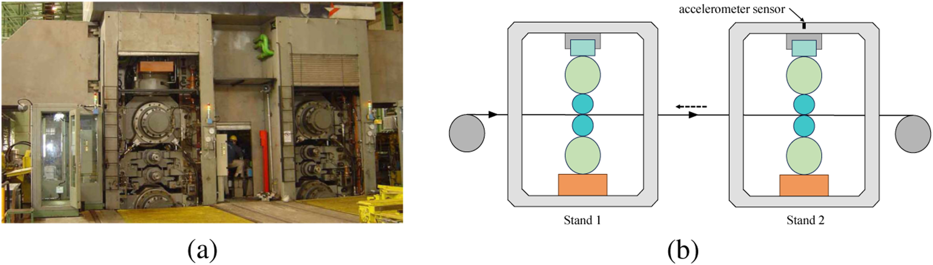

To achieve the maximum possible rolling speed and prevent strip rupture and equipment damage, a chatter detection system is employed. The chatter detection system employs data from the accelerometer sensor mounted on the top housing of the second stand. In Figure 1(b), the placement of the accelerometer sensor is illustrated.

The data acquisition frequency of the employed sensor is 5120 Hz. The vibration data is filtered within the frequency range of 70–140 Hz. The operation of the detection system is such that two levels of warning and alarm are calculated. If the root mean square (RMS) of the vibrations over the past 2 seconds exceeds the alarm level, and simultaneously, the RMS of the vibrations is increasing or a sudden increase in the RMS of the vibrations is detected, an alarm signal is issued. A warning signal is issued when the RMS of the vibrations over the past 2 seconds exceeds the warning level. The alarm level and the warning level are obtained according to equation (1).

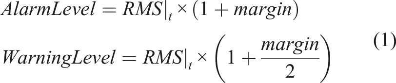
\begin{aligned} A l a r m L e v e l = R M S |_{t} \times (1 + m a r g i n) \\ W a r n i n g L e v e l = R M S |_{t} \times (1 + \frac{m a r g i n}{2}) \end{aligned}

(1)

RMS|_t represents the RMS of vibrations over the past t seconds. The margin is determined experimentally based on four parameters: strip thickness, strip width, work roll mileage (measured in kilometers), and rolling speed. For determine the alarm level under constant speed conditions, the RMS value of vibrations over the past 10 seconds is used and in conditions of increasing speed, and for up to 2 seconds afterward, the RMS value of vibrations over the past 4 seconds is used to avoid false alarms. The warning level is determined in a similar manner to the alarm level, with the exception that it is determined using half of the calculated margin for the alarm level. Figure 2 illustrates the functionality of the chatter detection system in the third pass of the rolling process of a coil.

Figure 2.

Functionality of the chatter detection system: (a) Variations of the linear speed for the second stand, and moments at the warning and alarm signals were issued; (b) Variations in the RMS values of vibrations, warning level, and alarm level.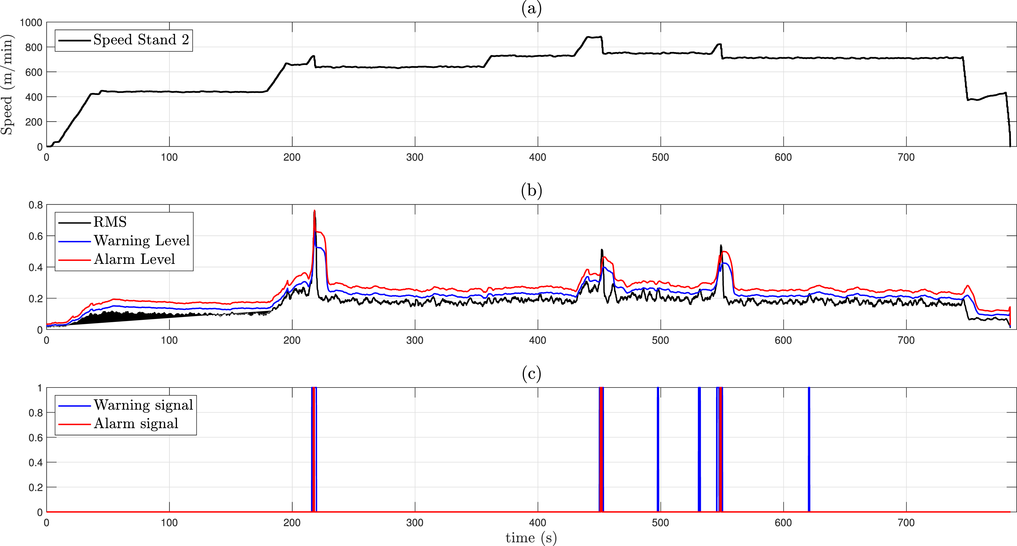

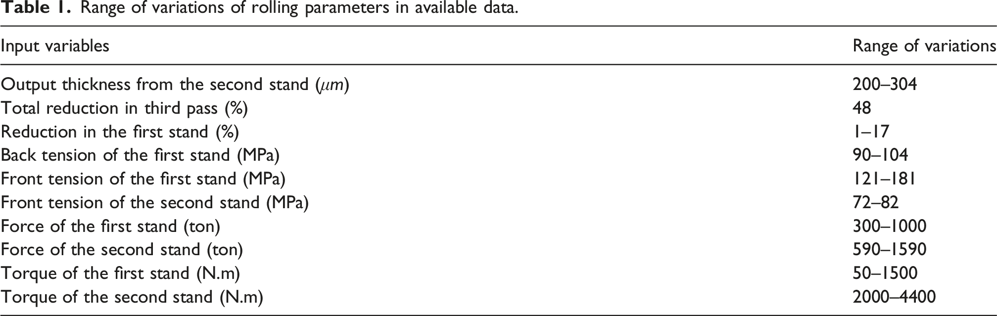
In this study, archived data from 188 various coils were utilized, which were acquired using a data acquisition system equipped with a hardware-level anti-aliasing filter to attenuate high-frequency components and prevent aliasing in the sampled signals. Since chatter occurs at high speeds and in thin strips, this study only utilizes data from the third rolling pass of strips having an output thickness less than 304 μm. Figure 3 illustrates the histogram of the output strip thickness from the second stand in the third rolling pass for all coils. In Table 1, the variation ranges of some rolling parameters in the available data are shown. In previous studies, the effects of these parameters on chatter occurrence speed have been investigated using mathematical and FEM (Kimura et al., 2003; Mehrabi et al., 2015). Analyzing the impact of these parameters on chatter occurrence speed was not an objective of the present study.

Figure 3.

The histogram of the output strip thickness from the second stand in the third rolling pass.

Table 1.

Range of variations of rolling parameters in available data.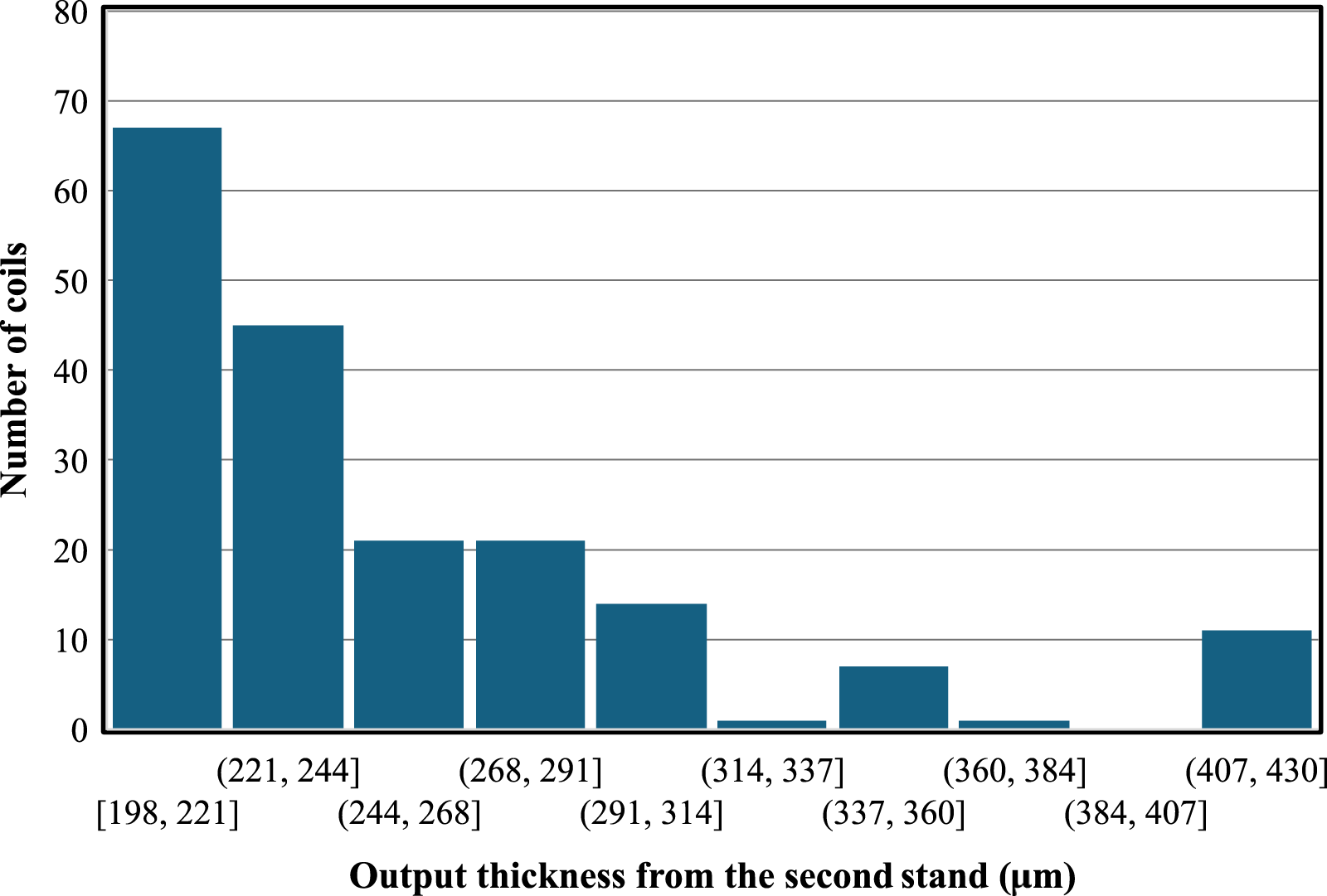

Input variables	Range of variations
Output thickness from the second stand (μm)	200–304
Total reduction in third pass (%)	48
Reduction in the first stand (%)	1–17
Back tension of the first stand (MPa)	90–104
Front tension of the first stand (MPa)	121–181
Front tension of the second stand (MPa)	72–82
Force of the first stand (ton)	300–1000
Force of the second stand (ton)	590–1590
Torque of the first stand (N.m)	50–1500
Torque of the second stand (N.m)	2000–4400

The proposed chatter detection system may issue alarm signals at very low speeds, and for this reason, it is assumed that if the rolling speed at the time of alarm is less than 300 m per minute, the alarm signal is a false alarm. In the chatter detection system, if the RMS value of the vibrations exceeds either the warning or alarm level, a warning or alarm signal is issued every 0.1 seconds, leading to the registration of multiple signals during the occurrence of chatter. For this reason, it is assumed that if the time between the issuing of two consecutive warning or alarm signals is less than 0.5 seconds, only the signal corresponding to the higher rolling speed is considered. If the time exceeds 0.5 seconds, two separate warning or alarm signals are considered. It is expected that with the issuance of the first alarm signal at a speed, the rolling speed should not be further increased to prevent chatter. To investigate this matter, the value of γ, defined as the ratio of the speed at which the alarm signal is issued to the maximum speed at which a coil has been rolled, was calculated. The closer γ is to 1, it indicates that the operator has not increased the machine speed after the issuance of the alarm signal. In Figure 4(a), the histogram of the number of alarm signals at values of γ for all coils is illustrated. It can be observed from Figure 4(a) that in many cases, despite the issuance of an alarm signal, the rolling speed has increased significantly.

Figure 4.

The histogram of (a) Number of alarm signals at values of γ for all coils; (b) Critical speeds of the second stand in the high-fidelity dataset created using γ = 0.6.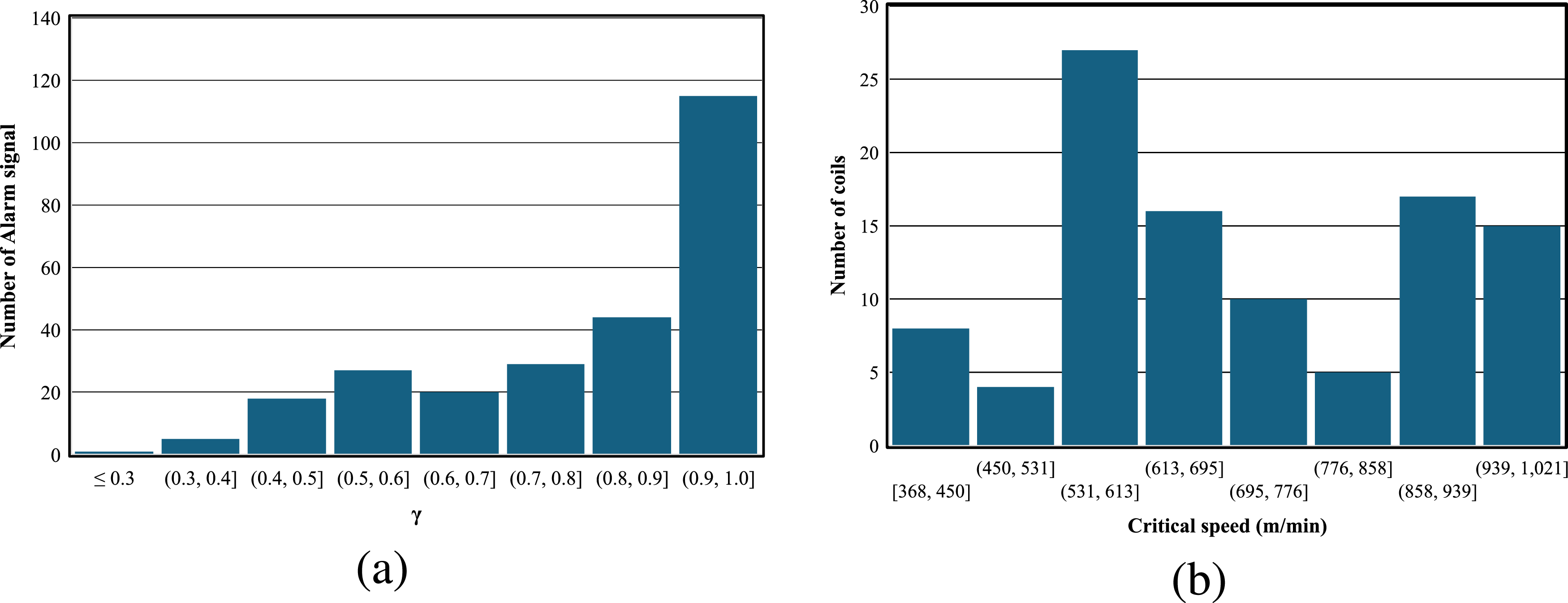

The chatter detection system may issue several alarm signals during the rolling of each coil. To prevent damage to the strip, a conservative approach is to consider the first alarm given by the chatter detection system as the occurrence of chatter. The problem with using this method is that the detection system may issue an alarm signal at speeds lower than those typically used for rolling. For this reason, to create a dataset, it is assumed that if γ for a coil is greater than 0.6, the minimum speed at which the alarm signal is issued is considered as the critical speed, whereas if γ is less than 0.6, the coil is not considered in the dataset. The reason for selecting a value of 0.6 is that if the operator determines that, despite receiving an alarm signal at a certain speed, the rolling speed can be increased to more than twice the speed at which the alarm signal was issued, it is likely that the signal was a false alarm and can be disregarded. Coils without an alarm signal are also excluded from the dataset. The histogram of critical speeds for the high-fidelity dataset created using the value of 0.6 is shown in Figure 4(b). The total number of high-fidelity data points is 102.

3. The low-fidelity dataset extracted from the rolling process simulation

In this section, the analytical model employed for simulating the rolling process is first introduced, and then the RSM and its application are explained.

3.1. The analytical model for simulating the rolling process

In this study, the analytical model of the two-stand cold rolling mill introduced in Section 2, has been utilized. This model was developed in the Simulink environment of MATLAB software in the study by Heidari et al. (2018). This model includes the payoff reel, dynamic model of first and second stands, and pickup reel. In the payoff reel and pickup reel models, the variations in the tension behind the first stand and in front of the second stand are considered. In the dynamic models of the first and second stands, the inter-stand tension, the stand structure model, and the rolling process model with Coulomb damping are considered.

The analytical model has been used to determine the critical speed at different values of the rolling parameters. The model is executed for different speeds at specific values of the rolling parameters, and the speed at which the vibration amplitude remains constant over time is considered the critical rolling speed. In each model execution, a 5-s segment of the rolling process is simulated. The 5-s duration was determined based on our parametric simulations at different time horizons, in conjunction with the reference plots reported by Heidari et al. (2018).

In Figure 5, the variations in the amplitude of oscillations of the second stand at different speeds are shown.

Figure 5.

The simulated vibrations of the second stand in the model for (a) At speeds lower than the critical speed, and (b) At speeds higher than the critical speed.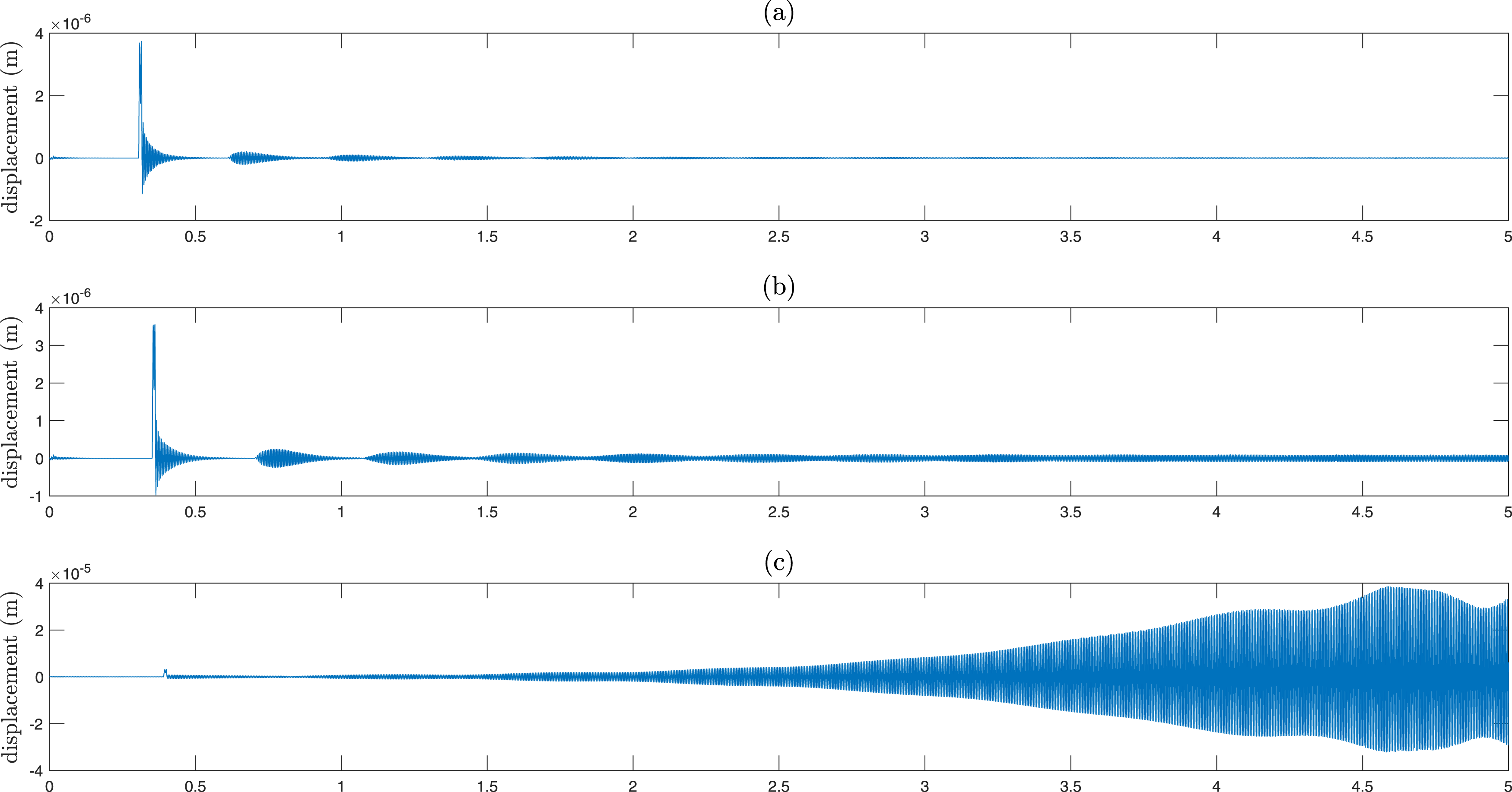

Each simulation of the rolling process for a duration of 5 seconds takes more than 90 minutes. Due to the time-consuming process of generating a dataset from the analytical model, the RSM was employed to establish a regression model that relates the input parameters of the model and the critical speed. This regression model is used to generate a large number of low-fidelity data points.

3.2. Response surface methodology

RSM is a collection of statistical and mathematical techniques useful for developing, improving, and optimizing processes. The most extensive applications of RSM are in the industry, particularly in situations where several input variables potentially influence performance measures or quality characteristics of the product or process (Myers et al., 2016).

In the RSM, it is assumed that the process, or system involves a response y that depends on the controllable input variables x₁, x₂, …, x_k. The relationship between the input variables and the output is expressed as equation (2).

y = f (x_{1}, x_{2}, \dots, x_{k}) + ϵ

(2)

f is the unknown response function, and ϵ includes effects such as measurement errors, sources of instability, and others on the response. ϵ is considered as a statistical error and is often assumed to follow a normal distribution with a zero mean and variance σ². Because the response function f is unknown, it is approximated. In many cases, a first-order or second-order model is used. In this study, a second-order model was used. The second-order model is given by equation (3) (Myers et al., 2016).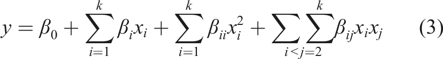

y = β_{0} + \sum_{i = 1}^{k} β_{i} x_{i} + \sum_{i = 1}^{k} β_{i i} x_{i}^{2} + \underset{i < j = 2}{\sum \sum^{k}} β_{i j} x_{i} x_{j}

(3)

where β₀, β_i, β_ii, and β_ij are the regression coefficients, while x_i and x_j represent the input variables. There are different methods or designs for selecting the levels of input parameters. These designs, by appropriately selecting points or levels, reduce the number of experiments needed for modeling. The selection of parameter levels is based on the central composite design (CCD). In the CCD, 5 levels are considered for each factor.

Due to the fact that determining the critical speed using the analytical model is a trial-and-error and time-consuming process, the RSM is used to establish a relationship between the rolling parameters and the critical speed of the analytical model. The RSM was implemented in Minitab software within the range of actual data variations. The parameters of the analytical model, including the reduction in the first stand, the output thickness from the second stand, the friction coefficients for the first and second stands, the back tension of the first stand, the front tension of the first stand, and the front tension of the second stand are considered as input variables. The critical speed is considered as the output or response. In Table 1, the ranges of the input variables are provided. The friction coefficients for all coils have been calculated using the analytical model. The coefficient of friction is determined by selecting the value that makes the force of the analytical model equal to the actual force. By averaging over all coils, the total reduction in third pass, strip width and the work roll radius of the first and second stands are found to be 48%, 782 mm, 236 mm, and 230 mm, respectively.

Using the CCD for 7 input variables, 143 experiments are required based on the n² + 2 × n + 1 formula. The critical speed of 143 experiments was obtained through trial and error of the analytical model at different speeds.

4. The proposed method for predicting the chatter critical speed

This section presents the neural networks trained using low-fidelity and high-fidelity data, as well as the neural network architecture employed for TL. In Figure 6, the schematic diagram of TL and direct DL is presented. In TL, Model A is first trained using low-fidelity data. Although Model A exhibits low accuracy, it is capable of learning the fundamental features and general patterns within the data. Model A is used as a pre-trained neural network, and through fine-tuning with high-fidelity data, Model B is obtained. Model C, is trained directly using high-fidelity data.

Figure 6.

Schematic diagram of TL and direct DL.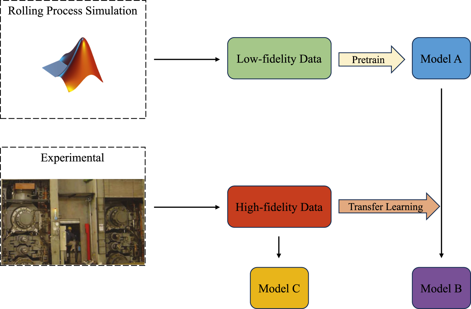

TL in ML refers to a technique where a model leverages knowledge gained from one or more source tasks to improve learning performance on a target task. An important aspect of the benefits of TL is in simulation technology (Yang et al., 2020). TL, when dealing with different levels of data fidelity, is an essential step to adapt to many situations that are not encountered in the simulated environment.

The TL network architecture used consists of two interconnected neural networks, NN_L and NN_H. This structure is illustrated in Figure 7. NN_L is the same as Model A, responsible for processing low-fidelity data. The output of this network, Q_L, encapsulates the overall behavior of the low-fidelity data and serves as the input to the NN_H network. The fine-tuning strategy is such that the trainability of certain layers in the NN_L section is deactivated, and the remaining layers are trained using high-fidelity data.

Figure 7.

Architecture of the transfer learning network (Model B): integration of low-fidelity (NN_L) and high-fidelity (NN_H) models.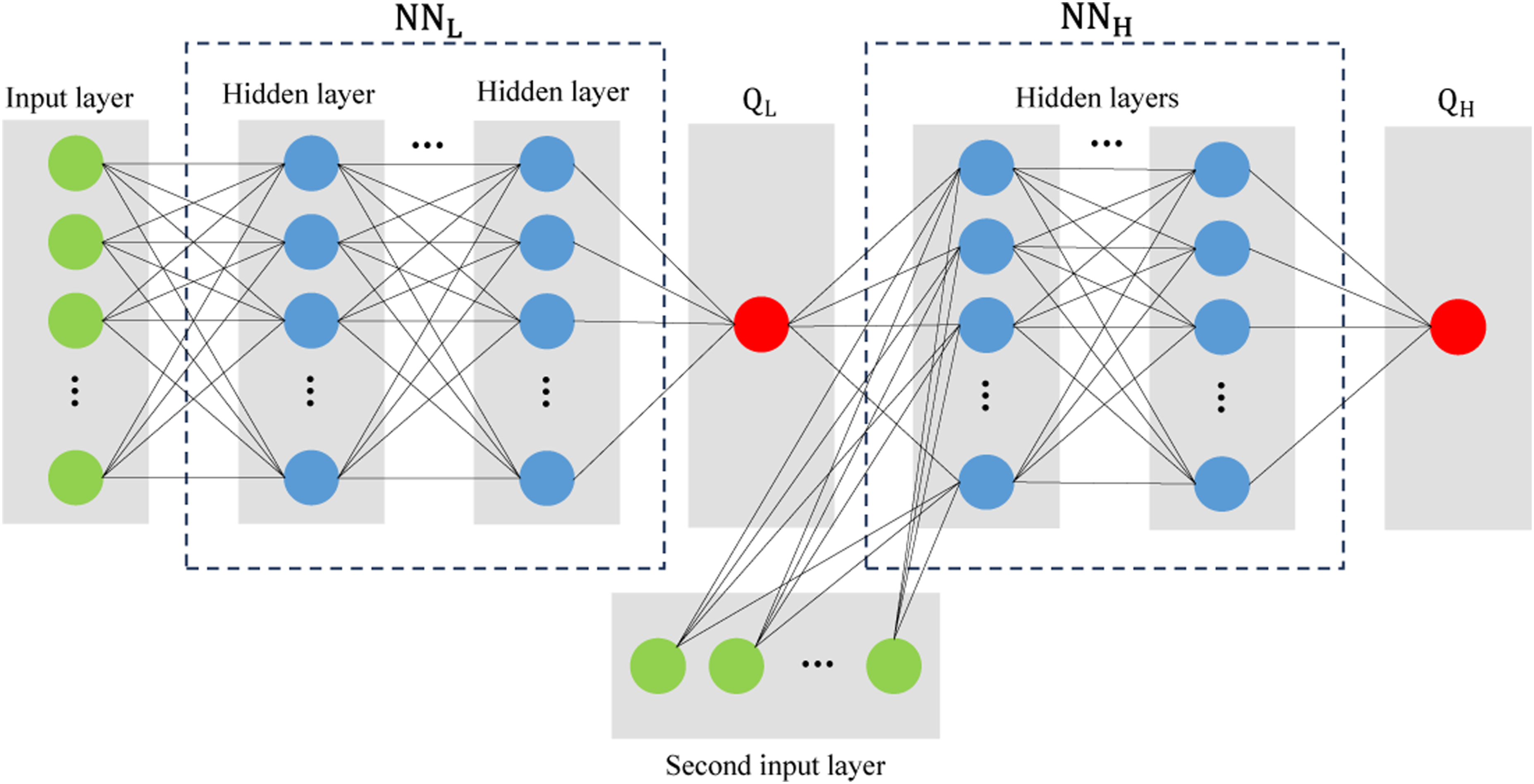

NN_H takes Q_L and some other parameters from the high-fidelity data as input and generates Q_H as the output. Adding the second input allows for capturing more complexities, while still leveraging the patterns identified from the low-fidelity data. As discussed in Section 1, rolling mills are complex systems, and various parameters influence the chatter phenomenon. The simplifications made in the development of simulation models result in not all influential parameters of the chatter phenomenon being considered, or some important parameters being regarded as dependent variables. Therefore, it is necessary to incorporate the important parameters that influence the occurrence of the chatter phenomenon and are not included in the first input, through the second input to the model.

In all models, Mean Squared Error (MSE) is used as the loss function, and the Stochastic Gradient Descent (SGD) optimizer with a momentum of 0.9 is employed. Regularization techniques and the EarlyStopping callback are employed to prevent overfitting.

5. Results and discussion

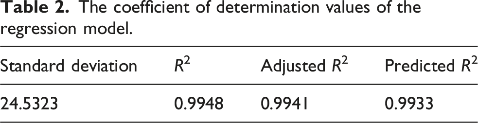
To evaluate the prediction performance of the regression models, the following metrics were used: the coefficient of determination (R²), the adjusted R², and the Root Mean Square Error (RMSE). The coefficient of variation (CV) was used to assess stability and sensitivity to data partitioning, while confidence intervals (CI) were employed to quantify uncertainty in the estimated performance metrics. The R² indicates the percentage of the variation in the dependent variable that is explained by the independent variables. The R² is obtained from equation (4).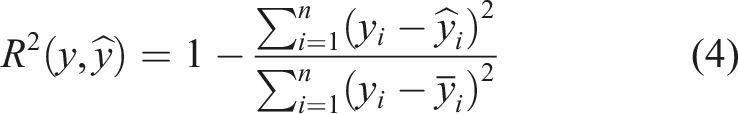

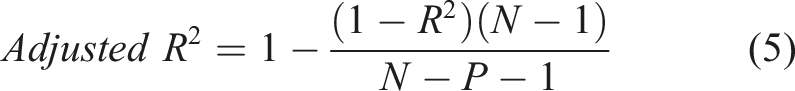
R^{2} (y, \hat{y}) = 1 - \frac{\sum_{i = 1}^{n} {(y_{i} - {\hat{y}}_{i})}^{2}}{\sum_{i = 1}^{n} {(y_{i} - {\bar{y}}_{i})}^{2}}

(4)

y_i is the actual value,

{\hat{y}}_{i}

is the predicted value, and

\bar{y} = 1 / n \sum_{i = 1}^{n} y_{i}

is the mean of the actual data. When a new parameter is added to a regression model, the R² increases, even if there is no actual improvement in the response of model. The adjusted R² is used to assess the true impact of the independent variables on the response. The adjusted R² is obtained from equation (5).

A d j u s t e d R^{2} = 1 - \frac{(1 - R^{2}) (N - 1)}{N - P - 1}

(5)

N represents the total number of data points, and P represents the number of independent variables.

RMSE is a way to measure the average magnitude of the differences between predicted values and observed values. Basically it’s quantifies how well a model is performing in predicting numeric outcomes. The value of the RMSE is obtained from equation (6).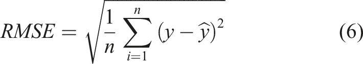

R M S E = \sqrt{\frac{1}{n} \sum_{i = 1}^{n} {(y - \hat{y})}^{2}}

(6)

The CV is defined as the ratio of the standard deviation to the mean. A p-CI is defined as an interval that includes the true performance of the model with (at least, if being conservative) probability p in identical repetitions of the analysis with new datasets from the same data distribution (Paraschakis et al., 2024). The CI was estimated using the percentile bootstrap method. In percentile bootstrap, the percentiles of the bootstrap sampling distribution are used to create a confidence interval, where the lower and upper bounds are taken from the 2.5% and 97.5% percentiles of the bootstrap distribution. Further details are presented by (Flowers-Cano et al., 2018).

5.1. The nonlinear regression developed for generating low-fidelity data

Using the RSM introduced in section 3.2, a nonlinear regression equation has been derived to describe the relationship between the input data of the analytical model and the chatter critical speed. The results of the RSM are shown in Table 2. These results are in the case where the variables with p-values greater than 0.05 have been excluded from the regression equation. The residual plots are shown in Figure 8.

Table 2.

The coefficient of determination values of the regression model.

Standard deviation	R ²	Adjusted R²	Predicted R²
24.5323	0.9948	0.9941	0.9933

Figure 8.

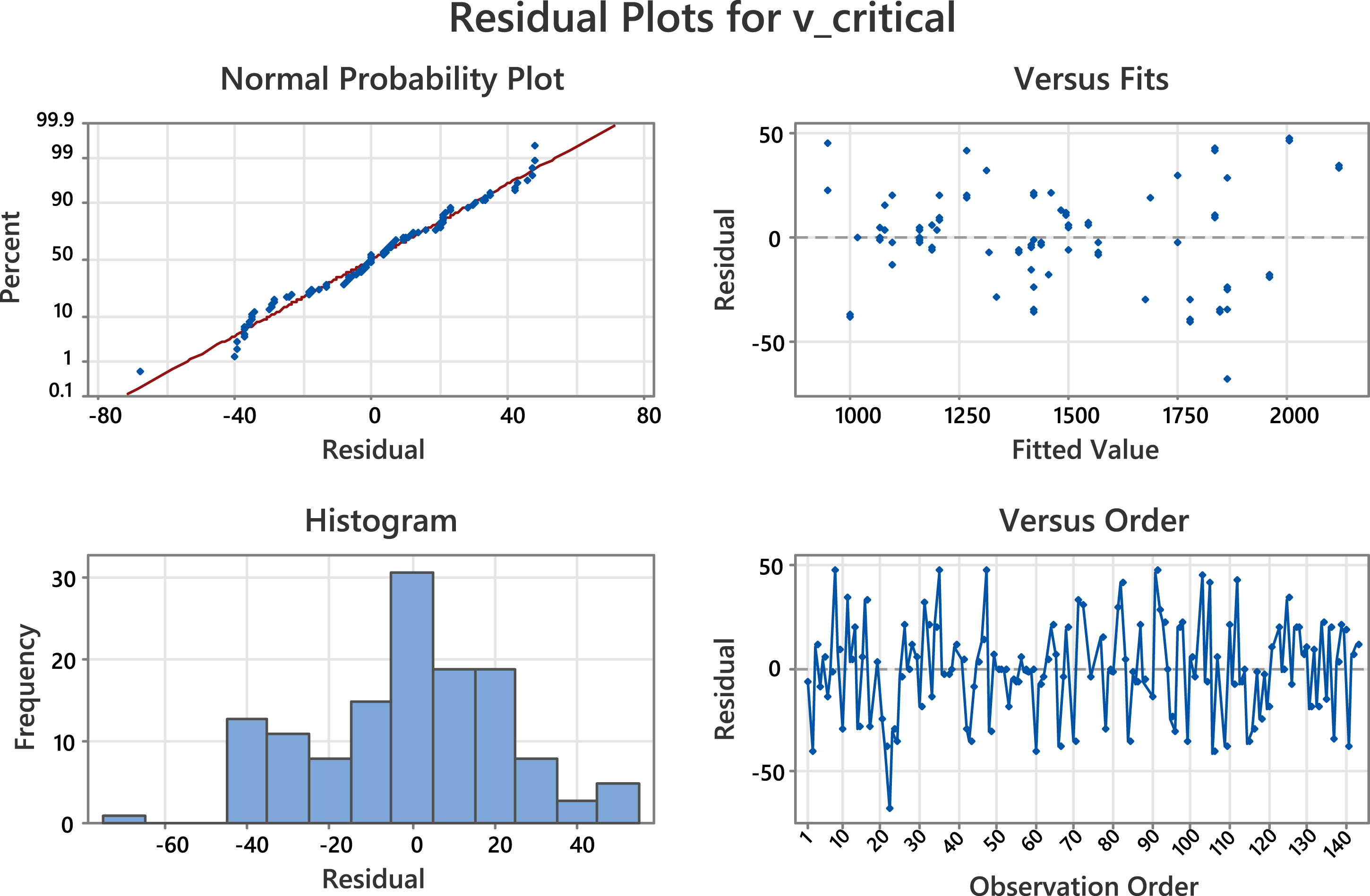
Residual plots for the regression model generated by the RSM.

The regression equation generated by the RSM is given in equation (7). The variables in this equation have been scaled to the range of −1 to +1.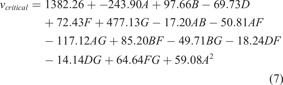

\begin{aligned} v_{critical} & = 1382.26 + - 243.90 A + 97.66 B - 69.73 D + 72.43 F + 477.13 G \\ - 17.20 A B - 50.81 A F - 117.12 A G + 85.20 B F - 49.71 B G \\ - 18.24 D F - 14.14 D G + 64.64 F G + 59.08 A^{2} \end{aligned}

(7)

In this equation, A is output thickness from the second stand, B is reduction in the first stand, D is front tension of the first stand, F is friction coefficients of the first stand, and G is friction coefficients of the second stand. As shown in equation (7), the variables related to the back tension of the first stand and the front tension of the second stand do not affect the calculation of the critical speed in the model. These two factors have been excluded from the equation due to their high p-values. In other words, a predictor with a low p-value is likely to have a significant effect on the response of model. The critical speed in equation (7) refers to the linear speed of the second stand in meters per minute. The simulation model takes the input strip speed to the first stand as an input. The linear speed of the first and second stands is equal to the strip speed at the neutral point.

In order to compare the critical speed obtained from the analytical model with the rolling speed of real data, data from 20 coils have been used. For each coil, the average value of each rolling parameter was calculated, and then the analytical model was run using these values to determine the obtained critical speed. Furthermore, the speeds predicted by the regression model are also calculated using these average values. The RMSE value for these data was obtained as 92.4. In Figure 9, the critical speeds obtained from both the analytical and regression models, as well as the maximum speed at which each coil was rolled are shown. As mentioned in section 2, high-fidelity data was obtained using the γ = 0.6. This leads to larger difference between the critical speeds of the low-fidelity data and the actual chatter speed in high-fidelity data, compared to the difference shown in Figure 9. Therefore, to reduce the difference between the critical speeds of low-fidelity data and high-fidelity data, the critical speeds calculated from the regression model are divided by the correction factor. The correction factor is calculated as follows: for high-fidelity data. The critical speed is determined using the regression equation. The ratio of the critical speed of regression model to the critical speed of the high-fidelity data is then computed, and the average of this ratio is taken across all the data. The correction factor for the high-fidelity data created with γ = 0.6 is 1.8878.

Figure 9.

Comparison of the critical speed obtained from the analytical model and regression model with the maximum rolling speed for 20 different coils.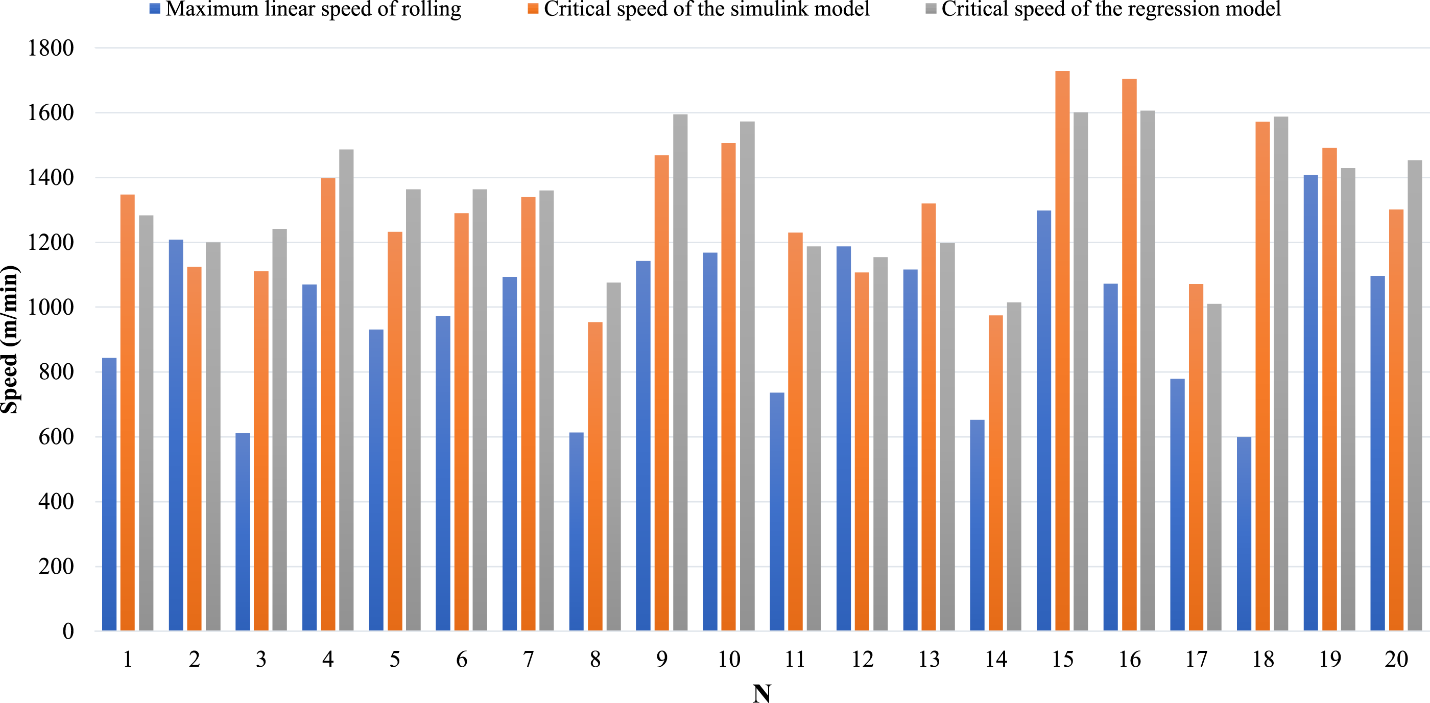

5.2. Prediction performance of direct DL (Model C) and TL (Model B) on high-fidelity dataset

A low-fidelity dataset is generated using the regression model developed between the input parameters and the output of the analytical model. Seven levels are selected within the range of input parameters (Table 1), which affect the calculation of the critical speed equation (7) and a low-fidelity dataset is generated using the full factorial design. The critical speeds for this dataset are calculated using the regression equation developed. Model A consists of three layers, with 16, 8, and 4 neurons in each layer, respectively. This model employs the LeakyReLU activation function with a negative slope of 0.1, Dropout with a rate of 0.2, and L2 regularization with a value of 0.0001. Model A is trained using 80% of the low-fidelity dataset and tested on the remaining 20%. The results indicate that the Model A has a R² of 0.999 on both the training and testing datasets.

The K-fold cross-validation technique is utilized for hyperparameter tuning. Initially, 0.15% of the high-fidelity data is set aside for final evaluation, while the remaining data is split into 6 folds for cross-validation. The number of hidden layers in Model C and in the NN_H section of Model B is set to 2. In the final layer of Models B and C, L2 regularization with a value of 0.01 is applied, while L1 regularization with the value of 0.001 is used in the intermediate layers of Model C and the NN_H section of Model B. The optimal values for the remaining hyperparameters are determined through random search. Table 3 presents the range of these hyperparameters.

Table 3.

Hyperparameter ranges for Model B and Model C for random search optimization.

Hyperparameter	Model B	Model C
Number of units	4, 5, 6, 7, 8, 9, 10	4, 5, 6, 7, 8, 9, 10
Dropout	0.05, 0.1, 0.15, 0.2, 0.25	0.05, 0.1, 0.15, 0.2, 0.25
Learning rate	(8, 10, 20) × 10⁻⁶	(8, 10, 20) × 10⁻⁶
Negative slope in LeakyReLU	0.0, 0.05, 0.1, 0.15, 0.2	0.0, 0.05, 0.1, 0.15, 0.2
Frozen layers	3, 4, 5	N/A

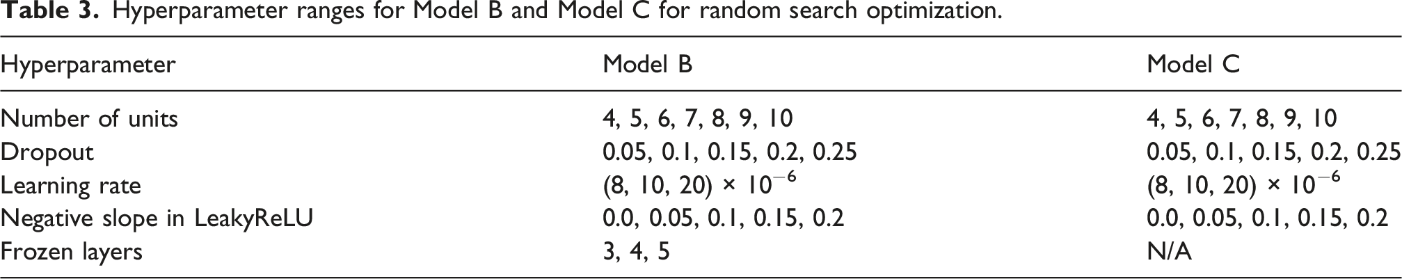
The second input layer in Model B includes the second stand torque, the work roll mileage of the second stand, which is equivalent to the roll surface roughness, the slip at the front of the second stand roll, the gap distance between the rolls of the second stand, front tension of the second stand, rolled length of strip, reduction in the second stand, and output thickness from the second stand. The input layer in Model C includes all the input parameters of Model B, except that instead of the friction coefficients for the first and second stands, the forces of the first and second stands are used. Additionally, between the parameters reduction in the first and second stand, only the reduction in the first stand is used.

For Model B, the best results for the hidden layers of the NN_H section have been obtained with neuron counts of 6 and 4, dropout rates of 0.1 and 0.15, and negative slopes of 0.15 and 0.1 in the LeakyReLU activation function. The learning rate and the number of frozen layers have been determined to be 8 × 10⁻⁶ and 5, respectively. In Figure 10(a), the cross-validation results of Model B have been presented. For this model, the average R² and the average RMSE for the training data are 0.745 and 93.5, respectively, while for the validation data, they are 0.734 and 89.8, respectively, with CV of 10% for R² and 16% for RMSE.

Figure 10.

The evaluation results of the (a) Model B, and (b) Model C using coefficient of determination, and root mean squared error.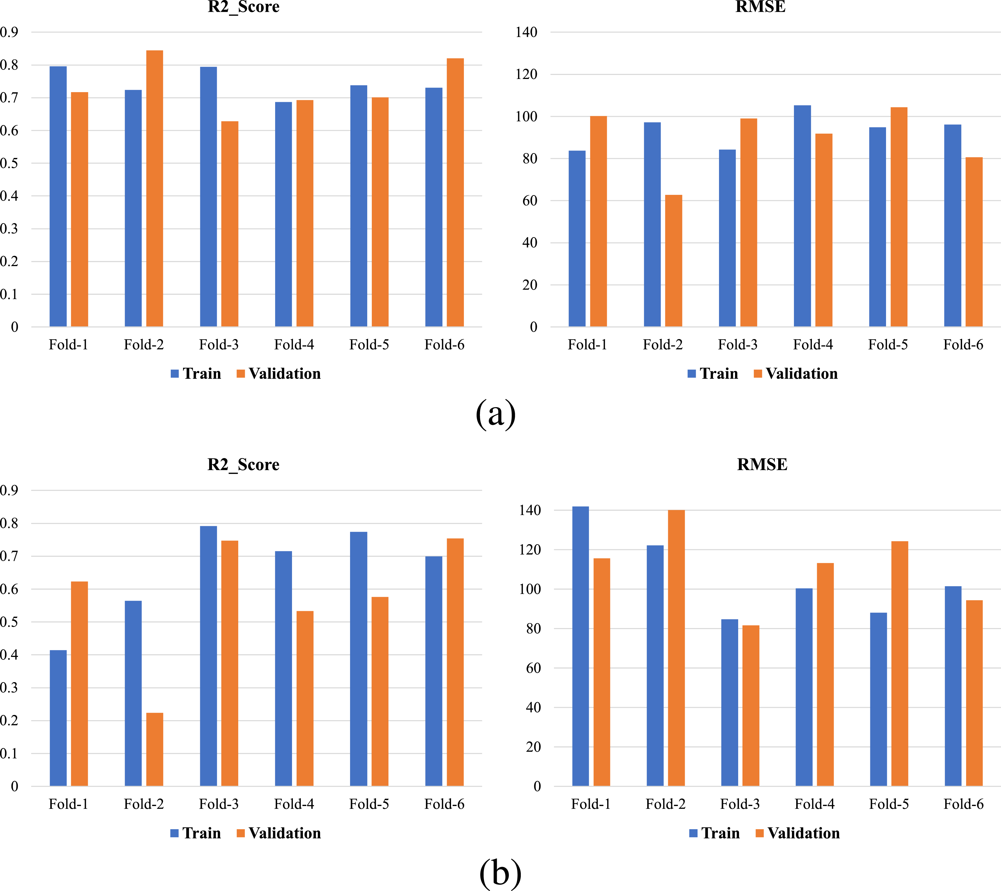

For Model C, the best results have been obtained with neuron counts of 4 and 4, dropout rates of 0.05 and 0.15, and negative slopes of 0.0 and 0.2 in the LeakyReLU activation function. The learning rate has also been determined to be 1 × 10⁻⁵. In Figure 10(b), the cross-validation results of Model C have been presented. For this model, the average R² and the average RMSE for the training data are 0.656 and 106.4, respectively, while for the validation data, they are 0.576 and 111.5, respectively, with CV of 30% for R² and 17% for RMSE. Comparison of the CV values of Models B and C shows that Model B is less sensitive to the training/test split.

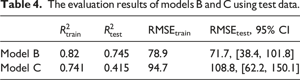
For the final evaluation of models B and C, data from all six generated folds have been used for model training. Table 4 presents the results of these models on the training and test data. The R² for models B and C on the test data are 0.74 and 0.41, respectively. Model B exhibits a greater R², lower RMSE and narrower CI on the test data, indicating that its predictions are more accurate and more stable than those of Model C. In Figure 11, the residuals are plotted against the actual speed values. Residuals are the difference between the predicted values and observed values.

Table 4.

The evaluation results of models B and C using test data.

	$R_{train}^{2}$	$R_{test}^{2}$	RMSE_train	RMSE_test, 95% CI
Model B	0.82	0.745	78.9	71.7, [38.4, 101.8]
Model C	0.741	0.415	94.7	108.8, [62.2, 150.1]

Figure 11.

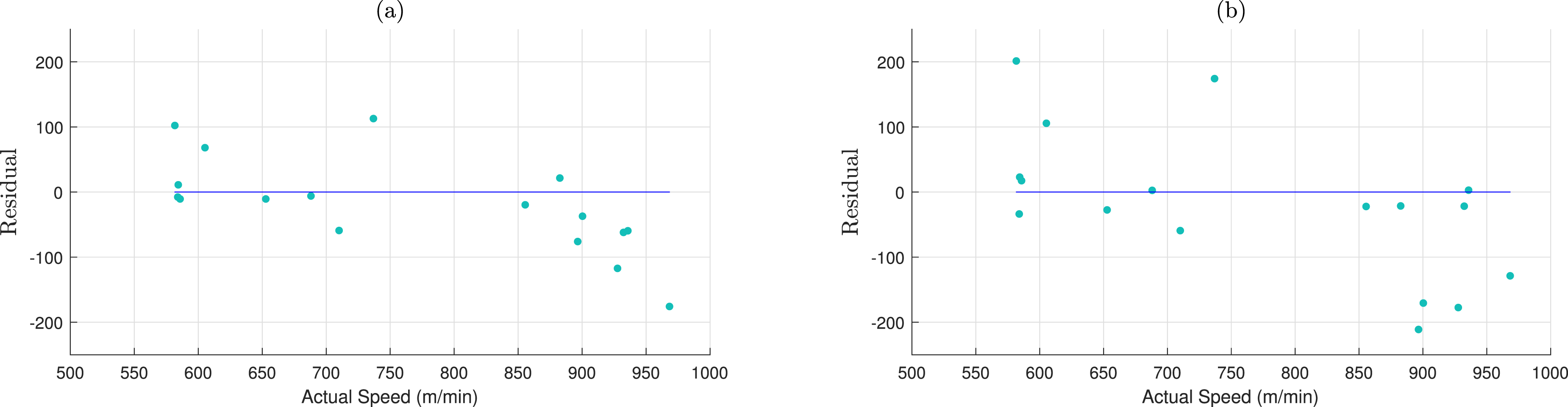
Residual plots against the actual speed values of test data for (a) Model B, and (b) Model C.

6. Conclusion

In order to perform high-speed and stable rolling, the critical chatter speed was predicted using MFTL. An analytical model developed in previous studies was used to generate the low-fidelity dataset. Due to the time-consuming nature of generating a dataset using the analytical model, the RSM was employed to establish a relationship between the input and output parameters of the model. Using this established relationship, a low-fidelity dataset has been generated, and used for initial model pre-training. High-fidelity dataset was created from the available real data based on the speeds at which the alarm signal occurred. Model B was developed using the TL approach, while Model C was created solely based on high-fidelity data. The results indicated that Model B and Model C achieved a R² of 0.74 and 0.41, respectively, on the test data. Thus, Model B demonstrated superior performance. The training time required for Model B is greater than that for Model C. However, because acquiring a sufficiently large dataset is a highly costly and time-consuming process, and industrial plants typically cannot provide such extensive data, a multi-fidelity framework was adopted to improve performance metrics and enhance result stability.

Footnotes

Acknowledgments

The authors express their gratitude for the cooperation of the experts in the cold rolling mill unit at MSC.

ORCID iDs

Ali Loghmani

Sayed Jalal Zahabi

Funding

The authors disclosed receipt of the following financial support for the research, authorship, and/or publication of this article: This work was supported by the Mobarakeh Steel Company (No. 48557056). The National Research Foundation of Korea(NRF) grant funded by the Korea government(MSIT) (No. RS-2025-25435356).

Declaration of conflicting interests

The authors declared no potential conflicts of interest with respect to the research, authorship, and/or publication of this article.

Data Availability Statement

The datasets generated during and/or analyzed during the current study are available from the corresponding author on reasonable request.*

References

An Khang

Wahab

Lee

(2025) Simultaneous imposition of initial and boundary conditions via decoupled physics-informed neural networks for solving initial-boundary value problems. Applied Mathematics and Mechanics 46: 763–780. https://doi.org/10.1007/s10483-025-3240-7

Flowers-Cano

Ortiz-Gómez

León-Jiménez

, et al. (2018) Comparison of bootstrap confidence intervals using monte carlo simulations. Water 10: 166. https://doi.org/10.3390/w10020166

Gao

Liu

Zhang

, et al. (2020) Chatter model with structure-process-control coupled and stability analyses in the cold rolling system. Mechanical Systems and Signal Processing 140: 106692. https://doi.org/10.1016/j.ymssp.2020.106692

Gao

Tian

Liu

, et al. (2021) Dynamics-based optimization of rolling schedule aiming at dual goals of chatter suppression and speed increase for a 5-stand cold tandem rolling mill. Journal of Iron and Steel Research International 28: 168–180. https://doi.org/10.1007/s42243-020-00551-5

Guo

Wang

Han

, et al. (2025) A deep neural network model for parameter identification in deep drawing metal forming process. Journal of Manufacturing Processes 133: 380–394. https://doi.org/10.1016/j.jmapro.2024.11.067

Heidari

Forouzan

(2013) Optimization of cold rolling process parameters in order to increasing rolling speed limited by chatter vibrations. Journal of Advanced Research 4: 27–34. https://doi.org/10.1016/j.jare.2011.12.001

Heidari

Forouzan

Niroomand

(2018) Development and evaluation of friction models for chatter simulation in cold strip rolling. The International Journal of Advanced Manufacturing Technology 96: 1–21. https://doi.org/10.1007/s00170-018-1658-x

Hou

Cheng

Zhang

, et al. (2025) Fault diagnosis and classifications of rolling mill bearing-gear based on gadf-tl-shufflenet-v2. Journal of Vibration and Control 0(0): 10775463251336975. https://doi.org/10.1177/10775463251336975

Kimura

Sodani

Nishiura

, et al. (2003) Analysis of chatter in tandem cold rolling mills. ISIJ International 43(1): 77–84. https://doi.org/10.2355/isijinternational.43.77

10.

Kocabıçak

Wang

Han

, et al. (2025) A deep neural network approach to predict dimensional accuracy of thin-walled tubes in backward flow forming plasticity process. Journal of Manufacturing Processes 141: 59–80. https://doi.org/10.1016/j.jmapro.2025.02.044

11.

Zhang

, et al. (2022) On-line transfer learning for multi-fidelity data fusion with ensemble of deep neural networks. Advanced Engineering Informatics 53: 101689. https://doi.org/10.1016/j.aei.2022.101689

12.

Liang

Liu

, et al. (2023) A novel efficient probabilistic prediction approach for train-induced ground vibrations based on transfer learning. Journal of Vibration and Control 30: 576–587. https://doi.org/10.1177/10775463221148792

13.

Liu

Jiang

Luo

(2022) Leveraging low-fidelity data to improve machine learning of sparse high-fidelity thermal conductivity data via transfer learning. Materials Today Physics 28: 100868. https://doi.org/10.1016/j.mtphys.2022.100868

14.

Sun

Song

, et al. (2020) Prediction and analysis of cold rolling mill vibration based on a data-driven method. Applied Soft Computing 96: 106706. https://doi.org/10.1016/j.asoc.2020.106706

15.

Luan

Zhang

(2024) Multi-fidelity transfer learning for complex bund overtopping prediction with varying input dimensions. Journal of Loss Prevention in the Process Industries 92: 105477. https://doi.org/10.1016/j.jlp.2024.105477

16.

Mehrabi

Salimi

Ziaei-Rad

(2015) Finite element analysis on chattering in cold rolling and comparison with experimental results. Journal of Manufacturing Science and Engineering 137(6): 061013. https://doi.org/10.1115/1.4030379

17.

Myers

Montgomery

Anderson-Cook

(2016) Response Surface Methodology: Process and Product Optimization Using Designed Experiments. Wiley Series in Probability and Statistics. https://books.google.com/books?id=T-BbCwAAQBAJ

18.

Nagai

Nohara

(2023) Chattering Detection Method for Cold Rolling Mill, Chattering Detection Device for Cold Rolling Mill, Cold Rolling Method, and Cold Rolling Mill. US Patent 11,779,978 B2. U.S. Patent and Trademark Office. https://patents.google.com/patent/US11779978B2/fr

19.

Niroomand

Forouzan

Salimi

, et al. (2012) Frequency analysis of chatter vibrations in tandem rolling mills. Journal of Vibroengineering 14: 852–865.

20.

Niroomand

Forouzan

Heidari

(2019) Experimental analysis of vibration and sound in order to investigate chatter phenomenon in cold strip rolling. The International Journal of Advanced Manufacturing Technology 100: 673–682. https://doi.org/10.1007/s00170-018-2639-9

21.

Noh

Solichin

Kim

(2023) Enhancing realistic remaining useful life prediction using multi-fidelity physic-informed neural network approach. Annual Conference of the PHM Society 15: 1. https://doi.org/10.36001/phmconf.2023.v15i1.3474

22.

Paraschakis

Castellani

Borboudakis

, et al. (2024) Confidence interval estimation of predictive performance in the context of automl. https://arxiv.org/abs/2406.08099

23.

Pattnaik

Shrivastava

Parvathi

(2020) Transfer learning-based framework for classification of pest in tomato plants. Applied Artificial Intelligence 34(13): 981–993. https://doi.org/10.1080/08839514.2020.1792034

24.

Shi

Liu

Xue

, et al. (2024) Prediction of supercritical co2 heat transfer behaviors by combining transfer learning and deep learning based on multi-fidelity data. International Journal of Heat and Mass Transfer 218: 124802. https://doi.org/10.1016/j.ijheatmasstransfer.2023.124802

25.

Wang

Gao

Xin

(2023) Multi-step-ahead prediction of cold rolling chatter state based on the combination of functional data analysis and general autoregression model. SN Applied Sciences 5: 137. https://doi.org/10.1007/s42452-023-05353-4

26.

Yang

Zhang

Dai

, et al. (2020) Transfer Learning. Cambridge University Press. https://books.google.com/books?id=CLyDxgEACAAJ

27.

Yun

Wilson

Ehmann

(1998) Review of chatter studies in cold rolling. International Journal of Machine Tools and Manufacture 38(12): 1499–1530. https://doi.org/10.1016/S0890-6955(97)00133-8

28.

Zhang

Yang

, et al. (2024) A multi-fidelity transfer learning strategy based on multi-channel fusion. Journal of Computational Physics 506: 112952. https://doi.org/10.1016/j.jcp.2024.112952

29.

Zhang

Wang

, et al. (2025) Machinery fault diagnosis based on a transfer learning model with local sparse structure of pmdcnn-lstm. Journal of Vibration and Control 32: 1497–1513. https://doi.org/10.1177/10775463251315798