Modeling Urban Neighborhood Violence: The Systemic Model and Variable Effects of Social Structure

Introduction

The systemic model of social disorganization has proven valuable to community criminology in demonstrating how social structure conditions the informal and formal capacities of communities to regulate violent crime (Bursik and Grasmick 1993; Taylor 2015). Empirical literature on the systemic model has focused on explaining the linkages between three structural conditions and neighborhood violence: disadvantage, residential turnover, and ethnoracial composition.

Disadvantage undermines the ability of residents to exert informal social control needed to protect against violence. Furthermore, disadvantaged environments may be characterized by high levels of residential turnover (Bursik 1999). As such, the high mobility of residents renders it difficult to establish agreed-upon norms and to develop the social and political capital necessary to solicit resources from city-level agencies that can formally regulate deviance (Bursik and Grasmick 1993; Slocum et al. 2013). Instability is also associated with large swaths of vacant housing and disinvestment—conditions possibly indicative of neighborhood desirability, but arguably are related to local violence (Kane and Cronin 2013; Vélez and Richardson 2012; Yonas, O’Campo, Burke, et al. 2007). Equally concerning is that persistent socioeconomic isolation endemic to extremely disadvantaged communities can lead to adaptations that are amenable to violence (Anderson 1999; Majors and Billson 1993; Martin, McCarthy, Conger, et al. 2011; Stewart and Simons 2006).

Additional empirical contributions show that the occurrence of violence in adjacent neighborhoods also bears association with focal neighborhood violence (Pattillo 1998; Sampson 2012). Thus, violent conflicts occurring in focal neighborhoods have the potential to spillover to adjacent communities, and vice versa. But, because neighborhoods are stratified on their exposures to social structural conditions, they too are stratified on their exposures to violent spillover effects (Peterson and Krivo 2010). Generally, predominately White neighborhoods are spatially proximate to communities with low levels of disadvantage and violence, while predominately Black neighborhoods tend to be situated within clusters of communities characterized by high levels of disadvantage and violence (Peterson and Krivo 2010). This differential exposure to nearby social dislocations then leaves Black neighborhoods more vulnerable than White neighborhoods to the violence-inducing effects of nearby communities (Peterson and Krivo 2010).

Although the systemic model provides a way by which to understand structure-neighborhood violence linkages, current tests of the model are limited in that they treat neighborhoods of largely different violence levels as ecologically similar (Johnson and Kane 2018). For example, it is possible that residential turnover has very little effect on low to average violence neighborhoods, but could be extremely problematic in high-violence neighborhoods where additional flight could denigrate needed capacity for informal social control. Similarly, disadvantage could have a stronger effect on violence in low-violence neighborhoods. But, in higher violence neighborhoods, a ceiling effect may occur as violence levels are already so high that an increase in disadvantage is inconsequential (Hipp and Yates 2011).

In this study, I demonstrate that the effects of key structural correlates of the systemic model are variable across different segments of a neighborhood violent crime distribution. Lending support to prior studies, I find that the effect of structural disadvantage is weaker at higher quantiles of the violence distribution. At the same time, measures of residential instability, the concentration of unoccupied housing units, and the spatial proximity to other violent neighborhoods strengthen from lower to higher quantile models. In addition, I find that these effects are conditioned by local racial composition. While some work has considered some of these issues before, none has modeled the multiple distributional effects of these measures simultaneously. To address this gap, I use quantile regression to model the effects of violence in adjacent neighborhoods and social structure at select quantiles of a violent crime distribution. In doing so, I also account for different race-based sociohistorical contexts by performing parallel analyses of majority Black and White neighborhoods. Below, I begin by conceptually framing this argument considering existing literature. I then describe the study’s methodology and results, and conclude with a discussion of theoretical and policy implications.

The Systemic Model

The systemic model predicts that structural conditions can influence the extent of networks within neighborhoods and between neighborhoods and local/municipal organizations to demonstrate regulatory capacity at the private, parochial, and public levels of social control (Bursik and Grasmick 1993; Hunter 1985). Theoretically, each level of social control contributes independently and collectively to neighborhood social order. Empirical research demonstrating the linkages between such social orders and local crime spans several decades.

Local regulation that emanates from private order remains a theme of criminological research at the neighborhood level. The systemic model argues that local structural conditions can influence the ability of primary relational networks to regulate the behaviors of residents and visitors, especially children. This is because the family is a critical institution responsible for the informal socialization of children into law-abiding behavior (Messner and Rosenfeld 2007). Substantial research has demonstrated that low levels of attachment between parents and children yield behavioral consequences of low self-control and potentially crime (Gottfredson and Hirschi 1990). Conversely, higher levels of attachment are associated with the internalization of prosocial values and the avoidance of behaviors that undermine parental expectations (Hirschi 1969). Some scholars have noted that economic shifts may influence family structures in ways that have implications for child socialization and delinquency. For example, Wilson (1987) argued that the concentration of single parent households in urban underclass neighborhoods was due to the absence of employed, “marriageable” men. But, in the relative absence of traditional, nuclear family structures, elderly men and women may play a critical role in the supervision of neighborhood children (Anderson 1999).

At the parochial level, informal control occurs through network acquaintances that may or may not be grounded in friendship (Warner and Rountree 1997), including neighborly ties that enable the development of common expectations for behavior. Some scholars have found that parochial order in some places is associated with lower levels of burglary (Capowich 2003), Federal Bureau of Investigation (FBI) index crimes (Hawdon and Ryan 2009), and violence (Browning et al. 2017; Moore and Recker 2016). Another thread of research has found parochial relational network effects to intersect with local racial composition. For example, studies of crime in stable, working- and middle-class African-American Chicago neighborhoods have reported strong intraneighborhood ties but an ambivalence about reporting criminal and deviant behavior (Pattillo 1998; St. Jean 2007). Therefore, while residential stability can facilitate strong parochial relational ties, those ties may intertwine law abiding and criminal networks and, in turn, reduce regulatory capacity (Browning, Feinberg, and Dietz 2004). Additional studies have called into question the use of neighborhoods as units of analysis for measuring parochial order and have instead advocated the use of street blocks (Mazerolle, Kadleck, and Roehl 1998; Taylor 1997).

Public order occurs through the ability of neighborhood institutions and organizations to solicit crime control resources from municipal agencies. This element of the systemic model taps into a political economy perspective of urban neighborhoods by noting that neighborhoods vary in their abilities to acquire external resources, and that external investment is vital to neighborhood vitality. In a study of South Bronx, NY, Slocum et al. (2013) found that block groups with community organizations that garner and distribute social welfare resources to residents experienced less crime than those with organizations of other types. St. Jean’s (2007) qualitative study of poor, African-American Chicago neighborhoods found that unreliable public sanitation services and the failure of the city to secure vacant and derelict properties contributed to signs of disorder and crime. Other forms of external investment are significant as well. Studies have found that neighborhoods with higher financial investments in the form of approved home mortgage loans also experience lower crime rates (Vélez, Lyons, and Boursaw 2012; Vélez and Richardson 2012).

Although the systemic model assumes that the effects of social structure on violence are mediated through social networks and affiliated private, parochial, and public order mechanisms, only the social structure–violence relationship is directly investigated here. The appeal of the systemic model is that it provides a theoretical framework for which to understand how social structure effects (namely stability, socioeconomic status, and ethnoracial composition) can be interpreted (Johnson, Taylor, and Groff 2015). Those pathways are explored below.

Communities and crime scholars have argued that the amount of time spent in a neighborhood serves as a precursor to the development of mutual solidarity, attachment, and eventually regulation (Kasarda and Janowitz 1974; Warner and Rountree 1997). Relatedly, studies have noted the ways in which social ties and trust structure intra-neighborhood relations, relations with municipal agencies, and collective action against violence and antisocial behavior (St. Jean 2007; Warner, Swartz, and Hawk 2015). Thus, in line with the systemic model, not only does residential instability undermine the development of social ties needed for collective action against local violence, but it also renders neighborhoods increasingly vulnerable to violent spillover effects from adjacent neighborhoods.

There is also reason to believe that residential stability can be problematic for neighborhood regulation of violent crime (Pattillo 1998). Some scholars believe that long-term neighborhood residency, combined with social and spatial marginalization, breeds a distrust of law enforcement that is conducive to violent behavior (Anderson 1999; Sampson and Bartusch 1998; Wilson 1987). Accordingly, violence and the threat of violence emerges as a form of informal social control in settings of institutional neglect, supplanting the criminal justice system and crime control benefits derived from conventional neighborly ties. And, research shows that interactional dynamics between and among law abiding and non-law abiding residents are structured by what has been described as a “code of the street” (Anderson 1999), in spite of the code’s inability to provide measurable safety benefits (Stewart, Schreck, and Simons 2006). In light of conflict, both groups become less likely to call the police and instead rely more on violence to protect oneself and prevent violence (Duck 2015; Rosenfeld, Jacobs, and Wright 2003). More recent research has described some of these dynamics as legal cynicism—a neighborhood-level cultural frame of criminal justice institution distrust, precipitated by experiences of extreme socioeconomic disenfranchisement and the witnessing of negative interactions with the police (Desmond, Papachristos, and Kirk 2016; Kirk and Papachristos 2011).

Taken together, the current literature suggests that stability effects vary by local context. Although some work indicates that long-term residential stability inhibits the development of norms necessary to regulate violence, other work describes stability as helpful to local community regulation. A local context left unexplored, however, is violence. Stated differently, it is possible that residential stability effects are more pronounced in the most violent neighborhoods, as compared with mid-range and low-violence neighborhoods. This is because the most violent neighborhoods are likely characterized by a fear of crime that is so severe that it necessitates flight—further eroding regulatory capacity. On the contrary, instability effects in the least violent neighborhoods are potentially less problematic if there are local mechanisms of community norms and regulation to suppress crime. Scholarship lends some support to this hypothesis. Morenoff and Sampson (1997) examined the extent to which violent crime influenced changes in Black and White populations among Chicago census tracts from 1970 to 1990. Results indicated that Black populations decreased the most in neighborhoods with the highest homicide rates, which tended to be located at the spatial core of the ghetto. The greatest increases in Black population were noted in surrounding tracts where violence levels were increasing. White populations declined in tracts that demonstrated increases in homicide and those that were adjacent to increasingly violent tracts.

Although the connection between stability and neighborhood violence is inconsistently supported, scholars across generations have demonstrated the deleterious effects of neighborhood disadvantage on violence (Bursik 1986; Bursik and Webb 1982; Peterson and Krivo 2010; Sampson and Groves 1989; Sampson, Raudenbush, and Earls 1997; Shaw and McKay 1942; Taylor and Covington 1988). But, while structural disadvantage continues to be among the most reliable predictors of local violence (Hipp 2016; Pratt and Cullen 2005), its effects become dampened in communities characterized by extreme levels of violence.

Research on race-disaggregated homicide has found that the effect of concentrated disadvantage on violence depends on local racial composition. This group of studies has noted divergent and dire structural conditions of urban Black versus White neighborhoods and adaptations to conditions that are ripe for violence (Berthelot, Brown, Thomas, et al. 2016; Krivo, Peterson, and Kuhl 2009; Ousey 1999; Parker and McCall 1999; Sampson and Wilson 1994; Sampson 2009a). A vast body of research empirically demonstrates social and economic inequalities among urban neighborhoods (Briggs 2005; Massey and Denton 1993; Omori 2017). Historically, macro-structural shifts of de-industrialization led to increased demand for highly skilled labor at the expense of low-skill manufacturing positions that were available in central cities (Wilson 1987). In turn, the flight of low-skill jobs led to a jobs-skills mismatch whereby inner-city Blacks were no longer qualified to compete for employment opportunities. During the same period, innovations in mortgage provisions (Federal Housing Administration [FHA] and Veterans Administration [VA] loans) facilitated White and middle-class Black flight to suburban locales—policies which contributed to rapid urban economic decline and the development of racially segregated urban ghettos (Katznelson 2005). These processes led to the spatial and social isolation of an urban underclass by creating systemic barriers to upward mobility and limiting the abilities of affected communities to compete for municipal resources (Logan and Molotch 1987).

For these reasons, the statistical effect of disadvantage on violence is weaker in majority Black as opposed to White communities, because existing levels of disadvantage are already so high that subsequent increases fail to produce further disruption. In his study of Atlanta neighborhoods, McNulty (2001, p. 467) referred to this as “the problem of ‘restricted distributions.’” In a more comprehensive study of 91 cities, Peterson and Krivo (2010) too concluded that Whites and people of color live in “divergent social worlds” as neighborhoods of the latter group generally cluster multiple forms of disadvantage compared with the former.

Moreover, although the race-specific attenuation of structural disadvantage can indeed be attributed the threshold effect of restricted distributions, this represents only a partial explanation. Community disenfranchisement occurs not only through the confluence of multiple undesirable social conditions but also through the spatial isolation of said communities from resource-rich communities (Sampson 2012). In other words, while the effect of disadvantage is weaker in higher violence neighborhoods, such a weakened effect is compensated for by the fact that high-violence neighborhoods are often spatially adjacent to other ecologically similar high-violence places (Graif, Gladfelter, and Matthews 2014).

Noted urban sociologists such as Wilson (1987) and Massey and Denton (1993) differ in their theoretical explanations of urban structural inequality, but their writings collectively point to the neighborhood-level spatial clustering of inner-city social dislocations and socioeconomic disenfranchisement. Disenfranchised neighborhoods find it difficult to shield themselves from the social conditions of adjacent communities, which often facilitate violence (Mears and Bhati 2006). Or, as Sampson (2012, p. 239) aptly notes, “. . . a neighborhood’s crime rate is ratcheted up by geographical proximity to places where known offenders live or exposure to hypothesized causes of crime, such as concentrated poverty and low collective efficacy.” Furthermore, conflicts between residents of different neighborhoods can become deadly and lead to a cyclical pattern of cross-boundary violent retribution (Kubrin and Weitzer 2003; Pattillo 1998).

Current Study

The systemic model of social disorganization is a critical theoretical framework for community criminology studies. Existing research has closely examined how conditions of disadvantage, residential turnover, ethnoracial composition, and, more recently, nearby violence influence social control processes needed to regulate neighborhood violent crime. To date, little research has considered how these predictors operate across distinct sections of a neighborhood violent crime distribution. In this study, I address that void by simultaneously modeling multiple quantiles of a neighborhood violent crime distribution using structural elements of the systemic model. In the following pages, I present the study’s methodology. I then provide statistical findings and conclude with study implications.

Method

Data

Study data were derived from the National Neighborhood Crime Study (Peterson and Krivo 2010) via the Interuniversity Consortium for Political and Social Research (ICPSR). The data set details crime incident and 2000 census data for 91 cities with populations of 100,000 or more at the tract level (n = 9,593). This study limits analysis to census tracts within cities that reported violent crime data from 1999 to 2001, leaving 6,927 census tracts nested within 69 cities.

In line with existing research, this study includes multiple measures associated with the systemic model of social disorganization (Bursik and Grasmick 1993). Structural disadvantage was measured as the z scored average of the following indicators: the proportion of the employed population working in secondary sector, low-wage jobs; the proportion of the employed population in professional or management positions; the proportion of the population that is unemployed or no longer looking for work; the proportion of female-headed households; and the proportion of college graduates (Cronbach’s α = .92).

A review of criminological literature reveals substantial variation in items included in the disadvantage index. Although some studies include indicators of high school graduation (Vélez, Lyons, and Santaro 2015), others include measures of household income (Mears and Bhati 2006) and public assistance (Hannon 2005). The construction of the index used here mirrors Peterson and Krivo’s (2010) seminal study, but is also informed by theoretical understandings of neighborhood violence relative to political economy, class structure, and family structure. For example, the absence of middle-class households is believed to undermine the political capital of neighborhoods which is useful to solicit resources from local agencies for the regulation of crime (Bursik 1999). Also, conditions of rampant unemployment create a community context of substantial idle time conducive to violent conflicts (Crutchfield, Matsueda, and Drakulich 2006). These issues are further compounded by the presence of single parent households that are less able to provide supervision over and support of children, compared with dual parent households (Anderson 1999).

Residential instability was measured as the average of the following z scored variables: the proportion of renters, and the proportion of those above five years of age that lived in a different home in 1995 as of 2000 (Cronbach’s α = .64). Immigrant prevalence is gauged to account for the dampening effect of foreign-born populations on crime (Martínez 2002). This was captured as an index of the z scored versions of the proportion of foreign-born residents, the proportion of the population that is foreign-born and arrived in the United States in 1990 or thereafter, and the proportion of linguistically isolated households (Cronbach’s α = .96). Last, the influence risky land uses was measured as the proportion of vacant houses, standardized (Kane, Gustafson, and Bruell 2013).

The outcome of the study is tract-level violent crime, measured as the three-year average (1999–2001) of homicide and robbery incidents per 1,000 residents. ¹ Measures of rape and aggravated assault were excluded due to largely missing cases (see Peterson and Krivo 2010). Table 1 displays descriptive statistics of all variables described herein.

OPEN IN VIEWER

Table 1.

Descriptive Statistics.

	n	M	SD	Minimum	Maximum
Violent crime rate	6,927	11.31	13.23	0.00	267.61
Spatial lag	6,907	0	1	−1.16	9.62
Disadvantage	6,927	−0.02	0.85	−1.98	3.39
Residential instability	6,927	0.03	0.87	−2.13	2.74
Vacant housing	6,927	0	1	−1.21	8.27
Immigrant prevalence	6,927	−0.01	0.94	−0.86	4.94

Neighborhood-level violence typically represents a nonrandom spatial distribution in urban areas. Geographically, the clustering of adjacent high- or low-violent crime features is described as positive spatial autocorrelation. The clustering of low surrounded by high or high surrounded by low values is indicative of negative spatial autocorrelation. Spatial autocorrelation undermines the linear regression assumption of independent error terms, which can contribute to poor model fit and inadequate estimates.

There are two primary ways by which to address this concern. The first involves the use of a spatial error model. This approach adds an additional error term to the linear function to estimate unmeasured spatial clustering variance not captured by predictors included in the model.

On the contrary, spatial lag models account for autocorrelation in the dependent variable and/or specific predictors (Elffers 2003). This approach implies that features of adjacent neighborhoods influence the occurrence of violence in each focal neighborhood through a process of diffusion. This study used the latter approach.

To construct a lagged measure of violent crime, a global Moran’s I analysis was conducted to determine the presence of statistically significant spatial autocorrelation. As suspected, the Moran’s I analysis indicated positive spatial autocorrelation surpassing the odds of chance and the need to account for lag effects. Next, a spatial weights first-order contiguity matrix was created to determine each census tract’s neighbors, as well as the average violent crime rate for each census tract’s neighbors. That measure of diffusion was standardized and included in all inferential models.

Results

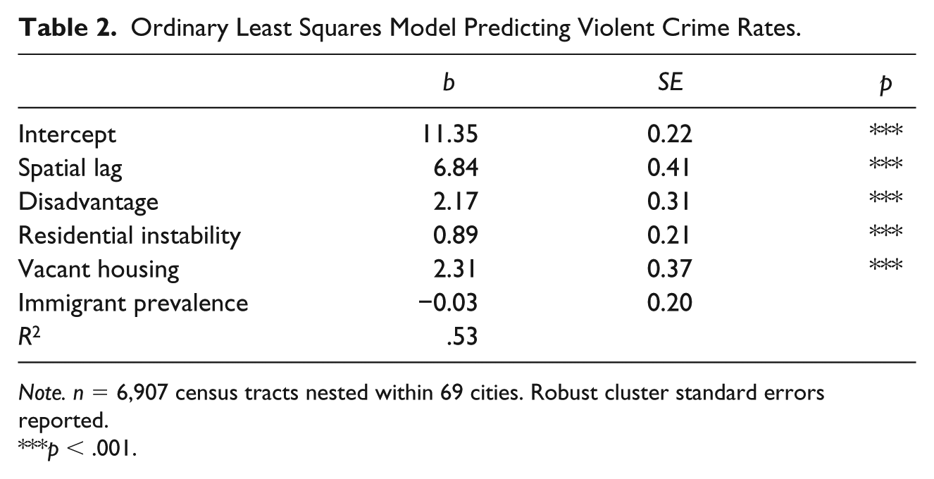
Table 2 displays the findings of OLS models to examine baseline effects of social structural predictors and spatial adjacency on local violence. Generally, the results align well with the systemic model framework. Across the entire distribution of neighborhoods, modeling reveals that vacant housing and residential instability have significant and positive effects on neighborhood violence. Not surprisingly, structural disadvantage and spatial proximity to other neighborhoods with high rates of violence are also associated with predicted increases in local violence. The effect of immigration is negative, but nonsignificant. In sum, findings point to the enduring effects of social structure and location as correlates of violent crime. But, because the OLS model represents pooled effects across the entire distribution of neighborhoods, it does not demonstrate whether certain correlates of violence vary at different segments of the distribution. In response to that limitation, quantile model results are described below.

OPEN IN VIEWER

Table 2.

Ordinary Least Squares Model Predicting Violent Crime Rates.

	b	SE	p
Intercept	11.35	0.22	***
Spatial lag	6.84	0.41	***
Disadvantage	2.17	0.31	***
Residential instability	0.89	0.21	***
Vacant housing	2.31	0.37	***
Immigrant prevalence	−0.03	0.20
R 2	.53

Note. n = 6,907 census tracts nested within 69 cities. Robust cluster standard errors reported.

***

p < .001.

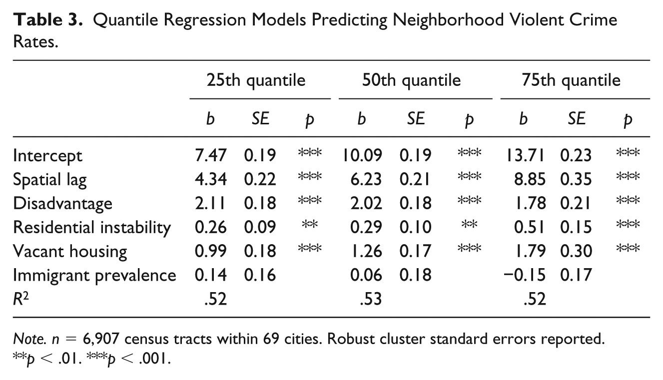
Table 3 displays quantile regression results of neighborhood violence. Contrary to what is implied by the OLS model, quantile models indicate that the effects of structural predictors depend in part on the quantile from which the distribution is analyzed. For example, at the 25th quantile, a one-unit increase in residential instability is correlated with an increase in neighborhood violent crime rates of about .26 (p < .01). Yet, the coefficient for the same predictor increases to .29 (p < .01) in the 50th quantile and .51 (p < .001) in the 75th quantile. This represents a significant change in effect size, as confirmed by equality of coefficient F tests, F(1, 6901) = 5.85, p < .05 for q25 = q75. Stated more generally, the effect of high residential turnover is most consequential in neighborhoods with moderate and high violent crime rates (located in the 50th and 75th quantiles) and least consequential in neighborhoods with the lowest crime rates (located in the 25th quantile). Also, these findings show that OLS model tends to overestimate instability effects when compared with select quantile models (OLS b = 0.89, p < .001).

OPEN IN VIEWER

Table 3.

Quantile Regression Models Predicting Neighborhood Violent Crime Rates.

	25th quantile			50th quantile			75th quantile
	b	SE	p	b	SE	p	b	SE	p
Intercept	7.47	0.19	***	10.09	0.19	***	13.71	0.23	***
Spatial lag	4.34	0.22	***	6.23	0.21	***	8.85	0.35	***
Disadvantage	2.11	0.18	***	2.02	0.18	***	1.78	0.21	***
Residential instability	0.26	0.09	**	0.29	0.10	**	0.51	0.15	***
Vacant housing	0.99	0.18	***	1.26	0.17	***	1.79	0.30	***
Immigrant prevalence	0.14	0.16		0.06	0.18		−0.15	0.17
R 2	.52			.53			.52

Note. n = 6,907 census tracts within 69 cities. Robust cluster standard errors reported.

**

p < .01. ***p < .001.

Similarly, vacant housing is a statistically significant predictor of violence across all segments of the data, but its effect also increases from the 25th (b = 0.99, p < .001) to the 75th quantiles (b = 1.79, p < .001), F(1, 6901) = 22.59, p < .001. Thus, vacant housing has its strongest effect in neighborhoods with the highest rates of violence and weakest effect in the least violent communities. And, when compared with the OLS estimate in Table 2 (b = 2.31, p < .001), linear regression overestimates vacant housing effects across all quantile models.

Immigration demonstrates a statistically insignificant effect across all model quantiles, which is in accordance with OLS model estimates. But, these results run contrary to earlier work that found immigration to be associated with significantly lower rates of violence (Martínez 2002; Martínez, Stowell, and Lee 2010). Selection effects could account for differences between Martinez and colleagues’ work and the current study.

For example, their research focused on violence in predominately immigrant communities, while this study attempts to measure an immigration effect across a broad sample of urban neighborhoods that vary according to race/ethnicity and immigrant concentration.

Models indicate that the effect of the spatial contiguity of violence increases in size as one moves from the lowest quantile of violence (25th: b = 4.34, p < .001) to the highest (75th: b = 8.85, p < .001). This finding was confirmed by equality of coefficient F tests indicating significant differences between spatial lag effects at the 25th and 75th quantiles, F(1, 6901) = 425.67, p < .001. Therefore, urban neighborhoods with the lowest rates of violence are substantially less vulnerable to the spillover effects of violence from nearby neighborhoods, compared with neighborhoods with the highest levels of violent crime.

At the same time, models reveal that the effect of structural disadvantage is opposite that of lagged violence effects across the distribution. Structural disadvantage has its greatest effect in neighborhoods with low to moderate levels of violence. A one-unit increase in disadvantage is associated with an increase of 2.11 (p < .001) and 2.02 (p < .001) in violent crime rates in the 25th and 50th quantiles, respectively. Beyond the 50th quantile, the effect of disadvantage declines continuously through the distribution of more violent neighborhoods. In fact, in the most violent neighborhoods (75th quantile), the effect of disadvantage is 15% smaller than its original size in the least violent quantile, F(1, 6901) = 6.36, p < .05. These findings illustrate that while structural disadvantage historically has been among the most resilient predictors of violence, its influence is subject to the location of a given neighborhood within the greater distribution of community violence rates.

Taken together, while most structural variables remain important correlates of violence throughout most segments of the distribution, in the more violent neighborhoods, the diminished effect of structural disadvantage is supplanted by the adjacency of violence, and to a lesser extent residential turnover, and the presence of vacant housing. Stated differently, the most violent neighborhoods are increasingly plagued by multiple social structural and locational impediments. This finding differs from effects for the least violent neighborhoods whereby the influences of adjacency, residential turnover, and vacant housing are comparatively smaller.

Supplementary Analyses

Prior studies have highlighted the importance of creating separate models for neighborhoods of various ethnoracial groups (Peterson and Krivo 2010), due to the uneven distribution of disadvantage across groups (McNulty 2001; Sampson 2009b). For this reason, ethnoracial composition predictors were excluded from models described thus far due to the statistically correlative link between race and disadvantage. To address this concern, parallel models for neighborhoods that are primarily (70% or more) non-Hispanic White or non-Hispanic Black are described below. The following points are noteworthy.

Similar to the general model discussed above, Table 4 shows that the effect of nearby neighborhood violence in predominately Black neighborhoods increases as one moves from the safest to the most violent neighborhoods (q25 b = 5.13, p < .001; q50 b = 6.50, p < .001, q75 b = 8.85, p < .001). In line with extant research, the effect of structural disadvantage on violence is race-specific. For Black neighborhoods, structural disadvantage is a significant predictor of neighborhood violence, across all quantiles (q25 b = 3.21, p < .001; q50 b = 2.53, p < .001; q75 b = 2.57, p < .01). But, contrary to the main model, the effect of structural disadvantage decreases from the 25th to 50th quantile, then levels off thereafter. This pattern indicates that disadvantage renders its strongest effects in low-violence neighborhoods, but that effect quickly tapers off for neighborhoods in the 50th and 75th quantiles. Also, contrary to the main model is that immigrant prevalence is positively associated with violence for neighborhoods located in the 50th quantile, in addition to the 25th quantile. And for Black neighborhoods, the effect of residential instability only matters for communities in the 75th quantile (b = 2.01, p < .01). In accordance with the systemic model of crime, the frequent turnover of residents could be particularly costly for the most violent neighborhoods by inhibiting the development of local ties needed for informal social control. The effect of vacant housing increases from the 25th (b = 1.26, p < .001) to the 50th quantile (b = 1.84, p < .001), but is essentially stable thereafter (q75 b = 1.82, p < .001).

OPEN IN VIEWER

Table 4.

Quantile Regression Models Predicting Violent Crime Rates in Predominately Black Neighborhoods.

	25th quantile			50th quantile			75th quantile
	b	SE	p	b	SE	p	b	SE	p
Intercept	9.11	0.78	***	12.60	0.76	***	15.30	1.29	***
Spatial lag	5.13	0.40	***	6.50	0.55	***	8.85	0.47	***
Disadvantage	3.21	0.65	***	2.53	0.73	***	2.57	0.82	**
Residential instability	−0.27	0.76		0.36	0.65		2.01	0.75	**
Vacant housing	1.26	0.26	***	1.84	0.53	***	1.82	0.44	***
Immigrant prevalence	3.04	0.87	***	2.88	1.33	*	1.12	1.75
R 2	.45			.46			.45

Note. n = 1,049 census tracts within 32 cities. Robust cluster standard errors reported.

*

p < .05. **p < .01. ***p < .001.

Model estimates for predominately White neighborhoods are shown in Table 5. The effect of disadvantage increases from the 20th (b = 1.30, p < .001) to the 50th quantile (b = 1.63. p < .001) but remains constant through the most violent neighborhoods. In fact, the change in b-weight size as indicated by the F test is only statistically significant from the 25th to the 50th quantiles. Earlier studies have found that White neighborhoods have substantially lower levels of disadvantage than communities of color and that disadvantage levels in White neighborhoods tend to cluster on the lower end of the scale. The small effect size change between the 50th and 75th quantiles on disadvantage is in line with that finding. It suggests that there is not much variation in disadvantage levels across medium- and high-violence urban White neighborhoods due to the clustering of White neighborhoods on low levels of disadvantage. And, significant immigration effects emerge across all quantiles. In accordance with the main model, the influences of nearby violence, residential instability, and vacant housing become increasingly important for understanding violence in high- versus low-violence neighborhoods.

OPEN IN VIEWER

Table 5.

Quantile Regression Models Predicting Violent Crime Rates in Predominately White Neighborhoods.

	25th quantile			50th quantile			75th quantile
	b	SE	p	b	SE	p	b	SE	p
Intercept	5.47	0.32	***	8.34	0.30	***	11.90	0.40	***
Spatial lag	2.72	0.31	***	4.42	0.32	***	6.69	0.48	***
Disadvantage	1.30	0.13	***	1.63	0.15	***	1.61	0.21	***
Residential instability	0.28	0.07	***	0.37	0.09	***	0.53	0.11	***
Vacant housing	0.26	0.19		0.56	0.14	***	1.05	0.13	***
Immigrant prevalence	0.54	0.20	**	0.93	0.25	***	1.21	0.40	**
R 2	.38			.38			.37

Note. n = 2,511 census tracts within 65 cities. Robust cluster standard errors reported.

**

p < .01. ***p < .001.

Discussion

The systemic model of social disorganization posits that social structural variables influence within- and between-neighborhood and municipal organizational networks needed to regulate local violence (Bursik and Grasmick 1993). It provides a framework for understanding how communities within the same city can vary on violent crime outcomes. But, it has limitations as a theory due to assumptions often made about its operative processes. This article addresses one key assumption—that the effects of disadvantage, residential turnover, and racial composition on localized violence are linear or consistent, regardless of where a neighborhood falls within a violent crime distribution.

Findings from this study indicate that the strength of the associations between structural elements and neighborhood violence are relative to a neighborhood’s level of violence. More specifically, as local neighborhood (tract) violence increases the statistical effect of structural disadvantage decreases—a finding that is consistent with prior research (Light and Harris 2012; McNulty 2001). I contribute, however, that while the effect of disadvantage wanes at higher levels of violence, other variables become increasingly important. Specifically, residential instability, vacant housing, and spatial location near other neighborhoods with high levels of violence demonstrate larger effect sizes for communities scoring higher versus lower in the total distribution.

Local racial composition seems to condition some of these effects. For example, the effect of residential instability matters for Black neighborhoods only when considering the 75th percentile of neighborhoods, while it matters across all segments of the data for White neighborhoods. Some research has pointed to the relative stability of predominately Black, inner-city neighborhoods, indicating that such patterns are consequential for violence (Pattillo 1998). This is not surprising, as research has testified to the limited mobility options for poor African-American residents resulting in social and economic isolation (Sharkey 2013). Findings here imply that, in predominately Black compared with White neighborhoods, the tolerance levels for violence are comparatively high partially due to relative differences in housing options. For this reason, predominately Black neighborhoods are more likely to have long-term residents for longer periods of time, until said neighborhoods reach the most extreme levels of violence within the distribution. My results show that it is in these neighborhoods whereby instability becomes problematic. On the contrary, instability proves problematic in predominately White neighborhoods across all segments of the violent crime distribution, possibly due to the mere availability of housing options afforded to Whites (Massey and Denton 1993). Although not tested here, this may undermine the regulatory capacity necessary to suppress violence in those neighborhoods, regardless of initial violence levels.

What is more, this research underlines the ways by which urban predominately Black versus White communities experience structural disadvantage-violence effects differently. Research has pointed to the concentration of disadvantage in African-American neighborhoods, as opposed to the relative lack of disadvantage in White neighborhoods (Massey and Denton 1993; Quillian 2012). Although prior research has identified a “diminishing positive” relationship between poverty and violence (Hipp and Yates 2011), the inverse statistical patterns of White versus Black neighborhood parallel models of this study highlight that the social structural production of violence is racialized. While across White neighborhoods, the effect of disadvantage increases, but levels off, in Black neighborhoods, the near opposite is true. In those communities, the effect of disadvantage decreases but levels off at the higher end of the violence distribution.

The findings from this research lend themselves to three overall public safety policy implications. First, statistical models revealed that high-violence neighborhoods are substantially more vulnerable to violent crime spillover effects than low-violence neighborhoods. Considering this finding, crime intervention approaches should simultaneously target clusters of extremely violent communities, as opposed to individual high crime neighborhoods, or risk crime reduction benefits (if any) being short-lived. Second, high-violence neighborhoods endure residential instability (and possibly outmigration) effects that are far greater than low-violence neighborhoods. This process is often coupled with extreme financial disinvestment and the shuttering of critical social institutions such as schools and banks. Assuming that this is the case, programs supporting mortgage investment in poor communities may be beneficial for the regulation of crime (Vélez, Lyons, and Boursaw 2012). Third, findings from the parallel models serve as a reminder of how the effect of structural disadvantage on neighborhood violence varies by ethnoracial composition (Peterson and Krivo 2010). Segregated Black neighborhoods are so disenfranchised that the effect of disadvantage is highest in low-violence neighborhoods—a pattern opposite that of predominately White neighborhoods. As such, policy makers and practitioners must consider how race performs as a social process by structuring the (in)availability of resources relevant to crime (e.g., job access, quality schools, banking institutions).

A few limitations are noteworthy. The statistical technique employed does not allow for the modeling of hierarchical data. Thus, models here do not speak to how broader city-level effects such as racial segregation, disadvantage, and police resources influence within-neighborhood violence. This limitation was addressed by reporting robust cluster standard errors to account for within-city correlations among census tracts. Also, the use of cross-sectional data precludes the formation of causal inferences, or consideration of shifts in violence over time. For these reasons, patterns identified here are viewed as associative or correlative in nature. Recent scholarship has advocated for community criminology scholars to shift completely to longitudinal analysis (Taylor 2015). Relatedly, concerns of endogeneity are relevant as the identified effects of social structure on violence are conditioned by violence itself. Just as social structure has demonstrated statistical association with violent crime, violent crime too could be a statistically significant predictor of social structure—a condition known as simultaneity bias. Violent crime-social structure effects have been uncovered in earlier studies (Boggess and Hipp 2010; Morenoff and Sampson 1997).

Although the National Neighborhood Crime Study data set is among the most comprehensive for the study of community-level violence, the absence of informal network measures does not allow for a full test of the systemic model. For that reason, this study is unable to consider whether the structural effects identified are mediated by private, parochial, and public order dynamics. Absent social order measures, statistical findings here can only infer social order mechanisms. Subsequent studies could consider social order dynamics in myriad ways. Proxy measures of private order could be gauged through survey items capturing not only employment status by household heads, but also the number of hours per week spent at work as an inverse measure of time spent away from children. Household heads could also be asked to report family structural attributes such as the availability of local older residents to supervise children (Anderson 1999). Similarly, parochial control could be measured through collective efficacy items, which incorporate feelings of social cohesion and a willingness of residents to intervene on behalf of the common good of the neighborhood (Sampson, Raudenbush, and Earls 1997). In addition to capturing public order mechanisms through bank loan data (Vélez, Lyons, and Boursaw 2012), research should also incorporate resident perceptions of legitimacy for municipal agencies (St. Jean 2007).

Considering the above, a strict test of social order mechanisms that accounts for the distributional properties of neighborhood violence is possible. Such a study would be realistic for neighborhoods within one city (as opposed to many), making the administration of surveys to measure social order levels more financially feasible. Examples of intracity neighborhood social science data sets used to explain crime dynamics include the Project on Human Development in Chicago Neighborhoods (Sampson 2012) and the Southeastern Pennsylvania Household Health Survey (Philadelphia Health Management Corporation 2015) among many others.

Conclusion

In this study, I have shown that understandings of the social structure–violence relationship should take into consideration the unique distributional properties of neighborhood violence. My findings build upon literature in the ecology of crime by highlighting the unstable nature of the structure-violence relationship, even within racially distinct neighborhoods. In addition, results suggest that the distributional properties of neighborhood violence within and across communities are not explainable by single statistical model solutions. Instead, a deeper understanding of neighborhood violence requires consideration of where a neighborhood is ecologically situated within the greater distribution of violence, which suggests a need to develop policy solutions that are specific and sensitive to these nuances. Considering the above findings, future research should attempt to uncover causal processes through the use of longitudinal data to analyze social structure–violence effects over time.