Formulation and Evaluation of Two Citywide Gentrification Measures

Abstract

The following exposition describes two novel empirical methods devised to measure citywide gentrification: the Dynamic Measure of Citywide Gentrification and the Cross-Sectional Measure of Citywide Gentrification. This paper tests for these measures’ viability. These measures were regressed against demographic variables, and many of the coefficients are statistically significant. These measures are associated as expected with each other when graphed and regressed, though the correlation and $R^{2}$ coefficients are lower than expected. Prominent cities identified as highly gentrified by each measure conform to expectations, and prominent cities identified as least gentrified by the Dynamic Measure also conform to expectations. For prominent cities, each measure's identification of highly gentrified cities generally conforms to the other measure. Ultimately, this paper provides evidence for the viability of these measures to assess gentrification at the level of the city. Local policymakers should expect gentrification to emerge across downtown districts.

Keywords

citywide gentrification measure urban economics

Introduction

Gentrification is among the most consequential urban phenomena of the last 60 years, provoking controversy among scholars, journalists, activists, and neighborhood denizens. On the one hand, it invites economic opportunities and improves amenities. On the other hand, it raises rents, stratifies populations socioeconomically, dilutes minority and immigrant enclaves, incites intergroup antagonisms, and some argue, displaces original residents. For good or ill, it transforms politics and physical landscapes. Understanding this monumental and contentious process requires practical research methods.

Social scientific exploration of gentrification necessitates quantitative operationalizations in addition to qualitative accounts. This paper explores two novel operationalizations of gentrification measured at the citywide level: the Dynamic Measure of Citywide Gentrification and the Cross-Sectional Measure of Citywide Gentrification. This paper provides background on gentrification, including its attributes and prevalence; describes other operationalizations that measure gentrification; explains the construction of each measure; evaluates each measure; lists descriptive statistics; interprets regressions against demographic variables; and compares these measures to assess their robustness. Finally, this paper outlines policy significance, research implications, and ideas for future research. Analyses indicate the suitability of each measure for assessing the level of citywide gentrification, which can be used in cross-city research. The present paper's primary contributions are to provide the first rigorously defended empirical methods to measure gentrification at the citywide level, and to supply corresponding data. Although previous research, not directly concerning gentrification, has examined the citywide relationship between housing prices and social change, the present measures apply accepted definitions of residential gentrification.

The Dynamic Measure divides census tracts within a central city into gentrifiable and nongentrifiable tracts at the beginning of a decade, and then some gentrifiable tracts gentrify by the decade's end. The city's gentrification score for a decade is the proportion of gentrifiable tracts that gentrify. The city's “mean” score is the average gentrification score across these decades: 1970s, 1980s, 1990s, and 2000s. For a tract to be considered gentrifiable, its median household income must fall below the median among central-city tracts, and it must contain an above-median proportion of older housing. For a tract to be considered gentrified, the proportional increase in median home value and the percentage-point increase in college-educated residents must exceed the median rate of change among central-city tracts. Additionally, the increase in median home value must surpass the rate of inflation.

The Cross-Sectional Measure assesses a city's level of gentrification by the slope of the trendline when graphing housing price versus housing age, with each census tract within a municipal boundary as a data point. The cities are then ordered from highest to lowest score, with the highest-scoring city receiving a final value of 177 and the lowest receiving a value of 1. A more detailed explanation of construction methods for each measure is later provided. Values produced by the measures may be found in the accompanying dataset (Mozell 2025).

These measures viably assess citywide gentrification. Each measure is theoretically grounded. When regressed against demographic variables, many associations are significant. The measures are statistically associated with each other. For cities with substantial citywide data, there is strong overlap between markedly gentrified cities as identified by each measure. Among cities that each measure identifies as highly gentrified, and for which substantial citywide data exist, case study and newspaper evidence substantiates that most of these cities have gentrified. Finally, cities identified as most gentrified, and which contain substantial citywide data, generally conform to anecdotal expectations. This is also true for cities that the Dynamic Measure identifies as least gentrified. As will be elaborated, cities considered to possess substantial citywide data, for the Dynamic Measure, are relatively large; and for the Cross-Sectional Measure, they have an appreciable share of older housing.

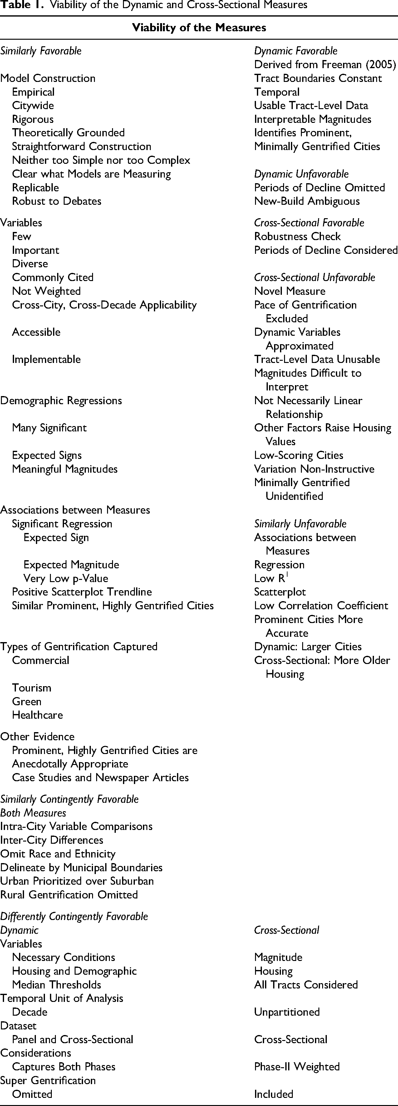
In arguing for the viability of these measures, the present paper discusses these and other considerations. Table 1 categorically outlines arguments, discussed in the present paper, addressing the viability of these measures. This table includes model characteristics that are beneficial, potentially beneficial contingent on the research question, and drawbacks.

Table 1.

Viability of the Dynamic and Cross-Sectional Measures

Viability of the Measures
Similarly Favorable	Dynamic Favorable
	Derived from Freeman (2005)
Model Construction	Tract Boundaries Constant
Empirical	Temporal
Citywide	Usable Tract-Level Data
Rigorous	Interpretable Magnitudes
Theoretically Grounded	Identifies Prominent,
Straightforward Construction	Minimally Gentrified Cities
Neither too Simple nor too Complex
Clear what Models are Measuring	Dynamic Unfavorable
Replicable	Periods of Decline Omitted
Robust to Debates	New-Build Ambiguous
Variables	Cross-Sectional Favorable
Few	Robustness Check
Important	Periods of Decline Considered
Diverse
Commonly Cited	Cross-Sectional Unfavorable
Not Weighted	Novel Measure
Cross-City, Cross-Decade Applicability	Pace of Gentrification Excluded
Accessible	Dynamic Variables Approximated
Implementable	Tract-Level Data Unusable
	Magnitudes Difficult to Interpret
Demographic Regressions	Not Necessarily Linear Relationship
Many Significant	Other Factors Raise Housing Values
Expected Signs	Low-Scoring Cities
Meaningful Magnitudes	Variation Non-Instructive
	Minimally Gentrified Unidentified
Associations between Measures
Significant Regression	Similarly Unfavorable
Expected Sign	Associations between Measures
Expected Magnitude	Regression
Very Low p-Value	Low R¹
Positive Scatterplot Trendline	Scatterplot
Similar Prominent, Highly Gentrified Cities	Low Correlation Coefficient
	Prominent Cities More Accurate
Types of Gentrification Captured	Dynamic: Larger Cities
Commercial	Cross-Sectional: More Older Housing
Tourism
Green
Healthcare
Other Evidence
Prominent, Highly Gentrified Cities are Anecdotally Appropriate
Case Studies and Newspaper Articles
Similarly Contingently Favorable
Both Measures
Intra-City Variable Comparisons
Inter-City Differences
Omit Race and Ethnicity
Delineate by Municipal Boundaries
Urban Prioritized over Suburban
Rural Gentrification Omitted
Differently Contingently Favorable
Dynamic	Cross-Sectional
Variables
Necessary Conditions	Magnitude
Housing and Demographic	Housing
Median Thresholds	All Tracts Considered
Temporal Unit of Analysis
Decade	Unpartitioned
Dataset
Panel and Cross-Sectional	Cross-Sectional
Considerations
Captures Both Phases	Phase-II Weighted
Super Gentrification
Omitted	Included

Citywide gentrification assessments may serve future academic pursuits. Cross-city analysis may systematically add more data to research questions already explored, and it also expands possible paths of inquiry. Cross-city analysis may stand alone or else supplement neighborhood-level investigation. Citywide measures can also determine differences among states and regions. These domains of study may inform prescient and inclusive city planning.

Gentrification research often compares gentrification measures against other variables. Some such variables may be best measured not at the neighborhood-level, but at the citywide level, such as political, economic, social, cultural, or physical transitions. Cross-city comparisons may contextualize urbanism, as well as geohistorical discrimination and segregation. Also, existing research has measured displacement and exclusion from neighborhoods, but little has assessed displacement and exclusion from entire cities. Community dispersal may also be compared among cities such as gentrifiers’ overtaking minority or immigrant districts and cultures. Gentrification's disequalizing effect on health and educational outcomes, as well as on access to parks and produce, may be measured citywide. Empirical measures can also supplement qualitative research (Seawright 2016).

Background and Theoretical Framework

Gentrification in Context

Shortly following the Second World War, White middle-class urban residents partook in the protracted process of suburbanization, resulting in city-suburb segregation along racial and socioeconomic lines. By diverting their consumption and tax payments from downtown districts, suburbanites enriched outlying regions at the expense of urban areas.

Suburbanization begot gradual deterioration of urban dwellings and diminishment of their property values. Inner-city public investment also declined as tax revenues fell. Beginning en force in the 1970s, White, affluent, suburban residents entered the city, forming new sociopolitical constituencies. These residents redeveloped formerly neglected areas, thus raising housing prices and encumbering the present inhabitants. This latter process, of reclaiming the city, is broadly known as gentrification.

Newcomers were most often young, White, better educated, and relatively high earning (Couture and Handbury 2023). Original residents were more likely to be poor, less educated, and identifying as a minority. This transformation often disrupted whole communities, leading to social fragmentation and cultural displacement (Croff, Hedmann and Barnes 2021). Many observers find gentrification to be widespread (Richardson, Mitchell and Edlebi 2020; Robiou 2018).

Gentrification Debates

A foundational debate concerns whether gentrification has been driven by capital and the state or else gentrifier demand for urban housing and occupational restructuring. Harvey (1982) argued the former explanation, capitalists responding to an overaccumulation crisis by investing in devalued cities. The state provides physical and social infrastructure to facilitate urban development and profitability. Capital and the state thereby reshape urban landscapes, instrumentalizing gentrification and displacement. Smith (1979) forwarded rent gap theory, real estate developers investing when urban potential rents sufficiently exceed ground rents, spurring gentrification. Conversely, other scholars argued that the occupational transition to white-collar services, the baby boom, and gentrifier taste for metropolitan living have induced gentrification (Berry 1985; Ley 1986). Real estate firms and financiers are often essential but respond to demand. Theorists who forward these latter explanations generally affirm the importance of public policy.

Gentrification is shaped by context. According to Harvey (1982), gentrification is induced most dramatically in cities that were previously devalued, that capital networks identify as investment opportunities, and that are administrated by governments effectively enabling capital. Berry (1985) described heavily gentrifying cities as those that are prominent, marked by a strong white-collar service sector, and attractive to potential gentrifiers.

Researchers forwarding capital-led gentrification generally agree finance is critical in reconfiguring urban space (Harvey 1982). However, Aalbers (2019) argued that, post-2008, global finance (in conjunction with the state) has played an amplified role, terming this period “fifth-wave gentrification.”

The literature debates the transposability of the term gentrification. Lees, Shin and López-Morales (2016) observed that global finance has sought investment opportunities in developing countries, initiating gentrification there. However, Ghertner (2015) argued that many instances of displacement in the global South differ in process and severity from Euro-American dislocation, and so the term may be misapplied. In developing countries, real estate capital may harness “extra-economic” forces, pressuring governments to dislodge residents from common or publicly owned land, inducing starker displacement and representing harsher state violence.

Some scholars have argued that gentrification inducing displacement is overstated (Easton et al. 2020; Freeman 2005; Freeman and Braconi 2004; Hamnett 2003). This contradicts other evaluations (Elliott-Cooper, Hubbard and Lees 2020; Marcuse 1986; Slater 2006). Many journalists, activists, and original residents have cited displacement as a problem.

Analysts have contested whether, independently of displacement, gentrification helps or harms original residents. Curran (2007) demonstrated gentrification displacing industry. However, Freeman and Braconi (2004) noted gentrification invites retail investment, improved public services, and employment opportunities. Ellen and O’Regan (2011) found original residents enjoy differential income gains, and that they report greater increases in neighborhood satisfaction than identified in other low-income neighborhoods.

A related contention concerns whether gentrification engenders social mixing or promotes segregation. Some research (Ellen and O’Regan 2011; Freeman and Braconi 2004) has found evidence of social mixing, while other assessments (Lees 2008; Slater, Curran and Lees 2004) have observed geographical or relational segregation.

Observers disagree on the appropriate response to gentrification. Marcuse (1985) urged mitigation, advising proactive zoning and other strategies. Alternatively, some radical scholars demanded a right to the city. Lefebvre (1968), who influenced gentrification debates, characterized capitalism as having commodified urban space to serve property owners. Thus all urban inhabitants must collectively appropriate the space and reshape it to serve the public, which would include fostering enjoyment and social integration.

The two measures likely function regardless of gentrification's impetus; reasons for inter-city differences; the role of finance; whether the term can always be applied to developing countries; its effect on original residents including displacement, social mixing, and other outcomes; and the appropriate response. For the Dynamic Measure, none of these precludes shifting demographics and housing characteristics in the United States, and for the Cross-Sectional Measure, older housing's price appreciation.

Neighborhood vs. Citywide Phenomenon?

Most scholars conceptualize gentrification at the neighborhood level. However, both the Dynamic and Cross-Sectional Measures conceptualize gentrification as occurring across densely populated urban districts, thereby acquiring a citywide character. The Dynamic Measure confines gentrification to the central city while the Cross-Sectional Measure assumes gentrification occurs primarily in older neighborhoods, which tend to reside in urban districts. These assumptions suppose urban centers often gentrify holistically. However, intracity gentrification may begin as localized phenomena, and parts of a gentrifying city center may be excluded from gentrification or even face deterioration. Citywide gentrification measures are lacking relative to neighborhood-level measures, and so new assessment methods would aid potential research.

Comparing Operationalizations of Gentrification

Other quantitative gentrification operationalizations are here described. Preis et al. (2021) cited methods measuring gentrification devised for four cities: Los Angeles, Philadelphia, Seattle, and Portland, Oregon. The authors applied these measures to Boston. A finding was that the gentrification-assessment method greatly affected which neighborhoods were found to be gentrifying. The Los Angeles method was constructed by the Los Angeles Innovation Team and Pudlin (2016, 2018); Philadelphia by Ding, Hwang and Divringi (2016); Seattle by the Seattle Office of Planning & Community Development (2016); and Portland by Bates (2013).

Los Angeles, Seattle, and Portland used variables capturing characteristics of individuals, households, and neighborhoods. These measures likely would not suit large-scale, cross-city research. First, some variables require in-depth knowledge of a city that may be difficult to apply across many cities. For instance, Seattle measured distance to transit busses, jobs, attractive business, civic infrastructure, and developmental properties. Second, some variables may have different implications depending on the city. In this regard, Seattle, Los Angeles, and Portland all used race-based measures, and Seattle used share of non-English speakers. Third, these models used many variables, which may fit a particular city, but might clutter a cross-city model.

Among the four cities’ models, the Philadelphia method is most suitable for cross-city research. Using housing and demographic data, the Philadelphia measure initially divided cities into gentrifiable and nongentrifiable census tracts, and then at the end of a period some gentrifiable tracts have gentrified. At a decade's outset, gentrifiable tracts were those with median household income below the city median. For a gentrifiable tract to have gentrified, the share of college-educated residents must have increased above the citywide median rate; and either median rent or median home value must have appreciated above the citywide median rate. For the present paper, the Philadelphia method was not selected to be expanded to a citywide measure because, foremost, it does not contain a direct indication of neighborhood disinvestment.

Other neighborhood gentrification models have been designed. Bostic and Martin’s (2003) model (based on Hammel and Wyly’s (1996) model) used tract-level demographic data for the 50 largest metropolitan areas to measure gentrification, in part drawing upon nine indicators. Walks and Maaranen (2008) constructed a model using tract-level demographic and housing variables. Ellen and O’Regan (2011) relied on a census tracts’ average household income to specify low-income neighborhoods, and increase in income to determine neighborhood change. Desmond and Gershenson (2017) formulated a model similar to Freeman’s (2005) for Milwaukee (Freeman to be discussed).

Other authors used novel means to measure gentrification. For instance, Barton (2014) identified gentrification in New York City by examining New York Times articles. Hwang and Sampson (2014) used Google Street View to assess neighborhood reinvestment. Papachristos et al. (2011) in part counted coffee shops in an area. Kreager, Lyons and Hays (2011) in part assessed the level of neighborhood mortgage lending. Holm and Schulz (2018) constructed GentriMap, a tool measuring gentrification using housing and demographic data. While conducting a meta-analysis of Philadelphia from 1970 to 1980, Galster and Peacock (1986) found that the mix of selected variables influenced whether a neighborhood was deemed to have gentrified.

For the present research, none of these measures was extrapolated for citywide models. In service of generalizability, variables that differ in importance among cities are not appropriate. Measures devised for a specific city, such as New York City, may not apply evenly across cities. To maintain rigor, the Dynamic and Cross-Sectional Measures limit the number of variables to four and two, respectively. Many definitions of gentrification include these variables, which capture important elements of gentrification.

Including many variables in a model might increase the likelihood of misclassifying a city. For instance, if the value of a single variable alone can identify the presence or absence of gentrification, the model risks volatility. Additionally, if multiple such variables are included, it may be unclear exactly what the model's outcome indicates. If many variables must align, the model risks rigidity. A weighted scoring model risks diminished rigor. Furthermore, it may be prudent to exclude variables highly correlated with others. Different research intentions merit different methods, and the models devised for the present paper are designed for large-scale, cross-city analysis.

Some researchers intended to assess gentrification in particular neighborhoods, compare neighborhoods in a single city, or analyze particular kinds of neighborhoods or cities. These measures may employ less commonly used variables and enjoy more granular analysis, but may also sacrifice generalizability across cities. Measures with more variables may be less rigorous, but they may more completely capture specific dynamics of particular neighborhoods or cities.

The present discussion assesses the above neighborhood models’ capacity to construct a citywide measure. Holm and Schulz’s (2018) measure may, if expanded, compare gentrification levels across cities. However, the authors used many weighted variables to measure gentrification, which may weaken rigor. Ellen and O’Regan (2011) used tract-level median household income, which could be expanded to citywide analysis, but the authors did not use housing-related variables directly in the measure. Ellen and O’Regan, thus, omitted important elements of gentrification including a measure of neighborhood disinvestment.

The following models would likely be less suited to expansion. Bostic and Martin (2003) and Hammel and Wyly (1996) used many variables, some of which were likely highly correlated. In defining tracts eligible for gentrification, Galster and Peacock (1986) used variable thresholds that may not all be appropriate among many cities and periods. Walks and Maaranen (2008) considered percentage of artists as well as percentage of professionals and managers, which capture two phases of gentrification. However, if one phase principally transpires at a time, then incorporating one variable diminishes the impact of the other.

Barton’s (2014) analysis likely underperforms beyond New York City. If applied across cities, Hwang and Sampson’s (2014) model would require substantial investment and might suffer from inconsistency. Regarding the model devised by Papachristos et al. (2011), the number of coffee shops in an area likely differs across cities because land value and coffee consumption also markedly differ. Additionally, the number of coffee shops has not commonly been cited as integral to gentrification. Regarding Kreager, Lyons and Hays’ (2011) model, mortgage lending has not directly been included in most definitions of gentrification. However, all of these models innovatively and constructively assess gentrification for particular contexts.

Comparing the Measures to Other Forms of Gentrification

Various authors have expanded definitions of gentrification, to which the two measures are here compared. Although the following characterizations productively reframe gentrification, a measure's construction prioritizes particular descriptions. The two measures are intended to assess foundational definitions of residential gentrification.

Rural gentrification entails “affluent households migrating to the countryside” (Smith and Phillips 2001). Neither the Dynamic nor the Cross-Sectional Measure captures rural gentrification because they confine analysis to municipal boundaries. Also, census tracts standardize population, not area, so rural locations may comprise too few tracts for adequate assessment. Many researchers have defined gentrification as urban, and so excluding rural areas may be prudent.

In addition to urban areas, some authors have described suburbs as loci of gentrification (Hudalah and Adharina 2019). Both measures delineate a city's geography by its municipal, not metropolitan, boundary. Also, the measures define a potentially gentrifying tract as containing relatively older housing. Thus they best identify gentrification in urban areas. If a research question focuses on suburban localities, the Dynamic Measure would likely perform better than the Cross-Sectional Measure because the latter presupposes a downtown core.

Super-gentrification entails upgrading already-gentrified neighborhoods (Lees 2003). Because the Dynamic Measure defines gentrifiable neighborhoods as below-median income, it excludes this process. By comparing price differences among all properties, the Cross-Sectional Measure emphasizes super-gentrification.

New-build gentrification entails “developments … often built on brownfield sites or on vacant and/or abandoned land; as such they do not displace a preexisting residential population in the same way as classical gentrification has done” (Davidson and Lees 2005). The Dynamic Measure ambiguously relates to new-build gentrification. This measure likely captures it if it occurs within disadvantaged neighborhoods because, although this process adds to the housing stock, it entails “capital reinvestment, social upgrading, and middle-class colonization” (Davidson and Lees 2005). However, the Dynamic Measure likely discounts new-build gentrification when it occurs in relatively affluent neighborhoods. New-build gentrification entails constructing luxury units, complicating the Cross-Sectional Measure's assumption that newer housing is less expensive in gentrifying cities.

Commercial gentrification, which includes retail gentrification, involves higher-value businesses replacing lower-value ones (Zukin et al. 2009). Tourism gentrification is “the transformation of a middle-class neighbourhood into a relatively affluent and exclusive enclave marked by a proliferation of corporate entertainment and tourism venues” (Gotham 2005). Green gentrification entails a city constructing or rehabilitating green spaces, attracting affluent in-movers (Quinton, Nesbitt and Sax 2022). Healthcare gentrification entails gentrification's reorganizing local healthcare, compositionally and geographically, favoring wealthy residents and disadvantaging vulnerable denizens (Cole et al. 2021).

Commercial gentrification in part transpires in mixed-use neighborhoods alongside residential gentrification. Both measures likely capture commercial gentrification when it occurs this way. Likewise, in areas where tourism gentrification, green gentrification, and healthcare gentrification develop, residential gentrification also likely transpires, and so the Dynamic and Cross-Sectional Measures are likely to capture these types of gentrification when they emerge. However, strong gentrification scores (which measure residential gentrification) do not strictly imply these four gentrification varieties.

Constructing the Dynamic Measure of Citywide Gentrification

As outlined, gentrification raises values of property previously suffering from disinvestment, invites new residents, and potentially displaces original residents. Gentrification is an urban and neighborhood phenomenon, and not a state of being but a process. Additionally, many neighborhoods within an urban center may gentrify together.

The Dynamic Measure, a method similar to Lance Freeman's (2005) measure, was constructed to calculate gentrification for the present study. The Dynamic Measure also methodologically resembles Maciag’s (2015) measure, which, like the Dynamic Measure, assessed gentrification at the citywide level. Freeman's measure has often been cited in academic research (Easton et al. 2020; McKinnish, Walsh and White 2010; Preis et al. 2021).

As part of the author's research, Freeman attempted to determine which neighborhoods had gentrified over a decade. The author assessed neighborhoods at a decade's beginning and end. At the beginning, the author designated neighborhoods as “gentrifiable” or “nongentrifiable.” At the end, gentrifiable neighborhoods may have gentrified.

Freeman identified gentrifiable neighborhoods as those within the central city; whose residents have median household income below the metropolitan area median; and (to measure disinvestment) with proportion housing built within the last 20 years below median for the metropolitan area. By the decade's end, gentrifying neighborhoods will have experienced an increased percentage of residents 25 and older with at least a four-year college degree, greater than the median percentage increase for the metropolitan area; as well as increased real housing prices.

The Dynamic Measure assesses gentrification for the 1970s, 1980s, 1990s, and 2000s. It also averages the four decades’ gentrification scores, here termed the mean measure of gentrification. The former evaluation produces a panel dataset, while the latter evaluation produces a cross-sectional dataset.

For the Dynamic Measure, the unit of intracity analysis is the census tract, and the unit of intercity analysis is the city. Included census tracts are found within the central city, determined by the 2010 Census. Included cities were drawn from a 187-city sample devised for other research. Due to methodological constraints, only 161 cities could be scored by the Dynamic Measure. All 50 of the largest U.S. cities are contained in the 161-city sample.

To construct the Dynamic Measure, the central city limits were divided into 2010 census tracts. Census tracts represent urban neighborhoods. As in Freeman's measure, at a decade's outset, each tract was determined to be “gentrifiable” or “nongentrifiable,” and at a decade's conclusion, gentrifiable tracts were determined either as “gentrified” or “not gentrified.” Gentrifiable tracts are those with a median household income below the central-city median among census tracts, and they contain an above-median proportion of older housing.

For a tract to be considered gentrified, its proportional increase in median home value, and the percentage-point increase in residents aged 25 or older with at least a four-year college degree, must exceed the median rate of change among central-city tracts. Additionally, the proportional increase in median home value must surpass the rate of inflation. Given how gentrification is here defined, nongentrifiable tracts did not gentrify even if they met these criteria. A city's gentrification score for a decade is the proportion of gentrifiable tracts that had gentrified over that decade; or, for the mean measure of gentrification, each decade's gentrification score averaged.

In order to compare census tracts across decades, “crosswalk data” were employed via the Integrated Spatio-Temporal Aggregate Data Series (ISTADS) (Minnesota Population Center n.d.), which holds the geographical area of 2010 census tracts constant from 1970 through 2010 irrespective of how the Census delineated these tracts in previous decades. All tract-level data were derived from this dataset. Census tract boundaries often change from decade to decade, and so holding boundaries constant reduces variance in the model.

Differences between the Dynamic Measure and Freeman's measure are these: Freeman's measure assesses gentrification at the neighborhood level while the Dynamic Measure assesses it for cities; Freeman's compares variables within the metropolitan area, while the Dynamic Measure compares variables within the central city; Freeman's stipulates that real home value must have increased, while the Dynamic Measure includes this stipulation, along with the requirement that a tract's median home value increase proportionally faster than the median proportional increase among central-city tracts; and Freeman's stipulates older housing as that which was constructed before the past 20 years instead of, due to data constraints, 30 years by the Dynamic Measure. Freeman's supplements those variables that use “median” with variables that use the “40th percentile.” Research not included in this paper indicated that the median and 40th percentile methods yield similar results, and so for simplicity the 40th percentile method was not included herein. However, the accompanying dataset (Mozell 2025) does include 40th percentile figures.

Analysis of the Dynamic Measure of Citywide Gentrification

An advantage of the Dynamic Measure is that prevailing scholarly definitions helped inform Freeman's variables (Freeman 2005). These definitions variously cited particular components of gentrification: lower-income residents initially occupying neighborhoods; a proportional increase in relatively affluent residents; inner-city reconstruction; and rising housing values. Freeman's measure and the Dynamic Measure include these considerations.

The Dynamic Measure bears several other conceptual advantages. First, it is rigorous, only four variables included. These variables are drawn from Census data, are commonly used, and are likely relevant across cities. The variables are not weighted and represent distinct phenomena, meriting concurrent inclusion. Second, the model uses temporal data, allowing researchers to trace gentrification over time. Third, the model can compile usable tract-level data. Fourth, the model's simplicity eases compilation and implementation.

Fifth, using college-degree holders is useful. While income may fluctuate macroeconomically, and home values with housing markets, a large increase in educated residents likely indicates new residents. Additionally, using education captures the influx of “artists and professionals who have relatively low incomes” (Freeman 2005), new residents who “often pioneer gentrification.”

Sixth, this measure defines gentrifiable neighborhoods as initially low income. Otherwise, this measure could include high-income neighborhoods, which is not commonly perceived as appropriate. Seventh, older housing indicates private and public disinvestment. A substantial share of older housing creates the opportunity for gentrifier and local government reinvestment. Additionally, using housing age likely emphasizes urban areas over suburban areas. Eighth, this model cites gentrifying neighborhoods as experiencing dramatically increased housing values, conforming to most qualitative conceptions.

Ninth, at least three academic case studies or reports investigating gentrification have centered on 12 of the 14 most gentrified large cities (see Figure A1 in the appendix). Additionally, at least two newspaper articles have indicated gentrification to have developed there. Exceptions in both cases are Colorado Springs and Albuquerque. A reference list including these case studies, reports, and newspaper articles can be found in the present paper's corresponding dataset (Mozell 2025).

As for potential disadvantages, first, the Dynamic Measure is more precise for larger cities with more census tracts, but smaller cities on aggregate likely yield meaningful results. Second, the Dynamic Measure compares tracts to their central city limits rather than to the entire U.S. Some tracts considered less affluent nationally may be, for a given city, considered affluent enough to be nongentrifiable, and vice versa. Constructing a measure comparing variables not within cities, but nationally, may benefit future research. Such analysis would standardize specific values among cities. It would also limit gentrifiable neighborhoods in cities having previously undergone extensive gentrification. Gentrification may be more transformative, both demographically and institutionally, in formerly impoverished cities.

However, intercity comparisons would expand the share of gentrifiable tracts in lower-income, more disinvested cities, and restrict these tracts in more affluent cities with newer housing. Using intracity comparisons roughly standardizes the share of gentrifiable tracts across cities, easing conceptualization. Also, gentrification is often considered a city-centric development, both in processes and outcomes.

The third disadvantage is that median variable thresholds preclude gentrification transpiring across a majority of tracts. Given extensive citywide gentrification, some anecdotally observed gentrifying tracts may thereby be excluded from consideration. However, limiting gentrification to certain tracts may benefit the model because gentrification usually affects only particular neighborhoods at particular times.

Fourth, only central-city tracts are considered, and the variable, older housing, is included. Therefore many suburban census tracts may not be identified as gentrifiable. However, this may also be advantageous because gentrification chiefly unfolds in downtown districts. Also, many scholars have defined gentrification as an urban phenomenon. Ultimately, the Dynamic Measure emphasizes rigor and cross-city applicability. The disadvantages were weighted against corresponding advantages.

Dynamic Measure of Citywide Gentrification – Descriptive Statistics

Table 2 lists descriptive statistics of the Dynamic Measure. A minority of total tracts were gentrifiable, and among them a minority have gentrified. Statistics for the model's underlying variables conform to general expectations.

Table 2.

Dynamic Measure of Citywide Gentrification.

Total Tracts	60,142
Gentrifiable	19,257
Percentage of Total	32.0%
Gentrified	5150
Percentage of Gentrifiable	26.7%
Percentage Older
Gentrifiable Tracts
Mean	66.3%
Median	32.5%
All Tracts
Mean	49.9%
Median	11.2%
MHHI
Gentrifiable Tracts
Mean	$17,016
Median	$7,699
All Tracts
Mean	$25,259
Median	$9,522
Percentage Change in Educated
Gentrified Tracts
Mean	10.9%
Median	8.5%
All Tracts
Mean	4.4%
Median	4.4%
Percentage Change in Real Housing Price
Gentrified Tracts
Mean	112.9%
Median	53.3%
All Tracts
Mean	68.7%
Median	47.7%

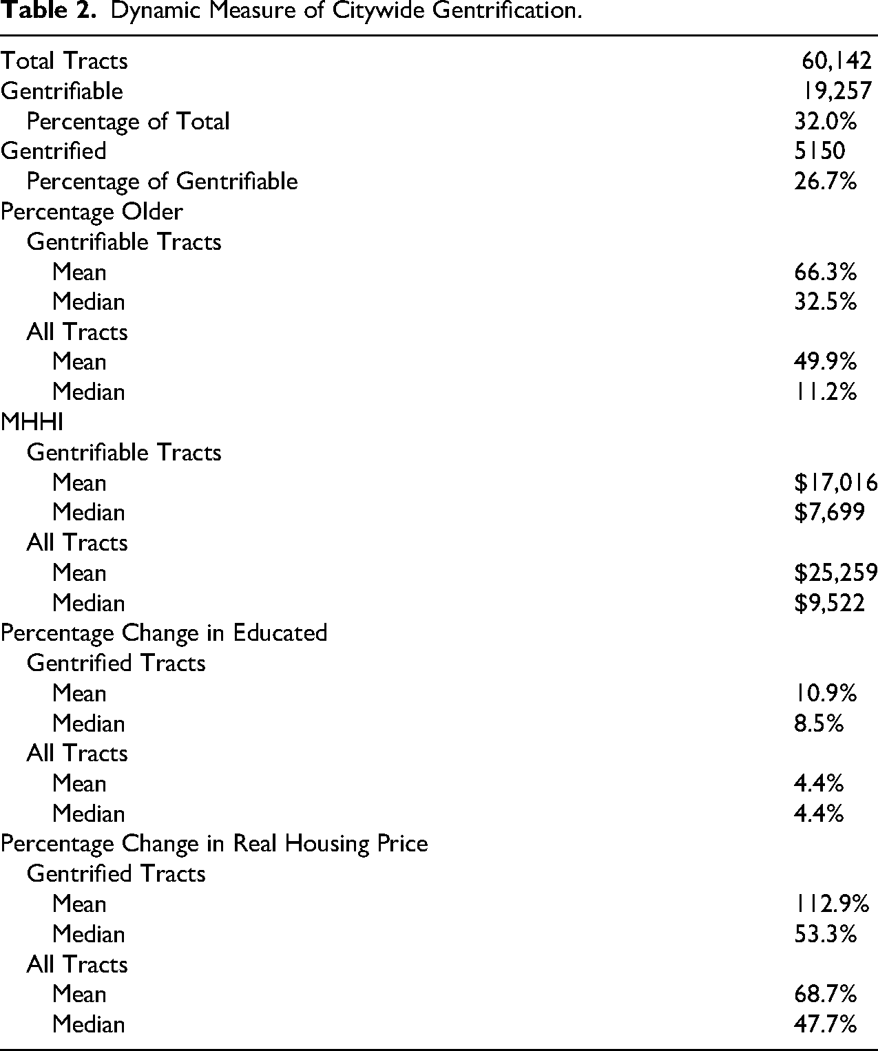
Figure A1 in the appendix indicates the Dynamic Measure's gentrification scores. Cities that had a 2010 population greater than 400,000 are highlighted. Most larger cities in the top quartile conform to anecdotal expectations: Austin, TX, Raleigh, NC, Portland, OR, Colorado Springs, CO, Charlotte, NC, Denver, CO, Nashville, TN, San Francisco, CA, Washington, D.C., Seattle, WA, Atlanta, GA, Sacramento, CA, Chicago, IL, and Albuquerque, NM. Among larger cities in the bottom quartile, Detroit had experienced significant disinvestment between 1970 and 2010. Many parts of Long Beach, Miami, and Honolulu were affluent before 1970. Fresno has gentrified markedly since the 2000s, but from the mid-1960s until the 2000s, it had experienced dramatic economic decline and White flight (Yung et al. n.d.). Gentrification in Los Angles has occurred later and less intensely than in many other cities (Toplansky, López del Río and Murphy 2019).

Regressing the Dynamic Measure against Demographic Variables

The Dynamic Measure was regressed against 10 demographic variables from the 2010 American Community Survey, as expressed in Table 3 (U.S. Census Bureau 2010a, 2010b, 2010c, 2010d, 2010e, 2010f, 2020). For this research, two sets of regressions were run, the first regressing variables separately and the second regressing them together. Independent variables are these: population density (a measure of urbanization); median household income; proportion poverty; proportion White; proportion foreign born; proportion female; median age; proportion renter; average household size; and proportion with minor. Proportion poverty is intended to assess early-stage gentrification, while median household income is intended to evaluate late-stage gentrification. Including two affluence measures also acts as a robustness check. Proportion college educated was not included because education is integral to the construction of the Dynamic Measure, and so it likely would not yield interesting results. As will be discussed, the Cross-Sectional Measure was regressed against it.

Table 3.

Dynamic Measure Regressed against Demographic Variables.

	Regressed Separately	Regressed Together
Population Density	0.00174	−0.00315
(1000 People per Sq. Mile)	0.00261	0.00338
$N$	158
$R^{2}$	0.0028
MHHI	0.00334***	0.00230*
($1000s; 2010 Dollars)	0.000758	0.00138
$N$	161
$R^{2}$	0.11
Proportion Poverty	−0.380***	−0.579**
	0.116	0.247
$N$	161
$R^{2}$	0.063
Proportion White	0.0307	−0.206***
(Not Hispanic or Latino)	0.0413	0.0628
$N$	161
$R^{2}$	0.0035
Proportion Foreign Born	0.123	0.0482
	0.0978	0.162
$N$	161
$R^{2}$	0.0098
Proportion Female	−1.067*	0.115
	0.576	0.644
$N$	161
$R^{2}$	0.021
Median Age	0.00118	−0.00581**
	0.00182	0.00252
$N$	161
$R^{2}$	0.0026
Proportion Renter	−0.00767	−0.0214
(Housing Units)	0.0896	0.157
$N$	161
$R^{2}$	0.00
AHHS	−0.0672*	−0.0277
	0.0367	0.0825
$N$	161
$R^{2}$	0.021
Proportion with Minor	−0.447***	−0.860***
(Households)	0.142	0.268
$N$	161	158
$R^{2}$	0.059	0.26

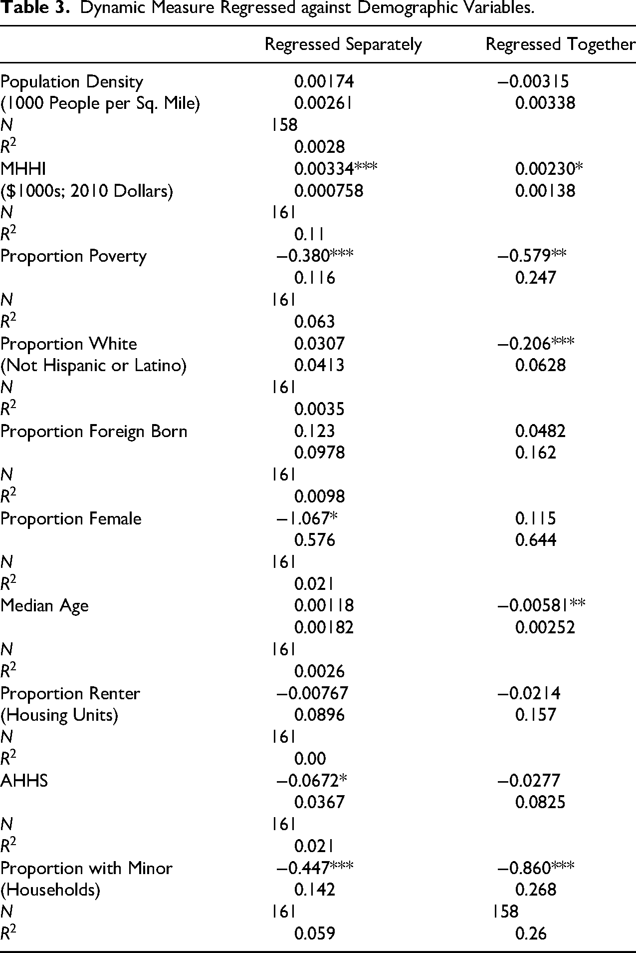
Contrary to the hypothesis that population density would be significant and positive, this variable is insignificant in both sets of regressions. On the one hand, this result makes sense because, in cities without an older downtown core, the model's mechanics allow measuring suburban transitions. On the other hand, this result is puzzling because highly urban cities are generally considered to experience more dramatic gentrification than highly suburban cities. The insignificance of population density is a potential benefit because this result may indicate that the Dynamic Measure can be used in both high- and low-density cities, as well as in largely suburban cities. This result indicates a potential drawback if a researcher defines gentrification fundamentally as an urban phenomenon.

Conforming to hypothesis, median household income and proportion poverty are significant in both sets of regressions, of the expected sign, and within expected ranges of magnitude. Contrary to hypothesis, proportion White is significant and negative in the multiple regression. This might lend some credence to findings in other research that gentrification does not dramatically displace original residents (as discussed). This finding might also diverge from other research that gentrification has historically been more likely to occur in majority White neighborhoods than majority Black neighborhoods (Rucks-Ahidiana 2021). It was hypothesized that proportion foreign born would be negative, but it is insignificant in both sets of regressions.

No hypothesis was made for proportion female, and this variable is significant and negative in the simple regression. Conforming to hypothesis, median age is significant and negative in the multiple regression, suggesting that gentrifiers tend to be relatively young. Modeling it concurrently with proportion with minor may render it significant in the multiple regression. Because gentrifiers are relatively wealthy, they may be more likely to own residences. However, because they are disproportionally urbanites, they may be more likely to rent. Thus no hypothesis was made for proportion renter, which is insignificant in both sets of regressions. Conforming to hypothesis, average household size is significant and negative in the simple regression. Conforming to hypothesis, proportion with minor is significant and negative in both sets of regressions, suggesting that gentrifiers choose to have smaller families. Average household size's insignificance in the multiple regression, when modeled concurrently with proportion with minor, may suggest that gentrifiers’ choice to have fewer children outweighs gentrifiers’ choice to remain single or live in single-family units.

Constructing the Cross-Sectional Measure of Citywide Gentrification

The Cross-Sectional Measure is predicated on older housing increasing in value in gentrifying urban centers due to gentrifier demand for refurbished older housing. This demand may be driven by a desire to occupy trendy older units or because demolishing existing older units is expensive or illegal. Like Freeman's measure, older housing also represents disinvestment in pregentrified neighborhoods. During gentrification, suburb-to-city migration depresses suburban housing prices relative to older, urban housing. Older housing's price appreciation might, then, displace former residents. In ungentrified cities, migration to the urban center from the suburbs did not occur as intensely, and so the suburb-to-downtown housing price ratio is greater than in highly gentrified cities.

The Cross-Sectional Measure was devised for a 177-city sample (154 of which overlap between the two measures). Like the Dynamic Measure, data constraints precluded including some cities among the 187-city sample. For the Cross-Sectional Measure, each city's municipal boundary was divided into census tracts. Urban housing, and some suburban housing, were likely captured in this designation. Using data from the 2010 Census, for each census tract, the percentage of older housing and the median home value were identified. The percentage of older housing was determined by the percentage of units constructed before 1940.

Each city was graphed, each census tract as a data point. For each tract, the dependent variable is median home value, and the independent variable is percentage of older housing. The slope of the trendline through all of a city's census tracts is the “raw score” of gentrification. These data were so analyzed using SimplyAnalytics software (SimplyAnalytics 2003) drawing upon data from the 2010 Census. The year 2010 was selected to match the mean method employed by the Dynamic Measure, better allowing comparisons between the two models.

Older housing tends to disproportionately exist within the inner city, and so if older housing is relatively more expensive than newer housing, the trendline's slope tends to be steeper. A steeper trendline likely indicates that affluent gentrifiers have moved into the downtown area, thereby increasing the value of inner-city, older housing and depressing the value of suburban, newer housing.

The raw score suffers from outliers because a trendline slope may approach infinity or negative infinity. To solve this, cities were ordered from greatest to least, with the city identified as most gentrified receiving a score of 177 and the city identified as least gentrified receiving a score of 1. The Cross-Sectional Measure, therefore, quantifies gentrification not by the raw scores, but by the order of raw scores. Cities with a larger proportion of older housing are more reliable estimates as their data spans a greater range along the graph's x-axis.

Other outlier mitigation strategies were tested. These included quantifying raw scores by their logarithmic value, measuring the trendline in radians, and removing outliers from the dataset. External analysis indicated the order method to be optimal.

Analysis of the Cross-Sectional Measure of Citywide Gentrification

The Cross-Sectional Measure is cross-sectional because it does not directly include variables that change over time. The Dynamic Measure traces a process. In using a city's array of census tracts for the year 2010, the Cross-Sectional Measure depicts geographical structure. Because gentrification is a dynamic process, it might be argued that temporal information is necessary to determine the presence and level of gentrification, rendering the Cross-Sectional measure infeasible.

Although this model uses cross-sectional data, it is meant to capture changes in urban neighborhoods over a city's history. The key is that inner-city housing tends to be older than suburban housing. In gentrifying cities, wealthy residents have entered the inner city, creating demand for refurbished older housing that had previously deteriorated. The older, refurbished housing price has then risen. Simultaneously, a city's newer suburban housing, from which many gentrifiers likely emerged, was depressed in value as gentrifiers sold their previous residences. As a city gentrifies, suburban housing prices may still rise, but likely not at the same rate as urban housing. If newer, suburban housing is expensive relative to inner-city housing, then extensive gentrification is less likely to have occurred.

The model's first benefit is its rigor. Theory informs the model. Only two variables are used, which are drawn from the 2010 Census and commonly employed. Using fewer variables also indicates the model's exact process. The included variables are likely relevant across cities, allowing cross-city research. Finally, the model's simplicity streamlines implementation.

Second, the model can serve as a robustness check, especially alongside the Dynamic Measure. Third, the Dynamic Measure's decade-level distinctions are arbitrary though necessary if using ISTADS data and if choosing standard periods. The Cross-Sectional Measure evaluates citywide development continuously. Fourth, by using variable medians, the Dynamic Measure necessarily restricts the number of gentrifiable and gentrifying tracts, which may exclude some gentrifying neighborhoods in expansively developing cities. The Cross-Sectional Measure considers all older tracts. Fifth, the Dynamic Measure's minimum score is zero. During a given decade, cities that remained stagnant receive similar scores as cities that experienced disinvestment. The Cross-Sectional Measure reflects periods of decline.

Sixth, the top 25 cities with at least 10 percent older housing generally conform to expectations (see Figure A2 in the appendix): Berkeley, CA, Charleston, SC, Washington, D.C., San Francisco, CA, Newport, RI, Seattle, WA, Providence, RI, New York City, NY, Savannah, GA, Evanston, IL, Santa Barbara, CA, Boston, MA, Atlanta, GA, Asheville, NC, Columbia, SC, Olympia, WA, New Orleans, LA, Denver, CO, Santa Cruz, CA, Portland, OR, Richmond, VA, Norfolk, VA, Portland, ME, Montpelier, VT, and Augusta, ME. Seventh, at least three academic case studies or reports investigating gentrification have centered on each of 18 of these 25 cities, and at least one case study or report has centered on an additional four. Exceptions are Evanston, Montpelier, and Augusta, ME, though Evanston is mentioned in case studies on Chicago. At least two newspaper articles have indicated gentrification having developed in 24 of these cities, the exception being Montpelier. A reference list including these case studies, reports, and newspaper articles can be found in this paper's corresponding dataset (Mozell 2025).

The following advantages may favor particular types of analysis. First, only housing variables are included, which may benefit housing-focused research. Second, by using education, the Dynamic Measure assesses phase-I and phase-II gentrification comparably (artists and professionals are similarly educated). By using housing price as the primary measure of gentrification, the Cross-Sectional Measure weights phase-II gentrification more heavily than phase-I gentrification (professionals have greater purchasing power than artists). Third, the Cross-Sectional Measure captures gentrification in older, largely urban areas; the Dynamic Measure may capture suburban transitions if suburban areas begin a decade relatively old and low income compared to central city tracts. A researcher defining gentrification as an urban process may, therefore, favor the Cross-Sectional Measure.

The Cross-Sectional Measure has several potential drawbacks. First, in particular cities, it is impossible to know when gentrification started or culminated, to discern the pace of gentrification, or to know in which periods gentrification was most severe. Second, because gentrification is a dynamic process, a cross-sectional measure must only approximate dynamic variables. Third, many dynamic models allow the trifurcation into gentrifiable, nongentrifiable, and gentrifying neighborhoods, while the Cross-Sectional Measure does not produce usable neighborhood-level data. Fourth, because the scores are ordinal, not cardinal, their magnitudes are difficult to interpret.

Fifth, the Cross-Sectional Measure assumes a linear relationship between older housing and home value. However, in gentrifying cities it is likely that the newest housing is also more expensive. This means that housing prices may follow a U-shaped curve, with medium-aged housing least expensive. However, a U-shaped model is too complicated for a measure constructed in part for simplicity.

Sixth, factors besides gentrification may increase housing values. Examples are these: less affluent newcomers, perhaps manufacturing workers or international immigrants; an aging population if elderly householders choose not to sell property; the wealth effect of financial asset markets’ fluctuation on housing prices being greater in more affluent cities whose residents disproportionally invest; real estate speculation more extensively raising housing prices in cities with relatively inelastic housing supply; state or federal spending; and restrictive zoning policies (though these often coincide with gentrification). Researchers concerned by these complications may wish to prioritize the Dynamic Measure, which includes an influx of college-educated residents in addition to rising real housing values. Given that the measures differ in strengths and weaknesses, it may benefit many researchers to incorporate both of them into analysis.

Cross-Sectional Measure of Citywide Gentrification – Descriptive Statistics

Figure A2 in the appendix indicates the Cross-Sectional Measure's gentrification scores. Cities containing greater than 10 percent older housing are highlighted. External analysis has indicated that cities receiving a mid-to-low score tend not to be highly gentrified, but that variation among them is not instructive.

Regressing the Cross-Sectional Measure against Demographic Variables

The Cross-Sectional Measure was regressed against 11 demographic variables from the 2010 American Community Survey, as expressed in Table 4 (U.S. Census Bureau 2010a, 2010b, 2010c, 2010d, 2010e, 2010f, 2020). For this research, two sets of regressions were run, the first regressing variables separately and the second regressing them together. Variables are these: population density (a measure of urbanization); median household income; proportion poverty; proportion college educated; proportion White; proportion foreign born; proportion female; median age; proportion renter; average household size; and proportion with minor. Proportion poverty is intended to measure early-stage gentrification; proportion college educated is intended to measure mid-stage gentrification (e.g., by artists who may be college educated but not high earning); and median household income is intended to measure late-stage gentrification (e.g., by high-earning professionals). Including three affluence measures also acts as a robustness check.

Table 4.

Cross-Sectional Measure Regressed against Demographic Variables.

	Regressed Separately	Regressed Together
Population Density	4.37***	0.310
(1000 People per Sq. Mile)	1.10	1.38
$N$	173
$R^{2}$	0.08
MHHI	0.634**	−0.0434
($1000s; 2010 Dollars)	0.309	0.634
$N$	176
$R^{2}$	0.024
Proportion Poverty	−33.2	−166.6*
	51.2	96.6
$N$	176
$R^{2}$	0.0024
Proportion College	212.0***	176.4***
(25 Years and Older)	29.3	56.0
$N$	176
$R^{2}$	0.23
Proportion White	−0.505	−75.9***
(Not Hispanic or Latino)	18.2	23.3
$N$	176
$R^{2}$	0.00
Proportion Foreign Born	64.0	−43.7
	39.4	57.5
$N$	176
$R^{2}$	0.015
Proportion Female	141.4	135.6
	235.5	272.6
$N$	176
$R^{2}$	0.0021
Median Age	0.247	1.44
	0.814	1.18
$N$	176
$R^{2}$	0.0005
Proportion Renter	147.5***	187.1***
(Housing Units)	36.0	55.5
$N$	176
$R^{2}$	0.088
AHHS	−55.8***	−12.6
	13.5	30.8
$N$	176
$R^{2}$	0.089
Proportion with Minor	−268.5***	−118.4
(Households)	54.4	119.2
$N$	176	173
$R^{2}$	0.12	0.39

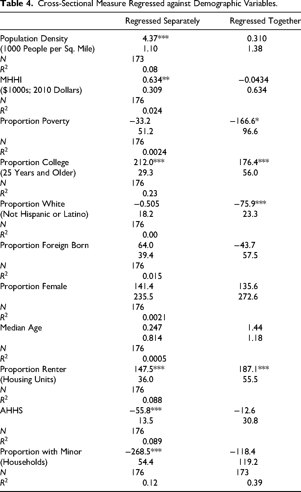
Conforming to hypothesis, population density is significant and positive in the simple regression. This suggests that cities the Cross-Sectional Measure identifies as highly gentrified tend also to be urbanized, rather than being suburban or less dense. As opposed to the Dynamic Measure, this benefits the model if a researcher defines gentrification as occurring in highly urbanized areas. Population density's insignificance in the multiple regressions may suggest that other variables better explain urban characteristics.

The affluence measures (median household income, proportion poverty, and proportion college educated) are all significant in at least one set of regressions and of the expected sign. All three variables are of high magnitude in the regressions in which they are significant. That proportion college educated is highly significant in both sets of regressions helps validate the Dynamic Measure, for which education is integral in construction. Conforming to previous analysis of the Dynamic Measure, but contrary to hypothesis, proportion White is significant and negative in the multiple regression. As mentioned, this might suggest that displacement is not particularly dramatic or that nonwhite neighborhoods are more likely to gentrify. Proportion foreign born is insignificant in both sets of regressions. This runs counter to the hypothesis that this variable would be significant and negative, but conforms to the Dynamic Measure's demographic regressions.

No hypothesis was made for proportion female, and this variable is insignificant in both sets of regressions. Contrary to the hypothesis that median age would be negative (gentrifiers more likely to be younger), this variable is insignificant in both sets of regressions. Because gentrifiers are relatively wealthy, they may be more likely to own residences. However, because they are disproportionally urbanites, they may be more likely to rent. Thus no hypothesis was made for proportion renter. Contrasting analysis of the Dynamic Measure, proportion renter is significant and positive in both sets of regressions, perhaps a measure of urbanization. Conforming to hypothesis, average household size is significant and negative in the simple regression, suggesting that gentrifiers choose to remain single, live in single-family units, or have fewer children. Conforming to hypothesis, proportion with minor is significant and negative in the simple regression, suggesting that gentrifiers choose to have fewer children. Interestingly, average household size and proportion with minor lose significance in the multiple regression.

A Comparison between the Dynamic Measure of Citywide Gentrification and the Cross-Sectional Measure of Citywide Gentrification

Each gentrification measure bears similarities in construction methods. Both variables included in the Cross-Sectional Measure are used in the Dynamic Measure: percentage of older housing and median home value (older housing defined differently). These variables are measured on a tract-by-tract basis for each city. The Dynamic Measure includes two additional variables: median household income and proportion of residents, 25 years or older, with four-year college degrees.

In terms of the variable, older housing, Freeman (2005) argued that abundant older housing in a tract generally signals disinvestment. In terms of the variable, median housing value, Freeman argued that a tract that has not appreciated in real housing value cannot have gentrified. Freeman's argument implies that older housing in gentrifying tracts will have appreciated in value, though much of the older housing will also have been replaced. The Cross-Sectional Measure assumes that older housing may indicate disinvestment, but only if it is inexpensive relative to newer housing in the same city.

As mentioned, the variable, median home value, is included in both the Dynamic and Cross-Sectional Measures. In both models, housing price appreciation indicates the influx of new residents with a higher housing budget. Both models also imply that, in a given tract, appreciating home values may lead to displacement.

For both measures, ungentrified tracts are assumed to be occupied by lower-income residents. For the Dynamic Measure, gentrifiable tracts contain below-median income. For the Cross-Sectional Measure, relatively inexpensive older housing represents dilapidated housing, implying that this housing is occupied by lower-income residents. The measures most fittingly measure urban, not suburban, localities.

Empirical associations were conducted between the Cross-Sectional Measure and the Dynamic Measure. The two measures overlap well. Here considered are 23 cities: those within the top 50 most gentrified by the Cross-Sectional Measure, which have at least 10 percent older housing, and for which the Dynamic Measure indicates a value. Findings show that five of these are in the top 5 percent of cities as assessed by the Dynamic Measure, an additional three are in the top 10 percent, an additional nine are in the top 25 percent, an additional five are in the top 50 percent, and only the remaining one is in the bottom half. This strengthens the case for robustness of each measure.

Figure 1 depicts the correlation between the Cross-Sectional Measure and the Dynamic Measure. Each data point represents a single city. There are 154 cities for which both measures assign a value. For the Dynamic Measure, the mean method is used. The correlation coefficient is 0.48. This graph lends to the notion of a positive relationship between these measures.

Figure A1.

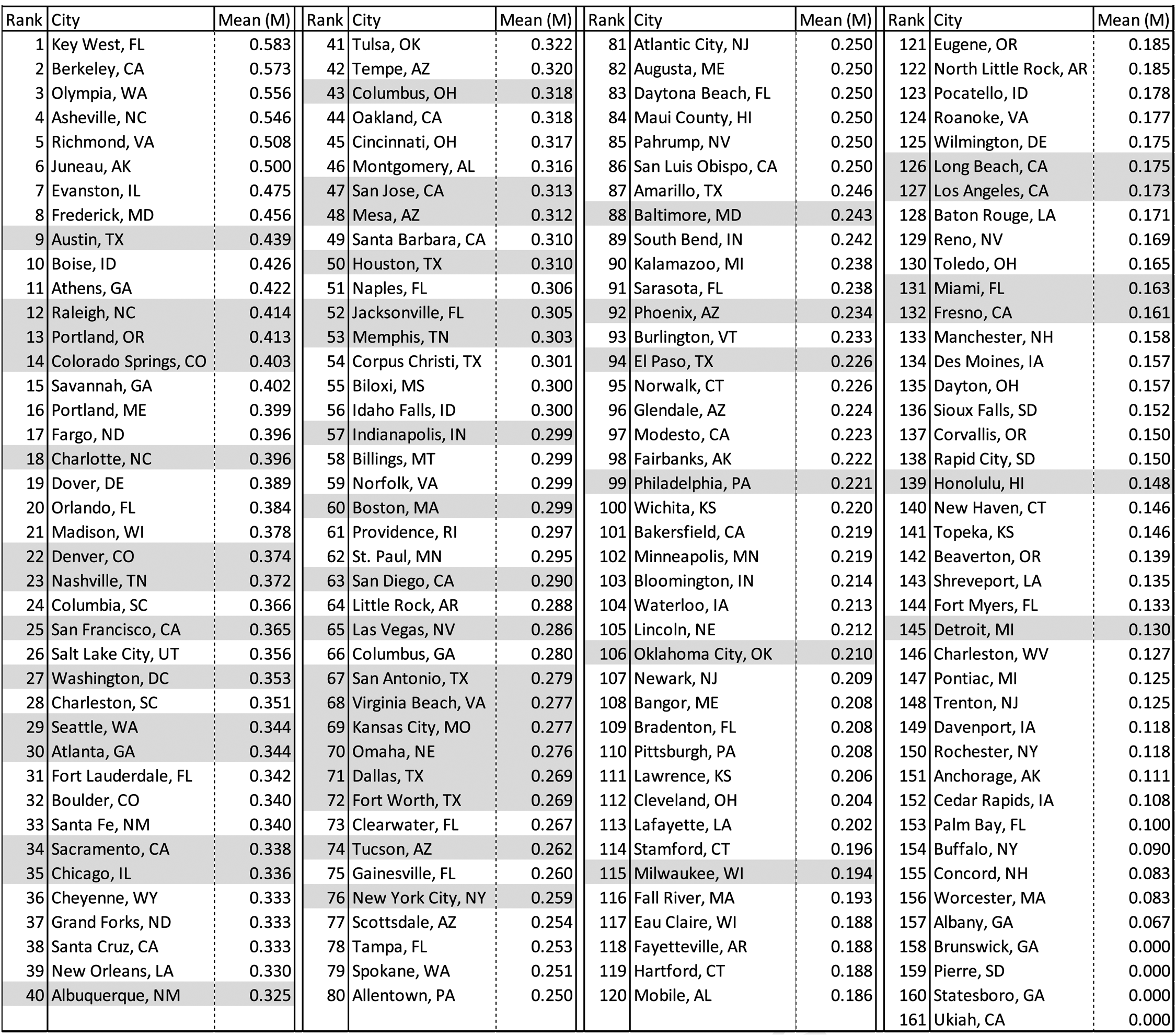
Figure 1. List of cities in order of the Dynamic Measure of the Citywide Gentrification.

Figure 2 plots cities with older housing greater than 10 percent, as assessed by the Cross-Sectional Measure. A total of 85 cities were graphed. The plot tightens, likely because both measures more accurately assess cities with large degrees of older housing. The correlation coefficient here is 0.59. This plot indicates that there is a meaningful association between these measures.

Figure A2.

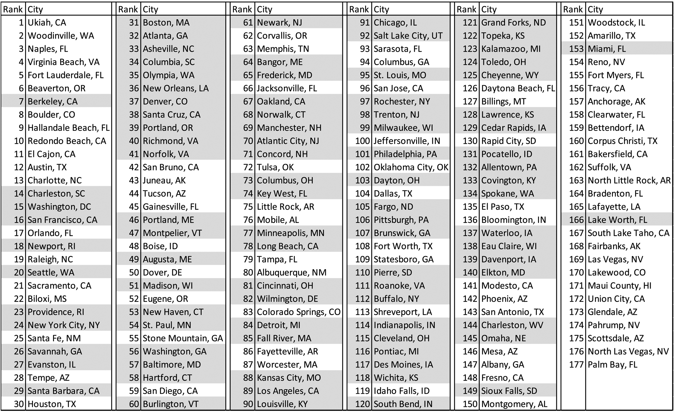
List of cities in order of the Cross-Sectional Measure of the Citywide Gentrification.

The Cross-Sectional Measure was regressed against the Dynamic Measure. The results are very significant, indicating the robustness of each measure. The coefficient is 210, the p-value is 0.00, and the $R^{2}$ is 0.23. The coefficient represents how many ranks a city is likely to ascend in the Cross-Sectional Measure if, by the Dynamic Measure, the city shifts from completely non-gentrified to completely gentrified. This magnitude generally conforms to expectations. The p-value is also promising.

Counter to hypothesis, the Cross-Sectional Measure and the Dynamic Measure are not neatly associated. Several reasons may explain this. First, the relatively low correlation coefficient and $R^{2}$ may actually be reasonable for this type of research. Many studies comparing neighborhood gentrification measures have found that such assessments often yield divergent results (Barton 2014; Galster and Peacock 1986; Preis et al. 2021). Second, this may be explained by the cities with only a few tract observations. Third, the Cross-Sectional Measure functions better when cities have a higher degree of older housing. Fourth, cities with low gentrification scores by the Cross-Sectional Measure tend to have experienced low levels of gentrification, but variation among them is not instructive. Fifth, gentrification has many definitions and components, so each measure may capture different aspects (e.g., demographic shifts vs. housing reinvestment). Sixth, the Dynamic Measure can incorporate suburban transition, while the Cross-Sectional Measure primarily considers urban change. Seventh, these measures were developed in part for their simplicity, and so excluded variables may lessen the statistical relationship.

Devising the Dynamic and Cross-Sectional Measures

A measure may experience tradeoffs: generalizability versus specificity and rigor versus completeness. These measures were constructed in part to be rigorous. Rigor implies the following strengths. First, commonly cited variables are employed. Second, variables are not weighted. Third, the model's construction is straightforward. Fourth, it is clear what the model is measuring. Fifth, although the model is not too simple, neither is it too complex. Sixth, the model is replicable and broadly applicable. Importantly, maximizing rigor is not appropriate for every model. In particular cases, some rigor should be sacrificed in pursuit of other objectives.

The present paper's models exclude certain demographic variables. Population density may indicate urbanization, but urbanization does not strictly imply gentrification. The rate of poverty was excluded because median household income is more widely used than poverty. Proportion renter may be somewhat ambiguous because gentrifiers may rent housing and original residents may own. Finally, there may be only slight variations in average household size, proportion of female residents, or median age. Furthermore, these latter three variables are not often considered essential in conceptualizing gentrification.

Neither measure includes race. However, gentrification often entails sociogeographical racial transition, which may disperse communities, dissolve cultures, as well as destabilize politics, economics, and social dynamics. Shifting neighborhood racial demographics create power inequities. Also, legacies of historical racism, such as redlining and unequal public funding, often frame contemporary gentrification. Finally, spaces and people are valued or devalued based on race, affecting where gentrification occurs (Rucks-Ahidiana 2021). Rucks-Ahidiana stated, “I use the theory of racial capitalism to explain why and how gentrification has always been uneven and unequal by race.” However, the author acknowledged that class-based variables best quantitively assess gentrification. Several reasons underlie the decision to omit race-based variables from the two measures.

First, many authors excluded race when defining gentrification's foundational elements (Freeman 2005; Ley 1986; Smith 1979). Second, race differs in importance geographically and historically. Across cities, the share of White residents varies, particular minorities are more populous, and minority populations are varyingly affluent (US Census Bureau 2024). Also, gentrification's causes and effects may be highly racialized or less so.

Third, many authors found that “on average majority-White neighborhoods have higher rates of gentrification” (Rucks-Ahidiana 2021). Fourth, gentrifying neighborhoods often retain their racial characteristics. White gentrifiers may gentrify majority White neighborhoods, and Black gentrifiers may gentrify majority Black neighborhoods. Additionally, minority gentrifiers may preserve a neighborhood's racial composition (Rucks-Ahidiana 2021).

Fifth, if a measure includes both class- and race-based variables as sufficient conditions for gentrification, the model may obscure which variables determine gentrification. If a measure includes class- and race-based variables as necessary conditions, then race-based variables may exclude some gentrifying cities in which class dynamics dominate. In cities where racial dynamics dominate, gentrifiers are likely to have greater education and purchasing power, and so the present paper's measures likely nevertheless capture gentrification there. Sixth, a model with fewer variables is more rigorous.

Another consideration is that gentrification does not necessarily respect political boundaries. For instance, suburban satellite cities may have experienced demographic and housing transitions. However, both measures delineate by municipal boundaries. Several considerations motivate this approach.

First, the measures are designed to capture urban gentrification. Second, urban areas rarely overlap two cities. Third, if a single city comprises multiple urban regions, the measures capture all urbanized districts. Fourth, some metropolitan areas comprise multiple urban areas in separate municipalities, but the central city usually contains the dominant urban center. Fifth, including suburban satellite cities would greatly vary the urban-to-suburban ratio among cities, which would complicate the models. Sixth, gentrification often reshapes local politics, which may be best studied within a single jurisdiction.

Conclusion

This paper constructed two methods to measure citywide gentrification: the Dynamic Measure of Citywide Gentrification and the Cross-Sectional Measure of Citywide Gentrification. Each measure identifies highly gentrified cities, and the Dynamic Measure also identifies cities with especially low levels of gentrification. Rather than the neighborhood, using the city as the unit of measurement is novel but reasonable given how gentrification is sometimes discussed academically and journalistically. The purpose of this paper is to introduce new ways to conceptualize and measure gentrification, and to identify highly gentrified cities as well as those less gentrified.

Each of these gentrification measurement methods was devised on theoretical grounds, lending credibility to both assessments. Regressing the Cross-Sectional Measure against the Dynamic Measure yields a reasonable magnitude and a p-value of 0.00. Many prominent cities each measure designates as highly gentrified conform to anecdotal accounts, and these cities tend to align between the measures. Cities that the Dynamic Measure identifies to have experienced low gentrification also conform to expectations. Case studies, reports, and local newspapers confirmed that most prominent cities each measure identifies as highly gentrified have experienced gentrification. Many coefficients are significant when these measures are regressed against demographic variables. However, the correlation coefficient when plotting the measures against each other, and the $R^{2}$ when regressing them against each other, are both relatively low. Ultimately, evidence generally supports the robustness of each measure to assess citywide gentrification.

According to this research, highly gentrified cities have over decades experienced gentrification across large portions of their urban areas. A policy implication is that cities should regard gentrification as likely to occur across many downtown neighborhoods, with localized gentrification expanding to nearby areas. Policymakers might anticipate near-term displacement in neighborhoods adjacent to gentrifying areas, and for gentrification to eventually spread farther. Whether publicly or privately provided, construction of physical amenities in one area may eventually affect residents in another.

Local governments may focus on housing to stymie demographic shifts: identifying at-risk areas and initiating or allowing construction of affordable housing. Rent control, eviction restrictions, denser zoning, and permitting accessory dwelling units would also likely slow socioeconomic realignment. Finally, state and HUD policymakers might allocate additional funding to rapidly gentrifying cities.

An analytical implication is that researchers can use data compiled for this paper to conduct cross-city inquiry. This includes statewide, regional, or national investigation. Gentrification statistics can be compared to other citywide variables, and studies can either focus on gentrification or use gentrification metrics as control variables. Furthermore, because two measures have been constructed, one measure can act as a robustness check, potentially bolstering significant results. Also, mixed-methods scholars can select case studies based on these measures’ gentrification scores, for individual investigation or to supplement quantitative analysis. The primary purpose of this paper is to expand researchers’ toolkit.

Future research may further test the viability of these measures by comparing them to other assessments or evaluating their relationship to theoretically related variables. Also, the Dynamic Measure may be mapped onto representative cities. The Cross-Sectional Measure may be estimated for other decades and these cross-decade values compared. Researchers may also use these measures to test for gentrification's relationship to displacement, community dispersal, intracity institutional change (in politics, economics, social relations, culture, amenities, the physical landscape, and grassroots activism), or a plethora of other variables. These operationalizations can benefit myriad avenues of research.

Supplemental Material

sj-xlsx-1-uar-10.1177_10780874261446627 - Supplemental material for Formulation and Evaluation of Two Citywide Gentrification Measures

Supplemental material, sj-xlsx-1-uar-10.1177_10780874261446627 for Formulation and Evaluation of Two Citywide Gentrification Measures by Alex Mozell in Urban Affairs Review

Footnotes

Acknowledgements

I want to thank Michael Ash whose support and insight encouraged this research.

ORCID iD

Alex Mozell

Funding

The author received no financial support for the research, authorship, and/or publication of this article.

Declaration of Conflicting Interests

The author declared no potential conflicts of interest with respect to the research, authorship, and/or publication of this article.

Data Availability

Mozell, Alex. Dynamic and Cross-Sectional Citywide Gentrification Data. figshare, October 3, 2025. doi:10.6084/m9.figshare.30275926.v1.

https://doi.org/10.6084/m9.figshare.30275926

Approval Committee

Michael Ash, Gregor Semieniuk, Ellen Pader, all of the University of Massachusetts Amherst.

Supplemental Material

Supplemental material for this article is available online.

Author Biography

Alex Mozell holds a PhD in economics from the University of Massachusetts Amherst. His research examines the relationship between gentrification and the criminalization of homelessness, emphasizing political and economic structures.

Appendix

References

Aalbers

Manuel B

. 2019. “Introduction to the Forum: From Third to Fifth-Wave Gentrification.” Tijdschrift voor Economische en Sociale Geografie 110 (1): 1–11. https://doi.org/10.1111/tesg.12332 .

Barton

Michael

. 2014. “An Exploration of the Importance of the Strategy Used to Identify Gentrification.” Urban Studies 53 (1): 92–111. https://doi.org/10.1177/0042098014561723 .

Bates

Lisa

. 2013. “Gentrification and Displacement Study: Implementing an Equitable Inclusive Development Strategy in the Context of Gentrification.” City of Portland Bureau of Planning and Sustainability. https://www.portland.gov/sites/default/files/2020-01/2-gentrification-and-displacement-study-05.18.13.pdf.

Berry

Brian J. L.

1985. “Islands of Renewal in Seas of Decay.” In The New Urban Reality, edited by Peterson

Paul E.

, 69–96. Washington, DC: Brookings.

Bostic

Raphael W.

Martin

Richard W.

. 2003. “Black Home-Owners as a Gentrifying Force? Neighbourhood Dynamics in the Context of Minority Home-Ownership.” Urban Studies 40 (12): 2427–49. https://doi.org/10.1080/0042098032000136147 .

Cole

Helen VS

Mehdipanah

Roshanak

Gullón

Pedro

Triguero-Mas

Margarita

. 2021. “Breaking Down and Building Up: Gentrification, Its Drivers, and Urban Health Inequality.” Current Environmental Health Reports 8 (2): 157–66. https://doi.org/10.1007/s40572-021-00309-5 .

Couture

Victor

Handbury

Jessie

. 2023. “Neighborhood Change, Gentrification, and the Urbanization of College Graduates.” Journal of Economic Perspectives 37 (2): 29–52. https://doi.org/10.1257/jep.37.2.29 .

Croff

Raina

Hedmann

Monique

Barnes

Lisa L.

. 2021. “Whitest City in America: A Smaller Black Community’s Experience of Gentrification, Displacement, and Aging in Place.” The Gerontologist 61 (8): 1254–65. https://doi.org/10.1093/geront/gnab041 .

Curran

Winifred

. 2007. “‘From the Frying Pan to the Oven’: Gentrification and the Experience of Industrial Displacement in Williamsburg, Brooklyn.” Urban Studies 44 (8): 1427–40. https://doi.org/10.1080/00420980701373438 .

10.

Davidson

Mark

Lees

Loretta

. 2005. “New-Build ‘Gentrification’ and London’s Riverside Renaissance.” Environment and Planning A: Economy and Space 37 (7): 1165–90. https://doi.org/10.1068/a3739 .

11.

Desmond

Matthew

Gershenson

Carl

. 2017. “Who Gets Evicted? Assessing Individual, Neighborhood, and Network Factors.” Social Science Research 62: 362–77. https://doi.org/10.1016/j.ssresearch.2016.08.017 .

12.

Ding

Lei

Hwang

Jackelyn

Divringi

Eileen

. 2016. “Gentrification and Residential Mobility in Philadelphia.” Regional Science and Urban Economics 61: 38–51. https://doi.org/10.1016/j.regsciurbeco.2016.09.004 .

13.

Easton

Sue

Lees

Loretta

Hubbard

Phil

Tate

Nicholas

. 2020. “Measuring and Mapping Displacement: The Problem of Quantification in the Battle Against Gentrification.” Urban Studies 57 (2): 286–306. https://doi.org/10.1177/0042098019851953 .

14.

Ellen

Ingrid Gould

O’Regan

Katherine M.

. 2011. “How Low Income Neighborhoods Change: Entry, Exit, and Enhancement.” Regional Science and Urban Economics 41 (2): 89–97. https://doi.org/10.1016/j.regsciurbeco.2010.12.005 .

15.

Elliott-Cooper

Adam

Hubbard

Phil

Lees

Loretta

. 2020. “Moving Beyond Marcuse: Gentrification, Displacement and the Violence of Un-Homing.” Progress in Human Geography 44 (3): 492–509. https://doi.org/10.1177/0309132519830511 .

16.

Freeman

Lance

. 2005. “Displacement or Succession? Residential Mobility in Gentrifying Neighborhoods.” Urban Affairs Review 40 (4): 463–91. https://doi.org/10.1177/1078087404273341 .

17.

Freeman

Lance

Braconi

Frank

. 2004. “Gentrification and Displacement New York City in the 1990s.” Journal of the American Planning Association 70 (1): 39–52. https://doi.org/10.1080/01944360408976337 .

18.

Galster

George

Peacock

Stephen

. 1986. “Urban Gentrification: Examining Alternative Indicators.” Social Indicators Research 18 (3): 321–37. https://doi.org/10.1007/BF00286623 .

19.

Ghertner

D. Asher

. 2015. “Why Gentrification Theory Fails in ‘Much of the World’.” Analysis of Urban Change, Theory, Action 19 (4): 552–63. https://doi.org/10.1080/13604813.2015.1051745 .

20.

Gotham

Kevin F

. 2005. “Tourism Gentrification: The Case of New Orleans’ Vieux Carre (French Quarter).” Urban Studies 42 (7): 1099–121. https://doi.org/10.1080/00420980500120881 .

21.

Hammel

Daniel J.

Wyly

Elvin K.

. 1996. “A Model for Identifying Gentrified Areas with Census Data.” Urban Geography 17 (3): 248–68. https://doi.org/10.2747/0272-3638.17.3.248 .

22.

Hamnett

Chris

. 2003. “Gentrification and the Middle-Class Remaking of Inner London, 1961-2001.” Urban Studies 40 (12): 2401–26. https://doi.org/10.1080/0042098032000136138 .

23.

Harvey

David

. 1982. The Limits to Capital. Oxford: Basil Blackwell Ltd.

24.

Holm

Andrej

Schulz

Guido

. 2018. “GentriMap: A Model for Measuring Gentrification and Displacement.” In Gentrification and Resistance: Researching Displacement Processes and Adaption Strategies, edited by Ilse

Helbrecht

, 251–77. Wiesbaden: Springer VS.

25.

Hudalah

Delik

Adharina

Nabilla

. 2019. “Towards a Global View on Suburban Gentrification: From Redevelopment to Development.” Indonesian Journal of Geography 51 (1): 97–105. https://doi.org/10.22146/ijg.34813 .

26.

Hwang

Jackelyn

Sampson

Robert J.

. 2014. “Divergent Pathways of Gentrification: Racial Inequality and the Social Order of Renewal in Chicago Neighborhoods.” American Sociological Review 79 (4): 726–51. https://doi.org/10.1177/0003122414535774 .

27.

Kreager

Derek A.

Lyons

Christopher J.

Hays

Zachary R.

. 2011. “Urban Revitalization and Seattle Crime, 1982-2000.” Social Problems 58 (4): 615–39. https://doi.org/10.1525/sp.2011.58.4.615 .

28.

Lees

Loretta

. 2003. “Super-Gentrification: The Case of Brooklyn Heights, New York City.” Urban Studies 40 (12): 2487–509. https://doi.org/10.1080/0042098032000136174 .

29.

Lees

Loretta

. 2008. “Gentrification and Social Mixing: Towards an Inclusive Urban Renaissance?” Urban Studies 45 (12): 2449–70. https://doi.org/10.1177/0042098008097099 .

30.

Lees

Loretta

Shin

Hyun Bang

López-Morales

Ernesto

. 2016. Planetary Gentrification. Hoboken, NJ: John Wyly & Sons.

31.

Lefebvre

Henri

. 1968. Le Droit à La Ville. Paris: Anthopos.

32.

Ley

David

. 1986. “Alternative Explanations for Inner-City Gentrification: A Canadian Assessment.” Annals of the Association of American Geographers 76 (4): 521–35. https://doi.org/10.1111/j.1467-8306.1986.tb00134.x .

33.

Maciag

Mike

. 2015. Gentrification in America Report. Governing. https://www.governing.com/gov-data/census/gentrification-in-cities-governing-report.html.

34.

Marcuse

Peter

. 1985. “To Control Gentrification: Anti-Displacement Zoning and Planning for Stable Residential Districts.” Review of Law & Social Change 13: 931–52. https://socialchangenyu.com/wp-content/uploads/2019/09/PETER-MARCUSE_RLSC_13.4.pdf

35.

Marcuse

Peter

. 1986. “Abandonment, Gentrification, and Displacement: The Linkages in New York City.” In Gentrification of the City, edited by Smith

Neil

Williams

Peter

, 153–77. London: Routledge.

36.

McKinnish

Terra

Walsh

Randall

White

Kirk T.

. 2010. “Who Gentrifies Low-Income Neighborhoods?” Journal of Urban Economics 67 (2): 180–93. https://doi.org/10.1016/j.jue.2009.08.003 .

37.

Minnesota Population Center. n.d. “Integrated Spatio-Temporal Aggregate Data Series.” https://www.nhgis.org/.

38.

Mozell, Alex. 2025. Dynamic and Cross-Sectional Citywide Gentrification Data. figshare. https://doi.org/10.6084/m9.figshare.30275926.v1.

39.

Papachristos

Andrew V.

Smith

Chris M.

Scherer

Mary L.

Fugiero

Melissa A.

. 2011. “More Coffee, Less Crime? The Relationship Between Gentrification and Neighborhood Crime Rates in Chicago, 1991 to 2005.” City & Community 10 (3): 215–40. https://doi.org/10.1111/j.1540-6040.2011.01371.x .

40.

Preis

Benjamin

Janakiraman

Aarthi

Bob

Alex

Steil

Justin

. 2021. “Mapping Gentrification and Displacement Pressure: An Exploration of Four Distinct Methodologies.” Urban Studies 58 (2): 405–24. https://doi.org/10.1177/0042098020903011 .

41.

Pudlin

Alex

. 2016. “Los Angeles Index of Neighborhood Change.” City of Los Angeles Open Data. https://geohub.lacity.org/datasets/57e9231c3bd34d44ae49b309b0cb440e_1/about.

42.

Pudlin

Alex

. 2018. “Los Angeles Index of Displacement Pressure.” City of Los Angeles Open Data. https://geohub.lacity.org/datasets/lahub::los-angeles-index-of-displacement-pressure/explore?location=34.019685 percent2C-118.412044 percent2C9.53.

43.

Quinton

Jessica

Nesbitt

Lorien

Sax

Daniel

. 2022. “How Well Do We Know Green Gentrification? A Systematic Review of the Methods.” Progress in Human Geography 46 (4): 960–87. https://doi.org/10.1177/03091325221104478 .

44.

Richardson

Jason

Mitchell

Bruce

Edlebi

Jad

. 2020. Gentrification and Disinvestment 2020. National Community Reinvestment Coalition. https://ncrc.org/gentrification20/.

45.

Robiou

Marcia

. 2018. When Gentrification Is a Mental Health Issue. CityLab. https://www.bloomberg.com/news/articles/2018-03-27/gentrification-in-nyc-is-harming-mental-health.

46.

Rucks-Ahidiana

Zawadi

. 2021. “Racial Composition and Trajectories of Gentrification in the United States.” Urban Studies 58 (13): 2721–41. https://doi.org/10.1177/0042098020963853 .

47.

Seattle 2035 Growth and Equity. 2016. Seattle Office of Planning & Community Development. https://www.seattle.gov/Documents/Departments/OPCD/OngoingInitiatives/SeattlesComprehensivePlan/FinalGrowthandEquityAnalysis.pdf.

48.

Seawright

Jason

. 2016. Multi-Method Social Science: Combining Qualitative and Quantitative Tools. Cambridge, UK: Cambridge University Press.

49.

SimplyAnalytics. 2003. New York City, NY.

50.

Slater

Tom

. 2006. “The Eviction of Critical Perspectives from Gentrification Research.” International Journal of Urban and Regional Research 30 (4): 737–57. https://doi.org/10.1111/j.1468-2427.2006.00689.x .

51.

Slater

Tom

Curran

Winifred

Lees

Loretta

. 2004. “Gentrification Research: New Directions and Critical Scholarship.” Environment and Planning A 36 (7): 1141–50. https://doi.org/10.1068/a3718 .

52.

Smith

Darren P.

Phillips

D. A.

. 2001. “Socio-Cultural Representations of Greentrified Pennine Rurality.” Journal of Rural Studies 17 (4): 457–69. https://doi.org/10.1016/S0743-0167(01)00014-6 .

53.

Smith

Neil

. 1979. “Toward a Theory of Gentrification: A Back to the City Movement by Capital, Not People.” Journal of the American Planning Association 45 (4): 538–48. https://doi.org/10.1080/01944367908977002 .

54.

Toplansky

Marshall

López del Río

Karla

Murphy

Ken

. 2019. Gentrification in Los Angeles. NewGeography. https://www.newgeography.com/content/006209-gentrification-los-angeles.

55.

U.S. Census Bureau. 2010a. Demographic and Housing Estimates, American Community Survey 1-Year and 5-Year Estimates, Table DP05.

56.

U.S. Census Bureau. 2010b. Households and Families, American Community Survey 1-Year and 5-Year Estimates, Table S1101.

57.

U.S. Census Bureau. 2010c. Place of Birth by Nativity and Citizenship Status, American Community Survey 1-Year and 5-Year Estimates, Table B05002.

58.

U.S. Census Bureau. 2010d. Selected Characteristics of the Total and Native Populations in the United States, American Community Survey 1-Year and 5-Year Estimates, Table S0601.

59.

U.S. Census Bureau. 2010e. Tenure by Year Structure Built, 1-Year and 5-Year Estimates, Table B25036.

60.

U.S. Census Bureau. 2010f. Value, American Community Survey 1-Year and 5-Year Estimates, Table B25075.

61.

U.S. Census Bureau. 2020. Annual Geographic Information Table, American Community Survey 1-Year and 5-Year Estimates, Table GEOINFO.

62.

U.S. Census Bureau. 2024. American Community Survey 1-Year Estimates.

63.

Walks

R. Alan

Maaranen

Richard

. 2008. “Gentrification, Social Mix and Social Polarization: Testing the Linkages in Large Canadian Cities.” Urban Geography 29 (4): 293–326. https://doi.org/10.2747/0272-3638.29.4.293 .

64.

Yung

Brandon James

Grecia

Elenes

Elias

Renee Roy

Greenberg

Julia

. n.d. Whose Downtown Fresno? Community Perspectives on the Tensions and Tradeoffs of Reinvestment. UC Berkeley Center for Community Innovation, Urban Displacement Project, California Strategic Growth Council. https://www.urbandisplacement.org/wp-content/uploads/2022/03/Fresno.pdf.

65.

Zukin

Sharon

Trujillo

Valerie

Frase

Peter

Jackson

Danielle

Recuber

Tim

Walker

Abraham

. 2009. “New Retail Capital and Neighborhood Change: Boutiques and Gentrification in New York City.” City & Community 8 (1): 47–64. https://doi.org/10.1111/j.1540-6040.2009.01269.x .

Supplementary Material

Please find the following supplemental material available below.

For Open Access articles published under a Creative Commons License, all supplemental material carries the same license as the article it is associated with.

For non-Open Access articles published, all supplemental material carries a non-exclusive license, and permission requests for re-use of supplemental material or any part of supplemental material shall be sent directly to the copyright owner as specified in the copyright notice associated with the article.

0.00 MB

0.13 MB