Existence of minimizers in the geometrically non-linear 6-parameter resultant shell theory with drilling rotations

Abstract

This paper is concerned with the geometrically non-linear theory of 6-parametric elastic shells with drilling degrees of freedom. This theory establishes a general model for shells, which is characterized by two independent kinematic fields: the translation vector and the rotation tensor. Thus, the kinematical structure of 6-parameter shells is identical to that of Cosserat shells. We show the existence of global minimizers for the geometrically non-linear 2D equations of elastic shells. The proof of the existence theorem is based on the direct methods of the calculus of variations essentially using the convexity of the energy in the strain and curvature measures. Since our result is valid for general anisotropic shells, we analyze the particular cases of isotropic shells, orthotropic shells and composite shells separately.

Keywords

Geometrically non-linear elastic shells existence of minimizers 6-parameter resultant shell theory Cosserat shells drill rotations calculus of variations

1. Introduction

In recent years there has been a revived interest in 2D shell models because of unconventional materials and extremely small aspect-to-thickness ratios, such as for instance thin polymeric films or biological membranes. For classical engineering materials and for non-extreme aspect-to-thickness ratios, available 3D FEM codes may readily be used such that the need for a truly 2D shell model does not arise anymore. However, for ultra-thin specimens the application of a 3D constitutive law is not clear at all. In these extreme cases one is led to employ a 2D shell model. This paper is concerned with one such model, the geometrically non-linear resultant theory of shells. We consider the 6-parameter model of shells which involves two independent kinematic fields: the translation vector field and the rotation tensor field (six independent scalar kinematic variables in total). This theory of shells is one of the most general, and it is also very effective in the treatment of complex shell problems, as can be seen from the works [15, 25, 51], among others. The resultant 6-parameter theory of shells was originally proposed by Reissner [55] and it has subsequently been developed considerably. An account of these developments and main achievements have been presented in the books of Libai and Simmonds [32] and Chróścielewski et al. [14]. In this approach, the 2D equilibrium equations and static boundary conditions of the shell are derived exactly by direct through-the-thickness integration of the stresses in the 3D balance laws of linear and angular momentum. The kinematic fields are then constructed on the 2D level using the integral identity of the virtual work principle. Following this procedure, the 2D model is expressed in terms of stress resultants and work-averaged deformation fields defined on the shell base surface. It is interesting that the kinematical structure of 6-parameter shells (involving the translation vector and rotation tensor) is identical to the kinematical structure of Cosserat shells (defined as material surfaces endowed with a triad of rigid directors describing the orientation of points). From this point of view, the 6-parameter theory of shells is related to the shell model proposed initially by the Cosserat brothers [20] and developed by many authors, such as Zhilin [65], Zubov [66], Altenbach and Zhilin [5], Eremeyev and Zubov [26] and Bîrsan and Altenbach [10]. Using the so-called derivation approach, Neff [38, 42] has independently established a Cosserat-type model for initially planar shells (plates) which is very similar to the 6-parameter resultant shell model. A comparison between these two models has been presented in the paper [11], in the case of plates.

On the other hand, we should mention that the kinematic structure of the 6-parameter shell model is different to the kinematic structure of the so-called Cosserat surfaces, which are defined as material surfaces with one or more deformable directors attached to every point (see [4, 6, 7, 35, 56, 57]). For instance, the kinematics of Cosserat surfaces with one deformable director is also characterized by six degrees of freedom (three for the position of material points and three for the orientation and stretch of the material line element through the thickness), which differ from the six degrees of freedom in the 6-parameter resultant shell model.

The topic of existence of solutions for the 2D equations of linear and non-linear elastic shells has been treated in many works. The results that can be found in literature refer to various types of shell model and they employ different techniques; see for example [1, 2, 8, 9, 21, 28, 30, 31, 58 –64]. The method of formal asymptotic expansions is one method of investigation which allows for the derivation and justification of plate and shell models. The existence theory for linear or nonlinear shells is presented in detail in the books of Ciarlet [16 –18], together with many historical remarks and bibliographic references. Another fruitful approach to the existence theory of 2D plate and shell models (obtained as limit cases of 3D models) is the Γ-convergence analysis of thin structures; see for example [41, 43, 45, 47, 48]. No existence theorem has been published in literature yet concerning the geometrically non-linear 6-parameter theory of elastic shells, as far as we are aware. In the case of linear micropolar shells, the existence of weak solutions has recently been proved in [22]. Existence results for the related (very similar) Cosserat-type model of initially planar shells have been established by Neff [38, 42]. In [41, 43, 45], the linearized version of this model has been analyzed and compared with the classical membrane and bending plate models given by the Reissner–Mindlin and Kirchhoff–Love theories.

In the present work, we prove the existence of minimizers for the minimization problem of the total potential energy associated to the deformation of geometrically non-linear 6-parameter elastic shells. We wish to emphasize that our work is not concerned with the derivation of the 2D shell model, but it presents existence results for the well-established 2D theory of 6-parameter elastic shells. It should be mentioned from the beginning that this model refers to shells made of a simple (classical) elastic material, not a generalized (Cosserat or micropolar) continuum. However, the rotation tensor field appears naturally in this theory, in the course of the exact through-the-thickness reduction of the 3D formulation of the problem to the 2D one [14, 24, 32]. Thus, in spite of the above-mentioned similarity to the kinematics of Cosserat shells, the material of the shell in the resultant 6-parameter model is described as a simple continuum (without any specific microstructure or material length scale). On the other hand, in the case of dimensional reduction of the 3D equations of micropolar shell-like bodies one can obtain the same 6-parameter theory with modified 2D constitutive equations; see for example [3] for the linear case and [38, 42, 67] for the nonlinear case. One can also obtain more complex theories, as in [27].

For the proof of existence, we employ the direct methods of the calculus of variations and extend the techniques presented in [38, 42] to the case of general shells (with non-vanishing curvature in the reference configuration). In Section 2 we briefly present the kinematics of general 6-parameter shells and the equations of equilibrium. In Section 3 we give some alternative formulae for the strain tensor and curvature tensor, which are written in direct tensorial notation as well as in component (matrix) notation. These expressions are needed subsequently in the proof of our main result. In Section 4 we formulate the two-field minimization problem for general elastic shells, corresponding to mixed-type boundary conditions. Under the assumptions of convexity and coercivity of the quadratic strain energy function (physically linear material response), we prove the existence of minimizers over a large set of admissible pairs. Thus, the minimizing solution pair is of class $H^{1} (ω, ℝ^{3})$ for the translation vector and H ¹(ω, SO(3)) for the rotation tensor. The existence result is valid for general anisotropic elastic shells having a reference configuration with arbitrary geometry. Section 5 includes some applications of the existence theorem and discussions of special cases. We present a convenient way to choose the initial directors and the parametrization of the reference surface. Then, we consider the cases of isotropic shells, orthotropic shells, and composite layered shells separately and we present the respective forms of the strain energy densities. Applying the theorem stated previously, we establish the conditions on the constitutive coefficients that ensure the existence of minimizers in each situation. This analysis shows the usefulness of our theoretical result in the treatment of practical problems for elastic shells.

2. General 6-parameter resultant shells

Consider a general 6-parameter shell and denote the base surface of the shell in the reference (initial) configuration as S⁰ and the base surface in the deformed configuration as S. Let O be a fixed point in the Euclidean space and { e ₁, e ₂, e ₃} be the fixed orthonormal vector basis. The reference configuration is represented by the position vector y ⁰ (relative to the point O) of the base surface S⁰ plus the structure tensor Q ⁰. The structure tensor is a second-order proper orthogonal tensor which can be described by an orthonormal triad of directors ${d_{1}^{0}, d_{2}^{0}, d_{3}^{0}}$ attached to every point [14, 24]. Thus the reference (initial) configuration is characterized by the functions

\begin{array}{l} y^{0} : ω \subset ℝ^{2} \to ℝ^{3}, y^{0} = y^{0} (x_{1}, x_{2}), \\ Q^{0} : ω \subset ℝ^{2} \to S O (3), Q^{0} = d_{i}^{0} (x_{1}, x_{2}) \otimes e_{i}, \end{array}

(1)

where (x₁, x₂) are material curvilinear coordinates on the surface S⁰. Throughout the paper Latin indexes i,j,… take the values {1, 2, 3}, while Greek indexes α, β, … take the values {1, 2}. The usual Einstein summation convention over repeated indexes is employed. We assume that the curvilinear coordinates (x₁, x₂) ∊ ω range over a bounded open domain ω (with Lipschitz boundary ∂ω) of the Ox₁x₂ plane (see Figure 1). Let us denote the partial derivative with respect to x_α by ∂_αf = ∂f/∂x_α, for any function f. We designate { a ₁, a ₂} to be the (covariant) base vectors in the tangent plane of S⁰ and n ⁰ to be the unit normal to S⁰, given by

a_{α} = \partial_{α} y^{0} = \frac{\partial y^{0}}{\partial x_{α}}, n^{0} = \frac{a_{1} \times a_{2}}{‖ a_{1} \times a_{2} ‖} .

(2)

Figure 1.

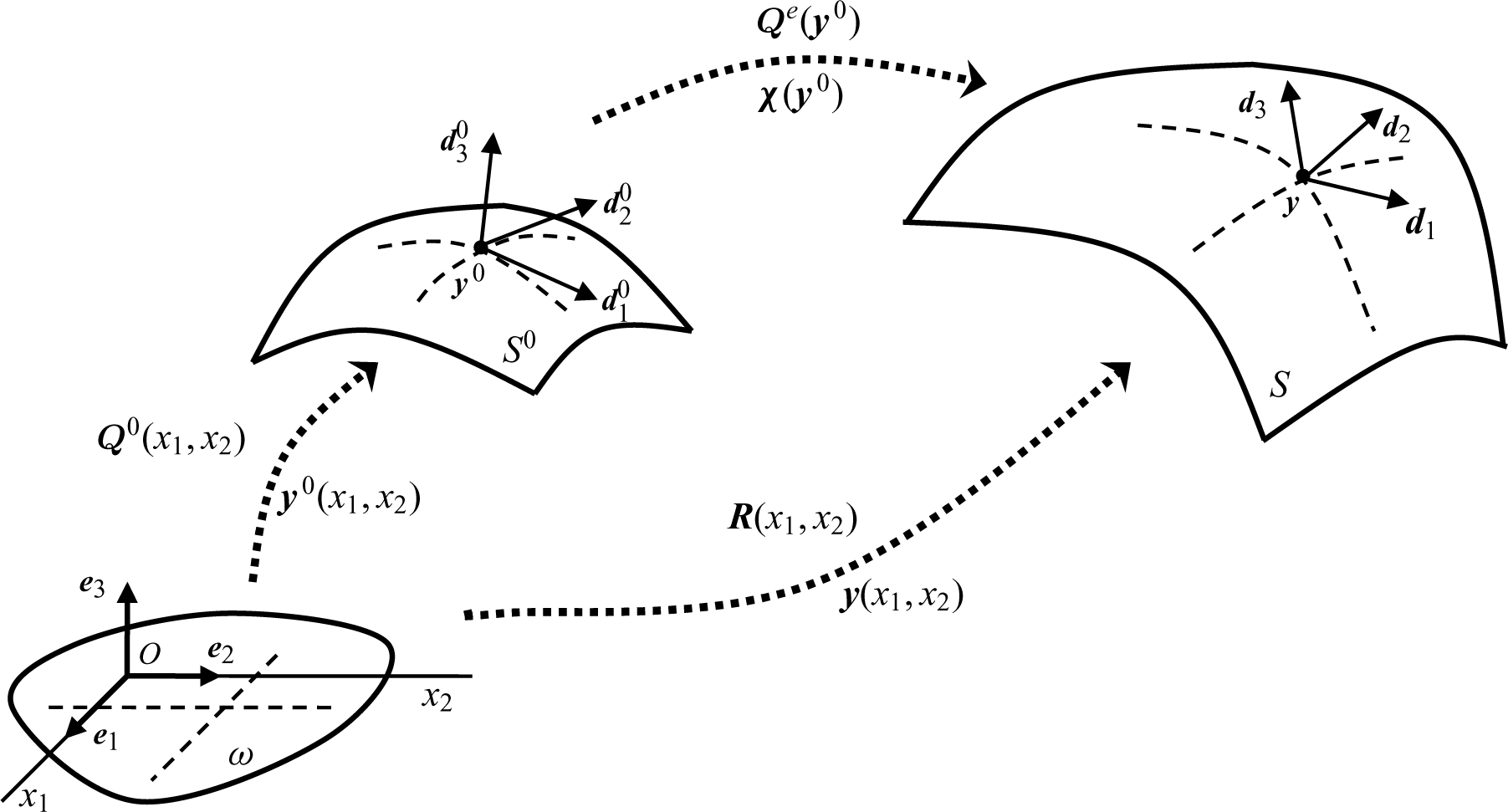
The base surface S⁰ of the shell in the initial configuration, the base surface S in the deformed configuration, and the fictitious planar reference configuration ω. The orthonormal triads of vectors {e_i}, ${d_{i}^{0}}$ and { d _i} are related through the relations $d_{i} = Q^{e} d_{i}^{0} = R e_{i}$ and $d_{i}^{0} = Q^{0} e_{i}$ , where Q ^e is the elastic rotation field, Q ⁰ is the initial rotation, and R is the total rotation field.

The reciprocal (contravariant) basis { a ¹, a ²} of the tangent plane is defined by $a^{α} \cdot a_{β} = δ_{β}^{α}$ (the Kronecker symbol). We also use the notations

a_{3} = a^{3} = n^{0}, a_{α β} = a_{α} \cdot a_{β}, a^{α β} = a^{α} \cdot a^{β}, a = \sqrt{\det {(a_{α β})}_{2 \times 2}} > 0 .

For the deformed configuration of the shell, let y (x₁, x₂) denote the position vector (relative to O) and let { d _i(x₁, x₂)} be the orthonormal triad of directors attached to the point with initial curvilinear coordinates (x₁, x₂). The deformed configuration is completely characterized by the functions

y = χ (y^{0}), Q^{e} = d_{i} \otimes d_{i}^{0} \in S O (3),

(3)

where $χ : S^{0} \to ℝ^{3}$ represents the deformation of the base surface, and the proper orthogonal tensor field Q ^e is the (effective) elastic rotation. The displacement vector is defined as usual by u = y − y ⁰.

The role of the triads of directors ${d_{i}^{0}}$ and { d _i} is to determine the structure tensor Q ⁰ and the rotation tensor Q ^e of the shell respectively. Thus, the directors do not describe here any microstructure of the material. According to the derivation procedure of the 6-parameter shell model, the kinematical fields y and Q ^e are uniquely defined as the work-conjugate averages of 3D deformation distribution over the shell thickness, whose virtual values enter the virtual work principle of the shell (see [14, 33]).

In view of (1) and (3), the deformed configuration can alternatively be characterized by the functions

y = y (x_{1}, x_{2}) = χ (y^{0} (x_{1}, x_{2})), R (x_{1}, x_{2}) = Q^{e} Q^{0} = d_{i} (x_{1}, x_{2}) \otimes e_{i} \in S O (3),

where the vector y and the orthogonal tensor R are fields defined over ω. The orthogonal tensor field Q ^e represents the elastic rotation tensor between the reference and deformed configurations [52, 53]. The tensor Q ⁰ is the initial rotation field, while R = Q ^e Q ⁰ describes the total rotation from the fictitious planar reference configuration ω (endowed with the triad { e _i}) to the deformed configuration S. The tensors Q ⁰ and R are also called the structure tensors of the reference and deformed configurations respectively [14, 24]. The following relations hold

Q^{e} = R Q^{0, T}, d_{i}^{0} = Q^{0} e_{i}, d_{i} = Q^{e} d_{i}^{0} = R e_{i} .

(4)

Usually, the initial directors $d_{i}^{0}$ are chosen such that $d_{3}^{0} = n^{0}$ and $d_{α}^{0}$ belong to the tangent plane of S⁰ (see Remark 10). This assumption is not necessary in general and we do not use it in the proof of our existence result.

Let F = Grad_s y = ∂_α y ⊗ a ^α denote the (total) shell deformation gradient tensor. The strong form of the equations of equilibrium for 6-parameter shells can be written in the form [24]

{Div}_{s} N + f = 0, {Div}_{s} M + axl (N F^{T} - F N^{T}) + c = 0,

(5)

where N and M are the internal surface stress resultant and stress couple tensors of the first Piola–Kirchhoff type, while f and c are the external surface resultant force and couple vectors applied to points of S, but measured per unit area of S⁰. The operators Grad_s and Div_s are the surface gradient and surface divergence respectively, defined intrinsically in [29, 34]. The superscript (·)^T denotes the transpose and axl(·) represents the axial vector of a skew-symmetric tensor.

Let ν be the external unit normal vector to the boundary curve ∂S⁰ lying in the tangent plane. We consider boundary conditions of the type [23, 51]

\begin{matrix} N ν = n^{*}, M ν = m^{*} along \partial S_{f}^{0}, \\ y = y^{*}, R = R^{*} along \partial S_{d}^{0}, \end{matrix}

(6)

where $\partial S^{0} = \partial S_{f}^{0} \cup \partial S_{d}^{0}$ is a disjoint partition of S⁰ ( $\partial S_{f}^{0} \cap \partial S_{d}^{0} = \emptyset$ ) with length $(\partial S_{d}^{0}) > 0$ . Here, n * and m * are the external boundary resultant force and couple vectors respectively, applied along the deformed boundary ∂S, but measured per unit length of $\partial S_{f}^{0} \subset \partial S^{0}$ . We denote by ∂ω_f and ∂ω_d the subsets of the boundary curve ∂ω which correspond to $\partial S_{f}^{0}$ and $\partial S_{d}^{0}$ respectively, through the mapping y ⁰.

The weak form associated to these local balance equations for shells has been presented in [14, 23, 32].

3. Elastic shell strain and curvature measures

According to [14, 24], the elastic shell strain tensor E ^e in the material representation is given by

E^{e} = Q^{e, T} {Grad}_{s} y - {Grad}_{s} y^{0} = (Q^{e, T} \partial_{α} y - \partial_{α} y^{0}) \otimes a^{α},

(7)

since Grad_s y = ∂_α y ⊗ a ^α. It is useful to write the strain tensor E ^e in the alternative form

\begin{array}{l} E^{e} & = & (Q^{e, T} \partial_{α} y - a_{α}) \otimes a^{α} = (Q^{e, T} \partial_{α} y \otimes a^{α} + n^{0} \otimes a^{3}) - (a_{i} \otimes a^{i}) \\ = & (Q^{e, T} \partial_{α} y \otimes e_{α} + n^{0} \otimes e_{3}) (e_{i} \otimes a^{i}) - 11_{3}, \end{array}

or equivalently, since ( e _i ⊗ a ⁱ) = ( a _i ⊗ e _i)⁻¹,

\begin{array}{l} E^{e} = (Q^{e, T} \partial_{α} y \otimes e_{α} + n^{0} \otimes e_{3}) {(a_{i} \otimes e_{i})}^{- 1} - 11_{3} = {\bar{U}}^{e} - 11_{3}, \\ with {\bar{U}}^{e} = (Q^{e, T} \partial_{α} y \otimes e_{α} + n^{0} \otimes e_{3}) {(a_{i} \otimes e_{i})}^{- 1}, \end{array}

(8)

where 11₃ = e _i ⊗ e _i is the identity tensor and ${\bar{U}}^{e}$ represents the non-symmetric elastic shell stretch tensor, which can be seen as the 2D analog of the 3D non-symmetric Biot-type stretch tensor [44] or the first Cosserat deformation tensor [20, p. 123, eq. (43)] for the shell. Let us denote by P the tensor defined by

P = a_{i} \otimes e_{i} = \partial_{α} y^{0} \otimes e_{α} + n^{0} \otimes e_{3} .

(9)

Then, from (8) and (9) we get

\begin{array}{l} E^{e} = {\bar{U}}^{e} - 11_{3} = Q^{e, T} (\partial_{α} y \otimes e_{α} + Q^{e} n^{0} \otimes e_{3}) P^{- 1} - 11_{3}, \\ {\bar{U}}^{e} = Q^{e, T} (\partial_{α} y \otimes e_{α} + Q^{e} n^{0} \otimes e_{3}) P^{- 1} . \end{array}

(10)

In the sequel, it is useful to write the elastic shell strain tensors in component form, relative to the fixed tensor basis { e _i ⊗ e _j}. Let $E^{e} = {(E_{i j}^{e})}_{3 \times 3}$ be the matrix of components for the tensor $E^{e} = E_{i j}^{e} e_{i} \otimes e_{j}$ . In general, we decompose any second-order tensor T in the form T = T_ij e _i ⊗ e _j and denote the matrix of components by T = (T_ij)_3×3 Also, for any vector v = v_i e _i we denote the column matrix of components by v = (v_i)_3×1.

Remark 1 The matrix of components P = (P_ij)_3×3 for the tensor defined in (9) can be specified in terms of its three column vectors as follows

P = {(\partial_{1} y^{0} | \partial_{2} y^{0} | n^{0})}_{3 \times 3} = {(\nabla y^{0} | n^{0})}_{3 \times 3} = {(a_{1} | a_{2} | n^{0})}_{3 \times 3} .

(11)

The tensor P introduced in equation (9) can be seen as a 3D (deformation) gradient

\begin{array}{l} P = \nabla Θ {(x_{1}, x_{2}, x_{3})}_{| x_{3} = 0}, with \\ Θ (x_{1}, x_{2}, x_{3}) : = y^{0} (x_{1}, x_{2}) + x_{3} n^{0} (x_{1}, x_{2}), \end{array}

(12)

and it satisfies $\det P = \sqrt{\det a_{α β}} = a > 0$ , such that the inverse P ⁻¹ exists. The mapping $Θ : ω \times (- \frac{h}{2}, \frac{h}{2}) \to ℝ^{3}$ has been introduced previously in [18, 19, 38], and employed for the geometrical description of 3D shells (h denotes the thickness of the shell).

By virtue of equations (8) and (9), we obtain the following matrix form for the strain tensor E ^e

E^{e} = (Q^{e, T} \partial_{1} y | Q^{e, T} \partial_{2} y | n^{0}) P^{- 1} - 11_{3},

(13)

where 11₃ = (δ_ij)_3×3 is the unit matrix. Equivalently, the matrix E^e can be written as

\begin{array}{l} E^{e} = Q^{e, T} (\partial_{1} y | \partial_{2} y | Q^{e} n^{0}) P^{- 1} - 11_{3}, or \\ E^{e} = {\bar{U}}^{e} - 11_{3} = Q^{e, T} F^{e} - 11_{3} = Q^{e, T} \bar{F} P^{- 1} - 11_{3}, \end{array}

(14)

with

\begin{array}{l} {\bar{U}}^{e} = Q^{e, T} (\partial_{1} y | \partial_{2} y | Q^{e} n^{0}) P^{- 1} = Q^{e, T} (\nabla y | Q^{e} n^{0}) P^{- 1}, \\ F^{e} : = (\partial_{1} y | \partial_{2} y | Q^{e} n^{0}) P^{- 1} = (\nabla y | Q^{e} n^{0}) {(\nabla Θ (x_{1}, x_{2}, 0))}^{- 1}, \\ \bar{F} : = (\partial_{1} y | \partial_{2} y | Q^{e} n^{0}) = (\nabla y | Q^{e} n^{0}), \\ F^{0} : = P = (\partial_{1} y^{0} | \partial_{2} y^{0} | n^{0}) = (\nabla y^{0} | n^{0}), \\ \bar{F} = F^{e} F^{0} . \end{array}

(15)

In order to see a parallel with the classical multiplicative decomposition into elastic and plastic parts from finite elasto-plasticity [37, 40], we may interpret F^e as an elastic shell mid-surface deformation gradient and F⁰ = P as an initial deformation gradient. Both are gradients of suitably defined mappings (see Remark 2 and Figure 2), in contrast to the case of elasto-plasticity. In our context, the elastic material response is defined in terms of the elastic part of the deformation, for example E^e = Q^e,TF^e − 11₃ (cf. (14)).

Figure 2.

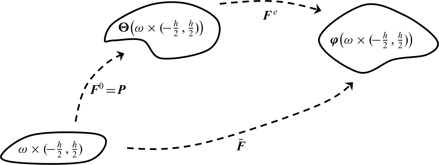
Multiplicative decomposition of the total deformation gradient $\bar{F} = F^{e} F^{0}$ into the elastic shell deformation gradient F^e and the initial deformation gradient F⁰ = P. Interpretation is in terms of reconstructed three-dimensional quantities. The elastic response is governed by F^e. The curved initial configuration corresponds to the intermediate stress-free configuration in multiplicative plasticity.

Remark 2 Although the resultant shell model is truly a 2D theory, we may always consider artificially reconstructed 3D quantities. In this sense, similarly to the context of Remark 1, the tensor $\bar{F} = \partial_{α} y \otimes e_{α} + Q^{e} n^{0} \otimes e_{3}$ , which has the matrix of components $\bar{F}$ , is a 3D deformation gradient

\begin{matrix} \bar{F} = \nabla φ {(x_{1}, x_{2}, x_{3})}_{| x_{3} = 0}, with \\ φ (x_{1}, x_{2}, x_{3}) : = y (x_{1}, x_{2}) + x_{3} Q^{e} (x_{1}, x_{2}) n^{0} (x_{1}, x_{2}) \\ = y (x_{1}, x_{2}) + x_{3} Q^{e} (x_{1}, x_{2}) \nabla Θ (x_{1}, x_{2}, 0) e_{3} . \end{matrix}

(16)

Here, the mapping $φ : ω \times (- \frac{h}{2}, \frac{h}{2}) \to ℝ^{3}$ is a 3D deformation of the body, in terms of the given 2D quantities y (x₁,x₂) and Q ^e(x₁,x₂). Similarly,

\begin{array}{l} F^{e} : = \nabla φ^{e} (Θ {(x_{1}, x_{2}, x_{3})}_{| x_{3} = 0}), with \\ φ^{e} (Θ (x_{1}, x_{2}, x_{3})) : = φ (x_{1}, x_{2}, x_{3}) . \end{array}

However, we note that $\bar{F}$ cannot be interpreted as the 3D deformation gradient of the real 3D shell, because in general the initial normals become arbitrarily curved after deformation.

In terms of the total rotation R and the initial rotation Q ⁰, the elastic shell strain tensor is expressed by

E^{e} = Q^{0} (R^{T} \partial_{α} y - Q^{0, T} \partial_{α} y^{0}) \otimes a^{α} .

(17)

Then, we have

E^{e} = Q^{0} [(R^{T} \partial_{α} y - Q^{0, T} \partial_{α} y^{0}) \otimes e_{α}] (e_{i} \otimes a^{i}) = Q^{0} [(R^{T} \partial_{α} y - Q^{0, T} \partial_{α} y^{0}) \otimes e_{α}] P^{- 1}

which can be written in matrix form as follows

E^{e} = Q^{0} H P^{- 1} with H : = {(R^{T} \partial_{1} y - Q^{0, T} \partial_{1} y^{0} | R^{T} \partial_{2} y - Q^{0, T} \partial_{2} y^{0} | 0)}_{3 \times 3} .

(18)

On the other hand, the elastic shell curvature tensor K ^e in the material description is defined by [14, 24]

K^{e} = [Q^{e, T} axl (\partial_{α} R R^{T}) - axl (\partial_{α} Q^{0} Q^{0, T})] \otimes a^{α} .

(19)

In order to write K ^e in a form more convenient to us, we use relations of the type

{\tilde{Q}}^{T} axl (\partial_{α} \tilde{Q} {\tilde{Q}}^{T}) = axl ({\tilde{Q}}^{T} \partial_{α} \tilde{Q}), axl (\tilde{Q} A {\tilde{Q}}^{T}) = \tilde{Q} axl (A),

(20)

which hold true for any orthogonal tensor $\tilde{Q} \in S O (3)$ and any skew-symmetric tensor $A \in s o (3)$ (see e.g. [12]). Using (20) in (19) we can write the elastic curvature tensor K ^e in the equivalent forms

K^{e} = Q^{e, T} axl (\partial_{α} Q^{e} Q^{e, T}) \otimes a^{α} = axl (Q^{e, T} \partial_{α} Q^{e}) \otimes a^{α},

(21)

K^{e} = [axl (Q^{e, T} \partial_{α} Q^{e}) \otimes e_{α}] {(a_{i} \otimes e_{i})}^{- 1} = [axl (Q^{e, T} \partial_{α} Q^{e}) \otimes e_{α}] P^{- 1} .

Then, the matrix of components $K^{e} = {(K_{i j}^{e})}_{3 \times 3}$ is given by

K^{e} = (axl (Q^{e, T} \partial_{1} Q^{e}) | axl (Q^{e, T} \partial_{2} Q^{e}) | 0) P^{- 1} .

(22)

If we express K ^e in terms of the total rotation R and the initial rotation Q ⁰, we get

K^{e} = Q^{0} [axl (R^{T} \partial_{α} R) - axl (Q^{0, T} \partial_{α} Q^{0})] \otimes a^{α} .

(23)

This relation can be written as

\begin{matrix} K^{e} = K - K^{0}, with K : = Q^{0} axl (R^{T} \partial_{α} R) \otimes a^{α}, \\ K^{0} : = Q^{0} axl (Q^{0, T} \partial_{α} Q^{0}) \otimes a^{α} = axl (\partial_{α} Q^{0} Q^{0, T}) \otimes a^{α}, \end{matrix}

(24)

where the tensor K is the total curvature tensor, while K ⁰ is the initial curvature (or structure curvature tensor of S⁰). In view of (23) and (24), the matrix $K^{e} = (K_{i j}^{e})$ . is given by

\begin{matrix} K^{e} = Q^{0} L P^{- 1} = K - K^{0} with \\ L : = {(axl (R^{T} \partial_{1} R) - axl (Q^{0, T} \partial_{1} Q^{0}) | axl (R^{T} \partial_{2} R) - axl (Q^{0, T} \partial_{2} Q^{0}) | 0)}_{3 \times 3}, \\ K = Q^{0} (axl (R^{T} \partial_{1} R) | axl (R^{T} \partial_{2} R) | 0) P^{- 1}, \\ K^{0} = Q^{0} (axl (Q^{0, T} \partial_{1} Q^{0}) | axl (Q^{0, T} \partial_{2} Q^{0}) | 0) P^{- 1} . \end{matrix}

(25)

In what follows, we shall use the expressions (18) and (25) of the elastic shell strain measures E ^e and K ^e written with tensor components in the basis { e _i ⊗ e _j}.

Remark 3 As expected, the case of zero strain and bending measures corresponds to a rigid body mode of the shell. Indeed, if E ^e = 0 and K ^e = 0 , then from (7) and (21) we obtain

\partial_{α} y = Q^{e} \partial_{α} y^{0} and \partial_{α} Q^{e} = 0 .

Hence, it follows that Q ^e is constant and

y = Q^{e} y^{0} + c (c = constant),

which means that the shell undergoes a rigid body motion with constant translation c and constant rotation Q ^e.

Remark 4 In the case where the base surface S⁰ of the initial configuration of the shell is planar we may assume that S⁰ coincides with ω. In this situation we have a _i = e _i, P = 11₃, and the above strain and curvature measures coincide with those defined for the Cosserat model of planar shells introduced in [38, 42].

Remark 5 In view of (21) and (22), the elastic shell curvature tensor K ^e is an analog of the second Cosserat deformation tensor in the 3D theory: see the original Cosserat book [20, p. 123, eq. (44)].

4. Variational formulation for elastic shells

Let us denote the strain energy density of the elastic shell by W = W( E ^e, K ^e). According to the hyperelasticity assumption, the internal surface stress resultant N and stress couple tensor M are expressed by the constitutive equations in the form

N = Q^{e} \frac{\partial W}{\partial E^{e}}, M = Q^{e} \frac{\partial W}{\partial K^{e}} .

(26)

In this paper we assume that the strain energy density W is a quadratic function of its arguments E ^e and K ^e. Thus, the considered model is physically linear and geometrically non-linear. The explicit form of the strain energy function W is presented in [24, 32] for isotropic, hemitropic or orthotropic elastic shells. In general, the coefficients of the strain energy function W depend on the structure curvature tensor K ⁰ (see [24]). In [13], the case of composite (layered) shells is investigated and the expression of the energy density is established. These special cases will be discussed in Section 5.

Consider the usual Lebesgue spaces $(L^{p} (ω), ‖ \cdot ‖_{L^{p} (ω)}), p \geq 1$ , and Sobolev space $(H^{1} (ω), ‖ \cdot ‖_{H^{1} (ω)})$ . We denote by $L^{p} (ω, ℝ^{3})$ (and respectively $H^{1} (ω, ℝ^{3})$ ) the space of all vector fields v = v_i e _i such that v_i ∊ L^p(ω) (and respectively v_i ∊ H¹(ω)). Similarly, we denote the following sets

\begin{matrix} H^{1} (ω, ℝ^{3 \times 3}) = {T = T_{i j} e_{i} \otimes e_{j} | T_{i j} \in H^{1} (ω)}, \\ H^{1} (ω, S O (3)) = {T \in H^{1} (ω, ℝ^{3 \times 3}) | T \in S O (3)}, \\ L^{p} (ω, ℝ^{3 \times 3}) = {T = T_{i j} e_{i} \otimes e_{j} | T_{i j} \in L^{p} (ω)}, \\ L^{p} (ω, S O (3)) = {T \in L^{p} (ω, ℝ^{3 \times 3}) | T \in S O (3)} . \end{matrix}

The norm of a tensor T is defined by ‖ T ‖² = tr( TT ^T) = T_ijT_ij.

Concerning the boundary-value problem of (5) and (6), we assume the existence of a function Λ( y , R ) representing the potential of external surface loads f , c , and boundary loads n *, m * (cf. [23]).

We consider the following two-field minimization problem associated to the deformation of elastic shells: find the pair $(\hat{y}, \hat{R})$ in the admissible set $A$ which realizes the minimum of the functional

I (y, R) = \int_{S^{0}} W (E^{e}, K^{e}) d S - Λ (y, R) for (y, R) \in A

(27)

where dS is the area element of the surface S⁰. The admissible set $A$ is defined by

A = {(y, R) \in H^{1} (ω, ℝ^{3}) \times H^{1} (ω, S O (3)) | y_{| \partial S_{d}^{0}} = y^{*}, R_{| \partial S_{d}^{0}} = R^{*}},

(28)

where the boundary conditions are to be understood in the sense of traces. The tensors E ^e and K ^e are expressed in terms of ( y , R ) through the relations (17) and (23). If we write $W = W (E^{e}, K^{e}) = \tilde{W} (\nabla y, R, \nabla R)$ , then, referring the integral to the (fictitious reference) domain ω, the change-of-variable formula clearly gives

\begin{array}{l} \int_{S^{0}} W (E^{e}, K^{e}) d S = \int_{ω} W (E^{e}, K^{e}) a (x_{1}, x_{2}) d x_{1} d x_{2} \\ = \int_{ω} \tilde{W} (\nabla y (x_{1}, x_{2}), R (x_{}, x_{2}), \nabla R (x_{1}, x_{2})) det (\nabla Θ (x_{1}, x_{2}, 0)) d x_{1} d x_{2}, \end{array}

(29)

where $a = \sqrt{\det (a_{α β})}$ is the notation introduced previously. The variational principle for the total energy of elastic shells with respect to the functional (27) has been presented in [23, Section 2]. We decompose the loading potential Λ( y , R ) additively as follows

\begin{matrix} Λ (y, R) = Λ_{S^{0}} (y, R) + Λ_{\partial S_{f}^{0}} (y, R), \\ Λ_{S^{0}} (y, R) = \int_{S^{0}} f \cdot u d S + Π_{S^{0}} (R), Λ_{\partial S_{f}^{0}} (y, R) = \int_{\partial S_{f}^{0}} n^{*} \cdot u d l + Π_{\partial S_{f}^{0}} (R), \end{matrix}

(30)

where u = y − y ⁰ is the displacement vector and d l is the element of length along the boundary curve $\partial S_{f}^{0}$ . In (30), $Λ_{S^{0}} (y, R)$ is the potential of the external surface loads f , c , while $Λ_{\partial S_{f}^{0}} (y, Q^{e})$ is the potential of the external boundary loads n *, m *. The expressions of the load potential functions $Π_{S^{0}}, Π_{\partial S_{f}^{0}} : L^{2} (ω, S O (3)) \to ℝ$ are not given explicitly, but they are assumed to be continuous and bounded operators. Of course, the integrals over S⁰ and $\partial S_{f}^{0}$ appearing in (30) can be transformed as in (29) into integrals over ω and ∂ω_f, respectively.

One can consider more general cases of external loads in the definition of the loading potential (30), such as for example tracking loads.

4.1. Main result: Existence of minimizers

This theorem states the existence of minimizers to the minimization problem (27)–(30).

Theorem 6 Assume that the external loads satisfy the conditions

f \in L^{2} (ω, ℝ^{3}), n^{*} \in L^{2} (\partial ω_{f}, ℝ^{3}),

(31)

and the boundary data satisfy the conditions

y^{*} \in H^{1} (ω, ℝ^{3}), R^{*} \in H^{1} (ω, S O (3)) .

(32)

Assume that the following conditions concerning the initial configuration are fulfilled: $y^{0} : ω \subset ℝ^{2} \to ℝ^{3}$ is a continuous injective mapping and

\begin{matrix} y^{0} \in H^{1} (ω, ℝ^{3}), Q^{0} \in H^{1} (ω, S O (3)), \end{matrix}

(33)

\begin{matrix} a_{α} = \partial_{α} y^{0} \in L^{\infty} (ω, ℝ^{3}) (i . e . \nabla y^{0} \in L^{\infty} (ω, ℝ^{3 \times 2})), \\ \det (a_{α β} (x_{1}, x_{2})) \geq a_{0}^{2} > 0, \end{matrix}

(34)

where a₀ is a constant. The strain energy density W( E ^e, K ^e) is assumed to be a quadratic convex function of ( E ^e, K ^e) and W is coercive, in the sense that there exists a constant C₀ > 0 with

W (E^{e}, K^{e}) \geq C_{0} (‖ E^{e} ‖^{2} + ‖ K^{e} ‖^{2}) .

(35)

Then, the minimization problem (27)–(30) admits at least one minimizing solution pair $(\hat{y}, \hat{R}) \in A$ .

Remark 7 The hypotheses (34) can be written equivalently in terms of the tensor $P = \nabla Θ (x_{1}, x_{2}, 0)$ as

\begin{matrix} P \in L^{\infty} (ω, ℝ^{3 \times 3}), \det P \geq a_{0} > 0, \end{matrix}

(36)

in view of the relations (9) and (11). Since y ⁰ represents the position vector of the reference base surface S⁰ (which is bounded), the conditions (33)₁ and (34)₁ can be written together in the form $y^{0} \in W^{1, \infty} (ω, ℝ^{3})$ .

Proof. We employ the direct methods of the calculus of variations. We show first that there exists a constant C > 0 such that

| Λ (y, R) | \leq C (‖ y ‖_{H^{1} (ω)} + 1), \forall (y, R) \in A .

(37)

Indeed, since $a_{α} \in L^{\infty} (ω, ℝ^{3})$ it follows that $a = \sqrt{\det (a_{α β})} \in L^{\infty} (ω)$ . We also have ‖ R ‖² = tr( RR ^T) = 3, $\forall R \in S O (3)$ . Taking into account the hypotheses (31) and the boundedness of $Π_{S^{0}}$ and $Π_{\partial S_{f}^{0}}$ , we deduce from (30) that

\begin{array}{l} | Λ (y, R) | \leq | Λ_{S^{0}} (y, R) | + | Λ_{\partial S_{f}^{0}} (y, R) | \leq C_{1} ‖ y - y^{0} ‖_{L^{2} (ω)} + C_{2} ‖ y - y^{0} ‖_{L^{2} (\partial ω_{f})} \\ + | Π_{S^{0}} (R) | + | Π_{\partial S_{f}^{0}} (R) | \leq C_{3} ‖ y ‖_{L^{2} (ω)} + C_{4} ‖ y ‖_{H^{1} (ω)} + C_{5}, \end{array}

for some positive constants C_k > 0. Then, the inequality (37) holds.

In what follows, we employ the component form of the elastic strain tensors E ^e and K ^e, written as matrices E^e and K^e in (18) and (25), respectively. Let us show next that there exists a positive constant λ₀ > 0 such that

‖ E^{e} ‖ = ‖ E^{e} ‖ \geq λ_{0} ‖ H ‖, ‖ K^{e} ‖ = ‖ K^{e} ‖ \geq λ_{0} ‖ L ‖,

(38)

where the matrices H = (H_ij)_3×3 and L = (L_ij)_3×3 are introduced in (18) and (25). Indeed, since E^e = Q⁰HP⁻¹ and Q⁰ ∊ SO(3) we have

‖ E^{e} ‖^{2} = ‖ Q^{0} H P^{- 1} ‖^{2} = ‖ H P^{- 1} ‖^{2} = tr [H P^{- 1} {(H P^{- 1})}^{T}] = tr [H {(P^{T} P)}^{- 1} H^{T}] .

(39)

From (11) we deduce that

P^{T} P = [\begin{matrix} a_{11} & a_{12} & 0 \\ a_{12} & a_{22} & 0 \\ 0 & 0 & 1 \end{matrix}] and therefore {(P^{T} P)}^{- 1} = [\begin{matrix} a^{11} & a^{12} & 0 \\ a^{12} & a^{22} & 0 \\ 0 & 0 & 1 \end{matrix}] .

(40)

Inserting (40) into (39) we obtain

‖ E^{e} ‖^{2} = a^{α β} H_{i α} H_{i β} = a^{α β} H_{1 α} H_{1 β} + a^{α β} H_{2 α} H_{2 β} + a^{α β} H_{3 α} H_{3 β}, with H = {(H_{i j})}_{3 \times 3},

(41)

since H_i₃ = 0 according to (18). By virtue of (34), it follows that the matrix (a_αβ)_2×2 and its inverse matrix (a^αβ)_2×2 = (a_αβ)⁻¹ satisfy

(a_{α β}) \in L^{\infty} (ω, ℝ^{2 \times 2}) and (a^{α β}) \in L^{\infty} (ω, ℝ^{2 \times 2}) .

Then, the smallest eigenvalue of the positive definite symmetric matrix (a^αβ(x₁,x₂))_2×2 is greater than a positive constant $λ_{0}^{2} > 0$ and consequently

a^{α β} (x_{1}, x_{2}) v_{α} v_{β} \geq λ_{0}^{2} v_{γ} v_{γ}, \forall (x_{1}, x_{2}) \in ω, \forall v_{1}, v_{2} \in ℝ .

(42)

Using inequality (42) for each individual sum in the right-hand side of equation (41) we deduce that $‖ E^{e} ‖^{2} \geq λ_{0}^{2} H_{i α} H_{i α} = λ_{0}^{2} ‖ H ‖^{2}$ , in other words, the inequality (38)₁ is proved. The proof of inequality (38)₂ is identical. In view of (18) and (38)₁ we have

\begin{array}{l} ‖ E^{e} ‖^{2} & \geq & λ_{0}^{2} \sum_{α = 1}^{2} ‖ R^{T} \partial_{α} y - Q^{0, T} \partial_{α} y^{0} ‖^{2} \\ = & λ_{0}^{2} \sum_{α = 1}^{2} (‖ R^{T} \partial_{α} y ‖^{2} - 2 〈 R^{T} \partial_{α} y, Q^{0, T} \partial_{α} y^{0} 〉 + ‖ Q^{0, T} \partial_{α} y^{0} ‖^{2}) \\ = & λ_{0}^{2} \sum_{α = 1}^{2} (‖ \partial_{α} y ‖^{2} - 2 〈 R^{T} \partial_{α} y, Q^{0, T} \partial_{α} y^{0} 〉 + ‖ \partial_{α} y^{0} ‖^{2}), \end{array}

where 〈S, T〉 = tr[ST^T] is the scalar product of two matrices S,T. Integrating over ω and using the Cauchy–Schwarz inequality we obtain

‖ E^{e} ‖_{L^{2} (ω)}^{2} \geq λ_{0}^{2} \sum_{α = 1}^{2} (‖ \partial_{α} y ‖_{L^{2} (ω)}^{2} - 2 ‖ \partial_{α} y ‖_{L^{2} (ω)} ‖ \partial_{α} y^{0} ‖_{L^{2} (ω)} + ‖ \partial_{α} y^{0} ‖_{L^{2} (ω)}^{2}),

‖ E^{e} ‖_{L^{2} (ω)}^{2} \geq λ_{0}^{2} (‖ \partial_{1} y ‖_{L^{2} (ω)}^{2} + ‖ \partial_{2} y ‖_{L^{2} (ω)}^{2}) - {\bar{C}}_{1} ‖ y ‖_{H^{1} (ω)} + {\bar{C}}_{2},

(43)

for some positive constants ${\bar{C}}_{1} > 0$ , ${\bar{C}}_{2} > 0$ . Let us show that the functional I( y , R ) is bounded from below over the admissible set $A$ . By virtue of (29), (34)₂ and (37) we can write

I (y, R) \geq C_{0} \int_{ω} ‖ E^{e} ‖^{2} a d x_{1} d x_{2} - Λ (y, R) \geq C_{0} a_{0} ‖ E^{e} ‖_{L^{2} (ω)}^{2} - C (‖ y ‖_{H^{1} (ω)} + 1)

and using (43) we deduce that there exist the constants ${\bar{C}}_{3} > 0$ and ${\bar{C}}_{4}$ such that

I (y, R) \geq C_{0} a_{0} λ_{0}^{2} (‖ \partial_{1} y ‖_{L^{2} (ω)}^{2} + ‖ \partial_{2} y ‖_{L^{2} (ω)}^{2}) - {\bar{C}}_{3} ‖ y ‖_{H^{1} (ω)} - {\bar{C}}_{4}, \forall (y, R) \in A,

(44)

with a₀ specified by equation (34). We observe that the vector field $y - y^{*} \in H^{1} (ω, ℝ^{3})$ satisfies y − y * = 0 on ∂ω_d. Applying the Poincaré inequality we infer the existence of a constant c_p > 0 such that

‖ \partial_{1} (y - y^{*}) ‖_{L^{2} (ω)}^{2} + ‖ \partial_{2} (y - y^{*}) ‖_{L^{2} (ω)}^{2} \geq c_{p} ‖ y - y^{*} ‖_{H^{1} (ω)}^{2} .

(45)

Using inequalities of the type $‖ \partial_{α} y ‖_{L^{2} (ω)}^{2} \geq {(‖ \partial_{α} (y - y^{*}) ‖_{L^{2} (ω)} - ‖ \partial_{α} y^{*} ‖_{L^{2} (ω)})}^{2}$ and (45) we find that

\begin{array}{l} ‖ \partial_{1} y ‖_{L^{2} (ω)}^{2} + ‖ \partial_{2} y ‖_{L^{2} (ω)}^{2} \geq c_{p} ‖ y - y^{*} ‖_{H^{1} (ω)}^{2} \\ - 2 ‖ y - y^{*} ‖_{H^{1} (ω)} (‖ \partial_{1} y^{*} ‖_{L^{2} (ω)} + ‖ \partial_{2} y^{*} ‖_{L^{2} (ω)}) + (‖ \partial_{1} y^{*} ‖_{L^{2} (ω)}^{2} + ‖ \partial_{2} y^{*} ‖_{L^{2} (ω)}^{2}) . \end{array}

From the last inequality and (44) it follows that there exist some constants ${\bar{C}}_{5} > 0$ and ${\bar{C}}_{6}$ with

I (y, R) \geq C_{0} a_{0} λ_{0}^{2} c_{p} ‖ y - y^{*} ‖_{H^{1} (ω)}^{2} - {\bar{C}}_{5} ‖ y - y^{*} ‖_{H^{1} (ω)} + {\bar{C}}_{6}, \forall (y, R) \in A .

(46)

Since the constant $C_{0} a_{0} λ_{0}^{2} c_{p} > 0$ , the function I( y , R ) is bounded from below over $A$ . Hence there exists an infimizing sequence ${(y_{n}, R_{n})}_{n = 1}^{\infty} \subset A$ such that

\lim_{n \to \infty} I (y_{n}, R_{n}) = \inf {I (y, R) | (y, R) \in A} .

(47)

In view of conditions (32) we have I( y *, R *) < ∞. The infimizing sequence ${(y_{n}, R_{n})}_{n = 1}^{\infty}$ can be chosen such that

I (y_{n}, R_{n}) \leq I (y^{*}, R^{*}) < \infty, \forall n \geq 1 .

(48)

Taking into account (46) and (48) we see that the sequence ${y_{n}}_{n = 1}^{\infty}$ is bounded in $H^{1} (ω, ℝ^{3})$ . Then, we can extract a subsequence of ${y_{n}}_{n = 1}^{\infty}$ (not relabeled) which converges weakly in $H^{1} (ω, ℝ^{3})$ and moreover, according to Rellich’s selection principle, it converges strongly in $L^{2} (ω, ℝ^{3})$ , in other words there exists an element $\hat{y} \in H^{1} (ω, ℝ^{3})$ such that

y_{n} ⇀ \hat{y} in H^{1} (ω, ℝ^{3}), and y_{n} \to \hat{y} in L^{2} (ω, ℝ^{3}) .

(49)

For any $n \in ℕ$ , let us denote by $E_{n}^{e}$ and $K_{n}^{e}$ the strain measures corresponding to the fields ( y _n, R _n), defined by the relations (17) and (23). We have $E_{n}^{e}, K_{n}^{e} \in L^{2} (ω, ℝ^{3 \times 3})$ and let $E_{n}^{e}, K_{n}^{e}$ be the matrices of components in the basis { e _i ⊗ e _j}, given by (18) and (25) in terms of {y_n, R_n}. From (27), (34)₂, (35), (37) and (48) we get

C_{0} a_{0} ‖ K_{n}^{e} ‖_{L^{2} (ω)}^{2} \leq \int_{ω} W (E_{n}^{e}, K_{n}^{e}) a (x_{1}, x_{2}) d x_{1} d x_{2} \leq I (y^{*}, R^{*}) + C (‖ y_{n} ‖_{H^{1} (ω)} + 1) .

Since ${y_{n}}_{n = 1}^{\infty}$ is bounded in $H^{1} (ω, ℝ^{3})$ , it follows from the last inequalities that ${K_{n}^{e}}_{n = 1}^{\infty}$ is bounded in $L^{2} (ω, ℝ^{3 \times 3})$ . In view of (38)₂, we deduce that ${axl (R_{n}^{T} \partial_{α} R_{n})}_{n = 1}^{\infty}$ is bounded in $L^{2} (ω, ℝ^{3})$ , or equivalently ${\partial_{α} R_{n}}_{n = 1}^{\infty}$ is bounded in $L^{2} (ω, ℝ^{3 \times 3})$ , for α = 1,2. Since R _n ∊ SO(3) we have ‖ R _n‖² = 3 and thus we can infer that the sequence ${R_{n}}_{n = 1}^{\infty}$ is bounded in $H^{1} (ω, ℝ^{3 \times 3})$ . Hence, there exists a subsequence of ${R_{n}}_{n = 1}^{\infty}$ (not relabeled) and an element $\hat{R} \in H^{1} (ω, ℝ^{3 \times 3})$ with

R_{n} ⇀ \hat{R} in H^{1} (ω, ℝ^{3 \times 3}), and R_{n} \to \hat{R} in L^{2} (ω, ℝ^{3 \times 3}) .

(50)

We can show for the limit that $\hat{R} \in S O (3)$ . Indeed, since R _n ∊ SO(3) we have

‖ R_{n} {\hat{R}}^{T} - 11_{3} ‖_{L^{2} (ω)} = ‖ R_{n} ({\hat{R}}^{T} - R_{n}^{T}) ‖_{L^{2} (ω)} = ‖ \hat{R} - R_{n} ‖_{L^{2} (ω)} \to 0,

in other words, $R_{n} {\hat{R}}^{T} \to 11_{3}$ in $L^{2} (ω, ℝ^{3 \times 3})$ . On the other hand, we can write

‖ R_{n} {\hat{R}}^{T} - \hat{R} {\hat{R}}^{T} ‖_{L^{1} (ω)} = ‖ (R_{n} - \hat{R}) {\hat{R}}^{T} ‖_{L^{1} (ω)} \leq 3 ‖ R_{n} - \hat{R} ‖_{L^{2} (ω)} ‖ \hat{R} ‖_{L^{2} (ω)} \to 0,

which means that $R_{n} {\hat{R}}^{T} \to \hat{R} {\hat{R}}^{T}$ in $L^{1} (ω, ℝ^{3 \times 3})$ . Consequently, we find $\hat{R} {\hat{R}}^{T} = 11_{3}$ so that $\hat{R} \in H^{1} (ω, S O (3))$ .

By virtue of the relations $(y_{n}, R_{n}) \in A$ , (49) and (50), we derive that $\hat{y} = y^{*}$ on $\partial S_{d}^{0}$ and $\hat{R} = R^{*}$ on $\partial S_{d}^{0}$ in the sense of traces. Hence, we obtain that the limit pair satisfies $(\hat{y}, \hat{R}) \in A$ .

Let us construct the elements ${\hat{E}}^{e}, {\hat{K}}^{e} \in L^{2} (ω, ℝ^{3 \times 3})$ defined in terms of the fields $(\hat{y}, \hat{R})$ by the relations (17) and (23). Then, the matrices of components ${\hat{E}}^{e}, {\hat{K}}^{e}$ are expressed in terms of the components $(\hat{y}, \hat{R})$ by (18) and (25), in other words

\begin{array}{l} {\hat{E}}^{e} = Q^{0} ({\hat{R}}^{T} \partial_{1} \hat{y} - Q^{0, T} \partial_{1} y^{0} | {\hat{R}}^{T} \partial_{2} \hat{y} - Q^{0, T} \partial_{2} y^{0} | 0) P^{- 1}, \\ {\hat{K}}^{e} = Q^{0} (axl ({\hat{R}}^{T} \partial_{1} \hat{R}) - axl (Q^{0, T} \partial_{1} Q^{0}) | axl ({\hat{R}}^{T} \partial_{2} \hat{R}) - axl (Q^{0, T} \partial_{2} Q^{0}) | 0) P^{- 1} . \end{array}

(51)

Next, we want to show that there exist some subsequences (not relabeled) of ${E_{n}^{e}}$ and ${K_{n}^{e}}$ such that

E_{n}^{e} ⇀ {\hat{E}}^{e} in L^{2} (ω, ℝ^{3 \times 3}), and K_{n}^{e} ⇀ {\hat{K}}^{e} in L^{2} (ω, ℝ^{3 \times 3}) .

(52)

As shown above, the sequence ${y_{n}}_{n = 1}^{\infty}$ is bounded in $H^{1} (ω, ℝ^{3})$ . It follows that ${\partial_{α} y_{n}}_{n = 1}^{\infty}$ is bounded in $L^{2} (ω, ℝ^{3})$ and the sequence ${R_{n}^{T} \partial_{α} y_{n}}_{n = 1}^{\infty}$ is bounded in $L^{2} (ω, ℝ^{3})$ , since R _n ∊ SO(3). Consequently, there exists a subsequence (not relabeled) and an element $ξ_{α} \in L^{2} (ω, ℝ^{3})$ such that

R_{n}^{T} \partial_{α} y_{n} ⇀ ξ_{α} in L^{2} (ω, ℝ^{3}) .

(53)

On the other hand, let $ϕ \in C_{0}^{\infty} (ω, ℝ^{3})$ be an arbitrary test function. Then, using the properties of the scalar product we deduce

\begin{array}{l} \int_{ω} (R_{n}^{T} \partial_{α} y_{n} - {\hat{R}}^{T} \partial_{α} \hat{y}) \cdot ϕ d x_{1} d x_{2} \\ = \int_{ω} {\hat{R}}^{T} (\partial_{α} y_{n} - \partial_{α} \hat{y}) \cdot ϕ d x_{1} d x_{2} + \int_{ω} (R_{n}^{T} - {\hat{R}}^{T}) \partial_{α} y_{n} \cdot ϕ d x_{1} d x_{2} \\ = \int_{ω} (\partial_{α} y_{n} - \partial_{α} \hat{y}) \cdot \hat{R} ϕ d x_{1} d x_{2} + \int_{ω} 〈 R_{n} - \hat{R}, \partial_{α} y_{n} \otimes ϕ 〉 d x_{1} d x_{2} \\ \leq ‖ R_{n} - \hat{R} ‖_{L^{2} (ω)} ‖ \partial_{α} y_{n} \otimes ϕ ‖_{L^{2} (ω)} + \int_{ω} (\partial_{α} y_{n} - \partial_{α} \hat{y}) \cdot \hat{R} ϕ d x_{1} d x_{2}, \end{array}

since the relations (49), (50) and $\hat{R} ϕ \in L^{2} (ω, ℝ^{3})$ hold, and ‖∂_α y _n ⊗ ϕ ‖ is bounded. Thus, we get

\int_{ω} (R_{n}^{T} \partial_{α} y_{n}) \cdot ϕ d x_{1} d x_{2} \to \int_{ω} ({\hat{R}}^{T} \partial_{α} \hat{y}) \cdot ϕ d x_{1} d x_{2}, \forall ϕ \in C_{0}^{\infty} (ω, ℝ^{3}) .

(54)

By comparison of (53) and (54) we find $ℓ_{α} = {\hat{R}}^{T} \partial_{α} \hat{y}$ , which means that $R_{n}^{T} \partial_{α} y_{n} ⇀ {\hat{R}}^{T} \partial_{α} \hat{y}$ in $L^{2} (ω, ℝ^{3})$ , or equivalently

(R_{n}^{T} \partial_{α} y_{n} - Q^{0, T} \partial_{α} y^{0}) ⇀ ({\hat{R}}^{T} \partial_{α} \hat{y} - R_{0}^{T} \partial_{α} y^{0}) in L^{2} (ω, ℝ^{3}) .

(55)

Taking into account (18), (51)₁ and hypotheses (33) and (34), we obtain from (55) that $E_{n}^{e} ⇀ {\hat{E}}^{e}$ in $L^{2} (ω, ℝ^{3 \times 3})$ , in other words, the relation (52)₁ holds.

To prove (52)₂ we start from the fact that the sequence ${R_{n}^{T} \partial_{α} R_{n}}_{n = 1}^{\infty}$ is bounded in $L^{2} (ω, ℝ^{3 \times 3})$ , as we proved previously. Then, there exists a subsequence (not relabeled) and an element $ζ_{α} \in L^{2} (ω, ℝ^{3 \times 3})$ such that

R_{n}^{T} \partial_{α} R_{n} ⇀ ζ_{α} in L^{2} (ω, ℝ^{3 \times 3}) .

(56)

On the other hand, for any test function $Φ \in C_{0}^{\infty} (ω, ℝ^{3 \times 3})$ we can write

\begin{array}{l} \int_{ω} 〈 R_{n}^{T} \partial_{α} R_{n} - {\hat{R}}^{T} \partial_{α} \hat{R}, Φ 〉 d x_{1} d x_{2} = \int_{ω} 〈 {\hat{R}}^{T} (\partial_{α} R_{n} - \partial_{α} \hat{R}), Φ 〉 d x_{1} d x_{2} + \int_{ω} 〈 (R_{n}^{T} - {\hat{R}}^{T}) \partial_{α} R_{n}, Φ 〉 d x_{1} d x_{2} \leq \\ \int_{ω} 〈 \partial_{α} R_{n} - \partial_{α} \hat{R}, \hat{R} Φ 〉 d x_{1} d x_{2} + ‖ R_{n} - \hat{R} ‖_{L^{2} (ω)} ‖ \partial_{α} R_{n} Φ^{T} ‖_{L^{2} (ω)} \to 0, \end{array}

since $\hat{R} Φ \in L^{2} (ω, ℝ^{3 \times 3})$ , ‖∂_α R _nΦ^T‖ is bounded, and the relations (50) hold. Consequently, we have

\int_{ω} 〈 R_{n}^{T} \partial_{α} R_{n}, Φ 〉 d x_{1} d x_{2} \to \int_{ω} 〈 {\hat{R}}^{T} \partial_{α} \hat{R}, Φ 〉 d x_{1} d x_{2}, \forall Φ \in C_{0}^{\infty} (ω, ℝ^{3 \times 3}),

and by comparison with (56) we deduce that $ζ_{α} = {\hat{R}}^{T} \partial_{α} \hat{R}$ , in other words, the convergence $R_{n}^{T} \partial_{α} R_{n} ⇀ {\hat{R}}^{T} \partial_{α} \hat{R}$ holds in $L^{2} (ω, ℝ^{3 \times 3})$ . It follows that

[axl (R_{n}^{T} \partial_{α} R_{n}) - axl (R_{0}^{T} \partial_{α} Q^{0})] ⇀ [axl ({\hat{R}}^{T} \partial_{α} \hat{R}) - axl (R_{0}^{T} \partial_{α} Q^{0})] in L^{2} (ω, ℝ^{3 \times 3}),

and from (25), (33), (34) and (51)₂ we derive that the convergence (52)₂ holds true.

In the last step of the proof we use the convexity of the strain energy density W. In view of (52), we have

\int_{ω} W ({\hat{E}}^{e}, {\hat{K}}^{e}) a (x_{1}, x_{2}) d x_{1} d x_{2} \leq \underset{n \to \infty}{\lim \inf} \int_{ω} W (E_{n}^{e}, K_{n}^{e}) a (x_{1}, x_{2}) d x_{1} d x_{2},

(57)

since W is convex in ( E ^e, K ^e). Taking into account the hypotheses (31), the continuity of the load potential functions $Π_{S^{0}}$ , $Π_{\partial S_{f}^{0}}$ , and the convergence relations (49)₂ and (50)₂, we deduce

Λ (\hat{y}, \hat{R}) = \lim_{n \to \infty} Λ (y_{n}, R_{n}) .

(58)

From (27), (29), (57) and (58) we get

I (\hat{y}, \hat{R}) \leq \underset{n \to \infty}{\lim \inf} I (y_{n}, R_{n}) .

(59)

Finally, the relations (47) and (59) show that

I (\hat{y}, \hat{R}) = \inf {I (y, R) | (y, R) \in A} .

Since $(\hat{y}, \hat{R}) \in A$ , we conclude that $(\hat{y}, \hat{R})$ is a minimizing solution pair of our minimization problem. The proof is complete.

Remark 8. The solution fields satisfy the following regularity conditions

\hat{y} \in H^{1} (ω, ℝ^{3}), \hat{R} \in L^{\infty} (ω, S O (3)) \cap H^{1} (ω, S O (3)) .

Thus, the position vector $\hat{y}$ and the total rotation field $\hat{R}$ may fail to be continuous, according to the limit case of Sobolev embedding.

Remark 9 We observe that the boundary conditions imposed on the orthogonal tensor R can be relaxed in the definition of the admissible set $A$ . Thus, one can prove the existence of minimizers for the minimization problem (27) over the following larger admissible set

\tilde{A} = {(y, R) \in H^{1} (ω, ℝ^{3}) \times H^{1} (ω, S O (3)) | y_{| \partial ω_{d}} = y^{*}} .

This assertion can be proved in the same way as Theorem 6. For a discussion of possible alternative boundary conditions for the field R on ∂ω_d we refer to the works [38, 42].

5. Applications of the theorem and discussions

In this section we present some important special cases for the choice of the energy density W where Theorem 6 can be successfully applied to show the existence of minimizers.

Let us first discuss the choice of the three initial directors ${d_{i}^{0}}$ in the reference configuration, in other words, the specification of the proper orthogonal tensor $Q^{0} = d_{i}^{0} \otimes e_{i}$ . One judicious choice for the tensor Q ⁰ is the following

Q^{0} = polar (P) = polar (\nabla Θ (x_{1}, x_{2}, 0)),

(60)

where P = a _i ⊗ e _i = ∂_α y ⁰ ⊗ e _α + n ⁰ ⊗ e ₃ has been introduced previously in (9) and polar ( T ) denotes the orthogonal tensor given by the polar decomposition of any tensor T .

Remark 10 If the tensor Q ⁰ is given by(60), then the (initial) directors $d_{α}^{0}$ belong to the tangent plane at any point of S⁰ and $d_{3}^{0} = n^{0}$ . Indeed, let P = Q ⁰ U ⁰ be the polar decomposition of P . Using the matrices of components in the { e _i ⊗ e _j} tensor basis, we write this relation as P = Q⁰U⁰, and from (40) we derive consecutively

U^{0, T} U^{0} = P^{T} P = [\begin{matrix} a_{11} & a_{12} & 0 \\ a_{12} & a_{22} & 0 \\ 0 & 0 & 1 \end{matrix}], U^{0} = [\begin{matrix} u_{11}^{0} & u_{12}^{0} & 0 \\ u_{12}^{0} & u_{22}^{0} & 0 \\ 0 & 0 & 1 \end{matrix}], {(U^{0})}^{- 1} = [\begin{matrix} {\bar{u}}_{11}^{0} & {\bar{u}}_{12}^{0} & 0 \\ {\bar{u}}_{12}^{0} & {\bar{u}}_{22}^{0} & 0 \\ 0 & 0 & 1 \end{matrix}],

where $u_{α β}^{0}$ and ${\bar{u}}_{α β}^{0}$ are some given real functions of (x₁,x₂). In view of (11), it follows that

Q^{0} = P {(U^{0})}^{- 1} = {(a_{1} | a_{2} | n^{0})}_{3 \times 3} [\begin{matrix} {\bar{u}}_{11}^{0} & {\bar{u}}_{12}^{0} & 0 \\ {\bar{u}}_{12}^{0} & {\bar{u}}_{22}^{0} & 0 \\ 0 & 0 & 1 \end{matrix}] \Rightarrow Q^{0} e_{3} = n^{0},

(61)

from which we can see that the third column of the matrix Q⁰ is equal to n⁰. On the other hand, by definition (1)₂, the initial rotation field Q ⁰ is given by $Q^{0} = d_{i}^{0} \otimes e_{i}$ and the matrix Q⁰ can be written in column form as

Q^{0} = {(d_{1}^{0} | d_{2}^{0} | d_{3}^{0})}_{3 \times 3} .

(62)

If we compare (61) and (62) we find that $d_{3}^{0} = n^{0}$ . Thus, we have $d_{3}^{0} = n^{0}$ and ${d_{1}^{0}, d_{2}^{0}}$ is an orthonormal basis in the tangent plane, at any point of S⁰.

If we choose the tensor Q ⁰ as in (60), then in order to satisfy (33)₂ we need to consider an additional regularity assumption on the initial configuration, namely

polar (P) = polar (\nabla Θ (x_{1}, x_{2}, 0)) \in H^{1} (ω, S O (3)),

which is equivalent to $Curl [polar (\nabla Θ (x_{1}, x_{2}, 0))] \in L^{2} (ω, S O (3))$ (cf. [62]). A stronger sufficient condition is $Θ \in W^{1, \infty} (ω, ℝ^{3}) \cap H^{2} (ω, ℝ^{3})$ .

It is possible to simplify the form of the equations in the case of an orthogonal parametrization of the initial surface S⁰. If we assume that the curvilinear coordinates (x₁,x₂) are such that the basis { a ₁, a ₂, n ⁰} is orthonormal, then the initial surface S⁰ is formally parametrized by orthogonal arc-length coordinates [13] and we have

a_{α} = a^{α}, a_{α β} = a^{α β} = δ_{α β} .

(63)

Remark 11 The Theorema Egregium (Gauss) can be put into the following form: the Gaussian curvature K can be found given the full knowledge of the first fundamental form of the surface and expressed via the first fundamental form and its partial derivatives of first and second order (the Brioschi formula). Therefore, the Gaussian curvature of an embedded smooth surface in $ℝ^{3}$ is invariant under local isometries, in other words, if the parametrization $y^{0} : ω \subset ℝ^{2} \to ℝ^{3}$ of the surface from a flat reference configuration ω is given such that ${(\nabla y^{0})}^{T} \nabla y^{0} = 11_{2}$ (the basis { a ₁, a ₂, n ⁰} is orthonormal), then the curvature K of the surface y ⁰(ω) is necessarily zero. This is only the case for developable surfaces.

For general surfaces it is therefore impossible to determine, even locally, an orthonormal parametrization. However, in FEM approaches one may think in a discrete pointwise manner as in [13].

For example, let S⁰ be a cylindrical surface (which is a developable surface) with generators parallel to e ₃. The position vector y ⁰ is given by

y^{0} = y^{0} (θ, z) = r_{0} \cos \frac{θ}{r_{0}} e_{1} + r_{0} \sin \frac{θ}{r_{0}} e_{2} + z e_{3} (r_{0} > 0 constant) .

Choosing the curvilinear coordinates x₁ = θ, x₂ = z, we have

a_{1} = \partial_{1} y^{0} = - \sin \frac{θ}{r_{0}} e_{1} + \cos \frac{θ}{r_{0}} e_{2}, a_{2} = \partial_{2} y^{0} = e_{3}, n^{0} = \cos \frac{θ}{r_{0}} e_{1} + \sin \frac{θ}{r_{0}} e_{2},

so that { a ₁, a ₂, n ⁰} is orthonormal.

In view of (60)–(63), we obtain in this case that Q ⁰ = P (since U ⁰ = 11₃ and polar ( P ) = P ∊ SO(3)) and the directors ${d_{i}^{0}}$ in the reference configuration coincide with { a ₁, a ₂, n ⁰} in each point of S⁰:

d_{α}^{0} = a_{α} = \partial_{α} y^{0}, d_{3}^{0} = a_{3} = n^{0}, a_{i} = Q^{0} e_{i}, d_{i} = R Q^{0, T} a_{i} .

(64)

The expressions of the elastic strain measures E ^e and K ^e may be simplified in this situation. By virtue of (63) and (64) we get

\begin{array}{l} Q^{0} (R^{T} \partial_{α} y - Q^{0, T} \partial_{α} y^{0}) & = & Q^{0} R^{T} \partial_{α} y - a_{α} \\ = (a_{i} \cdot Q^{0} R^{T} \partial_{α} y - δ_{α i}) a_{i} = (d_{i} \cdot \partial_{α} y - δ_{α i}) a_{i} . \end{array}

(65)

We can write R ^T∂_α R = ( d _i ⊗ e _i)^T(∂_α d _j ⊗ e _j) = ( d _i·∂_α d _j) e _i ⊗ e _j, so that we find

axl (R^{T} \partial_{α} R) = \frac{1}{2} e_{i j k} (d_{k} \cdot \partial_{α} d_{j}) e_{i}, axl (Q^{0, T} \partial_{α} Q^{0}) = \frac{1}{2} e_{i j k} (a_{k} \cdot \partial_{α} a_{j}) e_{i},

where e_ijk is the permutation symbol. The last relations and Q ⁰,^T a _i = e _i yield

\begin{matrix} Q^{0} [axl (R^{T} \partial_{α} R) - axl (Q^{0, T} \partial_{α} Q^{0})] = [(axl (R^{T} \partial_{α} R) - axl (Q^{0, T} \partial_{α} Q^{0})) \cdot e_{i}] a_{i} \\ = \frac{1}{2} e_{i j k} [(d_{k} \cdot \partial_{α} d_{j}) - (a_{k} \cdot \partial_{α} a_{j})] a_{i} . \end{matrix}

(66)

Using the relations (17), (23), (65) and (66) we decompose the strain tensor E ^e and the curvature tensor K ^e in the basis { a _i ⊗ a _α} as follows

\begin{array}{l} E^{e} = {\tilde{E}}_{i α}^{e} a_{i} \otimes a_{α}, {\tilde{E}}_{i α}^{e} = d_{i} \cdot \partial_{α} y - δ_{α i}, K^{e} = {\tilde{K}}_{i α}^{e} a_{i} \otimes a_{α}, \\ {\tilde{K}}_{1 α}^{e} = d_{3} \cdot \partial_{α} d_{2} - a_{3} \cdot \partial_{α} a_{2}, {\tilde{K}}_{2 α}^{e} = d_{1} \cdot \partial_{α} d_{3} - a_{1} \cdot \partial_{α} a_{3}, {\tilde{K}}_{3 α}^{e} = d_{2} \cdot \partial_{α} d_{1} - a_{2} \cdot \partial_{α} a_{1} . \end{array}

(67)

For later reference, we introduce the notations

E_{∥}^{e} = E^{e} - (n^{0} \otimes n^{0}) E^{e}, K_{∥}^{e} = K^{e} - (n^{0} \otimes n^{0}) K^{e} .

(68)

Then, from (67) we get

\begin{matrix} E_{∥}^{e} = {\tilde{E}}_{α β}^{e} a_{α} \otimes a_{β}, n^{0} E^{e} = E^{e, T} n^{0} = {\tilde{E}}_{3 α}^{e} a_{α}, \\ K_{∥}^{e} = {\tilde{K}}_{α β}^{e} a_{α} \otimes a_{β}, n^{0} K^{e} = K^{e, T} n^{0} = {\tilde{K}}_{3 α}^{e} a_{α} . \end{matrix}

(69)

If we denote the matrices by ${\tilde{E}}^{e} = {({\tilde{E}}_{i j}^{e})}_{3 \times 3}$ , ${\tilde{K}}^{e} = {({\tilde{K}}_{i j}^{e})}_{3 \times 3}$ , and also

\begin{array}{l} {\tilde{E}}_{∥}^{e} = [\begin{matrix} {\tilde{E}}_{11}^{e} & {\tilde{E}}_{12}^{e} \\ {\tilde{E}}_{21}^{e} & {\tilde{E}}_{22}^{e} \end{matrix}] = [\begin{matrix} d_{1} \cdot \partial_{1} y - 1 & d_{1} \cdot \partial_{2} y \\ d_{2} \cdot \partial_{1} y & d_{2} \cdot \partial_{2} y - 1 \end{matrix}], \\ ({\tilde{E}}^{e, T} n^{0}) = [\begin{matrix} {\tilde{E}}_{31}^{e} & {\tilde{E}}_{32}^{e} \end{matrix}] = [\begin{matrix} d_{3} \cdot \partial_{1} y & d_{3} \cdot \partial_{2} y \end{matrix}], \\ {\tilde{K}}_{∥}^{e} = [\begin{matrix} {\tilde{K}}_{11}^{e} & {\tilde{K}}_{12}^{e} \\ {\tilde{K}}_{21}^{e} & {\tilde{K}}_{22}^{e} \end{matrix}] = [\begin{matrix} d_{3} \cdot \partial_{1} d_{2} - a_{3} \cdot \partial_{1} a_{2} & d_{3} \cdot \partial_{2} d_{2} - a_{3} \cdot \partial_{2} a_{2} \\ d_{1} \cdot \partial_{1} d_{3} - a_{1} \cdot \partial_{1} a_{3} & d_{1} \cdot \partial_{2} d_{3} - a_{1} \cdot \partial_{2} a_{3} \end{matrix}], \\ ({\tilde{K}}^{e, T} n^{0}) = [\begin{matrix} {\tilde{K}}_{31}^{e} & {\tilde{K}}_{32}^{e} \end{matrix}] = [\begin{matrix} d_{2} \cdot \partial_{1} d_{1} - a_{2} \cdot \partial_{1} a_{1} & d_{2} \cdot \partial_{2} d_{1} - a_{2} \cdot \partial_{2} a_{1} \end{matrix}], \end{array}

(70)

then the relations (67) and (69) can be written in matrix form

\begin{array}{l} {\tilde{E}}^{e} = [\begin{matrix} {\tilde{E}}_{11}^{e} & {\tilde{E}}_{12}^{e} & 0 \\ {\tilde{E}}_{21}^{e} & {\tilde{E}}_{22}^{e} & 0 \\ {\tilde{E}}_{31}^{e} & {\tilde{E}}_{32}^{e} & 0 \end{matrix}] = {[\begin{matrix} {({\tilde{E}}_{∥}^{e})}_{2 \times 2} & 0_{2 \times 1} \\ {({\tilde{E}}^{e, T} n^{0})}_{1 \times 2} & 0 \end{matrix}]}_{3 \times 3} = [\begin{matrix} d_{1} \cdot \partial_{1} y - 1 & d_{1} \cdot \partial_{2} y & 0 \\ d_{2} \cdot \partial_{1} y & d_{2} \cdot_{2} y - 1 & 0 \\ d_{3} \cdot \partial_{1} y & d_{3} \cdot \partial_{2} y & 0 \end{matrix}], \\ {\tilde{K}}^{e} = [\begin{matrix} {\tilde{K}}_{11}^{e} & {\tilde{K}}_{12}^{e} & 0 \\ {\tilde{K}}_{21}^{e} & {\tilde{K}}_{22}^{e} & 0 \\ {\tilde{K}}_{31}^{e} & {\tilde{K}}_{32}^{e} & 0 \end{matrix}] = {[\begin{matrix} {({\tilde{K}}_{∥}^{e})}_{2 \times 2} & 0_{2 \times 1} \\ {({\tilde{K}}^{e, T} n^{0})}_{1 \times 2} & 0 \end{matrix}]}_{3 \times 3} \\ = \tilde{K} - {\tilde{K}}^{0} = [\begin{matrix} d_{3} \cdot \partial_{1} d_{2} & d_{3} \cdot \partial_{2} d_{2} & 0 \\ d_{1} \cdot \partial_{1} d_{3} & d_{1} \cdot \partial_{2} d_{3} & 0 \\ d_{2} \cdot \partial_{1} d_{1} & d_{2} \cdot \partial_{2} d_{1} & 0 \end{matrix}] - [\begin{matrix} a_{3} \cdot \partial_{1} a_{2} & a_{3} \cdot \partial_{2} a_{2} & 0 \\ a_{1} \cdot \partial_{1} a_{3} & a_{1} \cdot \partial_{2} a_{3} & 0 \\ a_{2} \cdot \partial_{1} a_{1} & a_{2} \cdot \partial_{2} a_{1} & 0 \end{matrix}] . \end{array}

(71)

These expressions are completely similar to the strain measures for planar shells introduced in [38, 42].

Let us next discuss some important classes of elastic shells.

5.1. Isotropic shells

In the resultant 6-parameter theory of shells, the strain energy density for isotropic shells has been presented in various forms. The simplest expression of W( E ^e, K ^e) has been proposed in the papers [14, 15] in the form

\begin{array}{l} 2 W (E^{e}, K^{e}) & = & C [ν {(tr E_{∥}^{e})}^{2} + (1 - ν) tr (E_{∥}^{e, T} E_{∥}^{e})] + α_{s} C (1 - ν) n^{0} E^{e} E^{e, T} n^{0} \\ + D [ν {(tr K_{∥}^{e})}^{2} + (1 - ν) tr (K_{∥}^{e, T} K_{∥}^{e})] + α_{t} D (1 - ν) n^{0} K^{e} K^{e, T} n^{0}, \end{array}

(72)

where C = Eh/(1 − ν²) is the stretching (in-plane) stiffness of the shell, D = Eh³/(12(1 − ν²)) is the bending stiffness, h is the thickness of the shell, and α_s, α_t are two shear-correction factors. Also, E and ν denote the Young modulus and Poisson ratio of the isotropic and homogeneous material. By the numerical treatment of non-linear shell problems, the values of the shear correction factors have been set to α_s = 5/6, α_t = 7/10 in [15]. The value α_s = 5/6 is a classical suggestion, which has been previously deduced analytically by Reissner in the case of plates [35, 54]. Also, the value α_t = 7/10 was proposed earlier in [50, p. 78] and has been suggested in the work [49]. However, the discussion concerning the possible values of shear correction factors for shells is long and controversial in literature [35, 36].

With the help of matrices (70), we can express the strain energy density (72) in the alternative form

\begin{array}{l} 2 W (E^{e}, K^{e}) \\ = C (1 - ν) (‖ {dev}_{2} sym {\tilde{E}}_{∥}^{e} ‖^{2} + ‖ skew {\tilde{E}}_{∥}^{e} ‖^{2}) + C \frac{1 + ν}{2} {(tr {\tilde{E}}_{∥}^{e})}^{2} + α_{s} C (1 - ν) ‖ {\tilde{E}}^{e, T} n^{0} ‖^{2} \\ + D (1 - ν) (‖ {dev}_{2} sym {\tilde{K}}_{∥}^{e} ‖^{2} + ‖ skew {\tilde{K}}_{∥}^{e} ‖^{2}) + D \frac{1 + ν}{2} {(tr {\tilde{K}}_{∥}^{e})}^{2} + α_{t} D (1 - ν) ‖ {\tilde{K}}^{e, T} n^{0} ‖^{2}, \end{array}

(73)

where $sym X = \frac{1}{2} (X + X^{T})$ is the symmetric part, $skew X = \frac{1}{2} (X - X^{T})$ is the skew-symmetric part, and ${dev}_{2} X = X - \frac{1}{2} (tr X) 11_{2}$ is the deviatoric part of any 2 × 2 matrix X. The coefficients in (73) are expressed in terms of the Lamé constants of the material λ and μ by the relations

C \frac{1 + ν}{2} = h \frac{μ (2 μ + 3 λ)}{2 μ + λ}, C (1 - ν) = 2 μ h, D \frac{1 + ν}{2} = \frac{h^{3}}{12} \frac{μ (2 μ + 3 λ)}{2 μ + λ}, D (1 - ν) = \frac{μ h^{3}}{6} .

Then, we obtain that the given quadratic form (73) is positive definite if and only if the coefficients E and ν satisfy the inequalities

E > 0, - 1 < ν < \frac{1}{2} .

(74)

In terms of the Lamé moduli of the material, the inequalities (74) are equivalent to

μ > 0, 2 μ + 3 λ > 0 .

These conditions are guaranteed by the positive definiteness of the 3D quadratic elastic strain energy for isotropic materials. Thus, we find that the strain energy W is convex and satisfies the coercivity condition (35), so that the hypotheses of Theorem 6 are fulfilled. Applying Theorem 6 we obtain (under suitable assumptions on the given load and boundary data, and the reference configuration ( y ⁰, Q ⁰)) the existence of minimizers for isotropic shells with strain energy density in the form (72).

In [24], Eremeyev and Pietraszkiewicz have proposed a more general form of the strain energy density, namely

\begin{array}{l} 2 W (E^{e}, K^{e}) & = & α_{1} {(tr E_{∥}^{e})}^{2} + α_{2} tr {(E_{∥}^{e})}^{2} + α_{3} tr (E_{∥}^{e, T} E_{∥}^{e}) + α_{4} n^{0} E^{e} E^{e, T} n^{0} \\ + β_{1} {(tr K_{∥}^{e})}^{2} + β_{2} tr {(K_{∥}^{e})}^{2} + β_{3} tr (K_{∥}^{e, T} K_{∥}^{e}) + β_{4} n^{0} K^{e} K^{e, T} n^{0} . \end{array}

(75)

The eight coefficients α_k, β_k (k = 1,2,3,4) can depend in general on the structure curvature tensor K ⁰ = axl (.∂_α Q ⁰ Q ⁰,^T). ⊗ a ^α of the reference configuration. For the sake of simplicity, we assume in our discussion that the coefficients α_k and β_k are constant. We can decompose the strain energy density (75) in the in-plane part W_plane( E ^e) and the curvature part W_curv( K ^e) and write their expressions using the matrices of components (70) in the form

\begin{matrix} W (E^{e}, K^{e}) = W_{plane} (E^{e}) + W_{curv} (K^{e}), \end{matrix}

(76)

\begin{matrix} 2 W_{plane} (E^{e}) = (α_{2} + α_{3}) ‖ sym {\tilde{E}}_{∥}^{e} ‖^{2} + (α_{3} - α_{2}) ‖ skew {\tilde{E}}_{∥}^{e} ‖^{2} + α_{1} {(tr {\tilde{E}}_{∥}^{e})}^{2} + α_{4} ‖ {\tilde{E}}^{e, T} n^{0} ‖^{2}, \\ 2 W_{curv} (K^{e}) = (β_{2} + β_{3}) ‖ sym {\tilde{K}}_{∥}^{e} ‖^{2} + (β_{3} - β_{2}) ‖ skew {\tilde{K}}_{∥}^{e} ‖^{2} + β_{1} {(tr {\tilde{K}}_{∥}^{e})}^{2} + β_{4} ‖ {\tilde{K}}^{e, T} n^{0} ‖^{2} . \end{matrix}

The in-plane part of the energy density (76) can equivalently be written as

\begin{array}{l} 2 W_{plane} (E^{e}) & = & \underset{in-plane shear-stretch energy}{\underset{︸}{(α_{2} + α_{3}) ‖ {dev}_{2} sym {\tilde{E}}_{∥}^{e} ‖^{2}}} + \underset{in-plane drill rotation energy}{\underset{︸}{(α_{3} - α_{2}) ‖ skew {\tilde{E}}_{∥}^{e} ‖^{2}}} \\ + \underset{in-plane elongational stretch energy}{\underset{︸}{(α_{1} + \frac{α_{2} + α_{3}}{2}) {(tr {\tilde{E}}_{∥}^{e})}^{2}}} + \underset{transverse shear energy}{\underset{︸}{α_{4} ‖ {\tilde{E}}^{e, T} n^{0} ‖^{2}}} . \end{array}

(77)

The above forms of the strain energy W are expressed in terms of the components of the tensors E ^e and K ^e in the basis { a _i ⊗ a _α}, in other words, in terms of the elements of the matrices (70). Denoting the coefficient (α₃ − α₂) in (77) by $μ_{c}^{drill}$ , we remark that the term

μ_{c}^{drill} ‖ skew {\tilde{E}}_{∥}^{e} ‖^{2}, with μ_{c}^{drill} : = α_{3} - α_{2},

(78)

describes the quadratic in-plane drill rotation energy of the shell. We call the coefficient $μ_{c}^{drill}$ the linear in-plane rotational couple modulus, in analogy to the Cosserat couple modulus in the 3D Cosserat theory [39].

Remark 12 The planar isotropic Cosserat shells have also been investigated in [38, 42], using a model derived directly from the 3D equations of Cosserat elasticity. The expressions (76) and (77) of the strain energy density are essentially the same as the strain energy of the Cosserat model for planar shells [38]. By comparing these two approaches (6-parameter resultant shells and Cosserat model) we deduce the following identification of the constitutive coefficients α₁,…,α₄

α_{1} = h \frac{2 μ λ}{2 μ + λ}, α_{2} = h (μ - μ_{c}), α_{3} = h (μ + μ_{c}), α_{4} = κ h (μ + μ_{c}),

(79)

where μ_c is the Cosserat couple modulus of the 3D continuum, and κ is a formal shear correction factor. From (78) and (79) we observe that

μ_{c}^{drill} = α_{3} - α_{2} = 2 h μ_{c},

(80)

which means that the in-plane rotational couple modulus $μ_{c}^{drill}$ of the Cosserat shell model is determined by the Cosserat couple modulus μ_c of the 3D Cosserat material.

The relations (79) are similar to the corresponding relations in the linear theory of micropolar plates (see [3, eqs (45)]). From a mathematical viewpoint, the difference between the two sets of relations consists of the notations used and the value of the shear correction factor.

Looking at (76) and (77) we observe that the quadratic form W( E ^e, K ^e) is positive definite if and only if the coefficients verify the conditions

\begin{array}{l} 2 α_{1} + α_{2} + α_{3} > 0, α_{2} + α_{3} > 0, α_{3} - α_{2} > 0, α_{4} > 0, \\ 2 β_{1} + β_{2} + β_{3} > 0, β_{2} + β_{3} > 0, β_{3} - β_{2} > 0, β_{4} > 0 . \end{array}

(81)

Provided that the conditions (81) are satisfied, the strain energy function W( E ^e, K ^e) is convex and coercive in the sense of (35). By virtue of Theorem 6, in this case the minimization problem associated with the deformation of isotropic elastic shells admits at least one solution.

Remark 13 The same conditions (81) have been imposed in [22] to establish existence results in the linearized theory of micropolar (6-parameter) shells.

Remark 14 The case $μ_{c}^{drill} = 0$ (i.e. α₃ − α₂ = 0) is not uniformly positive definite. However, with a slight change of the resultant shell model, one can prove the existence of minimizers using similar methods as in [42]. A linearization of such a model leads exactly to the Reissner kinematics with five degrees of freedom [42], where the in-plane drill rotation is absent. The physical meaning of the in-plane rotational stiffness $μ_{c}^{drill} = α_{3} - α_{2}$ in the resultant shell model is not entirely clear to us.

Since only two independent rotations are required to orient a unit director field, a distinctive feature of classical plate and shell theories is a rotation field defined in terms of only two independent degrees of freedom. Rotations about the director itself – the so-called drill rotation – are irrelevant and, for that matter, undefined in classical shell theory.

5.2. Orthotropic shells

The constitutive equations for orthotropic shells have been presented in [24] within the 6-parameter resultant shell theory. The expression of the strain energy density in terms of the tensor components defined in (67) is given by

2 W (E^{e}, K^{e}) = C_{α β γ δ}^{E} {\tilde{E}}_{α β}^{e} {\tilde{E}}_{γ δ}^{e} + D_{α β}^{E} {\tilde{E}}_{3 α}^{e} {\tilde{E}}_{3 β}^{e} + C_{α β γ δ}^{K} {\tilde{K}}_{α β}^{e} {\tilde{K}}_{γ δ}^{e} + D_{α β}^{K} {\tilde{K}}_{3 α}^{e} {\tilde{K}}_{3 β}^{e}

(82)

where $C_{α β γ δ}^{E}$ , $C_{α β γ δ}^{K}$ , $D_{α β}^{E}$ and $D_{α β}^{K}$ are material constants which satisfy the following symmetry relations

C_{α β γ δ}^{E} = C_{γ δ α β}^{E}, D_{α β}^{E} = D_{β α}^{E}, C_{α β γ δ}^{K} = C_{γ δ α β}^{K}, D_{α β}^{K} = D_{β α}^{K} .

We observe that the quadratic function (82) is coercive if and only if the following symmetric matrices are positive definite

[\begin{matrix} C_{1111}^{E} & C_{1122}^{E} & C_{1112}^{E} & C_{1121}^{E} \\ C_{1122}^{E} & C_{2222}^{E} & C_{2212}^{E} & C_{2221}^{E} \\ C_{1112}^{E} & C_{2212}^{E} & C_{1212}^{E} & C_{1221}^{E} \\ C_{1121}^{E} & C_{2221}^{E} & C_{1221}^{E} & C_{2121}^{E} \end{matrix}], [\begin{matrix} C_{1111}^{K} & C_{1122}^{K} & C_{1112}^{K} & C_{1121}^{K} \\ C_{1122}^{K} & C_{2222}^{K} & C_{2212}^{K} & C_{2221}^{K} \\ C_{1112}^{K} & C_{2212}^{K} & C_{1212}^{K} & C_{1221}^{K} \\ C_{1121}^{K} & C_{2221}^{K} & C_{1221}^{K} & C_{2121}^{K} \end{matrix}], [\begin{matrix} D_{11}^{E} & D_{12}^{E} \\ D_{12}^{E} & D_{22}^{E} \end{matrix}], [\begin{matrix} D_{11}^{K} & D_{12}^{K} \\ D_{12}^{K} & D_{22}^{K} \end{matrix}] .

(83)

In situations where the matrices (83) are positive definite, the strain energy W given by (82) satisfies the hypotheses of Theorem 6. Then we can use our theoretical results to derive the existence of minimizers for orthotropic shells.

5.3. Composite layered shells

Let us analyze the case of composite shells made of a finite number of individually homogeneous layers. According to [13], the strain energy density of such a type of shell can be written by means of the tensor components (67) in the form

\begin{matrix} 2 W (E^{e}, K^{e}) = A_{α β γ δ} {\tilde{E}}_{α β}^{e} {\tilde{E}}_{γ δ}^{e} + D_{α β γ δ} {\tilde{K}}_{α β}^{e} {\tilde{K}}_{γ δ}^{e} + B_{α β γ δ} ({\tilde{E}}_{α β}^{e} {\tilde{K}}_{γ δ}^{e} + {\tilde{K}}_{α β}^{e} {\tilde{E}}_{γ δ}^{e}) \\ + S_{α β} {\tilde{E}}_{3 α}^{e} {\tilde{E}}_{3 β}^{e} + G_{α β} {\tilde{K}}_{3 α}^{e} {\tilde{K}}_{3 β}^{e}, \end{matrix}

(84)

where A_αβγδ, B_αβγδ, D_αβγδ, S_αβ and G_αβ are the constitutive coefficients of composite elastic shells, which have been determined in [13] in terms of the material/geometrical parameters of the layers. They satisfy the symmetry conditions

A_{α β γ δ} = A_{γ δ α β}, D_{α β γ δ} = D_{γ δ α β}, S_{α β} = S_{β α}, G_{α β} = G_{β α} .

In the constitutive relation (84) one can observe a multiplicative coupling of the strain tensor E ^e with the curvature tensor K ^e for composite shells. Let us denote by A, D and B the 4 × 4 matrices of material constants

\begin{matrix} A = [\begin{matrix} A_{1111} & A_{1122} & A_{1112} & A_{1121} \\ A_{1122} & A_{2222} & A_{2212} & A_{2221} \\ A_{1112} & A_{2212} & A_{1212} & A_{1221} \\ A_{1121} & A_{2221} & A_{1221} & A_{2121} \end{matrix}], D = [\begin{matrix} D_{1111} & D_{1122} & D_{1112} & D_{1121} \\ D_{1122} & D_{2222} & D_{2212} & D_{2221} \\ D_{1112} & D_{2212} & D_{1212} & D_{1221} \\ D_{1121} & D_{2221} & D_{1221} & D_{2121} \end{matrix}], \\ B = [\begin{matrix} B_{1111} & B_{1122} & B_{1112} & B_{1121} \\ B_{2211} & B_{2222} & B_{2212} & B_{2221} \\ B_{1211} & B_{1222} & B_{1212} & B_{1221} \\ B_{2111} & B_{2122} & B_{2112} & B_{2121} \end{matrix}] . \end{matrix}

One can show that the necessary and sufficient condition for the coercivity of the strain energy function (84) is that the following matrices are positive definite

ℂ = {[\begin{matrix} A_{4 \times 4} & B_{4 \times 4} \\ B_{4 \times 4} & D_{4 \times 4} \end{matrix}]}_{8 \times 8}, S = {[\begin{matrix} S_{11} & S_{12} \\ S_{12} & S_{22} \end{matrix}]}_{2 \times 2}, G = {[\begin{matrix} G_{11} & G_{12} \\ G_{12} & G_{22} \end{matrix}]}_{2 \times 2} .

With these notations, one may write the strain energy density (84) in the matrix form

\begin{matrix} 2 W (E^{e}, K^{e}) = V ℂ V^{T} + ({\tilde{E}}_{31}^{e}, {\tilde{E}}_{32}^{e}) S {({\tilde{E}}_{31}^{e}, {\tilde{E}}_{32}^{e})}^{T} + ({\tilde{K}}_{31}^{e}, {\tilde{K}}_{32}^{e}) G {({\tilde{K}}_{31}^{e}, {\tilde{K}}_{32}^{e})}^{T}, \\ with V = {({\tilde{E}}_{11}^{e}, {\tilde{E}}_{22}^{e}, {\tilde{E}}_{12}^{e}, {\tilde{E}}_{21}^{e}, {\tilde{K}}_{11}^{e}, {\tilde{K}}_{22}^{e}, {\tilde{K}}_{12}^{e}, {\tilde{K}}_{21}^{e})}_{1 \times 8} . \end{matrix}

In conclusion, if the matrices $ℂ$ , $S$ and $G$ are positive definite, then we can apply Theorem 6 for the strain energy density given by equation (84) and prove the existence of minimizers for composite layered shells.

Remark 15 The results and conclusions presented above are obviously valid in the case of plates as well, in other words, when the reference base surface S⁰ is planar. However, many of the formulae for general shells can be significantly simplified in the case of plates, since the three orthonormal bases { a ₁, a ₂, n ⁰}, ${d_{1}^{0}, d_{2}^{0}, d_{3}^{0}}$ and { e ₁, e ₂, e ₃} can be considered identical.

The corresponding existence results for 6-parameter geometrically non-linear plates (planar shells) has been presented in [11] for isotropic and anisotropic materials, and in [12] for composite planar shells. In the case of isotropic plates, the existence theorem can be obtained from the more general results concerning Cosserat planar shells presented in [38, 42].

In a forthcoming contribution we will extend our existence results to the 6-parameter resultant shell model with physically non-linear behavior and show the invertibility of the reconstructed deformation gradient $\bar{F}$ .

Footnotes

Acknowledgements

We thank our many friends who have made substantial comments on a preliminary version of the paper.

Conflict of interest

None declared.

Funding

Mircea Bîrsan is supported by the German state grant: ‘Programm des Bundes und der Länder für bessere Studienbedingungen und mehr Qualität in der Lehre’.

References

Aganović

Tambača

Tutek

. Derivation and justification of the models of rods and plates from linearized three-dimensional micropolar elasticity. J Elast 2006; 84: 131–152.

Aganović

Tambača

Tutek

. Derivation and justification of the model of micropolar elastic shells from three-dimensional linearized micropolar elasticity. Asympt Anal 2007; 51: 335–361.

Altenbach

Eremeyev

. On the linear theory of micropolar plates. Z Angew Math Mech 2009; 89: 242–256.

Altenbach

Eremeyev

. Cosserat-type shells. In Altenbach

Eremeyev

(eds) Generalized continua – from the theory to engineering applications (CISM Courses and Lectures, vol. 541). Wien: Springer, 2013, pp. 131–178.

Altenbach

Zhilin

. The theory of simple elastic shells. In Kienzler

Altenbach

Ott

(eds) Theories of plates and shells. Critical review and new applications (Euromech Colloquium, vol. 444). Heidelberg: Springer, 2004, pp. 1–12.

Altenbach

Eremeyev

. On generalized Cosserat-type theories of plates and shells: a short review and bibliography. Arch Appl Mech 2010; 80: 73–92.

Antman

. Nonlinear problems of elasticity. New York: Springer, 1995.

Badur

Pietraszkiewicz

. On geometrically non-linear theory of elastic shells derived from pseudo-Cosserat continuum with constrained micro-rotations. In Pietraszkiewicz

(ed) Finite rotations in structural mechanics. Berlin: Springer, 1986, pp. 19–32.

Bîrsan

. Inequalities of Korn’s type and existence results in the theory of Cosserat elastic shells. J Elast 2008; 90: 227–239.

10.

Bîrsan

Altenbach

. A mathematical study of the linear theory for orthotropic elastic simple shells. Math Methods Appl Sci 2010; 33: 1399–1413.

11.

Bîrsan

Neff

. Existence theorems in the geometrically non-linear 6-parameter theory of elastic plates. J Elast. In print 2012. DOI 10.1007/s10659-012-9405-2.

12.

Bîrsan

Neff

. On the equations of geometrically nonlinear elastic plates with rotational degrees of freedom. Ann Acad Rom Sci Ser Math Appl 2012; 4: 97–103.

13.

Chróścielewski

Kreja

Sabik

Witkowski

. Modeling of composite shells in 6-parameter nonlinear theory with drilling degree of freedom. Mech Adv Mater Struc 2011; 18: 403–419.

14.

Chróścielewski

Makowski

Pietraszkiewicz

. Statics and dynamics of multifold shells: Nonlinear theory and finite element method (in Polish). Warsaw: Wydawnictwo IPPT PAN, 2004.

15.

Chróścielewski

Pietraszkiewicz

Witkowski

. On shear correction factors in the non-linear theory of elastic shells. Int J Solids Struct 2010; 47: 3537–3545.

16.

Ciarlet

. Mathematical elasticity, volume II: Theory of plates. 1st ed. Amsterdam: North-Holland Publishing, 1997.

17.

Ciarlet

. Introduction to linear shell theory. Paris: Gauthier-Villars, 1998.

18.

Ciarlet

. Mathematical elasticity, volume III: Theory of shells. 1st ed. Amsterdam: North-Holland Publishing, 2000.

19.

Ciarlet

. An introduction to differential geometry with applications to elasticity. Dordrecht: Springer, 2005.

20.

Cosserat

. Théorie des corps déformables. Paris: Librairie Scientifique A. Hermann et Fils, reprint 2009. (English translation by Delphenich

, 2007, PDF available at http://www.uni-due.de/̃hm0014/Cosserat_files/Cosserat09_eng.pdf).

21.

Davini

. Existence of weak solutions in linear elastostatics of Cosserat surfaces. Meccanica 1975; 10: 225–231.

22.

Eremeyev

Lebedev

. Existence theorems in the linear theory of micropolar shells. Z Angew Math Mech 2011; 91: 468–476.

23.

Eremeyev

Pietraszkiewicz

. The nonlinear theory of elastic shells with phase transitions. J Elast 2004; 74: 67–86.

24.

Eremeyev

Pietraszkiewicz

. Local symmetry group in the general theory of elastic shells. J Elast 2006; 85: 125–152.

25.

Eremeyev

Pietraszkiewicz

. Thermomechanics of shells undergoing phase transition. J Mech Phys Solids 2011; 59: 1395–1412.

26.

Eremeyev

Zubov

. Mechanics of elastic shells (in Russian). Moscow: Nauka, 2008.

27.

Eringen

. Theory of micropolar plates. Z Angew Math Phys 1967; 18: 12–30.

28.

Fox

Simo

. A drill rotation formulation for geometrically exact shells. Comp Meth Appl Mech Eng 1992; 98: 329–343.

29.

Gurtin

Murdoch

. A continuum theory of elastic material surfaces. Arch Rat Mech Anal 1975; 57: 291–323.

30.

Ibrahimbegović

. Stress resultant geometrically nonlinear shell theory with drilling rotations – Part I: A consistent formulation. Comp Meth Appl Mech Eng 1994; 118: 265–284.

31.

Koiter

. A consistent first approximation in the general theory of thin elastic shells. In Koiter

(ed) The theory of thin elastic shells. Amsterdam: North-Holland Publishing, 1960, pp. 12–33.

32.

Libai

Simmonds

. The nonlinear theory of elastic shells. 2nd edn. Cambridge: Cambridge University Press, 1998.

33.

Makowski

Pietraszkiewicz

. Thermomechanics of shells with singular curves. Gdańsk: Zeszyty Naukowe IMP PAN Nr 528(1487), 2002.

34.

Murdoch

. A coordinate-free approach to surface kinematics. Glasgow Math J 1990; 32: 299–307.

35.

Naghdi

. The theory of shells and plates. In Flügge

(ed.) Handbuch der Physik, Mechanics of Solids, vol. VI a/2. Berlin: Springer, 1972, pp. 425–640.

36.

Naghdi

Rubin

. Restrictions on nonlinear constitutive equations for elastic shells. J Elast 1995; 39: 133–163.

37.

Neff

. Some results concerning the mathematical treatment of finite multiplicative elasto-plasticity. In Hutter

Baaser

(eds) SFB298: Deformation and failure in metallic and granular structures-Abschlussbericht (Lecture Notes in Applied and Computational Mechanics, vol. 10). Heidelberg: Springer Verlag, 2003, pp. 251–274.

38.

Neff

. A geometrically exact Cosserat-shell model including size effects, avoiding degeneracy in the thin shell limit. Part I: Formal dimensional reduction for elastic plates and existence of minimizers for positive Cosserat couple modulus. Cont Mech Therm 2004; 16: 577–628.

39.

Neff

. The Cosserat couple modulus for continuous solids is zero viz the linearized Cauchy-stress tensor is symmetric. Z Angew Math Mech 2006; 86: 892–912.

40.

Neff

. A finite-strain elastic-plastic Cosserat theory for polycrystals with grain rotations. Int J Eng Sci 2006; 44: 574–594.

41.

Neff

. The Γ-limit of a finite strain Cosserat model for asymptotically thin domains versus a formal dimensional reduction. In Pietraszkiewicz

Szymczak

(eds) Shell structures: Theory and applications. London: Taylor and Francis Group, 2006, pp. 149–152.

42.

Neff

. A geometrically exact planar Cosserat shell-model with microstructure: Existence of minimizers for zero Cosserat couple modulus. Math Models Methods Appl Sci 2007; 17: 363–392.

43.

Neff

Chełmiński

. A geometrically exact Cosserat shell-model for defective elastic crystals. Justification via Γ-convergence. Interface Free Bound 2007; 9: 455–492.

44.

Neff

Fischle

Münch

. Symmetric Cauchy-stresses do not imply symmetric Biot-strains in weak formulations of isotropic hyperelasticity with rotational degrees of freedom. Acta Mech 2008; 197: 19–30.

45.

Neff

Hong

K-I

Jeong

. The Reissner-Mindlin plate is the Γ-limit of Cosserat elasticity. Math Mod Meth Appl Sci 2010; 20: 1553–1590.

46.

Neff

Münch

. Curl bounds Grad on SO (3). ESAIM Contr Optim Cal Var 2008; 14: 148–159.

47.

Paroni

. Theory of linearly elastic residually stressed plates. Math Mech Solids 2006; 11: 137–159.

48.

Paroni

Podio-Guidugli

Tomassetti

. The Reissner-Mindlin plate theory via Γ-convergence. CR Acad Sci Paris, Ser I 2006; 343: 437–440.

49.

Pietraszkiewicz

. Consistent second approximation to the elastic strain energy of a shell. Z Angew Math Mech 1979; 59: 206–208.

50.

Pietraszkiewicz

. Finite rotations and Lagrangian description in the non-linear theory of shells. Warsaw-Poznań: Polish Scientific Publishers, 1979.

51.

Pietraszkiewicz

. Refined resultant thermomechanics of shells. Int J Eng Science 2011; 49: 1112–1124.

52.

Pimenta

Campello

EMB

. Shell curvature as an initial deformation: A geometrically exact finite element approach. Int J Num Meth Eng 2009; 78: 1094–1112.

53.

Pimenta

Campello

EMB

Wriggers

. A fully nonlinear multi parameter shell model with thickness variation and a triangular shell finite element. Comp Mech 2004; 34: 181–193.

54.

Reissner

. The effect of transverse shear deformation on the bending of elastic plates. J Appl Mech Trans ASME 1945; 12: A69–A77.

55.

Reissner

. Linear and nonlinear theory of shells. In Fung

Sechler

(eds) Thin shell structures. Englewood Cliffs, NJ: Prentice-Hall, 1974, pp. 29–44.

56.

Rubin

. Cosserat theories: Shells, rods and points. Dordrecht: Kluwer Academic Publishers, 2000.

57.

Rubin

Benveniste

. A Cosserat shell model for interphases in elastic media. J Mech Phys Solids 2004; 52: 1023–1052.

58.

Sansour

Bufler

. An exact finite rotation shell theory, its mixed variational formulation and its finite element implementation. Int J Num Meth Eng 1992; 34: 73–115.

59.

Simo

Fox

. On a stress resultant geometrically exact shell model. Part I: Formulation and optimal parametrization. Comp Meth Appl Mech Eng 1989, 72: 267–304.

60.

Sprekels

Tiba

. An analytic approach to a generalized Naghdi shell model. Adv Math Sci Appl 2002; 12: 175–190.

61.

Steigmann

. Two-dimensional models for the combined bending and stretching of plates and shells based on three-dimensional linear elasticity. Int J Eng Sci 2008; 46: 654–676.

62.

Steigmann

. Extension of Koiter’s linear shell theory to materials exhibiting arbitrary symmetry. Int J Eng Sci 2012; 51: 216–232.

63.

Wiśniewski

. Finite rotation shells: Basic equations and finite elements for Reissner kinematics. Berlin: Springer, 2010.

64.

Wiśniewski

Turska

. Four-node mixed Hu-Washizu shell element with drilling rotation. Int J Num Meth Eng 2012; 90: 506–536.

65.

Zhilin

. Mechanics of deformable directed surfaces. Int J Solids Struct 1976; 12: 635–648.

66.

Zubov

. Nonlinear theory of dislocations and disclinations in elastic bodies. Berlin, Heidelberg, New York: Springer, 1997.

67.

Zubov

. Micropolar-shell equilibrium equations. Dokl Phys 2009; 54: 290–293.