
Abstract
An active elastodynamic cloak destructively interferes with an incident time harmonic in-plane (coupled compressional/shear) elastic wave to produce zero total elastic field over a finite spatial region. A method is described which explicitly predicts the source amplitudes of the active field. For a given number of sources and their positions in two dimensions it is shown that the multipole amplitudes can be expressed as infinite sums of the coefficients of the incident wave decomposed into regular Bessel functions. Importantly, the active field generated by the sources vanishes in the far-field. In practice the infinite summations are clearly required to be truncated and the accuracy of cloaking is studied when the truncation parameter is modified.
1. Introduction
The main function of a cloaking device is to render an object invisible to some incident wave as seen by some external observer. Over the past decade, a great deal of effort has been focused on passive cloaking, using metamaterials to guide waves around specific regions of space, see e.g. the highly cited works [1–3]. In recent times a rather different approach to cloaking has been noted as an alternative. It has been named active exterior cloaking and it relies on a set of discrete active sources, lying outside the cloaking region, to nullify the incident wave whilst their own radiated field must be negligible in the far-field. Interest has focused on the Helmholtz equation in two dimensions [4–9]. In the work of Vasquez et al. [5, 6] Green’s formula and addition theorems for Bessel functions were used to formulate an integral equation, which was then converted to a linear system of equations for the unknown amplitudes. Crucially, the integral equation provides the source amplitudes as linear functions of the incident wave field. It was shown that active cloaking can be realized using as few as three active sources in two dimensions (2D). Further work to render the linear relation for the source amplitudes in more explicit form was developed in Vasquez et al. [8] and extended to the three dimensional (3D) Helmholtz case in Vasquez et al. [7]. In Norris et al. [9], the integral representations of Vasquez et al. [8] for the source amplitudes were reduced to closed-form explicit formulas. This obviated the need to reduce the integral equation of Vasquez et al. [5, 6] to a system of linear equations which is then required to be solved numerically or to evaluate line integrals, as proposed in Vasquez et al. [8].
There is, of course, a strong link between active exterior cloaking and the notion of anti-sound or in the context of elastic media, anti-vibration. Interestingly the notion of anti-sound appears to have been considered first in a patent published in 1936 by Paul Lueg [10]. The subject has focused greatly on the desire to reduce the magnitude of a radiating field or to create so-called quiet zones in enclosed domains such as aircraft cabins using simple sources. The idea to suppress completely the sound field in a finite volume inside an unbounded domain using the Kirchhoff–Helmholtz integral formula and thus employing a continuous distribution of monopoles and dipoles is described in Nelson and Elliott [11]. Anti-vibration techniques have also been developed [12, 13]. In general the focus of anti-sound is to reduce the sound radiated from a sound source or to create a zone of silence by employing a finite number of radiating sources. The active field is not required to be non-radiating however. Furthermore, very little work in the anti-sound community has focused on the exact shape of the quiet zone with the exception of David and Elliott [14] who calculated, numerically the zone of silence (< 10 dB) region created when the amplitude of a single secondary source was chosen to reduce the noise of a single primary source.
The aim of active exterior cloaking is to render the total field zero inside some prescribed domain (the cloak or zone of silence), whilst ensuring that the active field itself is non-radiating. The technique introduced in the early active exterior cloaking work enables a cloaked region to be identified clearly by the use of Graf’s addition theorem. This approach allows precise determination of the necessary source amplitudes.
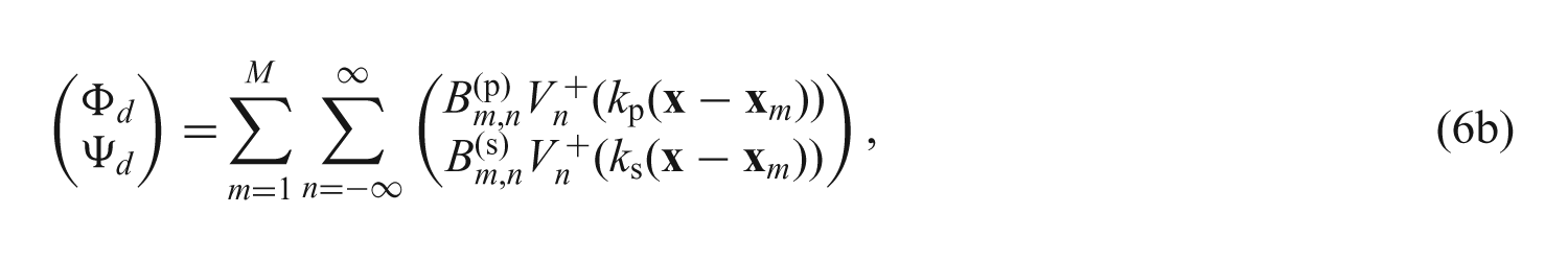
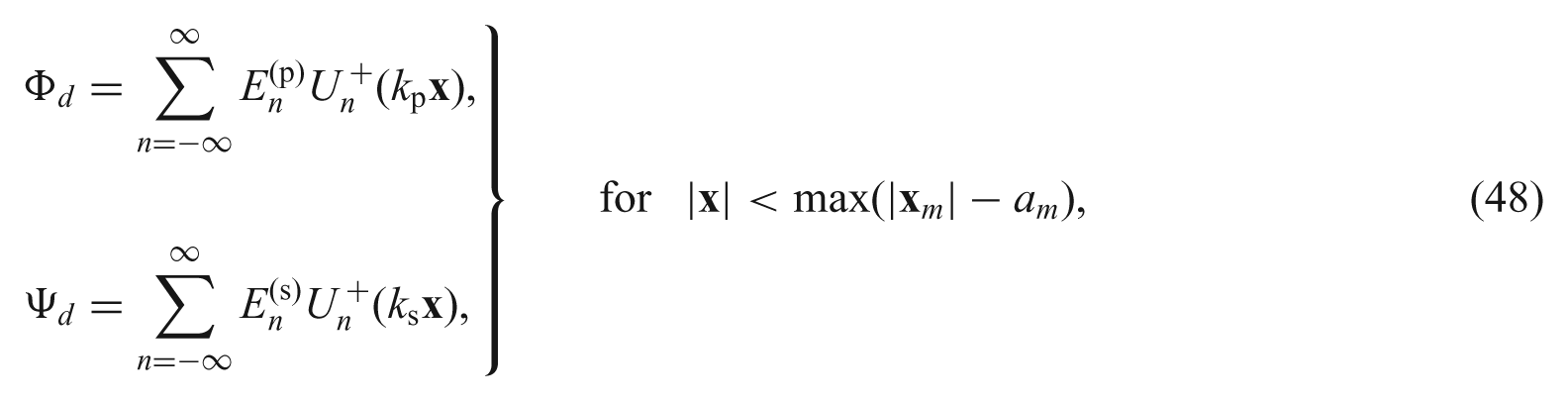
The infinite series associated with the multipole expansion of the mth active source is formally divergent inside the circle that is centered on the source itself, i.e. for |
As yet it does not appear that active exterior cloaking has been applied to the elastodynamic context. This paper will focus on the relevant 2D active elastodynamic cloaking problem. In general, elastodynamic cloaking problems are more difficult to study than their acoustic or electromagnetic counterparts. Indeed in the case of passive elastodynamic cloaking, this is due to the lack of invariance of Navier’s equations under coordinate transformations [16] unless we relax the minor symmetry property of the required elastic modulus tensor. The latter can be achieved by using Cosserat materials [17, 18] or by employing non-linear pre-stress of hyperelastic materials [19–21]. Here we show how the active approach to cloaking can be employed in the elastodynamic case for the fully coupled 2D (in-plane) compressional/shear (P/SV) wave problem. As in the approach of Norris et al. [9] we write down the relevant integral equation by employing, in this case, the isotropic Green’s tensor. The required source amplitudes for arbitrary wave incidence can be determined explicitly by using Graf’s addition theorem.
We shall begin in Section 2 with a statement of the problem, a review of the governing equations, and a summary of the main results. The relevant integral relation is derived in Section 3, from which the main results regarding the explicit form of the source amplitudes are shown to follow. We consider both compressional and transverse (shear) wave incidence. We also describe the form of the active source field and the issues associated with divergence described above. Numerical results follow in Section 4.
2. Problem formulation and main results
2.1 Problem overview
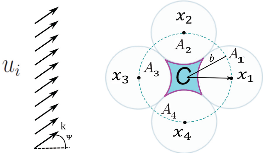
Let us consider the 2D configuration where the active cloaking devices consist of arrays of point multipole sources located at positions
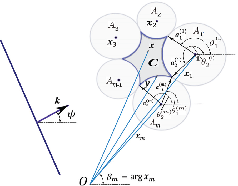
Insonification of the actively cloaked region
The M active sources give rise to a cloaked zone
2.2 Compressional/shear (P/SV) in-plane wave propagation
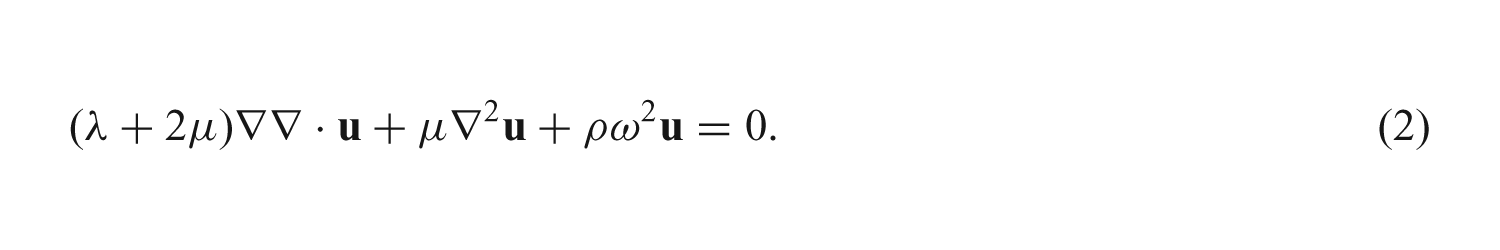
We consider time harmonic solutions with the factor e−iωt understood but omitted. Navier’s equations in 2D for the displacement
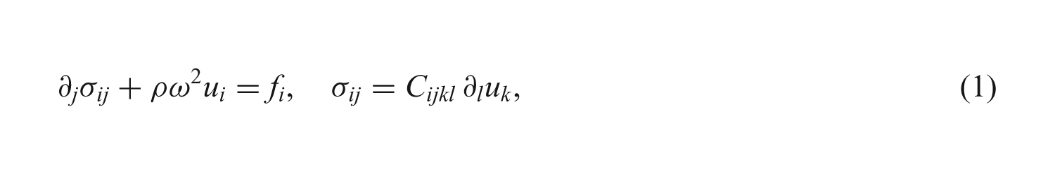
where
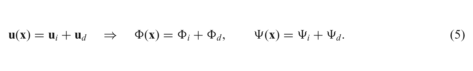
The Helmholtz decomposition for the displacement,
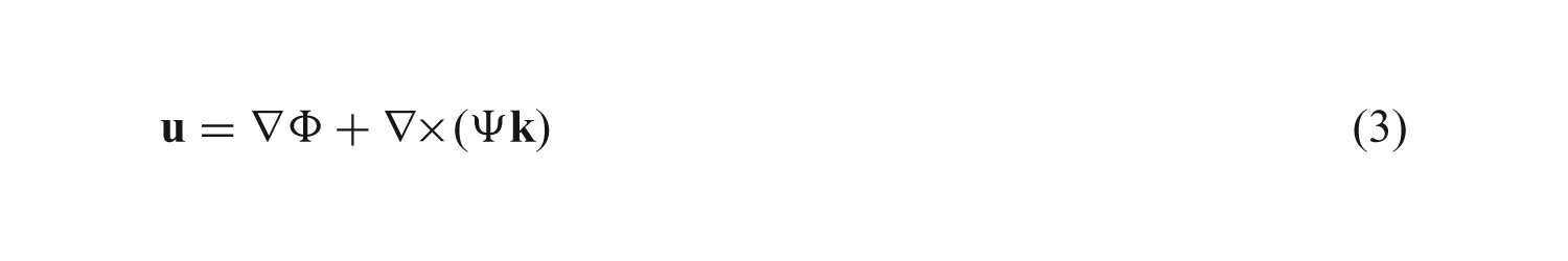
leads to separate Helmholtz equations for the scalar potentials
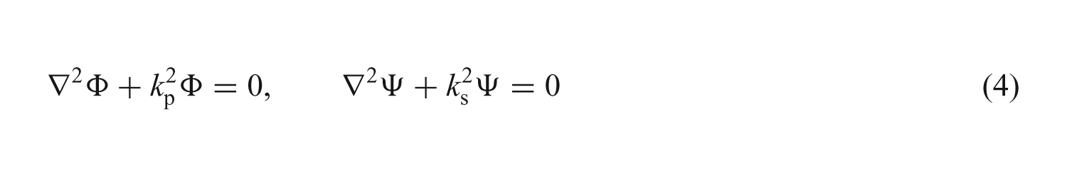
where kp, ks are the longitudinal and shear wave numbers, respectively:
We assume the general form of an incident field in the regular basis, and hence
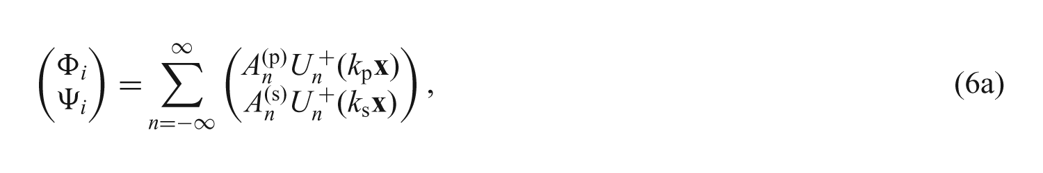
where the functions
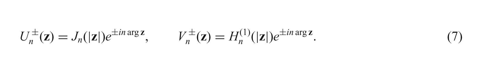
Here arg
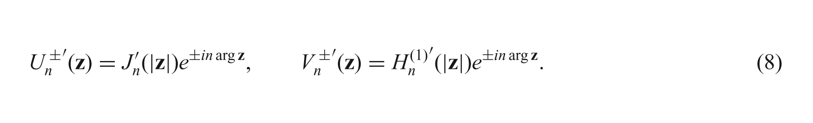
Note that the functions
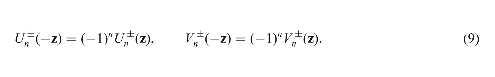
In the following we write U0 and V0, with obvious meaning.
2.3 Summary of the main results
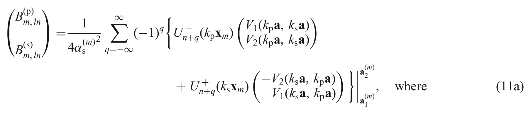
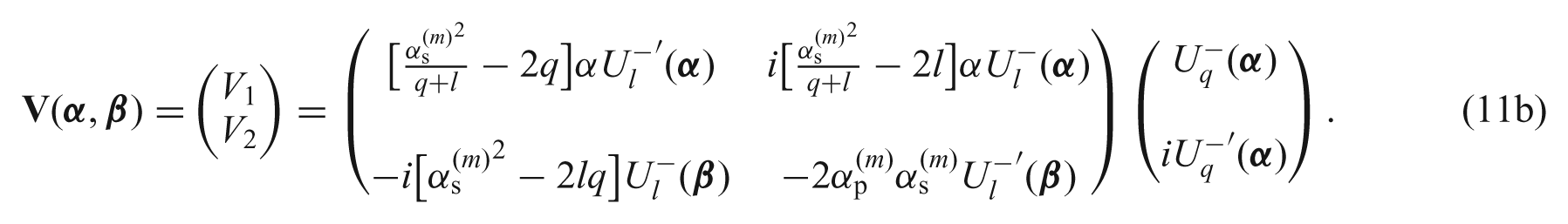
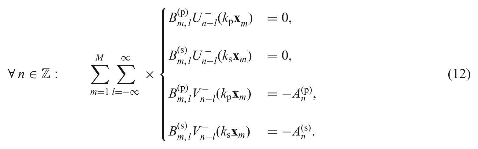
Here we shall state the main results and the required source amplitudes to enable perfect active cloaking together with necessary and sufficient conditions on these amplitudes. The latter ensures we can compare accuracy of the cloaking technique. We shall prove these results in Section 3. Let
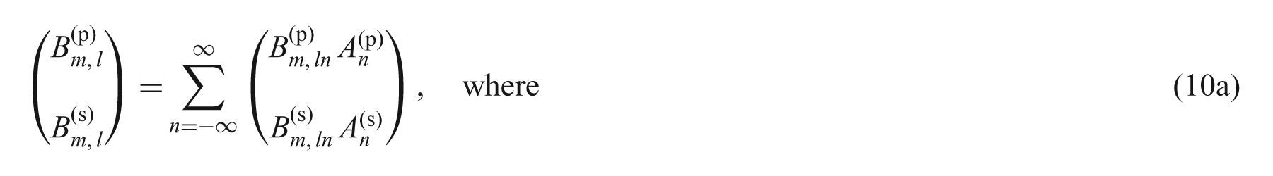
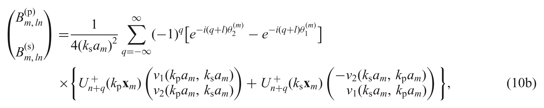
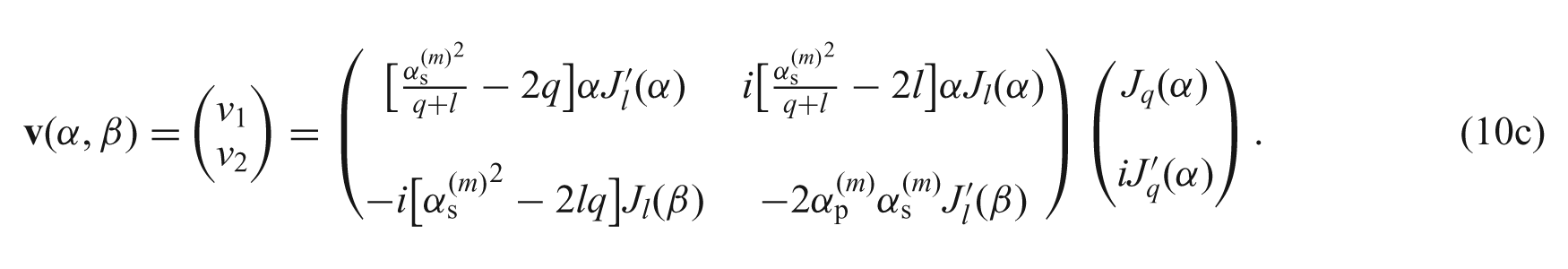
The derivation of equation (10) is given in Section 3.4. Alternatively, defining a vector
Next, we note that the active source coefficients
The first pair of conditions is required to ensure zero radiated field outside the union of the active regions,
3. Derivation of the source amplitude expressions and constraints
Let us first formulate the problem in terms of an integral equation.
3.1 Green’s tensor and integral equation formulation
Consider the particular solution of Navier’s equations (1) in the presence of a point force,
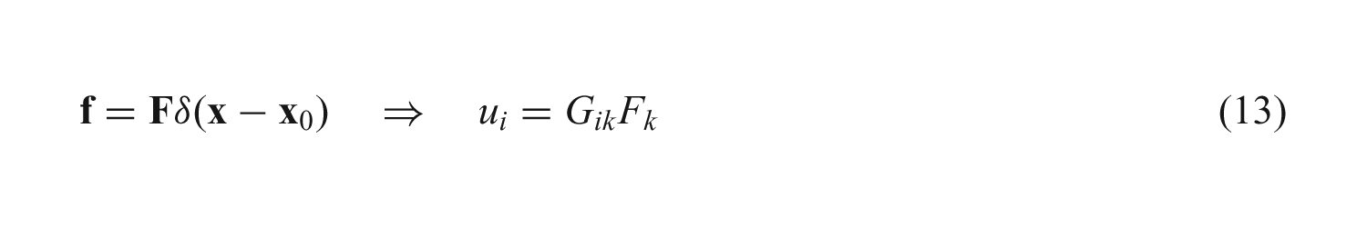
where Gik is the 2D (in-plane) Green’s tensor. Specifically, Gik(
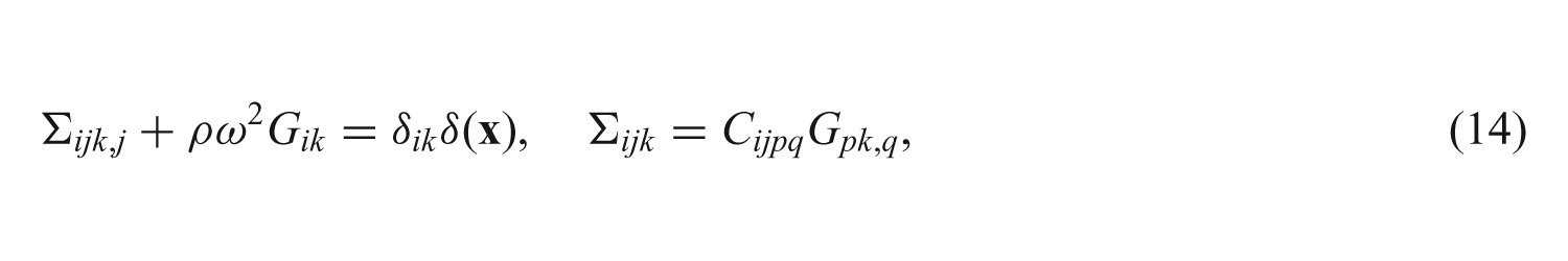
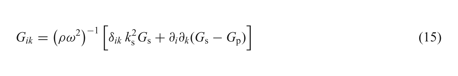
with solution
where
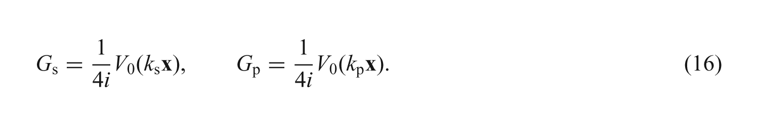
The solution in equation (15) can be checked by substitution into the governing equation (14) and using the identities
It is convenient to work without subscripts, writing equation (15) as
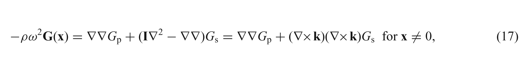
where (∇×

implying
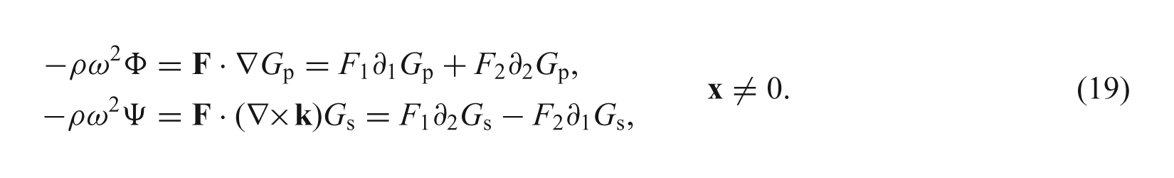
This makes it clear that for a standard point source, regardless of the choice of
With knowledge of Green’s tensor we can now develop an integral equation for the displacement. Indeed, if
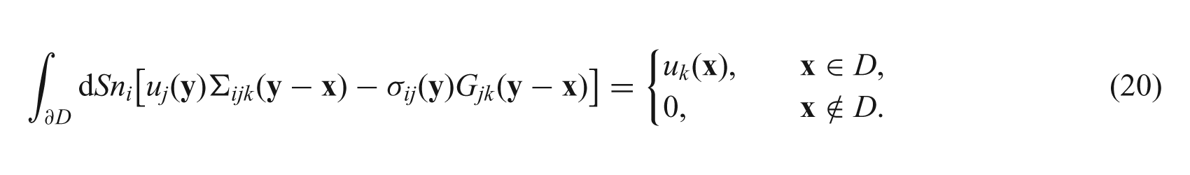
Equation (20) holds for both
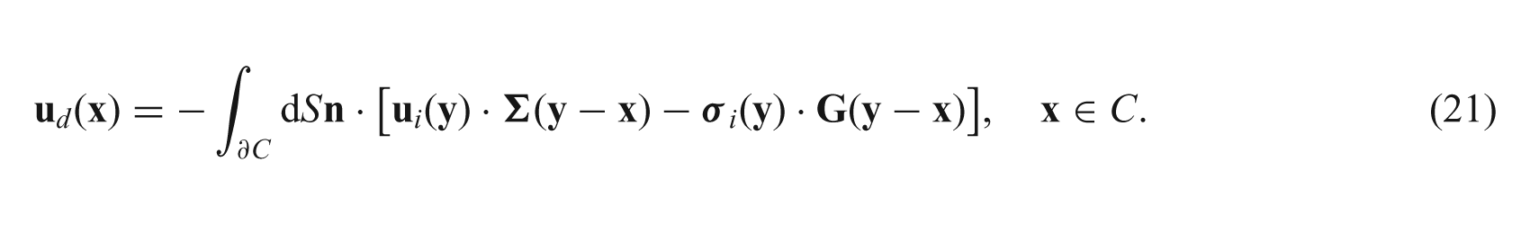
This is the fundamental relation used to find the source amplitudes.
3.2 General expressions for the source amplitudes
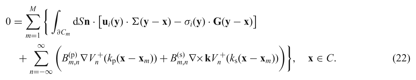
Following the procedure for the Helmholtz problem [9], we first substitute the assumed form of
We now use the generalized Graf addition theorem [22, equation (9.1.79)],
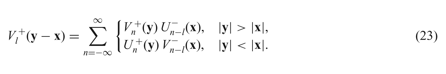
The idea is to write Σ(
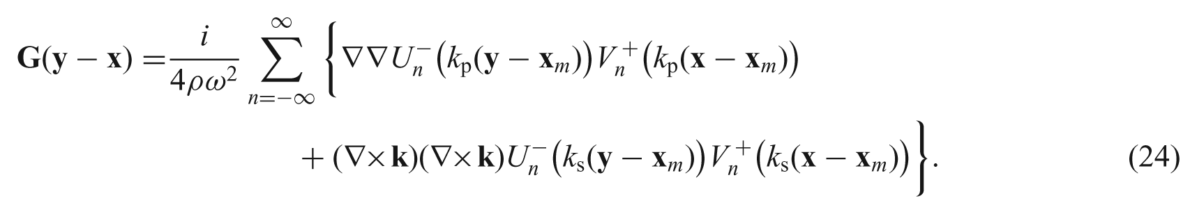
By virtue of the dependence of Green’s function on
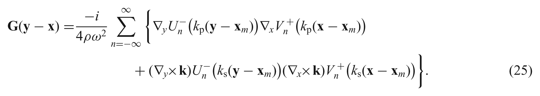
Substituting from equation (25) into equation (22), and identifying the coefficients of
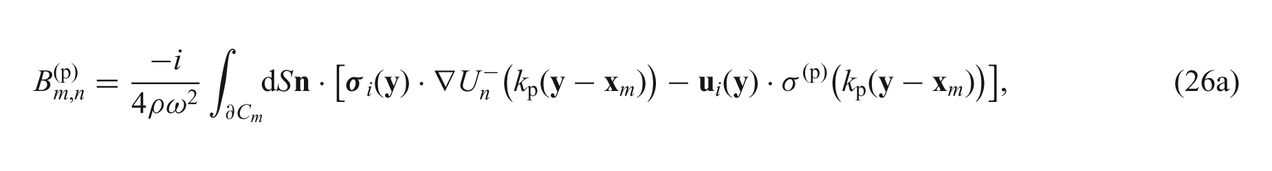
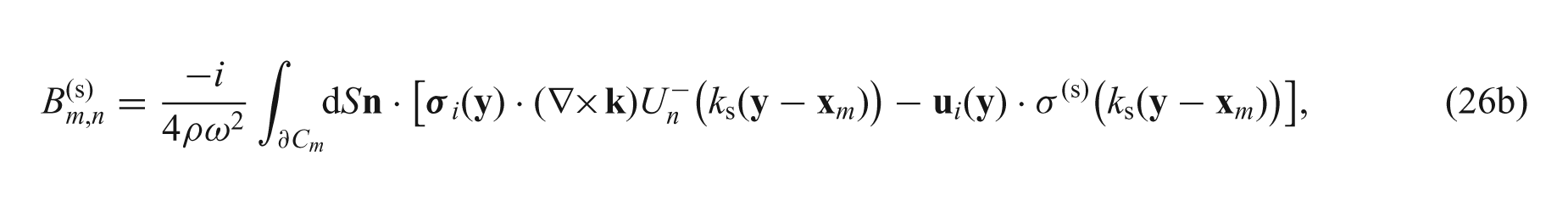
where
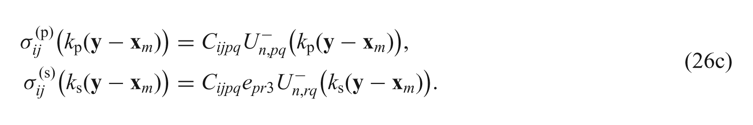
Therefore, given the incident field, we are now able to evaluate the required source amplitudes that guarantee zero total field inside the domain

The four distinct terms in the integrals of equation (26), such as
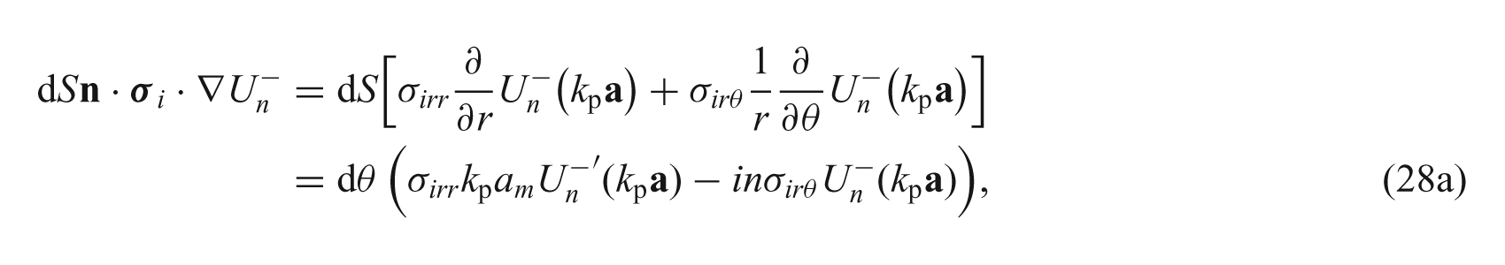
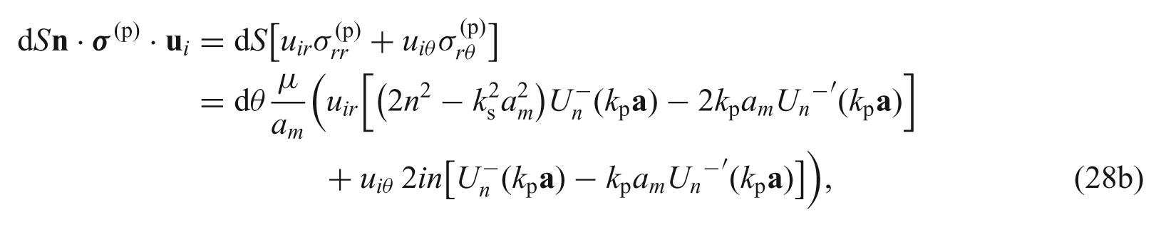
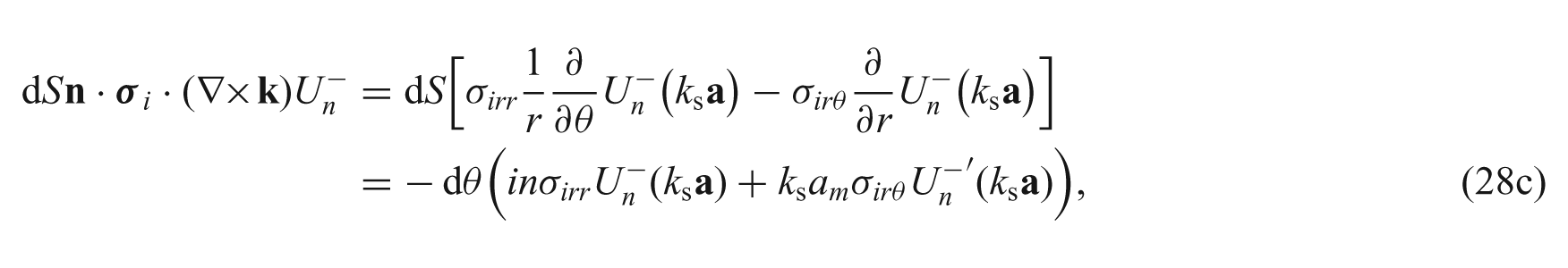
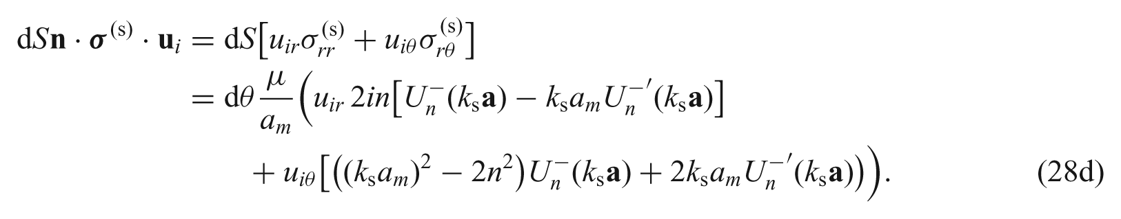
Noting the reversal of the sense of the integral in equation (26) and incorporating equation (28a) leads to
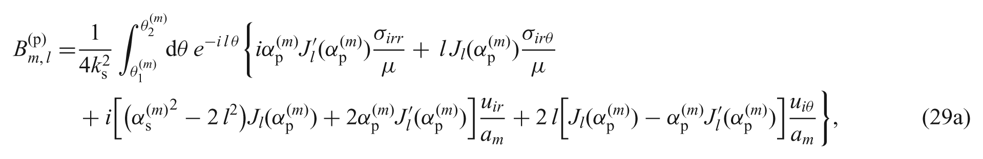
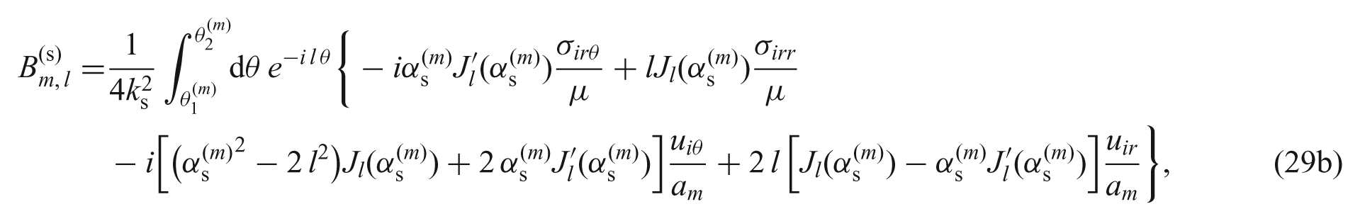
where
Let us now specialize the result to the specific case of plane wave incidence. This is important in its own right but also allows us to derive the general incident wave case by integration as we shall show.
3.3 Plane wave incidence
Let us define
where
3.3.1 Longitudinal incident plane wave
Consider now longitudinal plane wave incidence
where Ap ≡ const is a known wave amplitude. Then using the relation Φ
i
(
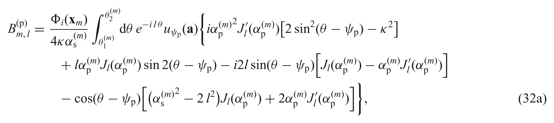
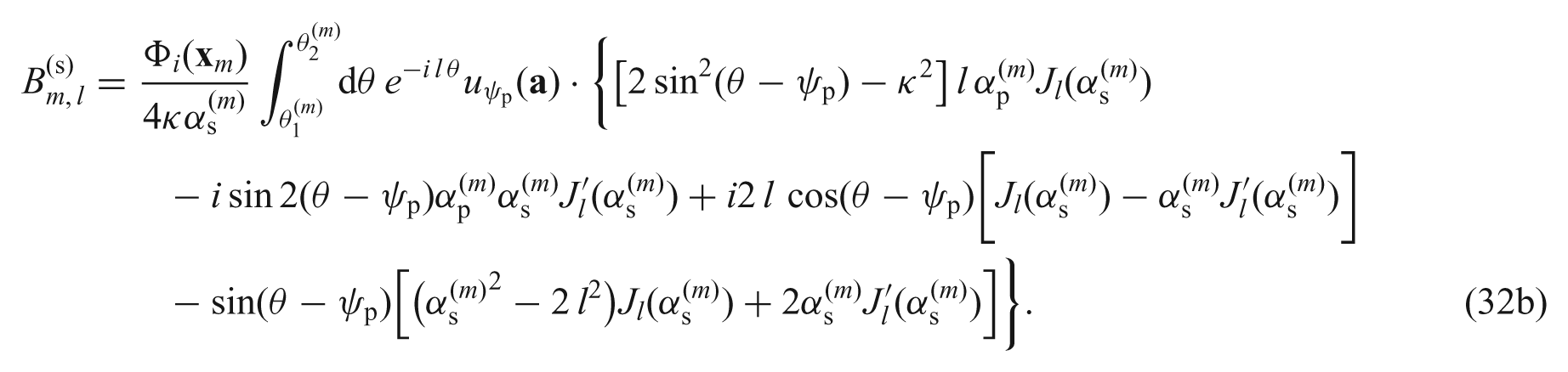
Then noting that uψp(
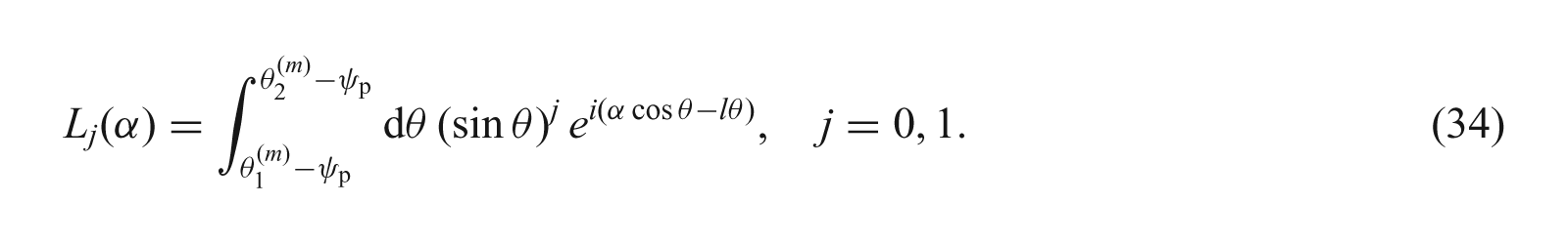
where the functions L0(α) and L1(α) are defined by
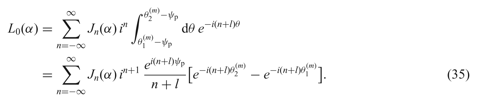
L0(α) can be evaluated by using the Jacobi–Anger identity
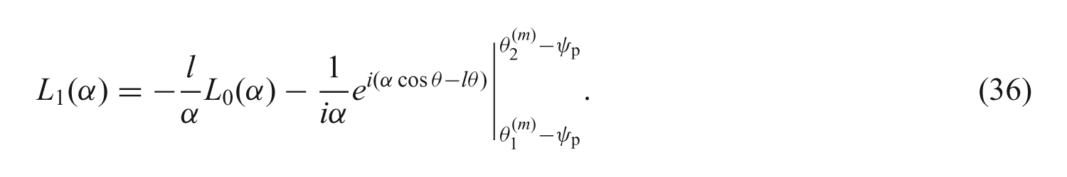
Integration by parts yields L1(α) in the form
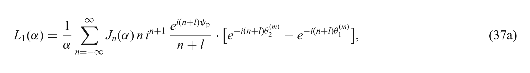
Taking into account the Jacobi–Anger identity and equation (35), the function L1(α) and its derivative L1 ′ (α) can be expressed
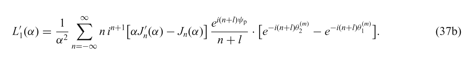
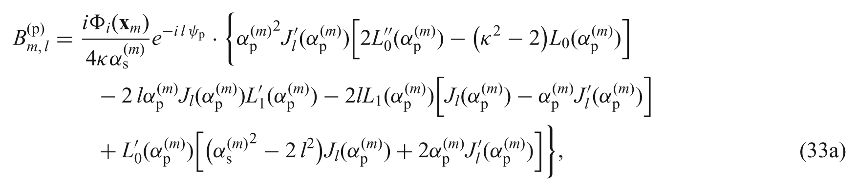
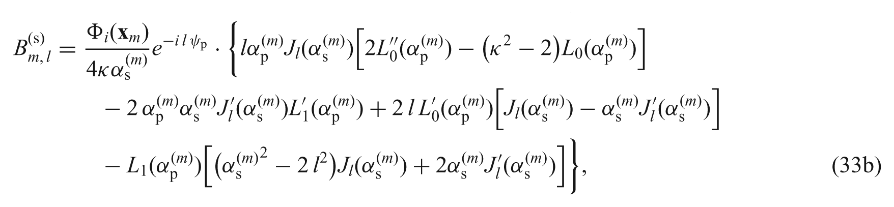
Introducing the explicit results for the functions L0(α) and L1(α) into equation (33) yields expressions for the amplitude coefficients in the form:
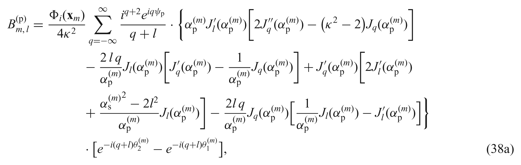
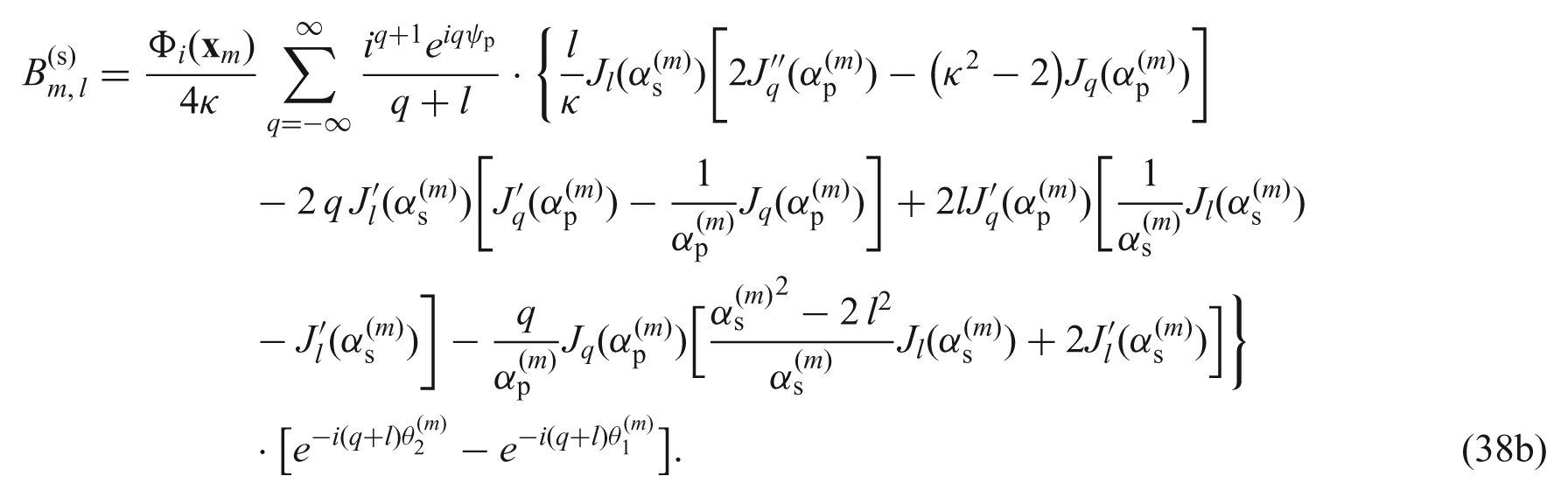
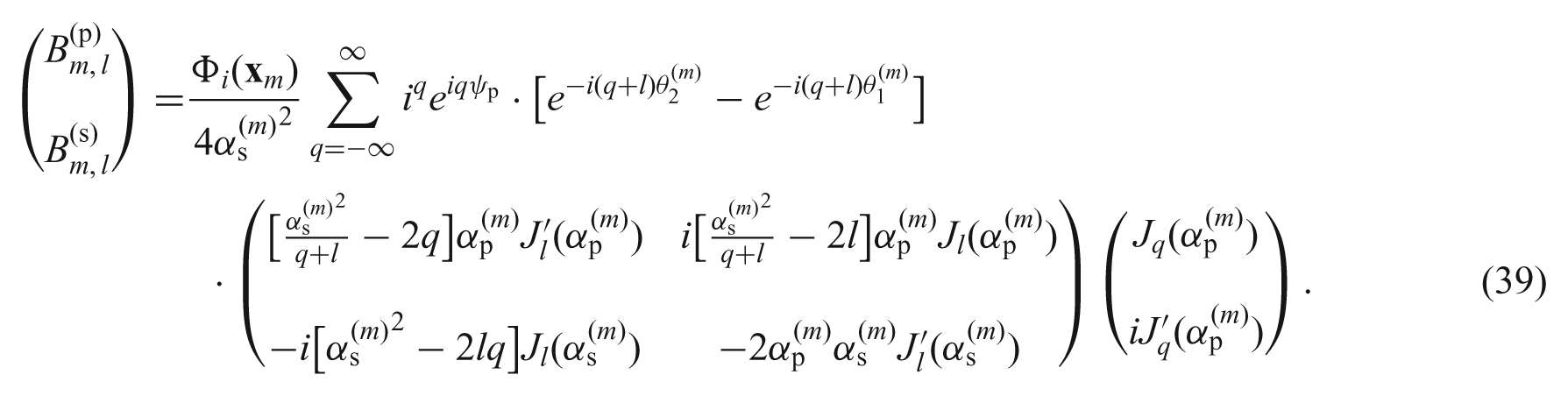
After some simplification equation (38) can be written as
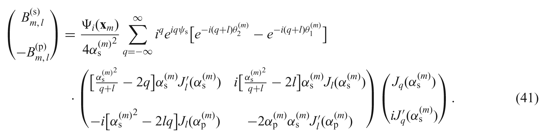
3.3.2 Transverse plane wave incidence. Consider now an incident transverse plane wave
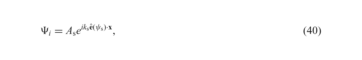
where As ≡ const is a known transverse wave amplitude. Entirely analogous calculations to the compressional wave case yield the source amplitudes in the form
3.3.3. Plane wave incidence summarized
Adding the separate results of equations (39) and (41) gives for combined incidence
the source amplitudes
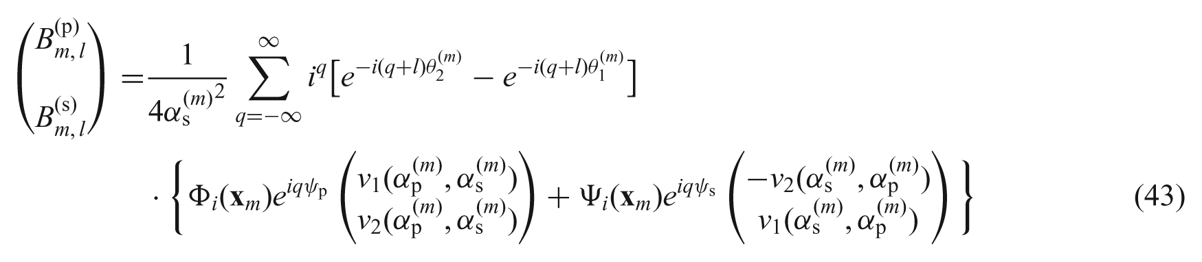
where the vector
3.4. Arbitrary incident field as superposition of plane incident waves
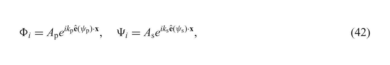
The general form of incident field given by equation (6a) can be constructed as a superposition of plane incident waves of the form of equation (42). This will enable us to find the general form of the amplitude coefficients for incident waves of general form as a superposition of solutions for plane waves given by equation (43). Recall the incident field for a combined incident plane wave having the form
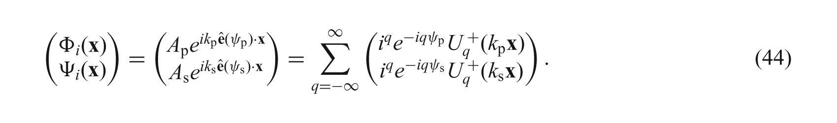
Multiplying the first row of equation (44) by (i−(n+q)/2π)ei(n+q)ψp and the second row by (i−(n+q)/2π)ei(n+q)ψs, integrating with respect to ψp and ψs respectively between 0 and 2π and then evaluating at
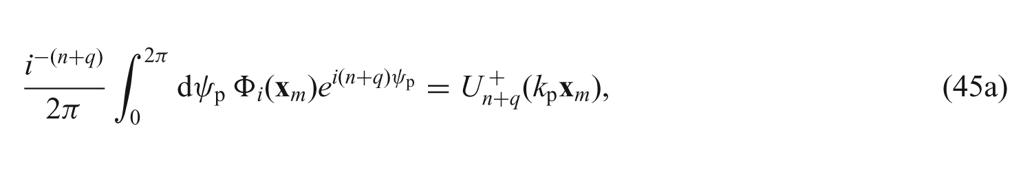
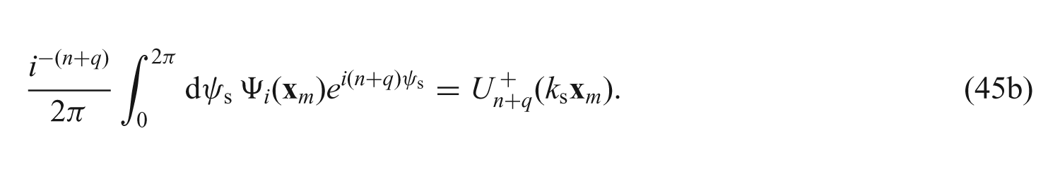
To obtain the form of the amplitude coefficients given by equation (10) for the general incidence in equation (6a) we multiply the first and second of the equations in equation (43) by
3.5. Necessary and sufficient conditions on the source amplitudes
In this section we will define the constraints on the active source coefficients
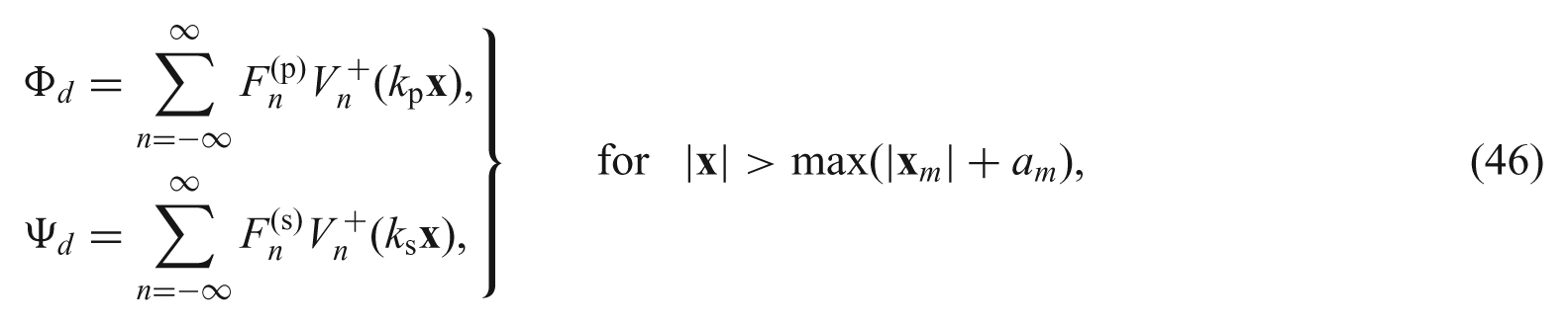
where

If the active field Φd and Ψd does not radiate into the far-field, then we must have
Next we consider the near-field. Assuming |
where
If the total field is zero in the near-field, then we must have
3.6 Divergence of the active field summation
The infinite sum expression for the active source fields defined by equation (6b) with source amplitudes (10a)–(10c) is formally valid only in |
Active cloaking therefore requires that we use the expression in equation (6b) with source amplitudes (10a)–(10c) for the active field everywhere but we must take a finite number of terms in the multipole expansion. That is, we use the source amplitudes that appear in the infinite sum as motivation for the choice of source amplitudes that should be chosen in an active field that contains only a finite number of multipoles. This ensures a finite (but large) field inside
With a finite sum for the active field therefore, the integral equation (20) is not perfectly satisfied but instead

and the field is large (but finite) inside
4. Numerical examples
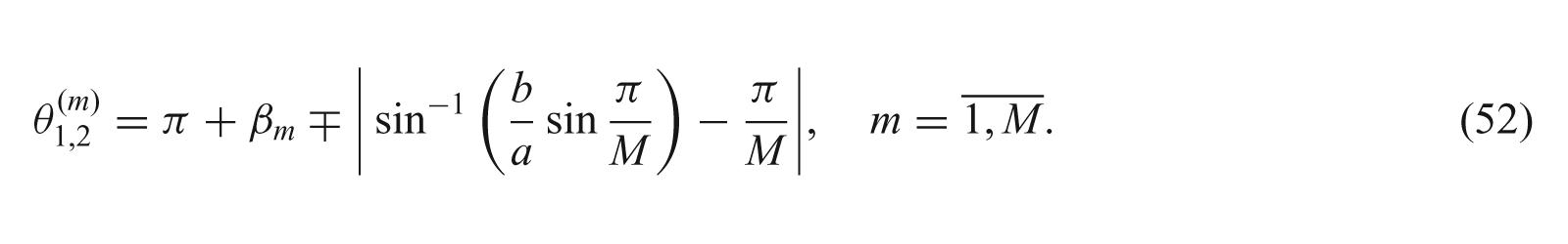
The numerical calculations for active source configurations of the type shown in Figure 2 are performed for plane longitudinal and transverse incident waves of a unit amplitude, (Ap = 1, As = 0) and (Ap = 0, As = 1), for angles of incidence ψp =ψ s = 7°. Variable values are taken for the wave numbers kp and ks, the number of sources M, and the number of terms N in equations (47) and (49) (the truncation size). The M active sources are symmetrically located on a circle of radius b, with
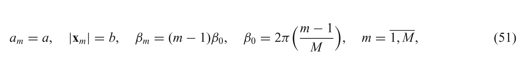
where βm is the argument of vector
Plane wave insonification of the cloaking region
In all examples, we take
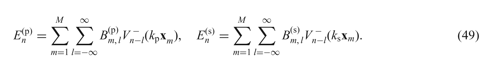
4.1. The scattering amplitudes
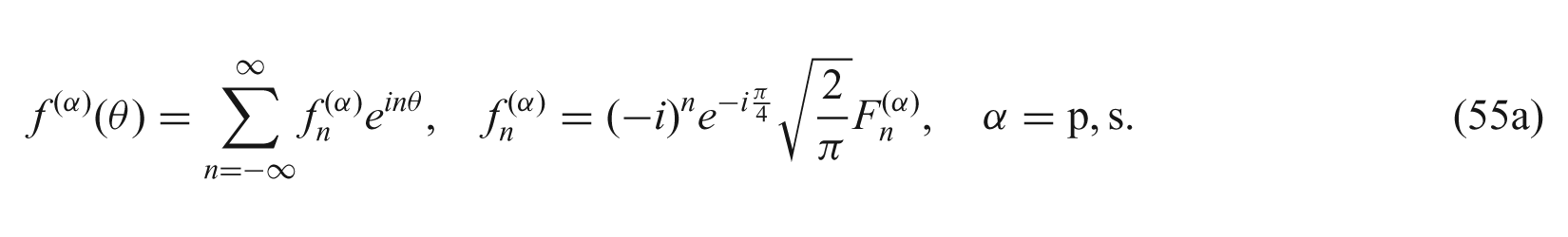
Consider the truncated versions of the infinite sums in equation (49) for the far-field amplitudes
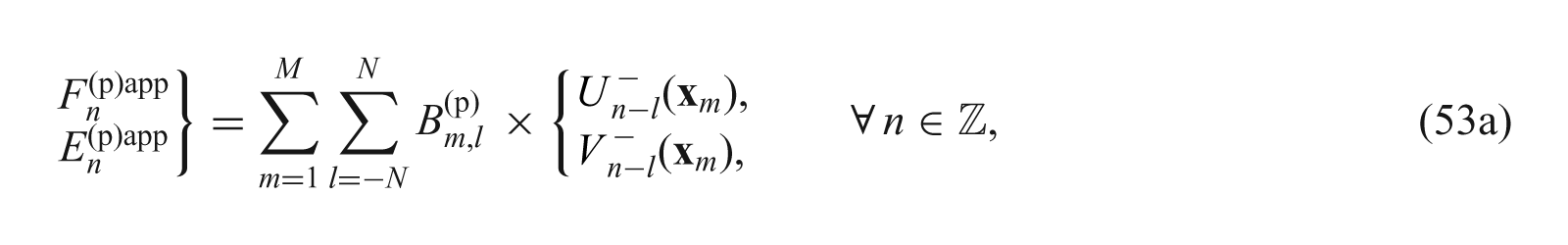
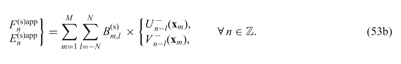
The approximate near-field
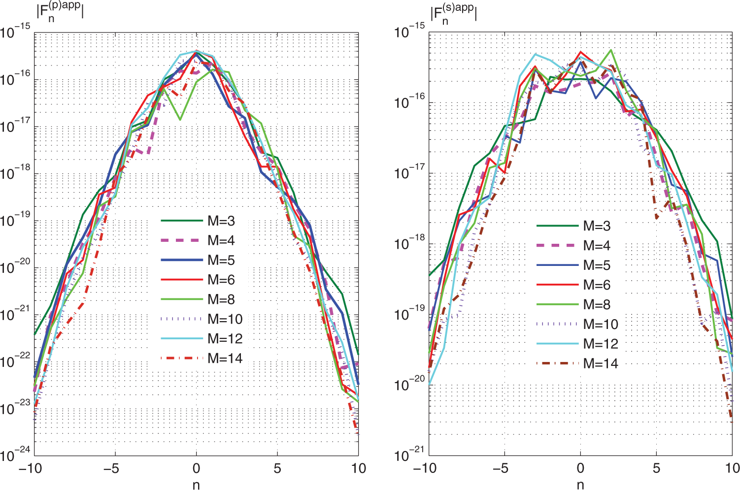
Variation of the far-field amplitude coefficients with number of active sources
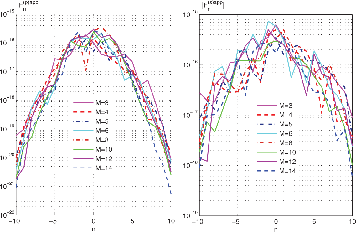
Variation of the far-field amplitude coefficients with number of active sources
The variation of the near-field coefficients
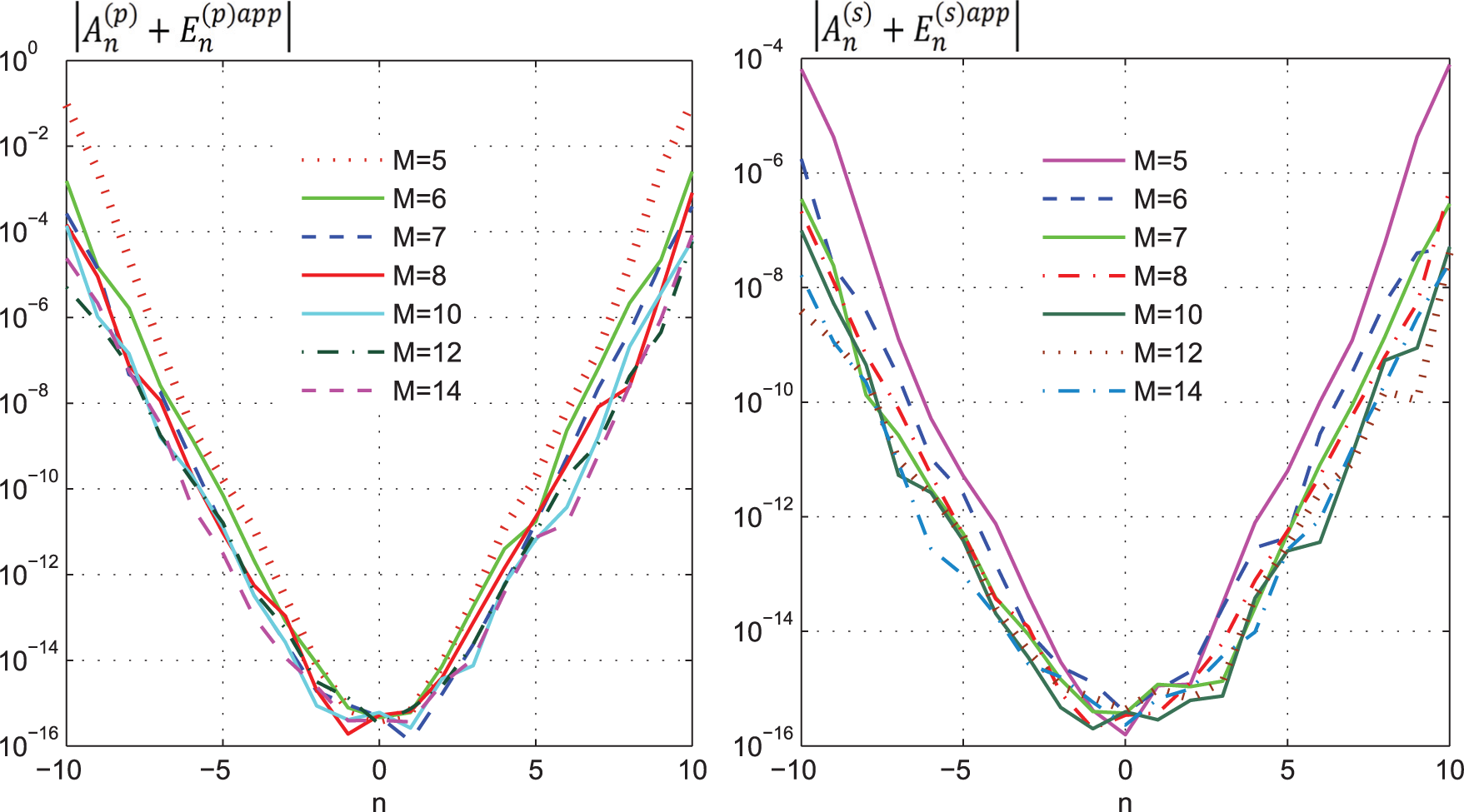
Dependence of the near-field amplitude coefficients on n, the order of Bessel function, varying the number of active sources
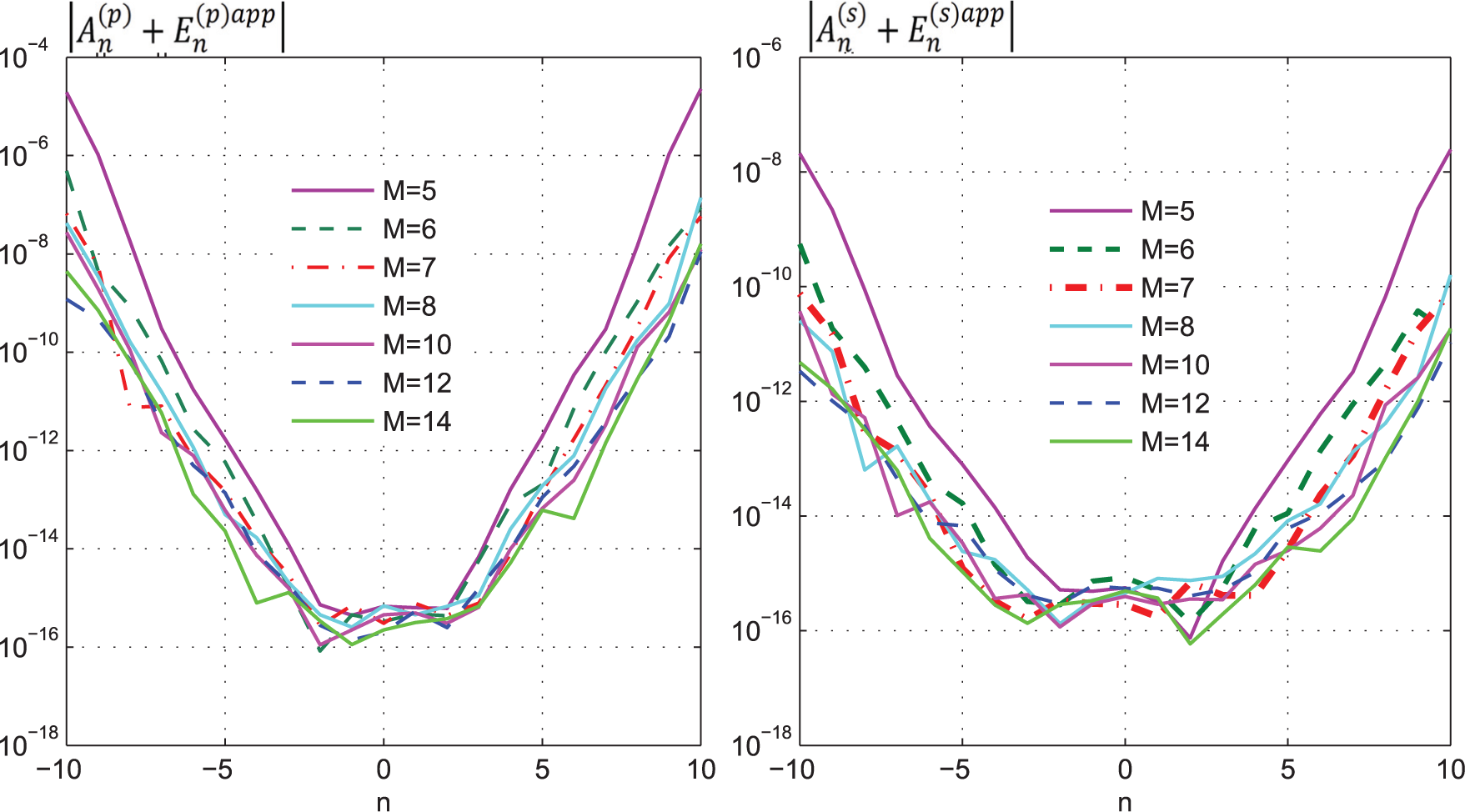
Variation of the near-field amplitude coefficients with number of active sources
Figure 7 displays the near-field amplitude coefficients
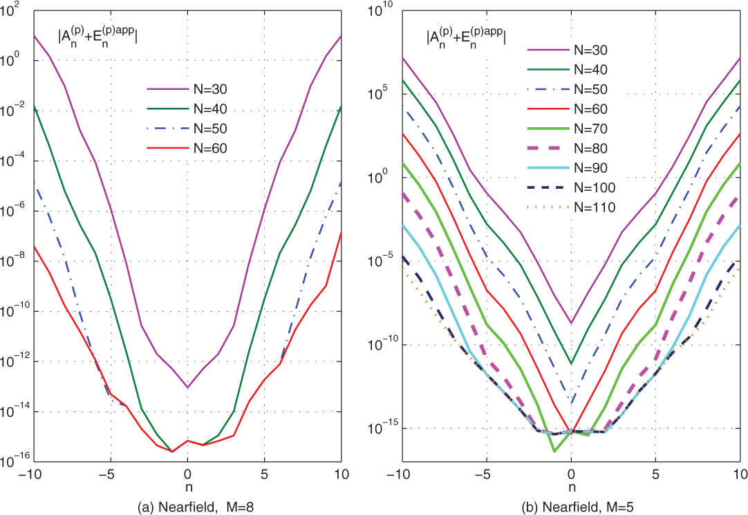
The near-field amplitude coefficients as a function of the Bessel function order n for different values of the truncation size N in equation (53) generated by (a) M = 5 and (b) M = 8 active sources, for longitudinal incidence.
4.2. Far-field response
The radiated field as
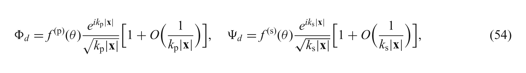
where f(p) and f(s) are the far-field amplitude functions,
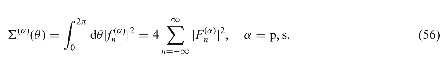
The total power radiated by the sources is Σ(θ) =Σ (p)(θ) +Σ (s)(θ) where the compressional and shear far-field averaged radial flux vector components are
The non-dimensional total scattering cross sections are then
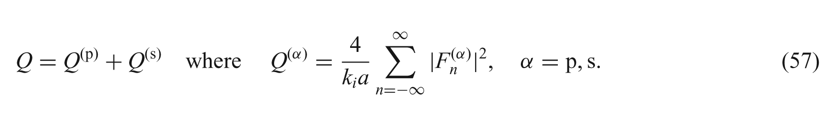
and ki = kp for compressional incidence, ki = ks for shear wave incidence. Q(p) and Q(s) are normalized by a = a1, the radius of source A1, see Figure 1.
Results for the total scattering cross sections Q(p) and Q(s) for both longitudinal and transverse incidence are illustrated in Figure 8 versus the normalized wave number kia, and in Figure 9 against the number of active sources M. These show that the error increases with the rise of wave number ki, but can be reduced by increasing M and N. The increase of N reduces the error sharply in all cases.
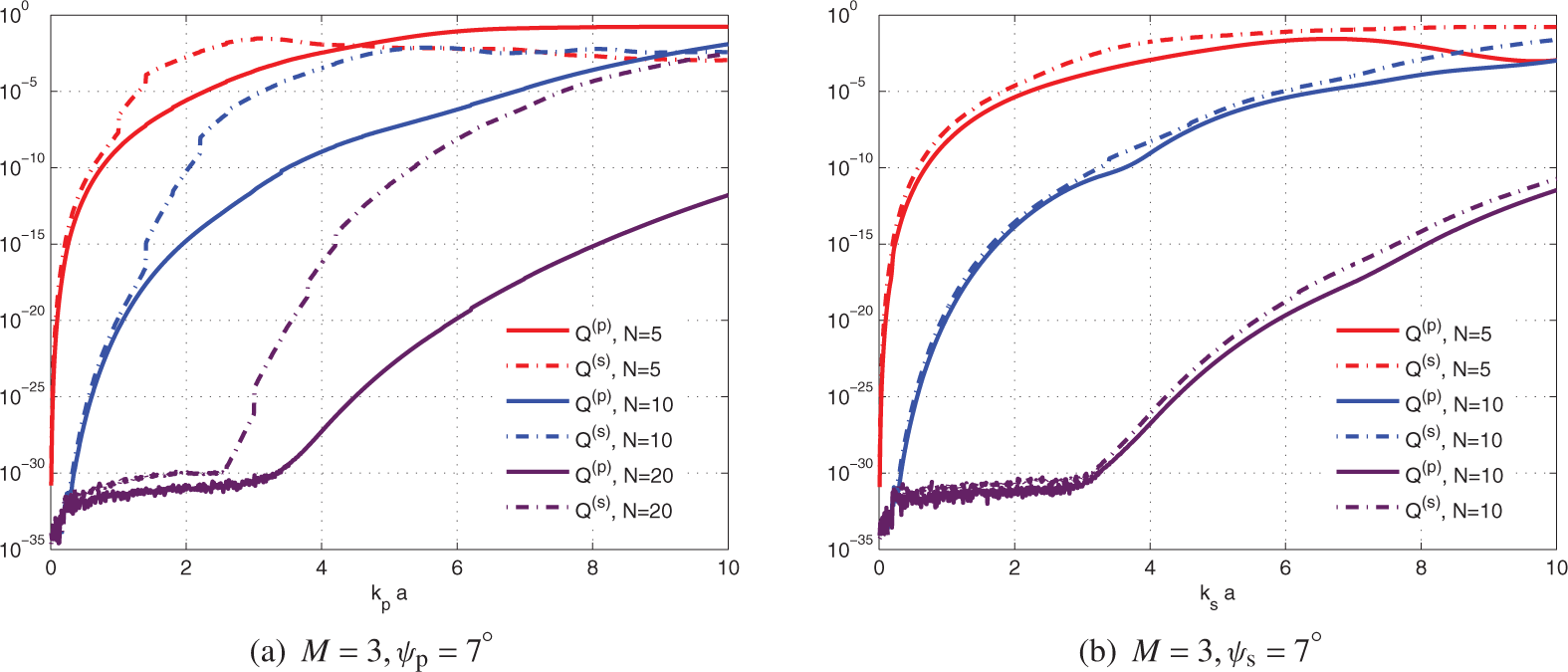
The total scattering cross sections Q(p) and Q(s) versus (a) the normalized wave number kpa for a longitudinal wave incidence, and (b) ksa for a transverse incidence.
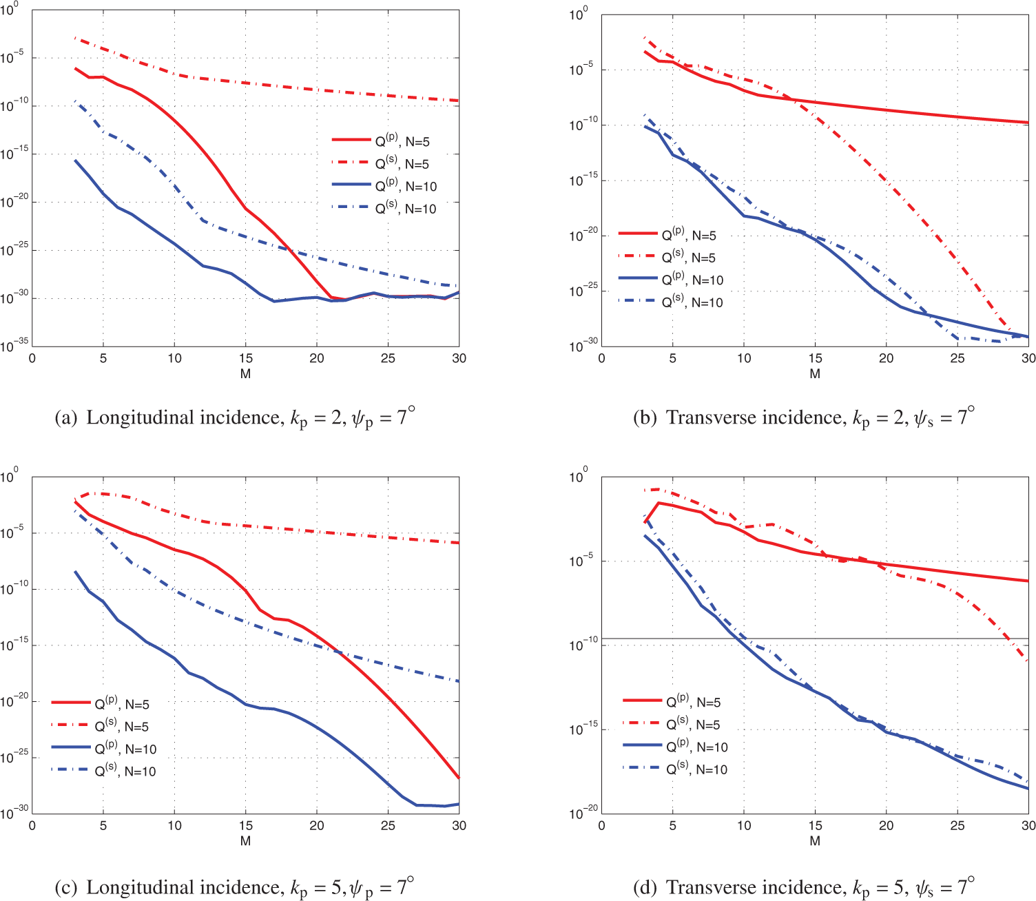
Total scattering cross sections Q(p) and Q(s) versus the number of active sources M for longitudinal ((a) and (c)), and transverse ((b) and (d)) wave incidence for kp = 2 and kp = 5 with ks =κ kp and κ = cp/cs when cloaking devices are ON.
4.3. Total displacement field
4.3.1. Longitudinal plane wave incidence
First, consider longitudinal plane wave incidence of the form of equation (31). The total displacement vector components in Cartesian coordinates are
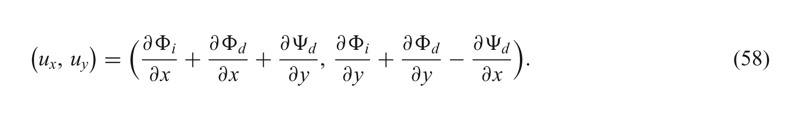
Introducing equations (31) and (6b) into equation (58) yields
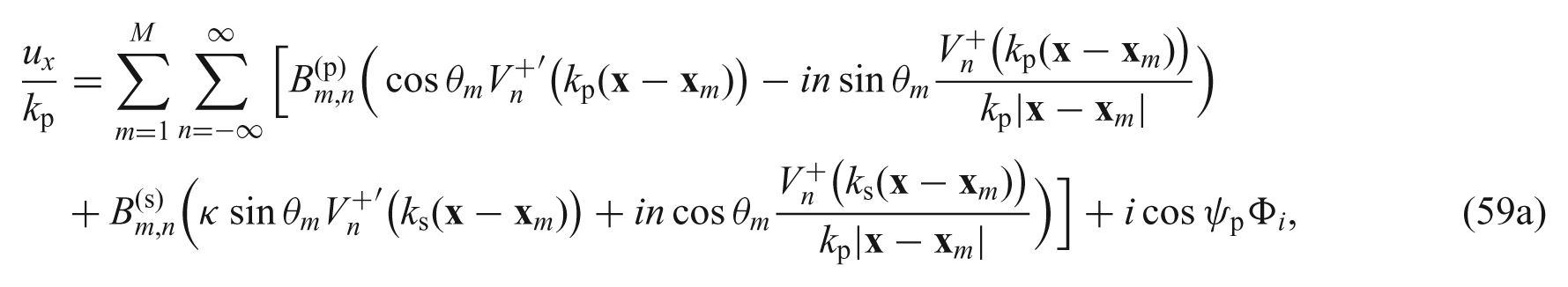
where
4.3.2. Transverse plane wave incidence
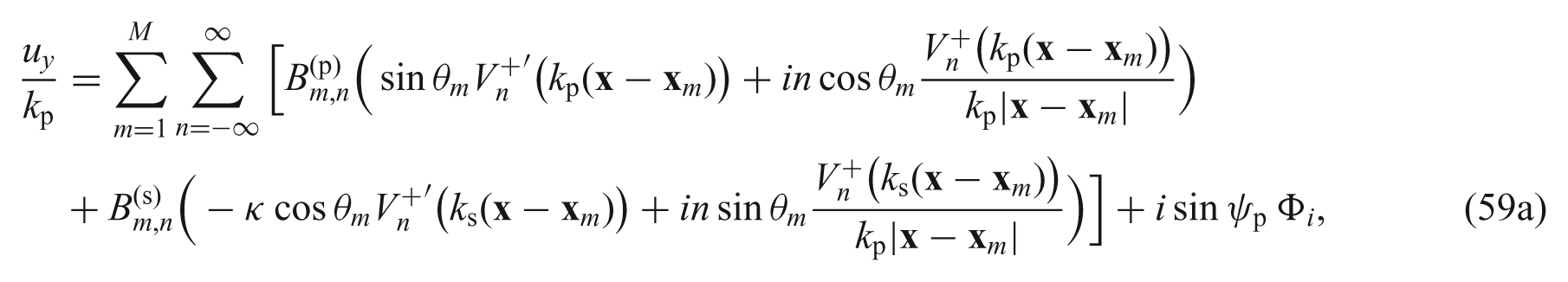
Transverse incident plane waves are of the form of equation (40). The total displacement vector components in Cartesian coordinates are
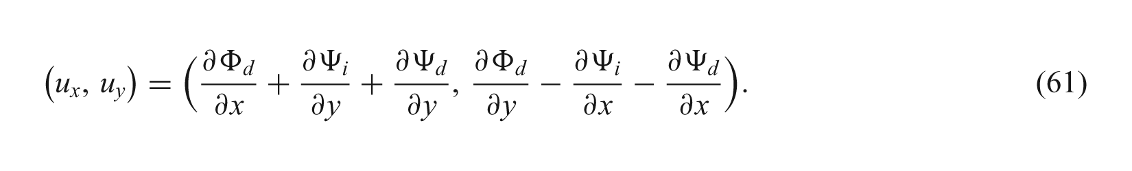
Introducing equations (40) and (6b) into equation (61) yields
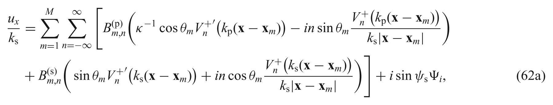
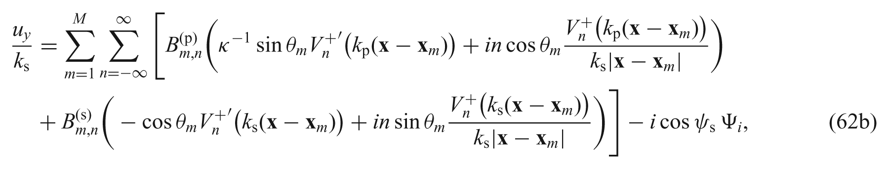
where θm is defined by equation (60).
4.3.3. Results
The magnitude of the displacement vector components ux and uy are evaluated for ψp = 7° for various values of the truncation size N, the number of sources M, and the compressional wave number kp. Greater accuracy is observed, as expected, with increased N and M. However, large N and M require longer computation time, and some numerical experimentation is necessary to find the smallest values for which the displacement field vanishes to the desired degree in the cloaked region.
The magnitudes of |ux|/kp and |uy|/kp are depicted in Figure 10 and Figure 11 for longitudinal incidence at different values of N when cloaking devices are active with M = 3, kp = 2. As expected, the increase of N is accompanied by the reduction of magnitudes |ux|/kp and |uy|/kp in the cloaked region.
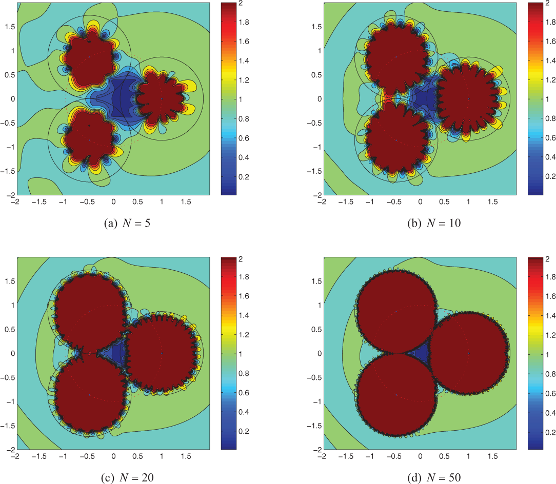
Absolute value of the displacement vector component |ux|/kp for N = 5 (a), N = 10 (b), N = 20 (c) and N = 50 (d) when cloaking devices are active with M = 3, kp = 2 for longitudinal wave incidence.
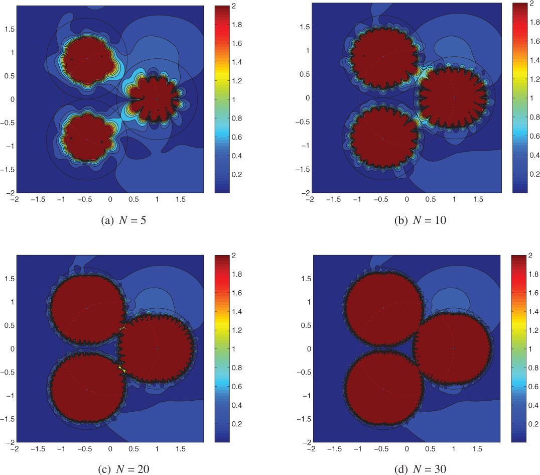
Absolute value of the displacement vector components |uy|/kp for N = 5 (a), N = 10 (b), N = 20 (c) and N = 30 (d) when cloaking devices are active with M = 3, kp = 2 for longitudinal wave incidence.
Figure 12 illustrates |uy|/kp for longitudinal incidence with N = 5 changing the values of kp and M whilst Figure 13 and Figure 14 show corresponding values of |ux|/ks and |uy|/ks for shear incidence, varying N and M with kp = 2 for the former, and altering the values of N and kp with M = 3 for the latter. The magnitude of the total displacement field and its absolute maximum amplitude inside the cloaked region is depicted in Figure 15 with the parameters used in Figure 12. Comparison of these results shows that at higher frequencies, i.e., larger values of kp, greater accuracy is achieved by increasing the number of sources M, whereas at lower frequencies the smallest number of sources required, i.e. M = 3, produces reasonable cloaking, although this is enhanced with increased values of N.
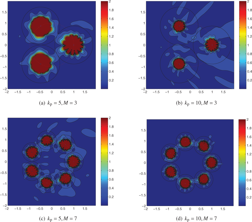
Absolute value of the displacement vector component |uy|/kp for kp = 10, M = 3 (a), kp = 10, M = 3 (b), kp = 5,M = 7 (c) and kp = 10,M = 7 (d). Cloaking devices are active, N = 5, and longitudinal wave incidence.
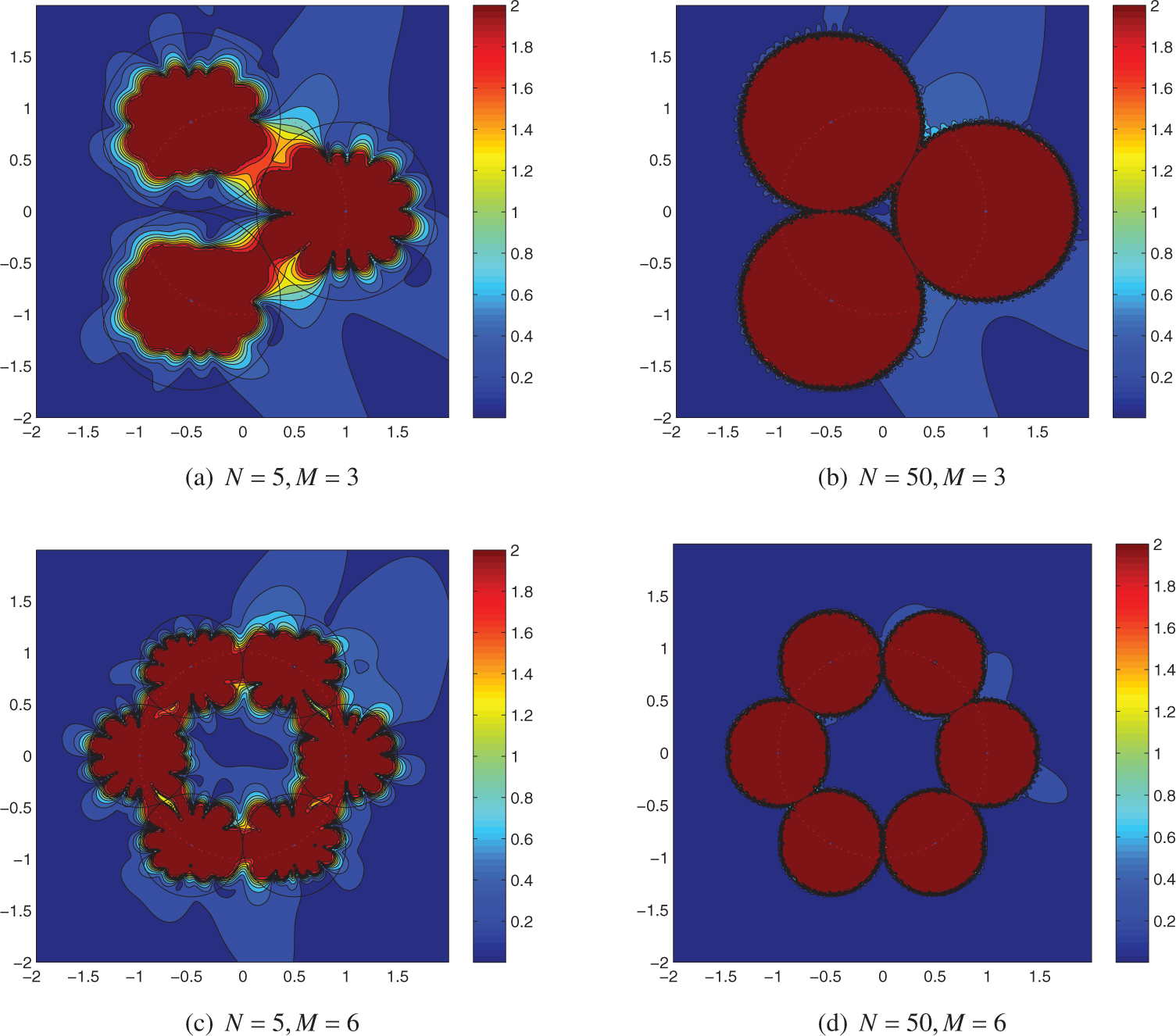
Absolute value of the displacement vector component |ux|/ks for N = 5, M = 3 (a), N = 50, M = 3 (b), N = 5, M = 6 (c) and N = 50, M = 6 (d) when cloaking devices are active with kp = 2,ks = 4.1305 for transverse wave incidence.
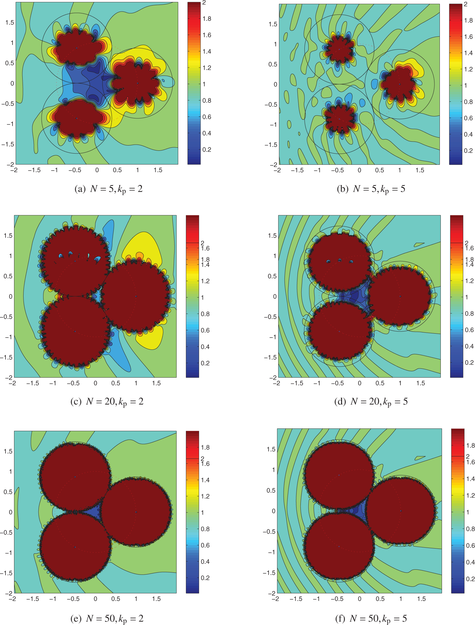
Absolute value of the displacement vector components |uy|/ks for N = 5, kp = 2 (a), N = 5, kp = 5 (b), N = 20, kp = 2 (c), N = 20, kp = 5 (d), N = 50, kp = 2 (f), and N = 50, kp = 5 (e) with M = 3 active sources for transverse wave incidence when the cloaking devices are active.
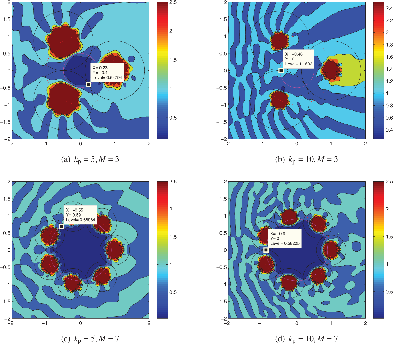
The magnitude of the total displacement field with its maximum absolute amplitude in a cloaked region generated by M = 3 active sources with kp = 5 (a) and kp = 10 (b), and by M = 7 active sources with kp = 5 (c) and kp = 10 (d) for a longitudinal wave incidence with ψp = 7°, N = 5 while cloaking devices are active.
5. Conclusions
The external active acoustic cloaking model of Norris et al. [9] has been generalized to elastodynamics. Just as in the former case, it is possible to represent the sources in exact terms, although it requires that the incident elastic wave field is known in exact form; this is the price paid for active control. The control method proposed is based on representing the incident field in terms of regular functions (Bessel functions) at each source position, which leads to a linear system of equations for the source amplitudes that can be solved in closed form. The linear nature of the solution of this essentially inverse problem means that arbitrary incident wave motion can be treated by superposition.
The results presented here provide a first step in the direction of realistic active control of elastic waves. Applications to structure borne waves, surface waves, and even geophysical waves, are possible. However, as a control problem, many issues remain to be addressed. Not least is the issue of how to balance the goal of silencing one region of space with the unavoidable source noise that must be generated in another, larger, region. This quandary arises from the fact that the infinite series for the multipole expansion of the m active sources is divergent inside the domain Am. Exact field cancellation is not achievable in practice; it becomes necessary to truncate the series and balance the decrease in cloaking accuracy with whatever amplitude level is deemed acceptable in the source region. This is obviously a crucial aspect and one that remains to be studied in detail. We have pointed out some similarities with parallel issues in active noise control, and future studies will examine analogies in these topics. One area for consideration is the low-frequency end of the spectrum. The numerical simulations presented here indicate that a small number of multipoles provide adequate cancellation at low frequencies. This suggests a natural way to extend ideas based on monopoles to more elaborate source distributions composed of finite numbers of multipoles of low order. Hopefully, the present results provide a means to establish realistic strategies for practical application.
Footnotes
Funding
This work was supported by the ONR and the NSF.
Conflict of interest
None declared.