On the equations of motion for curved slender beams using tubular coordinates

Abstract

The equations of motion for a beam are derived from the three-dimensional continuum mechanical point of view. The kinematics involve bending, torsion and shearing as well as cross-sectional displacements. The transplacement of the beam from an arbitrary curved reference placement is considered. For slender beams so called tubular coordinates may be used as global coordinates in the reference placement. An explicit geometrical characterization of slender beams is given. The equations of motion for the slender beam are derived and some consequences of the power theorem are presented. Using the principle of virtual power the classical local beam equations are obtained along with equations representing the local balance of bi-momentum. Constitutive assumptions are introduced where the dependence of stress on the natural deformation measures for the beam is obtained by assuming that the beam consists of a St Venant-Kirchhoff elastic material. Simplified stress-strain relations may be obtained using so called torsion free coordinates.

Keywords

Beam theory principle of virtual power equations of motion cross-sectional displacements bi-momentum finite strains

1. Introduction

Beam theory is a highly cultivated area in mechanics. Static theory involving large deflections goes back to James Bernoulli in 1692 and Leonard Euler in 1744 in their treatment of the elastica. This theory is based on the assumptions of pure bending and small strains. Early beam theories are discussed in Ericksen and Truesdell [1]. The Kirchhoff-Love beam model [2] involves shearing as well as bending. It is however still based on a small strain constitutive theory. Reissner [3] developed a theory for plane static problems including finite strain deformations. A fully three-dimensional version, based on director theory, was formulated in Antman [4]. In a series of papers, Simo [5] and Simo and Vu-Quoc [6, 7], a geometrically exact model for beams in motion is presented as well as methods for their finite element implementation. This model is based on kinematics in which the transplacement of the beam cross-sections are rigid. A similar approach was subsequently reported in Cardona and Geradin [8]. In Iura and Atluri [9] equations of motion for finitely stretched and rotated curved beams are derived using variational methods. The work which started in Simo [5] was subsequently advanced in Simo and Vu-Quoc [10] to include warping. More recent contributions to geometrically exact beam theories are presented in Kapania and Li [11] where curved and twisted beams are considered, in Pimenta and Campello [12] considering cross-sectional in- and out-of-plane displacement and in Auricchio, Carotenuto and Reali [13]. Thermodynamic aspects of beam motion have been discussed in Simmonds [14].

In this paper the kinematic approach in Simo [5] is adopted and extended by adding general cross-sectional displacements. This will allow the cross-section not only to rotate but also alter its shape. In addition to this we consider a reference placement of the beam in which the base line of the beam is curved. The description of the transplacement of the beam is simplified if one may use so called tubular coordinates. This is always possible if the beam is slender enough. We give sufficient conditions for this possibility to be at hand. The transplacement of the beam is defined by a mapping representing the transplacement of the beam base line, and an orthogonal tensor defining the rotation of the cross-section and a vector field representing the cross-sectional displacements. From these basic assumptions, concerning beam transplacements, deformation measures representing curvature, torsion, shear and warping deformations of the beam are defined. The tubular coordinate system used involves some intrinsic flexibility and a special choice will result in a so called torsion free coordinate system which will give rise to certain simplifications of the kinematic and dynamic equations. The principle of virtual power is used in the derivation of local balance laws for momentum. This approach deviates somewhat from the ones used in, for instance, Antman [15, 16] and Simo [5] and has the advantage of directly supplying a weak formulation of the balance of momentum. The use, in this paper, of tubular coordinates in the analysis of the motion of a slender beam and the use of the principle of virtual power seems to be of some novelty.

Starting from the Euler equations for a continuous body, equations of motion for the beam are derived. This includes the classical beam equations referring to the beam base line. A power theorem for the beam is derived involving an expression for the net power which generalizes the one presented in Simo [5]. With an eye towards a weak formulation of the equations of motion, the principle of virtual power is formulated. As a consequence of this principle one obtains the classical local beam equations accompanied by the local balance of bi-momentum. The result obtained is generalizing the one presented in Simo [5] and Simo and Vu-Quoc [10]. Finally we consider constitutive assumptions where the dependence of stress on the natural deformation measures for the beam, including the cross-sectional displacements, is derived by assuming that the beam consists of an elastic St Venant-Kirchhoff material.

As previously mentioned we are here dealing with a subject with a long history and which, regarding some of its aspects, has reached maturity. Its present status is documented in the work of Antman [15, 16]. It becomes inevitable to use this work as the major reference for the present paper along with the work of Simo [5] and Simo and Vu-Quoc [10].

The paper is organized as follows. In section 2, the basic notation and definitions used throughout the paper are reviewed. In section 3, the beam kinematics is discussed. The definition of a tubular coordinate system for a slender beam is given and the set of transplacements available for the beam is defined. Based on this definition, and considering the deformation gradient, natural deformation measures for the beam are identified. In section 4, the equations of motion for the beam are derived and, in section 5, a power theorem for the beam is formulated and proved. The proof of these equations is based on the Euler equations and the use of the tubular coordinate system. In section 6, cross-sectional displacement fields are introduced. In section 7, a principle of virtual power for the slender beam is formulated and its equivalence with the equations of motions is demonstrated. In section 8, the equations of motion in the referential description are presented. In section 9, constitutive assumptions are introduced. It is assumed that the beam consists of an elastic St Venant-Kirchhoff material. In the appendix, some basic information concerning curve geometry and tubular neighborhoods are filed as well as expressions for gradients, divergences, volume and surface integrals using tubular coordinates.

2. Notation

In this paper, $ℝ$ denotes the set of real numbers. Let $ℰ$ denote a three-dimensional Euclidean point space with the corresponding translation vector space $V$ . Points in $ℰ$ are denoted by x, y, …, X, Y, … and vectors in $V$ by a , b , …, u , v , …. The space of all second order tensors A on $V$ , i.e. linear mappings $V \to V$ , is denoted $E n d (V)$ . We write $1_{V}$ for the unit tensor in $E n d (V)$ and tr A , det A , A ⁻¹, A ^T for respectively, the trace, determinant, inverse and transpose of $A \in E n d (V)$ . The scalar, vector and tensor products of two vectors a and b are denoted a · b , a × b and a ⊗ b , respectively. The set of all rotations on $V$ is denoted $S O (V) = {A \in E n d (V) | A^{T} A = A A^{T} = 1_{V}, d e t A = 1}$ . The space of all symmetric tensors is denoted by $S y m (V) = {A \in E n d (V) | A^{T} = A}$ and the space of skew-symmetric tensor is denoted $S k e w (V) = {A \in E n d (V) | A^{T} = - A}$ . If $A \in S k e w (V)$ then $a x (A) \in V$ denotes its axial vector, i.e. $A u = a x (A) \times u, u \in V$ . Given $a \in V$ then the tensor $a \times 1_{V} \in S k e w (V)$ is defined by $(a \times 1_{V}) u = a \times u, u \in V$ . If $A \in E n d (V)$ then $a \times A = (a \times 1_{V}) A$ . Notation concerning vector-matrices is filed in appendix A.5.

3. Kinematics

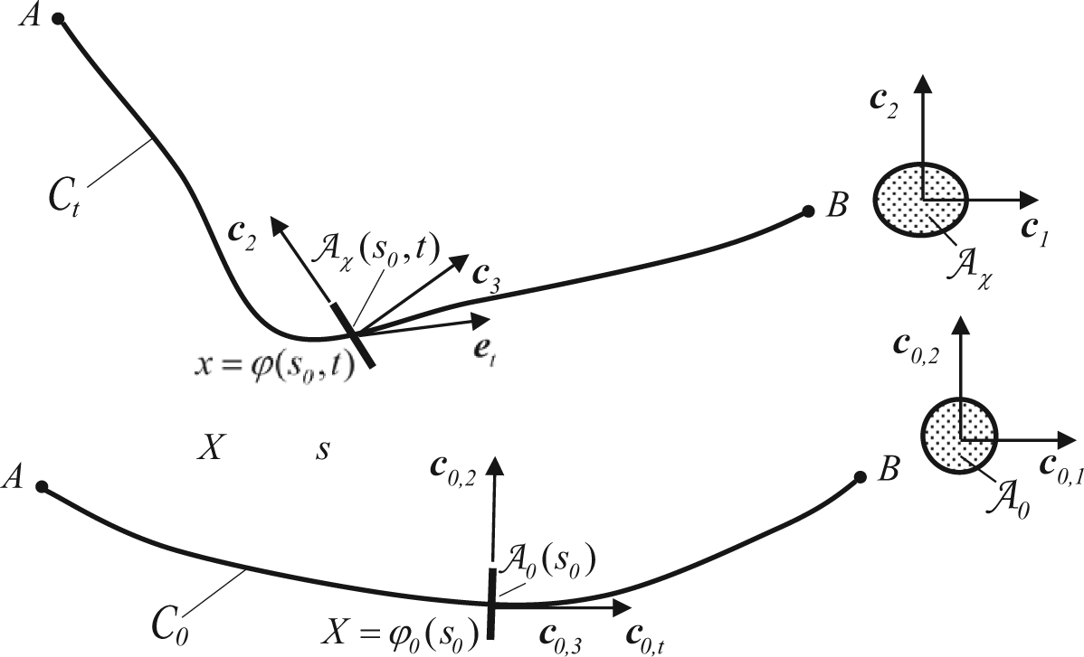
Consider a slender body $ℬ$ with a reference placement $ℬ_{0}$ in $ℰ$ . We assume that $ℬ_{0}$ is equipped with a base line (central line) $C_{0} \subseteq ℬ_{0}$ which is a parameterized, differentiable, bi-regular, open and simple curve in $ℰ$ , see appendix A.2 for the definitions. The material points at the endpoints of the beam base line are denoted A and B, respectively. The locations of these, in the reference placement, are given by X_A and X_B, respectively. Let $p \in ℬ$ denote an arbitrary material point on the base line with X as its place in the reference. Then X = φ₀(s₀) for some s₀ ∈ [0, L₀] where L₀ is the total arc-length of C₀ and $ϕ_{0} : [0, L_{0}] \in ℝ \to ℰ$ is the parameterization of C₀ using the arc-length as parameter, i.e. $C_{0} = {X \in ℰ | X = ϕ_{0} (s_{0}), s_{0} \in [0, L_{0}]}$ with φ₀(0) = X_A, φ₀(L₀) = X_B. Let the set of vectors e ₀(s₀) = ( e _0,n(s₀) e _0,b(s₀) e _0,t(s₀)) denote the Frenet frame of C₀ according to appendix A.1. The Darboux vector, corresponding to e ₀, is given by

δ_{0} (s_{0}) = e_{0, b} (s_{0}) κ_{0} (s_{0}) + e_{0, t} (s_{0}) τ_{0} (s_{0})

(1)

We introduce a second orthonormal frame associated with the central line. It is denoted by c ₀(s₀) = ( c _0,1(s₀) c _0,2(s₀) c _0,3(s₀)) where c _0,i(s₀) · c _0,j(s₀) = δ_ij. We take c _0,3(s₀) = e _0,t(s₀) and assume that c _0,i = c _0,i(s₀),i = 1, 2, 3 are continuously differentiable functions, then c ₀(s₀) = R ₀(s₀) e ₀(s₀) with $R_{0} (s_{0}) \in S O (V)$ and we may write

{\underline{c}}_{0} (s_{0}) = R_{0} (s_{0}) {\underline{e}}_{0} (s_{0}) = {\underline{e}}_{0} (s_{0}) (\begin{matrix} cos θ_{0} (s_{0}) & - sin θ_{0} (s_{0}) & 0 \\ sin θ_{0} (s_{0}) & cos θ_{0} (s_{0}) & 0 \\ 0 & 0 & 1 \end{matrix})

(2)

where θ₀ = θ₀(s₀) is continuously differentiable. This function may be arbitrarily chosen and gives some flexibility in the coordinate representation of the place X of a material point.

Remark 3.1: It is here assumed that the base line is bi-regular, see appendix A.1. If, for instance, κ₀(s₀) = 0, s₀ ∈ [0, L₀], then the base line is straight and the frame c ₀(s₀) may be chosen to contain constant vectors, i.e. vectors independent of s₀. In this case e ₀(s₀) and θ₀(s₀) are not uniquely defined. The choice of base line for the beam may be of some importance for the simplicity of the beam equations. This is, for instance, of significance when considering contact problems as discussed in Antman and Schuricht [17].

Lemma 3.1. We have

\frac{d {\underline{c}}_{0} (s_{0})}{d s_{0}} = ϑ_{0} (s_{0}) \times {\underline{c}}_{0} (s_{0})

(3)

where ϑ ₀(s₀) = e _0,b(s₀) κ ₀(s₀) + e _0,t(s₀)τ_0,c(s₀) is the Darboux vector corresponding to c ₀ and

τ_{0, c} (s_{0}) = τ_{0} (s_{0}) + \frac{d θ_{0} (s_{0})}{d s_{0}}

(4)

is the torsion of the frame c ₀.

Proof: The Darboux vector for c ₀ is the sum of the Darboux vector δ ₀ and the ‘angular velocity’ $e_{0, t} (s_{0}) \frac{d θ_{0} (s_{0})}{d s_{0}}$ of c ₀ relative to e ₀. This conclusion is obtained considering, for k = 1,

\begin{matrix} \frac{d c_{0, k}}{d s_{0}} = \frac{d e_{0, n}}{d s_{0}} cos θ_{0} + e_{0, n} (- sin θ_{0}) \frac{d θ_{0}}{d s_{0}} + \frac{d e_{0, b}}{d s_{0}} sin θ_{0} + e_{0, b} cos θ_{0} \frac{d θ_{0}}{d s_{0}} = δ_{0} \times e_{0, n} cos θ_{0} + \\ δ_{0} \times e_{0, b} sin θ_{0} + (e_{0, n} (- sin θ_{0}) + e_{0, b} cos θ) \frac{d θ_{0}}{d s_{0}} = δ_{0} \times c_{0, k} + c_{0, 2} \frac{d θ_{0}}{d s_{0}} = (δ_{0} + c_{0, 3} \frac{d θ_{0}}{d s_{0}}) \times c_{0, k} \\ = ϑ_{0} \times c_{0, k} \end{matrix}

where we have used the Frenet formulas (A.1.1). The demonstration for k = 2, 3 runs along similar lines.

Remark 3.2: The function θ₀ = θ₀(s₀) may be arbitrarily chosen. The coordinate system is called natural if θ₀(s₀) = 0,s₀ ∈ [0, L₀] and c ₀(s₀) = e ₀(s₀). Obviously, if one takes θ₀ = θ₀(s₀) to satisfy the differential equation

\frac{d θ_{0} (s_{0})}{d s_{0}} + τ_{0} (s_{0}) = 0, s_{0} \in [0, L_{0}]

(5)

i.e. $θ_{0} (s_{0}) = - \int_{0}^{s_{0}} τ_{0} (u) d u$ , then τ_0,c(s₀) = 0 and the Darboux vector is reduced to ϑ ₀(s₀) = e _0,b(s₀)κ₀(s₀). This coordinate system is called torsion free. We will encounter other possibilities further on.

The vectors c _0,1(s₀), c _0,2(s₀) span ‘the cross-sectional plane’ $P_{0} (s_{0})$ of the beam, placed at X = φ₀(s₀) in its reference placement. Put r (s₀, X₁, X₂) = c _0,1(s₀)X₁ + c _0,2(s₀)X₂, $(X_{1}, X_{2}) \in ℝ^{2}$ , then $P_{0} (s_{0}) = {X \in ℰ | X = \hat{X} (s_{0}, X_{1}, X_{2}) = ϕ_{0} (s_{0}) + r (s_{0}, X_{1}, X_{2}), (X_{1}, X_{2}) \in ℝ^{2}}$ . The ‘referential cross-section’ of the beam, $A_{0} (s_{0})$ is defined by $A_{0} (s_{0}) = P_{0} (s_{0}) \cap ℬ_{0}$ and the boundary curve of this cross-section is given by $\partial A_{0} (s_{0}) = P_{0} (s_{0}) \cap \partial ℬ_{0}$ . It is assumed that $A_{0} (s_{0}) \subseteq O_{0} (s_{0}, r)$ where $O_{0} (s_{0}, r_{0})$ is the open disc with radius r₀ > 0 and with its center located at X = φ₀(s₀), i.e.

O_{0} (s_{0}, r) = {X \in ℰ | X = \hat{X} (s_{0}, X_{1}, X_{2}) = ϕ_{0} (s_{0}) + r (s_{0}, X_{1}, X_{2}), X_{1}^{2} + X_{2}^{2} < r_{0}^{2}}

If the beam is slender enough we may take r₀ > 0 small enough so that (X₁, X₂, s₀) may be used as global coordinates in a tubular neighborhood $T N (r_{0})$ of the beam; see Proposition A.1.1 where a sufficient condition on r₀ for this to be the case, is demonstrated. In this paper a slender beam is defined by the requirement that for some 0 < ε < 1

r_{0} = ε \cdot min (r_{0, d}, κ_{0, m a x}^{- 1})

(6)

where r_0,d is defined in Lemma A.1.1 and $κ_{0, max} = sup_{s_{0} \in [0, L]} κ_{0} (s_{0})$ . Consider, for fixed s₀ ∈ [0, L₀], the bijective mapping $\overset{⌣}{X} (s_{0}) : O_{0} (s_{0}, r) \to D (r_{0}) = {(X_{1}, X_{2}) \in ℝ^{2} | X_{1}^{2} + X_{2}^{2} < r_{0}^{2}}$ defined by $\overset{⌣}{X} (s_{0}) (X) = (X_{1}, X_{2}) \Leftrightarrow X = \hat{X} (s_{0}, X_{1}, X_{2})$ with $\overset{⌢}{X} (s_{0}) = \overset{⌣}{X} {(s_{0})}^{- 1}$ then $\overset{⌢}{X} (s_{0}) (X_{1}, X_{2}) = \hat{X} (s_{0}, X_{1}, X_{2})$ . By introducing the set $Δ (s_{0}) = \overset{⌣}{X} (s_{0}) (A_{0} (s_{0})) \subseteq ℝ^{2}$ the reference placement of the beam may be written

ℬ_{0} = {X \in ℰ | X = \hat{X} (s_{0}, X_{1}, X_{2}) = ϕ_{0} (s_{0}) + r (s_{0}, X_{1}, X_{2}), s_{0} \in [0, L_{0}], (X_{1}, X_{2}) \in Δ (s_{0})}

The area of the cross-section $A_{0} (s_{0})$ is given by

a_{0} (s_{0}) = \int_{A_{0} (s_{0})} d a (X) = \int_{Δ (s_{0})} | \frac{\partial \overset{⌢}{X} (s_{0})}{\partial X_{1}} \times \frac{\partial \overset{⌢}{X} (s_{0})}{\partial X_{2}} | d X_{1} d X_{2} = \int_{Δ (s_{0})} | c_{0, 1} \times c_{0, 2} | d X_{1} d X_{2} = \int_{Δ (s_{0})} d X_{1} d X_{2}

Remark 3.3: If the base line is straight then, since κ₀(s₀) = 0, s₀ ∈ [0, L₀], one may use (s₀,X₁,X₂) as the global coordinates in the tubular neighborhood $T N (r_{0})$ for any r₀ > 0, cf. appendix A.1 and Simo [5].

Remark 3.4: One possible choice of c ₀ would be to take c ₀ equal to the principal basis corresponding to the area inertia tensor $A (s_{0}) \in S y m (V)$ , defined by

A (s_{0}) a = \int_{A_{0} (s_{0})} (X - ϕ_{0} (s_{0})) \times (a \times (X - ϕ_{0} (s_{0}))) d a (X), a \in V

Then A (s₀) c _0,i(s₀) = c _0,i(s₀)A_i(s₀), i = 1,2,3 where A_i(s₀), i = 1,2,3 are the principal area moments of inertia.

Let $χ : ℬ_{0} \times [0, T [\to ℬ_{t} \subseteq ℰ$ denote the transplacement of the beam from the reference placement $ℬ_{0}$ to the present placement $ℬ_{t}$ . We write x = χ(X, t). The base line of the beam, in its present placement, is given by

C_{t} = {x \in ℰ | x = ϕ (s_{0}, t), s_{0} \in [0, L_{0}]}

(7)

where φ(s₀, t) = χ(φ₀(s₀),t), s₀ ∈ [0, L₀]. The arc-length $s = \hat{s} (s_{0}, t), s_{0} \in [0, L_{0}]$ of the base line in its present placement is defined by $\hat{s} (s_{0}, t) = \int_{0}^{s_{0}} | \partial_{u} ϕ (u, t) | d u$ . Then $L (t) = \hat{s} (L_{0}, t)$ is the length of the base line in its present placement. Now since $\partial_{s_{0}} \hat{s} (s_{0}, t) = | \partial_{s_{0}} ϕ (s_{0}, t) | > 0$ the mapping $\hat{s} (\cdot, t) : [0, L_{0}] \to [0, L (t)]$ is invertible and we may write $s_{0} = {\hat{s}}^{- 1} (s, t), 0 \leq s \leq L (t)$ and then one has the parameterization $x = \hat{ϕ} (s, t) = ϕ ({\hat{s}}^{- 1} (s, t), t)$ 0 ≤ s ≤ L(t) of the base line and

e_{t} (s, t) = \frac{\partial \hat{ϕ} (s, t)}{\partial s} = \frac{\partial ϕ (s_{0}, t)}{\partial s_{0}} \frac{\partial {\hat{s}}^{- 1} (s, t)}{\partial s} = \frac{\partial ϕ (s_{0}, t)}{\partial s_{0}} {(\frac{\partial \hat{s} (s_{0}, t)}{\partial s_{0}})}^{- 1}

(8)

where e _t(s, t) is a unit tangent vector to C_t at $x = \hat{ϕ} (s, t)$ . We introduce the vector

γ (s_{0}, t) = \frac{\partial ϕ (s_{0}, t)}{\partial s_{0}} = F (ϕ_{0} (s_{0}), t) \frac{\partial ϕ_{0} (s_{0})}{\partial s_{0}} = F (ϕ_{0} (s_{0}), t) e_{0, t} (s_{0})

(9)

where F = ∂_Xχ is the deformation gradient. The length ratio associated with the transplacement of the base line is defined by l = l(s₀,t) = | F (φ₀(s₀),t) e _0,t(s₀)| and then, according to equation (8),

l = l (s_{0}, t) = | \frac{\partial \hat{s} (s_{0}, t)}{\partial s_{0}} | and γ (s_{0}, t) = e_{t} (\hat{s} (s_{0}, t), t) l (s_{0}, t)

(10)

What singles out the beam from other solid bodies is its elongated shape in all its placements. This property is manifested mathematically by the existence of a base line. The material points of the beam are assumed to be close to this base line in all of its placements. This is an assumption common to most beam theories. What distinguishes one beam theory from another is the set of constraints imposed on the possible transplacements of the beam. The set of transplacements considered in this paper is given by bijective mappings $χ : ℬ_{0} \times [0, T [\to ℬ_{t}$ of the form

x = χ (X, t) = χ (\hat{X} (s_{0}, X_{1}, X_{2}), t) = \hat{χ} (s_{0}, X_{1}, X_{2}, t) = φ (s_{0}, t) + p (s_{0}, X_{1}, X_{2}, t)

(11)

where $φ : [0, L_{0}] \times [0, T [\to ℰ$ is continuously differentiable and

p (s_{0}, X_{1}, X_{2}, t) = K (s_{0}, t) r (s_{0}, X_{1}, X_{2}) + u (s_{0}, X_{1}, X_{2}, t)

(12)

where $K : [0, L_{0}] \times [0, T [\to S O (V)$ is a continuously differentiable field on C₀ representing the rotation of the cross-section and

u (s_{0}, X_{1}, X_{2}, t) = c_{1} (s_{0}, t) u_{1} (s_{0}, X_{1}, X_{2}, t) + c_{2} (s_{0}, t) u_{2} (s_{0}, X_{1}, X_{2}, t) + c_{3} (s_{0}, t) u_{3} (s_{0}, X_{1}, X_{2}, t)

(13)

is the cross-sectional displacement field where the basis c (s₀, t) = ( c ₁(s₀, t), c ₂(s₀, t), c ₃(s₀, t)) is defined by

\underline{c} (s_{0}, t) = K (s_{0}, t) {\underline{c}}_{0} (s_{0})

(14)

The mappings $u_{i} : [0, L_{0}] \times Δ (s_{0}) \times [0, T [\to ℝ, i = 1, 2, 3$ are assumed to be differentiable. The position vector p may then be written

\begin{array}{l} p (s_{0}, X_{1}, X_{2}, t) = c_{1} (s_{0}, t) (X_{1} + u_{1} (s_{0}, X_{1}, X_{2}, t)) + \\ c_{2} (s_{0}, t) (X_{2} + u_{2} (s_{0}, X_{1}, X_{2}, t)) + c_{3} (s_{0}, t) u_{3} (s_{0}, X_{1}, X_{2}, t) \end{array}

(15)

If $u_{3} (s_{0}, X_{1}, X_{2}, t) = 0, \forall (s_{0}, X_{1}, X_{2}, t) \in [0, L_{0}] \times Δ (s_{0}) \times [0, T [$ then the cross-sectional displacement field is said to be in-plane. If u_i(s₀, X₁, X₂, t) = 0, i = 1, 2 then the displacement field is called out-of-plane. This represents a warping deformation of the cross-section.

Remark 3.5: In Antman [16] equations of constrained motion of beams are discussed at length. One class of transplacements considered there is given by (cf. equation (4.3(a)) in Antman [16])

p (s_{0}, X_{1}, X_{2}, t) = d_{1} (s_{0}, t) ϕ_{1} (s_{0}, X_{1}, X_{2}, t) + d_{2} (s_{0}, t) ϕ_{2} (s_{0}, X_{1}, X_{2}, t) + d_{3} (s_{0}, t) ϕ_{3} (s_{0}, X_{1}, X_{2}, t)

(16)

where d _i = d _i(s₀, t), i = 1, 2, 3 are (general) director fields. Obviously equation (15) may be considered as a special case of equation (16) with the constraint conditions d _i· d _j = δ_ij, i,j = 1, 2, 3.

The transplacements defined in equation (11) are ‘parameterized’ by the mappings

φ : [0, L_{0}] \times [0, T [\to ℰ, K : [0, L_{0}] \times [0, T [\to S O (V), u_{i} : T N (r_{0}) \times [0, T [\to ℝ, i = 1, 2

The transplacements will include bending, torsion, shear and warping of the beam. The incorporation of general cross-sectional displacement fields is a new feature in this beam theory as compared to the one presented in Simo [5] and Simo and Vu-Quoc [10].

The base line of the beam, in its present placement, is given by

C_{t} = {x \in ℰ | x = \hat{χ} (s_{0}, 0, 0, t) = φ (s_{0}, t) + p (s_{0}, 0, 0, t), s_{0} \in [0, L_{0}]}

(17)

where, according to equation (11), p (s₀, 0, 0, t) = K (s₀, t) r (s₀, 0, 0) + u (s₀, 0, 0, t) = u (s₀, 0, 0, t). By comparing equations (7) and (17) one obtains the relation φ(s₀, t) = ϕ(s₀, t) + u (s₀, 0, 0, t), s₀ ∈ [0, L₀] and the transplacement may now be written

x = \hat{χ} (s_{0}, X_{1}, X_{2}, t) = ϕ (s_{0}, t) + p (s_{0}, X_{1}, X_{2}, t) - u (s_{0}, 0, 0, t)

(18)

Obviously, if u (s₀, 0, 0, t) = 0, s₀ ∈ [0, L₀] then the transplacement is given by

x = \hat{χ} (s_{0}, X_{1}, X_{2}, t) = ϕ (s_{0}, t) + p (s_{0}, X_{1}, X_{2}, t)

(19)

and the base line, in its present placement, by

C_{t} = {x \in ℰ | x = \hat{χ} (s_{0}, 0, 0, t) = ϕ (s_{0}, t), s_{0} \in [0, L_{0}]}

The cross-section $A_{χ}$ of the beam in its present placement, is given by the set

A_{χ} (s_{0}, t) = {x \in ℰ | x = \hat{x} (s_{0}, X_{1}, X_{2}) = ϕ (s_{0}, t) + p (s_{0}, X_{1}, X_{2}, t), (X_{1}, X_{2}) \in Δ (s_{0})}

The area of this cross-section is

a (s_{0}, t) = \int_{A_{χ} (s_{0}, t)} d a (x) = \int_{Δ (s_{0})} A (s_{0}, X_{1}, X_{2}, t) d X_{1} d X_{2}

where A is the area ratio defined by $A = | \frac{\partial p}{\partial X_{1}} \times \frac{\partial p}{\partial X_{2}} | = \sqrt{A_{1}^{2} + A_{2}^{2} + A_{3}^{2}}$ where

\begin{array}{l} A_{1} & = & \frac{\partial u_{2}}{\partial X_{1}} \frac{\partial u_{3}}{\partial X_{2}} - \frac{\partial u_{3}}{\partial X_{1}} \frac{\partial u_{2}}{\partial X_{2}} - \frac{\partial u_{3}}{\partial X_{1}}, A_{2} = \frac{\partial u_{3}}{\partial X_{1}} \frac{\partial u_{1}}{\partial X_{2}} - \frac{\partial u_{3}}{\partial X_{2}} \frac{\partial u_{1}}{\partial X_{1}} - \frac{\partial u_{3}}{\partial X_{2}} \\ A_{3} & = & 1 + \frac{\partial u_{1}}{\partial X_{1}} + \frac{\partial u_{2}}{\partial X_{2}} + \frac{\partial u_{1}}{\partial X_{1}} \frac{\partial u_{2}}{\partial X_{2}} - \frac{\partial u_{2}}{\partial X_{1}} \frac{\partial u_{1}}{\partial X_{2}} \end{array}

The vector

A = c_{1} A_{1} + c_{2} A_{2} + c_{3} A_{3}

(20)

is called the area ratio vector. Considering an in-plane displacement one obtains A₁ = A₂ = 0 and then

A = | A_{3} | = | 1 + \frac{\partial u_{1}}{\partial X_{1}} + \frac{\partial u_{2}}{\partial X_{2}} + \frac{\partial u_{1}}{\partial X_{1}} \frac{\partial u_{2}}{\partial X_{2}} - \frac{\partial u_{1}}{\partial X_{2}} \frac{\partial u_{2}}{\partial X_{1}} |

for the area ratio. The transplacement is then said to be (cross-section) area preserving if A = 1, i.e. if ∂_X₁u₁ + ∂_X₂u₂ + ∂_X₁u₁∂_X₂u₂ − ∂_X₂u₁∂_X₁u₂ = 0.

Remark 3.6: By taking u_i(s₀, X₁, X₂, t) = 0, i = 1, 2, 3 the transplacement in equation (11) results in ‘rigid cross-sections’ which precludes changes of shape of the cross-sections. By taking u_i(s₀, X₁, X₂, t) = q_i(s₀, t)X_i, i = 1, 2, and u₃(s₀, X₁, X₂, t) = 0 where q_i: [0, L₀] × [0, T[→]−1, ∞[ is a differentiable mapping, the displacement u will represent a simple in-planecontraction/expansion of the cross-section along the c ₁ - and c ₂-axes, respectively. The area ratio of this mapping is given by A(s₀, t) = |(1 + q₁(s₀, t))(1 + q₂(s₀, t))|.

Remark 3.7: By taking u₃(s₀, X₁, X₂, t) = f(s₀, X₁, X₂)q(s₀, t) and u_i(s₀, X₁, X₂, t) = 0, i = 1,2, where $f : [0, L_{0}] \times Δ (s_{0}) \times [0, T [\to ℝ$ and $q : [0, L_{0}] \times [0, T [\to ℝ$ are differentiable mappings, the displacement u will represent a simple out-of-plane displacement along the c ₃-axis. In this case $A_{1} = - q \partial_{X_{1}} f$ and $A_{2} = - q \partial_{X_{2}} f$ and $A = \sqrt{1 + q^{2} ({(\partial_{X_{1}} f)}^{2} + {(\partial_{X_{2}} f)}^{2})}$ .

Remark 3.8: The set of vectors e (s) = ( e _n(s) e _b(s) e _t(s)) denote the Frenet frame of base line C_t in its present placement. We may write c (s, t) = R (s, t) e (s, t), where $R (s, t) \in S O (V)$ . The relation between the Frenet frames of the base line in the referential and present placements is then given by

\underline{e} = R^{T} K R_{0} {\underline{e}}_{0}

(21)

The cross-section plane of the beam in its present placement

P (s, t) = {x \in ℰ | x = \hat{ϕ} (s, t) + e_{n} (s, t) x_{1} + e_{b} (s, t) x_{2}, (x_{1}, x_{2}) \in ℝ^{2}}

and the spatial cross-sections of the beam are then given by $A (s, t) = ℬ_{t} \cap P (s, t)$ . If we assume that the beam, in its present placement, is slender enough and that its curvature κ = κ(s, t) is small enough then (s, x₁, x₂) may be used as tubular coordinates for the beam in its present placement. See Proposition A.1.1. This will however, due to the deformation of the beam, not always be possible.

Next we derive some useful kinematical relations.

Lemma 3.2. We have

\frac{\partial K (s_{0}, t)}{\partial s_{0}} = λ (s_{0}, t) \times K (s_{0}, t) and \frac{\partial K (s_{0}, t)}{\partial t} = ω (s_{0}, t) \times K (s_{0}, t)

(22)

where

λ (s_{0}, t) = a x (\frac{\partial K (s_{0}, t)}{\partial s_{0}} K {(s_{0}, t)}^{T}) and ω (s_{0}, t) = a x (\frac{\partial K (s_{0}, t)}{\partial t} K {(s_{0}, t)}^{T})

(23)

Proof: This follows by differentiating the relation $K (s_{0}, t) K {(s_{0}, t)}^{T} = 1_{V}$ with respect to s₀ and t, respectively.

Proposition 3.1. We have

\frac{\partial \underline{c} (s_{0}, t)}{\partial s_{0}} = ψ (s_{0}, t) \times \underline{c} (s_{0}, t) and \frac{\partial \underline{c} (s_{0}, t)}{\partial t} = ω (s_{0}, t) \times \underline{c} (s_{0}, t)

(24)

where

ψ (s_{0}, t) = λ (s_{0}, t) + ϑ (s_{0}, t), ϑ (s_{0}, t) = K (s_{0}, t) ϑ_{0} (s_{0})

(25)

is the Darboux vector corresponding to c in the referential description and ω (s₀,t) is the angular velocity vector of c . Furthermore

\dot{p} = \frac{\partial p}{\partial t} = ω \times p + {\dot{u}}^{r e l}, \frac{\partial p}{\partial s_{0}} = ψ \times p + α

(26)

where ${\dot{u}}^{r e l} = c_{1} {\dot{u}}_{1} + c_{2} {\dot{u}}_{2} + c_{3} {\dot{u}}_{3}$ , ${\dot{u}}_{i} = \partial_{t} u_{i}, i = 1, 2, 3$ and $α = c_{1} \partial_{s_{0}} u_{1} + c_{2} \partial_{s_{0}} u_{2} + c_{3} \partial_{s_{0}} u_{3}$ .

Proof: By differentiating equation (14) and using Lemmas 3.1 and 3.2 one obtains

\begin{matrix} \frac{\partial \underline{c}}{\partial s_{0}} = \frac{\partial K}{\partial s_{0}} {\underline{c}}_{0} + K \frac{d {\underline{c}}_{0}}{\partial s_{0}} = λ \times K {\underline{c}}_{0} + K (ϑ_{0} \times {\underline{c}}_{0}) = (λ + ϑ) \times \underline{c} = ψ \times c_{i} \\ \frac{\partial \underline{c}}{\partial t} = \frac{\partial K}{\partial t} {\underline{c}}_{0} = ω \times K {\underline{c}}_{0} = ω \times \underline{c} \end{matrix}

Furthermore, since p = c ₁(X₁ + u₁) + c ₂(X₂ + u₂) + c ₃u₃

\begin{matrix} \dot{p} = \frac{\partial c_{1}}{\partial t} (X_{1} + u_{1}) + c_{1} \frac{\partial u_{1}}{\partial t} + \frac{\partial c_{2}}{\partial t} (X_{2} + u_{2}) + c_{2} \frac{\partial u_{2}}{\partial t} + \frac{\partial c_{3}}{\partial t} u_{3} + c_{3} \frac{\partial u_{3}}{\partial t} = \\ ω \times c_{1} (X_{1} + u_{1}) + c_{1} \frac{\partial u_{1}}{\partial t} + ω \times c_{2} (X_{2} + u_{2}) + c_{2} \frac{\partial u_{2}}{\partial t} + ω \times c_{3} u_{3} + c_{3} \frac{\partial u_{3}}{\partial t} = ω \times p + {\dot{u}}^{r e l} \\ \frac{\partial p}{\partial s_{0}} = \frac{\partial c_{1}}{\partial s_{0}} (X_{1} + u_{1}) + c_{1} \frac{\partial u_{1}}{\partial s_{0}} + \frac{\partial c_{2}}{\partial s_{0}} (X_{2} + u_{2}) + c_{2} \frac{\partial u_{2}}{\partial s_{0}} + \frac{\partial c_{3}}{\partial s_{0}} u_{3} + c_{3} \frac{\partial u_{3}}{\partial s_{0}} = \\ ψ \times p + c_{1} \frac{\partial u_{1}}{\partial s_{0}} + c_{2} \frac{\partial u_{2}}{\partial s_{0}} + c_{3} \frac{\partial u_{2}}{\partial s_{0}} \end{matrix}

Remark 3.9:A rigid transplacement of the beam is given by

x = χ (X, t) = x_{A} (t) + Q (t) (X - X_{A}), X \in ℬ_{0}, t \in [0, T [

where $x_{A} (t) \in ℰ$ is the present place of the beam endpoint A and $Q (t) \in S O (V)$ is the rotation of the beam. Then $ϕ (s_{0}, t) = x_{A} + Q (t) (ϕ_{0} (s_{0}) - X_{A}), X \in ℬ_{0}, t \in [0, T [$ and consequently e (s, t) = Q (t) e ₀(s₀), κ(s, t) = κ₀(s₀) and τ(s, t) = τ₀(s₀). According to Lemma 3.2 the Darboux vector ψ , corresponding to the frame c , is the sum of a vector λ representing the change of the cross-sectional rotations along the beam and ϑ = Kϑ ₀, where K is the rotation of the cross-section and ϑ ₀ is the Darboux vector of c ₀. If e denotes the Frenet frame of C_t then, if c = Re

\frac{\partial \underline{c}}{\partial s} = \frac{\partial R}{\partial s} \underline{e} + R \frac{\partial \underline{e}}{\partial s} = \frac{\partial R}{\partial s} R^{T} \underline{c} + R (δ \times \underline{e}) = Ω \underline{c} + R (δ \times \underline{e}) = (Ω + R δ) \times \underline{c}

where δ = e _b κ + e _tτ is the Darboux vector of the frame e and $Ω = a x (\frac{\partial R}{\partial s} R^{T})$ . On the other hand, according to equation (24)₁, $\partial_{s} \underline{c} = \partial_{s_{0}} \underline{c} \partial_{s} {\hat{s}}^{- 1} = \frac{1}{l} ψ \times \underline{c}$ and consequently ψ = l(Ω + Rδ ) = l(Ω + R ( e _bκ + e _tτ)). From equation (25) one obtains the relation ψ = λ + K ( e _0,b κ ₀ + e _0,tτ_0,c) and then

λ = ψ - K (e_{0, b} κ_{0} + e_{0, t} τ_{0, c}) = l (Ω + R (e_{b} κ + e_{t} τ)) - K (e_{0, b} κ_{0} + e_{0, t} τ_{0, c}))

But according to equation (21)

R (e_{b} κ + e_{t} τ_{c}) = R R^{T} K R_{0} (e_{0, b} κ + e_{0, t} τ_{c}) = K R_{0} (e_{0, b} κ + e_{0, t} τ_{c})

and then

λ = l Ω + K ((l κ R_{0} - κ_{0} 1_{V}) e_{0, b} + (l τ R_{0} - τ_{0, c} 1_{V}) e_{0, t}))

Using natural coordinates $R_{0} = 1_{V}$ and τ_0,c = τ₀ then

λ = l Ω + K ((l κ - κ_{0}) e_{0, b} + (l τ - τ_{0}) e_{0, t}))

Considering a transplacement with l = 1, κ = κ₀ and τ = τ₀ one obtains λ = Ω. According to the fundamental theorem of curves (cf. Choquet-Bruhat et al. [18]) there exists, in this case, a $Q = Q (t) \in S O (V)$ such that e = Qe ₀. Thus, by comparing with equation (21), we have R ^T K = Q and then K = RQ . A rigid transplacement of the beam is now characterized by K = Q and then $R = 1_{V}$ , Ω = 0 and λ = 0.

The relationship between λ and ω is expressed in the following compatibility conditions (cf. Antman [16, equation (2.9(b))]).

Proposition 3.2. We have

\dot{λ} = \frac{\partial ω}{\partial s_{0}} + ω \times λ, \dot{ψ} = \frac{\partial ω}{\partial s_{0}} + ω \times ψ

(27)

Proof: By direct computation

\dot{λ} = \frac{\partial λ}{\partial t} = a x (\frac{\partial^{2} K}{\partial t \partial s_{0}} K^{T} + \frac{\partial K}{\partial s_{0}} \frac{\partial K}{\partial t^{T}}), \frac{\partial ω}{\partial s_{0}} = a x (\frac{\partial^{2} K}{\partial s_{0} \partial t} K^{T} + \frac{\partial K}{\partial t} {\frac{\partial K}{\partial s_{0}}}^{T})

Thus, if $\frac{\partial^{2} K}{\partial t \partial s_{0}} = \frac{\partial^{2} K}{\partial s_{0} \partial t}$ then

\dot{λ} = \frac{\partial ω}{\partial s_{0}} - a x (\frac{\partial K}{\partial t} {\frac{\partial K}{\partial s_{0}}}^{T} - \frac{\partial K}{\partial s_{0}} \frac{\partial K}{\partial t^{T}}) = \frac{\partial ω}{\partial s_{0}} - a x ((ω \times 1) K {\frac{\partial K}{\partial s_{0}}}^{T} - \frac{\partial K}{\partial s_{0}} K^{T} {(ω \times 1)}^{T}) = \frac{\partial ω}{\partial s_{0}} + ω \times λ

Furthermore, since $\dot{ϑ} = \dot{K} ϑ_{0} = ω \times K ϑ_{0} = ω \times ϑ$ one has

\dot{ψ} = \dot{λ} + \dot{ϑ} = \frac{\partial ω}{\partial s_{0}} + ω \times λ + ω \times ϑ = \frac{\partial ω}{\partial s_{0}} + ω \times (λ + ϑ) = \frac{\partial ω}{\partial s_{0}} + ω \times ψ

The kinematics of the beam is given by the mapping in equation (19). From φ, representing the present placement of the central line and K representing the rotation of the cross-sections, the deformation measures λ and ψ have been defined according to equations (23) and (25), respectively. The in-cross-sectional displacement is represented by the mappings u_i, i = 1, 2, 3. The associated deformation measures are given by $α = c_{1} \partial_{s_{0}} u_{1} + c_{2} \partial_{s_{0}} u_{2} + c_{3} \partial_{s_{0}} u_{3}$ and $\nabla_{X} u = \partial_{X_{1}} u \otimes h_{0}^{1} + \partial_{X_{2}} u \otimes h_{0}^{2}$ . We have

\frac{\partial u}{\partial s_{0}} = ψ \times u + α, \frac{\partial p}{\partial s_{0}} = ψ \times K r + \frac{\partial u}{\partial s_{0}}

(28)

and the gradient of the in-cross-sectional displacement is then given by (cf. (A.2.7))

\nabla u = \nabla_{X} u + (ψ \times u + α) \otimes h_{0}^{3}

Furthermore

\dot{u} = \frac{\partial u}{\partial t} = ω \times u + {\dot{u}}^{r e l}, \frac{\partial \dot{u}}{\partial s_{0}} = \dot{ψ} \times u + ψ \times \dot{u} + \dot{α}

The material velocity and acceleration are defined by $\dot{x} = \partial_{t} χ$ , $\ddot{x} = \partial_{t}^{2} χ$ .

Proposition 3.3. We have

\begin{array}{l} \dot{x} & = & {\dot{x}}_{c} + ω \times p + {\dot{u}}^{rel} \\ \ddot{x} & = & {\ddot{x}}_{c} + \dot{ω} \times p + ω \times (ω \times p) + 2 ω \times {\dot{u}}^{rel} + {\ddot{u}}^{rel} \end{array}

(29)

where ${\dot{x}}_{c} (s_{0}, t) = \partial_{t} ϕ (s_{0}, t)$ is the velocity and ${\ddot{x}}_{c} (s_{0}, t) = \partial_{t}^{2} ϕ (s_{0}, t)$ the acceleration of the cross-sectional center, and ${\ddot{u}}^{rel} = c_{1} {\ddot{u}}_{1} + c_{2} {\ddot{u}}_{2} + c_{3} {\ddot{u}}_{3}$ , ${\ddot{u}}_{i} = \partial_{t}^{2} u_{i}, i = 1, 2, 3$ . Note that $\partial_{s_{0}} {\dot{x}}_{c} = \dot{γ}$ .

Proof: According to equation (19) x = φ + p where p = c ₁(X₁ + u₁) + c ₂(X₂ + u₂) + c ₃u₃. Then, using equation (26)₁, one obtains

\dot{x} = \partial_{t} \hat{χ} = \frac{\partial ϕ}{\partial t} + \dot{p} = \frac{\partial ϕ}{\partial t} + ω \times p + {\dot{u}}^{r e l}

Furthermore

\begin{array}{l} \ddot{x} & = & \partial_{t}^{2} \hat{χ} = {\ddot{x}}_{c} + \dot{ω} \times p + ω \times \dot{p} + {\dot{c}}_{1} \frac{\partial u_{1}}{\partial t} + c_{1} \frac{\partial^{2} u_{1}}{\partial t^{2}} + {\dot{c}}_{2} \frac{\partial u_{2}}{\partial t} + c_{2} \frac{\partial^{2} u_{2}}{\partial t^{2}} \\ = & {\ddot{x}}_{c} + \dot{ω} \times p + ω \times (ω \times (p + c_{1} {\dot{u}}_{1} + c_{2} {\dot{u}}_{2})) + ω \times (c_{1} {\dot{u}}_{1} + c_{2} {\dot{u}}_{2}) + c_{1} {\ddot{u}}_{1} + c_{2} {\ddot{u}}_{2} \\ = & {\ddot{x}}_{c} + \dot{ω} \times p + ω \times (ω \times p) + 2 ω \times {\dot{u}}^{rel} + {\ddot{u}}^{rel} \end{array}

and this proves the proposition.

We are now in the position to be able to express the deformation gradient F = ∂_Xχ in terms of the vectors γ and ψ . We refer to appendix A.2 for the definitions and formulas concerning the coordinate representation of the beam in its reference placement

X = \hat{X} (s_{0}, X_{1}, X_{2}) = ϕ_{0} (s_{0}) + r (s_{0}, X_{1}, X_{2}), s_{0} \in [0, L_{0}], (X_{1}, X_{2}) \in Δ (s_{0})

and the associated basis h ₀(s₀) = ( h _0,1(s₀) h _0,2(s₀) h _0,3(s₀)) and its reciprocal basis ${\bar{h}}_{0} (s_{0})$ .

Proposition 3.4. We have

F = π + \frac{1}{h_{0}} σ \otimes c_{0, 3}

(30)

where

σ = γ + ψ \times p + α and π = \nabla_{X} p = \sum_{i = 1}^{2} c_{i} \otimes h_{0}^{i} + \nabla_{X} u

(31)

and h₀ = 1 + e _0,t· δ ₀ × r , cf. Appendix A.2.

Proof: The deformation gradient is given by

F = \frac{\partial χ}{\partial X} = \frac{\partial \hat{χ}}{\partial X_{1}} \otimes h_{0}^{1} + \frac{\partial \hat{χ}}{\partial X_{2}} \otimes h_{0}^{2} + \frac{\partial \hat{χ}}{\partial s_{0}} \otimes h_{0}^{3}

and then from Proposition 3.1 it follows that

\frac{\partial \hat{χ}}{\partial s_{0}} = \frac{\partial ϕ}{\partial s_{0}} + \frac{\partial p}{\partial s_{0}} = \frac{\partial ϕ}{\partial s_{0}} + ψ \times K r + \frac{\partial u}{\partial s_{0}}

where we have used equation (28)₂. Furthermore

\frac{\partial \hat{χ}}{\partial X_{1}} = c_{1} (1 + \frac{\partial u_{1}}{\partial X_{1}}) + c_{2} \frac{\partial u_{2}}{\partial X_{1}} + c_{3} \frac{\partial u_{3}}{\partial X_{1}} and \frac{\partial \hat{χ}}{\partial X_{2}} = c_{1} \frac{\partial u_{1}}{\partial X_{2}} + c_{2} (1 + \frac{\partial u_{2}}{\partial X_{2}}) + c_{3} \frac{\partial u_{3}}{\partial X_{2}}

Consequently

\begin{array}{l} F & = & (c_{1} (1 + \frac{\partial u_{1}}{\partial X_{1}}) + c_{2} \frac{\partial u_{2}}{\partial X_{1}} + c_{3} \frac{\partial u_{3}}{\partial X_{1}}) \otimes h_{0}^{1} + (c_{1} \frac{\partial u_{1}}{\partial X_{2}} + c_{2} (1 + \frac{\partial u_{2}}{\partial X_{2}}) + c_{3} \frac{\partial u_{3}}{\partial X_{2}}) \otimes h_{0}^{2} \\ + (\frac{\partial ϕ}{\partial s_{0}} + ψ \times K r + \frac{\partial u}{\partial s_{0}}) \otimes h_{0}^{3} = \sum_{i = 1}^{2} c_{i} \otimes h_{0}^{i} + \nabla_{X} u + (γ + ψ \times p + α) \otimes h_{0}^{3} \\ = & π + σ \otimes h_{0}^{3} = π + \frac{1}{h_{0}} σ \otimes c_{0, 3} \end{array}

This concludes the proof.

Remark 3.10: Note that, according to equation (26)₂ and equation (31)₁ we have ∂_s₀ p = σ − γ .

Remark 3.11: According to the previous proof we have $F c_{0, 1} = c_{1} + \partial_{X_{1}} u$ , $F c_{0, 2} = c_{2} + \partial_{X_{2}} u$ , $F c_{0, 3} = π c_{0, 3} + \frac{1}{h_{0}} σ$ where $π c_{0, 3} = ((c_{1} + \partial_{X_{1}} u) X_{2} - (c_{2} + \partial_{X_{2}} u) X_{1}) \frac{τ_{0, c}}{h_{0}}$ . Thus the basis c is not equal to the convected basis. If the coordinate system is torsion free then πc _0,3 = 0 and $F c_{0, 3} = \frac{1}{h_{0}} σ$ . On the base line (X₁ = X₂ = 0) we have h₀ = 1, p = 0 , and then according to (26)₂, $α = {c_{1} \partial_{s_{0}} u_{1} + c_{2} \partial_{s_{0}} u_{2} + c_{3} \partial_{s_{0}} u_{3} |}_{X_{1} = X_{2} = 0} = 0$ , and consequently Fc _0,3 = γ in accordance with equation (7).

Remark 3.12: Using natural coordinates we have ϑ ₀ = δ ₀ = e _0,bκ₀ + e _0,tτ₀ and then

ψ = λ + K ϑ_{0} = λ + κ_{0} K e_{0, b} + τ_{0} K e_{0, t}

Using torsion free coordinates, i.e. if τ_0,c(s₀) = 0, s₀ ∈ [0, L₀], we have ϑ ₀ = e _0,bκ₀ and then

ψ = λ + K ϑ_{0} = λ + κ_{0} K e_{0, b}

In this case, according to equation (A.2.5), $h_{0}^{i} = c_{0, i}, i = 1, 2$ and then $π = K (1_{V} - c_{0, 3} \otimes c_{0, 3}) + \nabla_{X} u$ . Hence

\begin{array}{l} σ & = & γ + ψ \times p + α = γ + λ \times K r + \frac{\partial u}{\partial s_{0}} + ϑ \times K r = γ + λ \times K r + \frac{\partial u}{\partial s_{0}} + κ_{0} K (e_{0, b} \times r_{0}) \\ F & = & K (1_{V} - c_{0, 3} \otimes c_{0, 3}) + \nabla_{X} u + \frac{1}{h_{0}} (γ + λ \times K r + \frac{\partial u}{\partial s_{0}} + κ_{0} K (e_{0, b} \times r_{0})) \otimes c_{0, 3} \\ = & K (1_{V} - (c_{0, 3} - \frac{1}{h_{0}} κ_{0} (e_{0, b} \times r_{0})) \otimes c_{0, 3}) + \nabla_{X} u + \frac{1}{h_{0}} \frac{\partial u}{\partial s_{0}} \otimes c_{0, 3} + \frac{1}{h_{0}} (γ + λ \times K r) \otimes c_{0, 3} \end{array}

But e _0,b × r ₀ = α c _0,3 where $α = c_{0, 3} \cdot e_{0, b} \times r_{0} = e_{0, t} \times e_{0, b} \cdot r_{0} = - e_{0, n} \cdot r_{0} = - \frac{1}{κ_{0}} (1 - h_{0})$ since h₀ = 1 − e _0,n· r κ₀ and then

(c_{0, 3} - \frac{1}{h_{0}} κ_{0} (e_{0, b} \times r_{0})) \otimes c_{0, 3} = (c_{0, 3} + \frac{κ_{0}}{h_{0}} \frac{1}{κ_{0}} (1 - h_{0}) c_{0, 3}) \otimes c_{0, 3} = \frac{1}{h_{0}} c_{0, 3} \otimes c_{0, 3}

which gives

F = K (1_{V} - \frac{1}{h_{0}} c_{0, 3} \otimes c_{0, 3}) + \nabla u + \frac{1}{h_{0}} (γ + λ \times K r) \otimes c_{0, 3}

We summarize this in the following corollary.

Corollary 3.1. We have

F = K (1_{V} - \frac{1}{h_{0}} e_{0, t} \otimes e_{0, t}) + \nabla u + \frac{1}{h_{0}} (γ + λ \times K r) \otimes e_{0, t}

(32)

Remark 3.13: The deformation gradient F is, by its definition, independent of the coordinate system used. Note that the representation of the deformation gradient given in equation (32) does not depend on the frame c ₀.

The shearing vector s is defined by $s = c_{3} - e_{t} = c_{3} - γ \frac{1}{l}$ . The shear angle of the cross-section is the angle ς between the vectors c ₃ and e _t. i.e. cos ς = c ₃· e _t = 1 − c ₃· s . No shearing is characterized by s = 0. The assumed bijectivity of the transplacement $χ : ℬ_{0} \times [0, T [\to ℬ_{t}$ implies the condition

det F (X, t) > 0, X \in ℬ_{0}, t \in [0, T [

(33)

Proposition 3.5. The condition in equation (33) is equivalent to

A \cdot σ > 0, X \in ℬ_{0}, t \in [0, T [

(34)

where A is the area ratio vector defined in equation (20).

Proof: A direct computation gives the volume ratio

det F = F c_{0, 1} \times F c_{0, 2} \cdot F c_{0, 3} = π c_{0, 1} \times π c_{0, 2} \cdot σ \frac{1}{h_{0}}

(35)

where $π c_{0, 1} \times π c_{0, 2} = \partial_{X_{1}} p \times \partial_{X_{2}} p = A$ . Then $det F = A \cdot σ \frac{1}{h_{0}}$ and since h₀ > 0 the proposition follows.

Remark 3.14: In the case of an in-plane displacement field, one has A₁ = A₂ = 0. From equation (34), one then obtains $det F = \frac{A_{3}}{h_{0}} (c_{3} \cdot γ + c_{3} \cdot ψ \times p)$ and with A₃ > 0 the condition in equation (33) is equivalent to

l cos ς + c_{3} \times ψ \cdot p > 0, X \in ℬ_{0}, t \in [0, T [

(36)

In the absence of shear, i.e. if s = 0, we have ς = 0 and c ₃ = e _t and then from $\partial_{s_{0}} c_{3} = ψ \times c_{3}$ it follows that $ψ \times c_{3} = \partial_{s_{0}} c_{3} = \partial_{s_{0}} e_{t} = \partial_{s_{0}} \hat{s} \partial_{s} e_{t} = l κ e_{n}$ . Thus l cos ς + c ₃ × ψ · p = l − ψ × c ₃· p = l(1 − κ e _n· p ) = l(1 − κ p _n) where p _n = e _n· p . The condition in equation (36) is then reduced to κp_n < 1. Thus in the absence of shear, and if A₃ > 0, then det F (X, t) > 0 ⇔ κp_n < 1. For the simple in-plane contraction/expansion of the cross-section, as defined in Remark 3.6, this is fulfilled if, for instance

κ | p | \leq κ \sqrt{X_{1}^{2} + X_{2}^{2}} \sqrt{{(1 + q_{1})}^{2} + {(1 + q_{2})}^{2}} < κ r_{0} \sqrt{{(1 + q_{1})}^{2} + {(1 + q_{2})}^{2}} < 1

or, according to equation (6)

κ \sqrt{{(1 + q_{1})}^{2} + {(1 + q_{2})}^{2}} < \frac{1}{r_{0}} = \frac{1}{ε \cdot min (r_{0, d}, κ_{0, m a x}^{- 1})}

Remark 3.15: By using the representations

γ = c_{1} γ_{1} + c_{2} γ_{2} + c_{3} γ_{3}, ψ = c_{1} ψ_{1} + c_{2} ψ_{2} + c_{3} ψ_{3}, p = c_{1} (X_{1} + u_{1}) + c_{2} (X_{2} + u_{2}) + c_{3} u_{3}

one obtains the condition

\begin{array}{l} c_{3} \cdot γ + c_{3} \cdot ψ \times p = γ_{3} + c_{3} \cdot ψ \times p = γ_{3} + c_{3} \times (c_{1} ψ_{1} + c_{2} ψ_{2} + c_{3} ψ_{3}) \cdot p \\ = γ_{3} + (c_{2} ψ_{1} + c_{1} (- ψ_{2})) \cdot p = γ_{3} + ψ_{1} (X_{2} + u_{2}) + (- ψ_{2}) (X_{1} + u_{1}) > 0 \end{array}

γ_{3} (s_{0}, t) > ψ_{2} (s_{0}, t) (X_{1} + u_{1} (s_{0}, X_{1}, X_{2}, t)) - ψ_{1} (s_{0}, t) (X_{2} + u_{2} (s_{0}, X_{1}, X_{2}, t))

for all $(s_{0}, X_{1}, X_{2}) \in T N (r_{0})$ . This is equivalent to conditions (7.8) and (7.9) on p. 285 in Antman [16]. A general characterization of the condition $det F (X, t) > 0, X \in ℬ_{0}, t \in [0, T [$ for special Cosserat rods is presented in Antman [16, Theorem 7.2, pp. 284–287].

Remark 3.16: In the case of a simple out-of-plane displacement, we have $A_{1} = - q \partial_{X_{1}} f$ , $A_{2} = - q \partial_{X_{2}} f$ and A₃ = 0. Then $det F = - q (c_{1} \partial_{X_{1}} f + c_{2} \partial_{X_{2}} f) \cdot (γ + ψ \times p)$ where p = c ₁X₁ + c ₂X₂ + c ₃fq. The condition in equation (33) may then be written

q (γ_{1} + ψ_{2} f q - ψ_{3} X_{2}) \partial_{X_{1}} f + (γ_{2} + ψ_{1} f q + ψ_{3} X_{1}) \partial_{X_{2}} f) < 0

Apart from the deformation gradient F itself we will need an expression for its time derivative $\dot{F}$ given in terms of the introduced deformation measures γ , ψ , α and π . We have

\dot{F} = \dot{π} + \frac{1}{h_{0}} \dot{σ} \otimes c_{0, 3}

where

\begin{array}{l} \dot{π} & = & \sum_{i = 1}^{2} {\dot{c}}_{i} \otimes h_{0}^{i} + \nabla_{X} \dot{u} = ω \times \sum_{i = 1}^{2} c_{i} \otimes h_{0}^{i} + \nabla_{X} \dot{u} = ω \times (π - \nabla_{X} u) + \nabla_{X} \dot{u} \\ = & ω \times π + \nabla_{X} (\dot{u} - ω \times u) = ω \times π + \nabla_{X} {\dot{u}}^{r e l} \end{array}

and

\begin{matrix} \dot{σ} = \dot{γ} + \dot{ψ} \times p + ψ \times \dot{p} + \dot{α} = \dot{γ} + \dot{ψ} \times p + ψ \times (ω \times p) + ψ \times {\dot{u}}^{r e l} + ω \times α + c_{1} \frac{\partial {\dot{u}}_{1}}{\partial s_{0}} + c_{2} \frac{\partial {\dot{u}}_{2}}{\partial s_{0}} = \\ \dot{γ} + \dot{ψ} \times p + ψ \times (ω \times p) + ω \times α + \frac{\partial {\dot{u}}^{rel}}{\partial s_{0}} \end{matrix}

where we have used the relation $\dot{α} = ω \times α + c_{1} \partial_{s_{0}} {\dot{u}}_{1} + c_{2} \partial_{s_{0}} {\dot{u}}_{2}$ . Then

\dot{F} = ω \times π + \nabla_{X} {\dot{u}}^{r e l} + \frac{1}{h_{0}} (\dot{γ} + \dot{ψ} \times p + ψ \times (ω \times p) + ω \times α + \frac{\partial {\dot{u}}^{rel}}{\partial s_{0}}) \otimes c_{0, 3}

and we have demonstrated the following result.

Proposition 3.6. We have

\dot{F} = (\dot{γ} + \dot{ψ} \times p + ψ \times (ω \times p) + ω \times α + \frac{\partial \dot{u}}{\partial s_{0}}) \otimes h_{0}^{3} + ω \times π + \nabla_{X} {\dot{u}}^{rel}

(37)

Remark 3.16: Starting from equation (32) one obtains, as an alternative to equation (37),

\dot{F} = ω \times K (1_{V} - \frac{1}{h_{0}} e_{0, t} \otimes e_{0, t}) + \nabla \dot{u} + \frac{1}{h_{0}} (\dot{γ} + \dot{λ} \times K r + λ \times (ω \times K r)) \otimes e_{0, t}

4. The equations of motion

The objective of this section is to derive the equations of motion for a curved and slender beam. These equations are exact in the sense that they are derived from the Euler equations for a general continuum and no further kinematical assumption, apart from those introduced in section 3, will be used in the derivation. The equations in themselves are not entirely new and not even the most general that have been published. In Antman [16] one may find a presentation which in some aspects is more general than the one given in this paper. Our presentation is partly relying on the possibility of using tubular coordinates and thus focuses on curved slender beams.

Let the material density in the reference placement be given by the positive real-valued function $ρ_{0} = ρ_{0} (X), X \in ℬ_{0}$ . The mass of the beam may be written

m (ℬ) = \int_{ℬ_{0}} ρ_{0} d v (X) = \int_{C_{0}} (\int_{A_{0} (s_{0})} ρ_{0} h_{0} d a (X)) d s (X) = \int_{C_{0}} (\int_{A_{0} (s_{0})} ρ_{0, h} d a (X)) d s (X)

where ρ_0,h(X) = ρ₀(X)h₀(X) and h₀(X) = 1 − e _0,n(s₀) · (X − φ₀(s₀))κ₀(s₀), X ∈ A₀(s₀) is the Jacobian corresponding to the tubular coordinate system, see equation (A.2.4). Expressions for volume and surface integrals, in terms of tubular coordinates, are presented in appendix A.2. The mass per unit length of the base line is given by

m_{0} (s_{0}) = \int_{A_{0} (s_{0})} ρ_{0, h} d a (X)

(38)

The center of mass curve of $ℬ$ , in its reference placement, is given by

C_{cm} = {X \in ℰ | X = ϕ_{0} (s_{0}) + r_{c m} (s_{0}), s_{0} \in [0, L_{0}]}

where

r_{c m} (s_{0}) = \frac{1}{m_{0} (s_{0})} \int_{A_{0} (s_{0})} (X - ϕ_{0} (s_{0})) ρ_{0, h} d a (X)

(39)

The centroid curve of $ℬ$ , in its reference placement, is given by

C_{cen} = {X \in ℰ | X = ϕ_{0} (s_{0}) + r_{c e n} (s_{0}), s_{0} \in [0, L_{0}]}

where $r_{c e n} (s_{0}) = \frac{1}{a_{0} (s_{0})} \int_{A_{0} (s_{0})} (X - ϕ_{0} (s_{0})) d a (X)$ . Note that the center of mass curve and the centroid curve do, in general, not agree, not even in the case of constant mass density.

Let P denote the first Piola-Kirchhoff stress tensor and b the (mass-) specific body force acting on the beam. TheEuler equations for a subbody $D$ of the beam $ℬ$ ( $D ≺ ℬ$ ) may be written

\begin{matrix} \int_{\partial D_{0}} P n_{0} d a (X) + \int_{D_{0}} b ρ_{0} d v (X) = \int_{D_{0}} \ddot{x} ρ_{0} d v (X) \\ \int_{\partial D_{0}} (χ (X, t) - x_{O}) \times P n_{0} d a (X) + \int_{D_{0}} (χ (X, t) - x_{O}) \times b ρ_{0} d v (X) = \int_{D_{0}} (χ (X, t) - x_{O}) \times \ddot{x} ρ_{0} d v (X) \end{matrix}

(40)

where $D_{0} \subseteq ℬ_{0}$ is the reference placement of the subbody $D$ and O is an arbitrary point in $ℰ$ with place x_O. The local representatives of equation (40) read as

D i v P + ρ_{0} b = ρ_{0} \ddot{x}, F P^{T} = P F^{T}, X \in ℬ_{0}, t \in [0, T [

(41)

The associated traction boundary- and initial-value conditions may be formulated as

\begin{matrix} P n_{0} = τ, X \in \partial ℬ_{0}, t \in [0, T [ \\ χ (X, 0) = χ_{0} (X), X \in ℬ_{0}, \partial_{t} χ (X, 0) = {\dot{x}}_{0} (X), X \in ℬ_{0} \end{matrix}

where $τ : \partial ℬ_{0} \times [0, T [\to V$ , $χ_{0} : ℬ_{0} \to ℰ$ and ${\dot{x}}_{0} : ℬ_{0} \to V$ are prescribed functions. It is well known that, under suitable regularity assumptions, equations (40) and (41) are equivalent, cf. Truesdell and Toupin [19]. We introduce the following representation of the stress tensor

P = \sum_{1 = 1}^{3} t_{i} \otimes h_{0, i}

(42)

where h _0i, defined in equation (A.2.2), is the basis associated with the tubular coordinate system as defined in equation (A.2.1). Then $t_{i} = P h_{0}^{i}$ , where $h_{0}^{i}$ is the basis vector reciprocal of h _0i. We have the following result.

Proposition 4.1. The local balance of linear momentum in equation (41)₁ is equivalent to

\begin{matrix} \sum_{1 = 1}^{2} \frac{\partial t_{i}}{\partial X_{i}} + \frac{\partial t_{3}}{\partial s_{0}} + \frac{1}{h_{0}} (t_{1} (- κ_{0} cos θ_{0}) + t_{2} τ_{0, c} + t_{3} (- τ_{0, c} ϑ_{0} \cdot r + \frac{d ϑ_{0}}{d s_{0}} \times r \cdot c_{0, 3})) + b ρ_{0} = \\ ({\ddot{x}}_{c} + \dot{ω} \times p + ω \times (ω \times p) + 2 ω \times {\dot{u}}^{r e l} + {\ddot{u}}^{r e l}) ρ_{0} \end{matrix}

(43)

and the balance of moment of momentum in equation (41)₂ is equivalent to

\sum_{i = 1}^{2} π h_{0, i} \times t_{i} + σ \times t_{3} = 0

(44)

Proof: Equation (43) is a direct consequence of equations (41) and (42) and Proposition 3.3. The divergence of the stress tensor is given by

D i v P = D i v (\sum_{1 = 1}^{3} t_{i} \otimes h_{0, i}) = \sum_{1 = 1}^{3} (\nabla t_{i} h_{0, i} + t_{i} D i v h_{0, i})

where

\begin{array}{l} \nabla t_{i} & = & \nabla_{X} t_{i} + \frac{\partial t_{i}}{\partial s_{0}} \otimes h_{0}^{3}, D i v h_{0, 1} = - \frac{1}{h_{0}} ϑ_{0} \cdot c_{0, 2}, D i v h_{0, 2} = \frac{1}{h_{0}} ϑ_{0} \cdot c_{0, 1} and D i v h_{0, 3} \\ = & \frac{1}{h_{0}} (- τ_{0, c} ϑ_{0} \cdot r + \frac{d ϑ_{0}}{d s_{0}} \times r \cdot c_{0, 3}), \end{array}

cf. Remark A.2.3. From equations (30) and (42) one has

F P^{T} = (π + σ \otimes h_{0}^{3}) P^{T} = π P^{T} + σ \otimes P h_{0}^{3} = \sum_{i = 1}^{2} π h_{0, i} \otimes t_{i} + σ \otimes t_{3}

since πh _0,3 = 0 . Equation (44) then follows from the fact that FP ^T is a symmetric tensor if and only if (41)₂ is satisfied.

Using a torsion free coordinate system then τ_0,c = 0 and

D i v P = \sum_{1 = 1}^{2} \frac{\partial t_{i}}{\partial X_{i}} + \frac{\partial t_{3}}{\partial s_{0}} + \frac{1}{h_{0}} (t_{1} (- κ_{0} cos θ_{0}) + t_{3} \frac{d ϑ_{0}}{d s_{0}} \times r \cdot c_{0, 3})

where ϑ ₀ = e _0,bκ₀ and $d_{s_{0}} ϑ_{0} = e_{0, n} (- τ_{0} κ_{0}) + e_{0, b} d_{s_{0}} κ_{0}$ . Thus

\frac{d ϑ_{0}}{d s_{0}} \times r \cdot c_{0, 3} = (e_{0, b} (- τ_{0} κ_{0}) + e_{0, n} (- \frac{d κ_{0}}{d s_{0}})) \cdot r

and consequently

D i v P = \sum_{1 = 1}^{2} \frac{\partial t_{i}}{\partial X_{i}} + \frac{\partial t_{3}}{\partial s_{0}} + \frac{1}{h_{0}} (t_{1} (- κ_{0} cos θ_{0}) + t_{3} (e_{0, b} (- τ_{0} κ_{0}) + e_{0, n} (- \frac{d κ_{0}}{d s_{0}})) \cdot r)

Obviously, for a beam which is non-curved in its reference placement this reduces to

D i v P = \sum_{1 = 1}^{2} \frac{\partial t_{i}}{\partial X_{i}} + \frac{\partial t_{3}}{\partial s_{0}}

We now derive the equations of motion for the beam by using its one-dimensional character. This will result in the classical beam equations. Similar equations may be found in, for instance, Simo [5] and Antman [16]. The derivation of the equations presented here, with the use of tubular coordinates, is non-standard and differs from the ones presented in Simo [5] and Antman [16]. We will return, in section 7, to an alternative derivation of these equations when the principle of virtual power is taken as the starting point. Here we start from the Euler equations in equation (39) and consider a subbody $D (c_{1}, c_{2}) ≺ ℬ, 0 \leq c_{1} < c_{2} \leq L_{0}$ defined by its reference placement

D_{0} (c_{1}, c_{2}) = {X \in ℰ | X = \hat{X} (s_{0}, X_{1}, X_{2}) = ϕ_{0} (s_{0}) + r (s_{0}, X_{1}, X_{2}), s_{0} \in [c_{1}, c_{2}], (X_{1}, X_{2}) \in Δ (s_{0})}

(45)

The boundary surface of $D_{0} (c_{1}, c_{2})$ is given by $\partial D_{0} (c_{1}, c_{2}) = A_{0} (c_{1}) \cup S_{0} (c_{1}, c_{2}) \cup A_{0} (c_{2})$ where $A_{0} (c_{1})$ and $A_{0} (c_{2})$ denote the end surfaces and $S_{0} (c_{1}, c_{2})$ the’lateral surface’ of the beam which is defined by

S_{0} (c_{1}, c_{2}) = {X \in ℰ | X = \hat{X} (s_{0}, X_{1}, X_{2}) = ϕ_{0} (s_{0}) + r (s_{0}, X_{1}, X_{2}), s_{0} \in] c_{1}, c_{2} [, (X_{1}, X_{2}) \in \partial Δ (s_{0})}

(46)

The Euler equation in equation (40) now read

\begin{array}{l} - \int_{A_{0} (c_{1})} P c_{0, 3} d a (X) + \int_{S_{0} (c_{1}, c_{2})} P n_{0} d a (X) + \int_{A_{0} (c_{2})} P c_{0, 3} d a (X) + \int_{D_{0} (c_{1}, c_{2})} b ρ_{0} d v (X) \\ = \int_{D_{0} (c_{1}, c_{2})} \ddot{x} ρ_{0} d v (X) \end{array}

(47)

and

\begin{matrix} - \int_{A_{0} (c_{1})} (ϕ + p - x_{O}) \times P c_{0, 3} d a (X) + \int_{S_{0} (c_{1}, c_{2})} (ϕ + p - x_{O}) \times P n_{0} d a (X) + \\ \int_{A_{0} (c_{2})} (ϕ + p - x_{O}) \times P c_{0, 3} d a (X) + \int_{D_{0} (c_{1}, c_{2})} (ϕ + p - x_{O}) \times b ρ_{0} d v (X) \\ = \int_{D_{0} (c_{1}, c_{2})} (ϕ + p - x_{O}) \times \ddot{x} ρ_{0} d v (X) \end{matrix}

(48)

By introducing

k (s_{0}, t) = \int_{\partial A_{0} (s_{0})} τ j d s (X) + \int_{A_{0} (s_{0})} b ρ_{0, h} d a (X), s_{0} \in [0, L_{0}], t \in [0, T [

(49)

and

l (s_{0}, t) = \int_{\partial A_{0} (s_{0})} p \times τ j d s (X) + \int_{A_{0} (s_{0})} p \times b ρ_{0, h} d a (X), s_{0} \in [0, L_{0}], t \in [0, T [

(50)

representing the force and moment sums of the external forces acting on the beam per unit arc-length of its base line and the sectional force sum f and moment sum m defined by

f (s_{0}, t) = \int_{A_{0} (s_{0})} P c_{0, 3} d a (X), m (s_{0}, t) = \int_{A_{0} (s_{0})} p \times P c_{0, 3} d a (X), s_{0} \in [0, L_{0}], t \in [0, T [

(51)

respectively, one obtains the following result.

Proposition 4.2. We have

\begin{matrix} k (s_{0}, t) + \frac{\partial f (s_{0}, t)}{\partial s_{0}} = \int_{A_{0} (s_{0})} \ddot{x} ρ_{0, h} d a (X), s_{0} \in [0, L_{0}], t \in [0, T [ \\ γ \times f (s_{0}, t) + \frac{\partial m (s_{0}, t)}{\partial s_{0}} + l (s_{0}, t) = \int_{A_{0} (s_{0})} p \times \ddot{x} ρ_{0, h} d a (X), s_{0} \in [0, L_{0}], t \in [0, T [ \end{matrix}

(52)

The associated boundary conditions are

\begin{matrix} f (0, t) = f^{A} (t) \overset{d e f}{=} - \int_{A_{0} (0)} τ (X, t) d a (X), f (L_{0}, t) = φ^{B} (t) \overset{d e f}{=} \int_{A_{0} (L_{0})} τ (X, t) d a (X) \\ m (0, t) = m^{A} (t) \overset{d e f}{=} - \int_{A_{0} (0)} p \times τ (X, t) d a (X), m (L_{0}, t) = m^{B} (t) \overset{def}{=} \int_{A_{0} (L_{0})} p \times τ (X, t) d a (X) \end{matrix}

(53)

Here j = j(ς, s₀), in equations (49) and (50), denotes the Jacobian associated with the parameterization of the surface $S_{0} (c_{1}, c_{2})$ by the tubular coordinates (ς, s₀), cf. appendix A.2.

Proof: A full demonstration of this result is given in appendix A.3.

Remark 4.1: It should be noted that equation (52) is a necessary consequence of the Euler equations in (45) but it is not sufficient. The necessary and sufficient conditions will be obtained in section 9.

Remark 4.2: From equation (42), Pc _0,3 = t ₃ h _0,3· c _0,3 = t ₃h₀ and then

f (s_{0}, t) = \int_{A_{0} (s_{0})} t_{3} h_{0} d a (X) and m (s_{0}, t) = \int_{A_{0} (s_{0})} p \times t_{3} h_{0} d a (X)

(54)

By a straightforward calculation the right-hand sides in equation (52) are given by

\begin{matrix} \int_{A_{0} (s_{0})} \ddot{x} ρ_{0, h} d a (X) = {\ddot{x}}_{c} m_{0} + \dot{ω} \times p_{c m} m_{0} + ω \times (ω \times p_{c m}) m_{0} + 2 ω \times \int_{A_{0} (s_{0})} {\dot{u}}^{r e l} ρ_{0, h} d a (X) + \\ \int_{A_{0} (s_{0})} {\ddot{u}}^{r e l} ρ_{0, h} d a (X) \end{matrix}

(55)

\begin{matrix} \int_{A_{0} (s_{0})} p \times \ddot{x} ρ_{0, h} d a (X) = p_{c m} \times {\ddot{x}}_{c} m_{0} + I \dot{ω} + ω \times I ω + 2 \int_{A_{0} (s_{0})} p \times (ω \times {\dot{u}}^{rel}) ρ_{0, h} d a (X) + \\ \int_{A_{0} (s_{0})} p \times {\ddot{u}}^{r e l} ρ_{0, h} d a (X) \end{matrix}

(56)

where

p_{c m} (s_{0}, t) = \frac{1}{m_{0} (s_{0})} \int_{A_{0} (s_{0})} p ρ_{0, h} d a (X)

(57)

and m₀(s₀) is defined in equation (38). $I = I (s_{0}, t) \in E n d (V)$ is the inertia tensor of the beam cross-section, defined by

I (s_{0}, t) a = \int_{A_{0} (s_{0})} p \times (a \times p) ρ_{0, h} d a (X), a \in V

(58)

We have the following relation between p _cm and r _cm

p_{c m} (s_{0}, t) = K (s_{0}, t) r_{c m} (s_{0}) + u_{a v} (s_{0}, t)

(59)

where the vector u _av, the average cross-section displacement field, is defined by

u_{a v} (s_{0}, t) = \frac{1}{m_{0}} \int_{A_{0} (s_{0})} u ρ_{0, h} d a (X)

(60)

If the base line for the beam in its reference placement is chosen to coincide with the center of mass curve then r _cm(s₀) = 0, s₀ ∈ [0, L₀]. We then call the base line mass centered. This gives rise to the following simplifications

\begin{matrix} \int_{A_{0} (s_{0})} \ddot{x} ρ_{0, h} d a (X) = {\ddot{x}}_{c} m_{0} + \dot{ω} \times u_{a v} m_{0} + ω \times (ω \times u_{a v}) m_{0} + 2 ω \times \int_{A_{0} (s_{0})} {\dot{u}}^{r e l} ρ_{0, h} d a (X) + \\ \int_{A_{0} (s_{0})} {\ddot{u}}^{r e l} ρ_{0, h} d a (X) \end{matrix}

(61)

\begin{matrix} \int_{A_{0} (s_{0})} p \times \ddot{x} ρ_{0, h} d a (X) = u_{a v} \times {\ddot{x}}_{c} m_{0} + I \dot{ω} + ω \times I ω + 2 \int_{A_{0} (s_{0})} p \times (ω \times {\dot{u}}^{r e l}) ρ_{0, h} d a (X) + \\ \int_{A_{0} (s_{0})} p \times {\ddot{u}}^{r e l} ρ_{0, h} d a (X) \end{matrix}

(62)

The cross-sectional displacement field is said to be mass centered if u _av(s₀, t) = 0 , s₀ ∈ [0, L₀], t ∈ [0, T[. If the reference base line and the cross-section displacement field are mass centered then, according to equation (59), p _cm(s₀, t) = 0 , s₀ ∈ [0, L₀], t ∈ [0, T[ the base line in its present placement will then also be mass centered. Using these assumptions of mass centered base line, the cross-sectional displacement field will then result in

\int_{A_{0} (s_{0})} \ddot{x} ρ_{0, h} d a (X) = {\ddot{x}}_{c} m_{0}

(63)

\int_{A_{0} (s_{0})} p \times \ddot{x} ρ_{0, h} d a (X) = I \dot{ω} + ω \times I ω + 2 \int_{A_{0} (s_{0})} p \times (ω \times {\dot{u}}^{r e l}) ρ_{0, h} d a (X) + \int_{A_{0} (s_{0})} p \times {\ddot{u}}^{r e l} ρ_{0, h} d a (X)

(64)

Remark 4.3: For a simple contraction/expansion of the cross-section we have

u (s_{0}, X_{1}, X_{2}, t) = c_{1} (s_{0}, t) q_{1} (s_{0}, t) X_{1} + c_{2} (s_{0}, t) q_{2} (s_{0}, t) X_{2}

and then

u_{a v} (s_{0}, t) = \frac{1}{m_{0}} (c_{1} q_{1} \int_{A_{0} (s_{0})} X_{1} d a (X) + c_{2} q_{2} \int_{A_{0} (s_{0})} X_{2} d a (X)) = 0

if the base line coincides with the centroid curve.

Remark 4.4: The mass density in the spatial placement $ρ = ρ (x, t), x \in ℬ_{t}$ is given by

ρ = ρ (x, t) = \frac{ρ_{0} (X)}{det F (X, t)} = \frac{ρ_{0, h}}{A \cdot σ}, X \in ℬ_{0}

where A · σ > 0. Then the mass per unit length of the base line is given by

m_{0} (s_{0}) = \int_{A_{0} (s_{0})} ρ A \cdot σ d a (X) = \int_{A_{χ} (s_{0}, t)} ρ a \cdot σ d a (x)

where $a = \frac{A}{A}$ and A = | A | is the area ratio.

5. Energy and working

In this section we formulate and prove the so called power theorem for slender beams. Since we are not considering thermodynamics this theorem will be a direct consequence of the equations of motion. The kinetic energy of the beam is given by

T (t) = \frac{1}{2} \int_{ℬ_{0}} {\dot{x}}^{2} ρ_{0} d v (X) = \int_{C_{0}} (\frac{1}{2} {\dot{x}}_{c}^{2} m_{0} + \frac{1}{2} ω \cdot I_{c} ω + {\dot{x}}_{c} \cdot ω \times p_{c m} + {\dot{x}}_{c} \cdot {\dot{u}}_{c m}^{rel} m_{0} + ω \cdot L_{c}^{r e l} + T^{r e l}) d s (X)

(65)

where

{\dot{u}}_{c m}^{r e l} m_{0} = \int_{A_{0} (s_{0})} {\dot{u}}^{r e l} ρ_{0, h} d a (X), L_{c}^{r e l} = \int_{A_{0} (s_{0})} p \times {\dot{u}}^{r e l} ρ_{0, h} d a (X), T^{r e l} = \frac{1}{2} \int_{A_{0} (s_{0})} {({\dot{u}}^{r e l})}^{2} ρ_{0, h} d a (X)

If the base line is mass centered then

T (t) = \int_{C_{0}} (\frac{1}{2} {\dot{x}}_{c}^{2} m_{0} + \frac{1}{2} ω \cdot I_{m} ω + {\dot{x}}_{c} \cdot ω \times u_{c m} m_{0} + {\dot{x}}_{c} \cdot {\dot{u}}_{c m}^{r e l} m_{0} + ω \cdot L_{c}^{rel} + T^{rel}) d s (X)

The working (‘net power’) is defined by $w = P \cdot \dot{F}$ .

Proposition 5.1.We have

w = t_{3} \cdot {\dot{γ}}^{r e l} + p \times t_{3} \cdot {\dot{ψ}}^{r e l} + P \cdot \nabla {\dot{u}}^{r e l}

(66)

where

{\dot{γ}}^{r e l} = \dot{γ} - ω \times γ, {\dot{ψ}}^{r e l} = \dot{ψ} - ω \times ψ, \nabla {\dot{u}}^{r e l} = \nabla_{X} {\dot{u}}^{r e l} + \partial_{s} {\dot{u}}^{r e l} \otimes h_{0}^{3}

(67)

Proof: Using Proposition 3.6,

\begin{array}{l} w & = & P \cdot \dot{F} = t r (P^{T} ((\dot{γ} + \dot{ψ} \times p + ψ \times (ω \times p) + ω \times α + \frac{\partial {\dot{u}}^{r e l}}{\partial s_{0}}) \otimes h_{0}^{3} + ω \times π + \nabla_{X} {\dot{u}}^{r e l})) \\ = & (\dot{γ} + \dot{ψ} \times p + ψ \times (ω \times p) + ω \times α + \frac{\partial {\dot{u}}^{r e l}}{\partial s_{0}}) \cdot P h_{0}^{3} + t r (P^{T} ω \times π) + t r (P^{T} \nabla_{X} {\dot{u}}^{r e l}) \\ = & \dot{γ} + \dot{ψ} \cdot p \times t_{3} + ψ \cdot (ω \times p) \times t_{3} + (ω \times α + \frac{\partial {\dot{u}}^{r e l}}{\partial s_{0}}) \cdot t_{3} + t r (P^{T} ω \times π) + t r (P^{T} \nabla_{X} {\dot{u}}^{r e l}) \end{array}

But since πh _0,3 = 0 one has $\sum_{i = 1}^{2} π h_{0, i} \times t_{i} + \frac{1}{h_{0}} σ \times P c_{0, 3} = 0$

\begin{matrix} t r (P^{T} ω \times π) = t r (ω \times π P^{T}) = t r (\sum_{i = 1}^{2} ω \times π h_{0, i} \otimes t_{i}) = \sum_{i = 1}^{2} ω \times π h_{0, i} \cdot t_{i} = ω \cdot \sum_{i = 1}^{2} π h_{0, i} \times t_{i} = \\ - ω \cdot \frac{1}{h_{0}} σ \times P c_{0, 3} = - t_{3} \cdot ω \times σ \end{matrix}

where equation (44) has been invoked. Furthermore

t r (P^{T} \nabla_{X} {\dot{u}}^{r e l}) = t r (P^{T} (\frac{\partial {\dot{u}}^{r e l}}{\partial X_{1}} \otimes h_{0}^{1} + \frac{\partial {\dot{u}}^{r e l}}{\partial X_{2}} \otimes h_{0}^{2})) = t r (\frac{\partial {\dot{u}}^{r e l}}{\partial X_{1}} \otimes P h_{0}^{1} + \frac{\partial {\dot{u}}^{r e l}}{\partial X_{2}} \otimes P h_{0}^{2}) = \sum_{i = 1}^{2} \frac{\partial {\dot{u}}^{r e l}}{\partial X_{i}} \cdot t_{i}

Hence

\begin{array}{l} w & = & \dot{γ} + \dot{ψ} \cdot p \times t_{3} + ψ \cdot (ω \times p) \times t_{3} + (ω \times α + \frac{\partial {\dot{u}}^{r e l}}{\partial s_{0}}) \cdot t_{3} - t_{3} \cdot ω \times (γ + ψ \times p + α) + \sum_{i = 1}^{2} \frac{\partial {\dot{u}}^{r e l}}{\partial X_{i}} \cdot t_{i} \\ = & (\dot{γ} - ω \times γ) \cdot t_{3} + (\dot{ψ} - ω \times ψ) \cdot p \times t_{3} + \sum_{i = 1}^{2} \frac{\partial {\dot{u}}^{r e l}}{\partial X_{i}} \cdot t_{i} + \frac{\partial {\dot{u}}^{r e l}}{\partial s_{0}} \cdot t_{3} = {\dot{γ}}^{r e l} \cdot t_{3} + {\dot{ψ}}^{r e l} \cdot p \times t_{3} + P \cdot \nabla {\dot{u}}^{r e l} \end{array}

since $P \cdot \nabla {\dot{u}}^{r e l} = \sum_{i = 1}^{2} \partial_{X_{i}} {\dot{u}}^{r e l} \cdot t_{i} + \partial_{s_{0}} {\dot{u}}^{r e l} \cdot t_{3}$ .

Remark 5.1: Note that ${\dot{γ}}^{r e l} = e_{t} \dot{l} - {\dot{s}}^{r e l} l$ where s = c ₃ − e _t is the shearing vector.

Remark 5.2: In Simo [5] the vector γ is defined according to γ = e _tl− c ₃ = e _t(l + 1) + s . Note that, since ${\dot{s}}^{r e l} = - {\dot{e}}_{t}^{r e l}$ , this definition will not alter the relation in equation (66).

The total working, W, on the beam is defined by $W = \int_{ℬ_{0}} w (X, t) d v (X)$ .

Proposition 5.2. We have

W = \int_{C_{0}} (f \cdot {\dot{γ}}^{r e l} + m \cdot {\dot{ψ}}^{r e l} + w_{u}) d s (X)

(68)

where f and m are the sectional force and moment, respectively, and

w_{u} = \int_{A_{0} (s_{0})} P \cdot \nabla {\dot{u}}^{r e l} h_{0} d a (X) = \int_{Δ (s_{0})} (\sum_{i = 1}^{2} \frac{\partial {\dot{u}}^{r e l}}{\partial X_{i}} \cdot t_{i} + \frac{\partial {\dot{u}}^{r e l}}{\partial s_{0}} \cdot t_{3}) h_{0} d X_{1} d X_{2}

(69)

is the working per unit length of the beam due to the cross-sectional deformation.

Proof: We have

\begin{matrix} \int_{ℬ_{0}} w (X, t) d v (X) = \int_{C_{0}} (\int_{A_{0} (s_{0})} (t_{3} \cdot {\dot{γ}}^{r e l} + p \times t_{3} \cdot {\dot{ψ}}^{r e l} + P \cdot \nabla {\dot{u}}^{r e l}) h_{0} d a (X)) d s (X) = \\ \int_{C_{0}} (\int_{A_{0} (s_{0})} t_{3} h_{0} d a (X) \cdot {\dot{γ}}^{r e l} + \int_{A_{0} (s_{0})} p \times t_{3} h_{0} d a (X) \cdot {\dot{ψ}}^{r e l} + \int_{A_{0} (s_{0})} P \cdot \nabla {\dot{u}}^{r e l} h_{0} d a (X)) d s (X) \\ = \int_{C_{0}} (f \cdot {\dot{γ}}^{r e l} + m \cdot {\dot{ψ}}^{r e l} + w_{u}) d s (X) \end{matrix}

which proves the proposition.

Remark 5.3: It is a simple matter to confirm that the vectors ${\dot{γ}}^{r e l}$ and ${\dot{ψ}}^{r e l}$ as well as the scalar w_u are all frame indifferent.

Now consider a subbody $D (c_{1}, c_{2}), 0 \leq c_{1} < c_{2} \leq L_{0}$ according to equation (45). The power theorem for this body reads (see Truesdell and Toupin [19])

\dot{T} + W = P^{e}

(70)

where P^e, the power expended on $D (c_{1}, c_{2})$ by the external forces, is defined by

P^{e} = - \int_{A_{0} (c_{1})} \dot{x} \cdot t_{3} h_{0} d a (X) + \int_{S_{0} (c_{1}, c_{2})} \dot{x} \cdot P n_{0} d a (X) + \int_{A_{0} (c_{2})} \dot{x} \cdot t_{3} h_{0} d a (X) + \int_{D_{0} (c_{1}, c_{2})} \dot{x} \cdot b ρ_{0} d v (X)

A direct application of equation (70) gives the following result.

Theorem 5.1 (The Power theorem for the beam). We have

\begin{matrix} \int_{c_{1}}^{c_{2}} (\int_{A_{0} (s_{0})} \dot{x} \cdot \ddot{x} ρ_{0, h} d a (X)) d s_{0} + \int_{c_{1}}^{c_{2}} (f \cdot {\dot{γ}}^{r e l} + m \cdot {\dot{ψ}}^{r e l} + w_{u}) d s_{0} = - {\dot{x}}_{c} (c_{1}, t) \cdot f (c_{1}, t) + \\ ω (c_{1}, t) \cdot m (c_{1}, t) + \int_{A_{0} (c_{1})} {\dot{u}}^{r e l} \cdot t_{3} h_{0} d a (X)) + {\dot{x}}_{c} (c_{2}, t) \cdot f (c_{2}, t) + ω (c_{2}, t) \cdot m (c_{2}, t) + \\ \int_{A_{0} (c_{2})} {\dot{u}}^{r e l} \cdot t_{3} h_{0} d a (X) + \int_{c_{1}}^{c_{2}} ({\dot{x}}_{c} \cdot k + ω \cdot l + \int_{A_{0} (s_{0})} {\dot{u}}^{r e l} \cdot b ρ_{0, h} d a (X) + \int_{\partial A_{0} (s_{0})} {\dot{u}}^{r e l} \cdot τ j d s (X)) d s_{0} \end{matrix}

(71)

Proof: The proof, which is a somewhat tedious calculation, may be found in appendix A.4.

Remark 5.4: If the central line, in its reference placement, and the in-cross-section displacement field are mass centered then

\begin{matrix} \int_{A_{0} (s_{0})} \dot{x} \cdot \ddot{x} ρ_{0, h} d a (X) = {\dot{x}}_{c} \cdot {\ddot{x}}_{c} m_{0} + ω \cdot (I \dot{ω} + ω \times I ω + 2 \int_{A_{0} (s_{0})} p \times (ω \times {\dot{u}}^{r e l}) ρ_{0, h} d a (X) + \\ \int_{A_{0} (s_{0})} p \times {\ddot{u}}^{r e l} ρ_{0, h} d a (X)) + \int_{A_{0} (c_{2})} {\dot{u}}^{r e l} \cdot \ddot{x} ρ_{0, h} d a (X) \end{matrix}

(72)

The following corollary to the previous theorem expresses the power theorem localized to the beam cross-section.

Corollary 5.1. We have

\begin{matrix} {\dot{T}}^{r e l} + w_{u} = \frac{\partial}{\partial s_{0}} \int_{A_{0} (s_{0})} {\dot{u}}^{r e l} \cdot t_{3} h_{0} d a (X) + \int_{A_{0} (s_{0})} {\dot{u}}^{r e l} \cdot b ρ_{0, h} d a (X) + \int_{\partial A_{0} (s_{0})} {\dot{u}}^{r e l} \cdot τ j d s (X) + \\ \int_{A_{0} (s_{0})} {\dot{u}}^{r e l} \cdot a^{i} ρ_{0, h} d a (X) \end{matrix}

(73)

where

a^{i} = - ({\ddot{x}}_{c} + \dot{ω} \times p + ω \times (ω \times p))

(74)

is the inertial acceleration at the cross-section due to its rigid motion.

Proof: Differentiating equation (71) with respect to c₂, while keeping c₁ fixed, gives

\begin{array}{l} \int_{A_{0} (c_{2})} \dot{x} \cdot \ddot{x} ρ_{0, h} d a (X) + f \cdot {\dot{γ}}^{r e l} + m \cdot {\dot{ψ}}^{r e l} + w_{u} = \frac{\partial {\dot{x}}_{c}}{\partial c_{2}} \cdot f + {\dot{x}}_{c} \cdot \frac{\partial f}{\partial c_{2}} + \frac{\partial ω}{\partial c_{2}} \cdot m + ω \cdot \frac{\partial m}{\partial c_{2}} + \\ \frac{\partial}{\partial c_{2}} \int_{A_{0} (c_{2})} {\dot{u}}^{r e l} \cdot t_{3} h_{0} d a (X) + {\dot{x}}_{c} \cdot k + ω \cdot l + \int_{A_{0} (c_{2})} {\dot{u}}^{r e l} \cdot b ρ_{0} d a (X) + \int_{\partial A_{0} (c_{2})} {\dot{u}}^{r e l} \cdot P n_{0} j d s (X) \end{array}

But $\partial_{s_{0}} {\dot{x}}_{c} = \dot{γ} = {\dot{γ}}^{r e l} + ω \times γ$ and according to Proposition 3.2, $\frac{\partial ω}{\partial s_{0}} = \dot{ψ} - ω \times ψ = {\dot{ψ}}^{r e l}$ and then

\begin{array}{l} \int_{A_{0} (c_{2})} \dot{x} \cdot \ddot{x} ρ_{0, h} d a (X) + f \cdot {\dot{γ}}^{r e l} + m \cdot {\dot{ψ}}^{r e l} + w_{u} = ({\dot{γ}}^{r e l} + ω \times γ) \cdot f + {\dot{x}}_{c} \cdot \frac{\partial f}{\partial c_{2}} + {\dot{ψ}}^{r e l} \cdot m + ω \cdot \frac{\partial m}{\partial c_{2}} + \\ \frac{\partial}{\partial c_{2}} \int_{A_{0} (c_{2})} {\dot{u}}^{r e l} \cdot t_{3} h_{0} d a (X) + {\dot{x}}_{c} \cdot k + ω \cdot q + \int_{A_{0} (c_{2})} {\dot{u}}^{r e l} \cdot b ρ_{0, h} d a (X) + \int_{\partial A_{0} (c_{2})} {\dot{u}}^{r e l} \cdot P n_{0} j d s (X) \end{array}

Consequently

\begin{matrix} \int_{A_{0} (c_{2})} \dot{x} \cdot \ddot{x} ρ_{0, h} d a (X) + w_{u} = {\dot{x}}_{c} \cdot (\frac{\partial f}{\partial c_{2}} + k) + ω \cdot (\frac{\partial m}{\partial c_{2}} + l + γ \times f) + \frac{\partial}{\partial c_{2}} \int_{A_{0} (c_{2})} {\dot{u}}^{r e l} \cdot t_{3} h_{0} d a (X) + \\ \int_{A_{0} (c_{2})} {\dot{u}}^{r e l} \cdot b ρ_{0, h} d a (X) + \int_{\partial A_{0} (c_{2})} {\dot{u}}^{r e l} \cdot P n_{0} j d s (X) \end{matrix}

Using equations (29)₁ and (52) this equation may be written

\begin{array}{l} \int_{A_{0} (c_{2})} ({\dot{x}}_{c} + ω \times p + {\dot{u}}^{r e l}) \cdot \ddot{x} ρ_{0, h} d a (X) + w_{u} = {\dot{x}}_{c} \cdot \int_{A_{0} (c_{2})} \ddot{x} ρ_{0, h} d a (X) + ω \cdot \int_{A_{0} (c_{2})} p \times \ddot{x} ρ_{0, h} d a (X) \\ + \frac{\partial}{\partial c_{2}} \int_{A_{0} (c_{2})} {\dot{u}}^{r e l} \cdot t_{3} h_{0} d a (X) + \int_{A_{0} (c_{2})} {\dot{u}}^{r e l} \cdot b ρ_{0, h} d a (X) + \int_{\partial A_{0} (c_{2})} {\dot{u}}^{r e l} \cdot P n_{0} j d s (X) \end{array}

and then

\begin{array}{l} \int_{A_{0} (c_{2})} {\dot{u}}^{r e l} \cdot \ddot{x} ρ_{0, h} d a (X) + w_{u} = \frac{\partial}{\partial c_{2}} \int_{A_{0} (c_{2})} {\dot{u}}^{r e l} \cdot t_{3} h_{0} d a (X) + \int_{A_{0} (c_{2})} {\dot{u}}^{r e l} \cdot b ρ_{0, h} d a (X) \\ + \int_{\partial A_{0} (c_{2})} {\dot{u}}^{r e l} \cdot P n_{0} j d s (X) \end{array}

From equation (29)₂

\begin{array}{l} {\dot{u}}^{r e l} \cdot \ddot{x} & = & {\dot{u}}^{r e l} \cdot ({\ddot{x}}_{c} + \dot{ω} \times p + ω \times (ω \times p) + 2 ω \times {\dot{u}}^{r e l} + {\ddot{u}}^{r e l}) \\ = & {\dot{u}}^{r e l} \cdot ({\ddot{x}}_{c} + \dot{ω} \times p + ω \times (ω \times p)) + {\dot{u}}^{r e l} \cdot {\ddot{u}}^{r e l} = - {\dot{u}}^{r e l} \cdot a^{i} + {\dot{u}}^{r e l} \cdot {\ddot{u}}^{r e l} \end{array}

where a ⁱ is defined according to equation (74). This proves the corollary.

An expression for the derivative $\frac{\partial}{\partial s_{0}} \int_{A_{0} (s_{2})} P^{T} {\dot{u}}^{r e l} \cdot c_{0, 3} d a (X)$ in equation (73) is given in the following.

Proposition 5.3. We have

\begin{matrix} \frac{\partial}{\partial s_{0}} \int_{A_{0} (s_{2})} P^{T} {\dot{u}}^{r e l} \cdot c_{0, 3} d a (X) = \int_{A_{0} (s_{2})} (\frac{\partial ({\dot{u}}^{r e l} \cdot P c_{0, 3})}{\partial s_{0}} - w \cdot \nabla_{S} ({\dot{u}}^{r e l} \cdot P c_{0, 3})) d a (X) - \\ \int_{\partial A_{0} (s_{0})} {\dot{u}}^{r e l} \cdot P c_{0, 3} \frac{w_{n} p}{\sqrt{1 - p^{2}}} d s (X) \end{matrix}

(75)

The ‘velocity’ w of the cross-section is defined by $w = \partial_{s_{0}} \hat{X}$ and the normal speed of the cross-section is given by w_n = c _0,3· w . Furthermore p = c _0,3· n ₀ and ∇_S denotes the surface gradient as defined in appendix A.2. See Propositions A.2.4 and A.2.5 in the appendix.

Proof: The identity in equation (75) is a consequence of the ‘surface transport theorem’, cf. Lidström [20]. Given a scalar- or vector-valued mapping $Φ : ℬ_{0} \to ℝ, V$ then

\frac{\partial}{\partial s_{0}} \int_{A_{0} (s_{0})} Φ (X) d a (X) = \int_{A_{0} (s_{2})} (\frac{\partial \hat{Φ}}{\partial s_{0}} - w \cdot \nabla_{S} Φ) d a (X) - \int_{\partial A_{0} (s_{0})} Φ \frac{w_{n} p}{\sqrt{1 - p^{2}}} d s (X)

6. The cross-sectional displacement field

The cross-sectional displacement field introduced in equation (13) will now be parameterized in order to obtain a manifold of transplacements for the beam which is finite dimensional. We use linear coordinates in the sense that

u_{i} (s_{0}, X_{1}, X_{2}, t) = \sum_{k = 1}^{n} a_{i k} (s_{0}, X_{1}, X_{2}) q_{k} (s_{0}, t), i = 1, 2, 3

where a_ik = a_ik(s₀,X₁,X₂) are assumed to be prescribed shape functions and the generalized coordinates q_k = q_k(s₀,t), k = 1,…,n are the coordinate functions for the cross-sectional displacement field. The natural number n denotes the number of degrees of freedom of the cross-sectional displacement field. We assume that for fixed s₀ ∈ [0, L₀] and i = 1, 2, 3 the shape functions a_i₁, …, a_in are linearly independent. The displacement field may now be written (cf. notation on vector-matrices introduced in appendix A.5)

u = \sum_{i = 1}^{3} c_{i} u_{i} = \underline{c} u = \underline{c} a q

(76)

where $\underline{c} = (\begin{matrix} c_{1} & c_{2} & c_{3} \end{matrix})$ , u = aq and

u = (\begin{matrix} u_{1} \\ u_{2} \\ u_{3} \end{matrix}) \in ℝ^{3 \times 1}, a = (\begin{matrix} a_{11} & a_{12} & \dots & a_{1 n} \\ a_{21} & a_{22} & \dots & a_{2 n} \\ a_{31} & a_{32} & \dots & a_{3 n} \end{matrix}) \in ℝ^{3 \times n}, q = (\begin{matrix} q_{1} \\ ⋮ \\ q_{n} \end{matrix}) \in ℝ^{n \times 1}

where the matrix $a^{T} a \in ℝ^{n \times n}$ is non-singular. Thus

u = \underline{c} a q = c_{1} (\sum_{k = 1}^{n} a_{1 k} q_{k}) + c_{2} (\sum_{k = 1}^{n} a_{2 k} q_{k}) + c_{3} (\sum_{k = 1}^{n} a_{3 k} q_{k})

Note that equation (76) may be written $u = \underline{a} q = \sum_{k = 1}^{n} a_{k} q_{k}$ where

\underline{a} = (\begin{matrix} a_{1} & \dots & a_{n} \end{matrix}) = \underline{c} a = (\begin{matrix} c_{1} & c_{2} & c_{3} \end{matrix}) (\begin{matrix} a_{11} & a_{12} & \dots & a_{1 n} \\ a_{21} & a_{22} & \dots & a_{2 n} \\ a_{31} & a_{32} & \dots & a_{3 n} \end{matrix}) = (\begin{matrix} \sum_{i = 1}^{3} c_{i} a_{i 1} & \dots & \sum_{i = 1}^{3} c_{i} a_{i n} \end{matrix}) \in V^{1 \times n}

Since

\sum_{k = 1}^{n} a_{k} μ_{k} = \sum_{k = 1}^{n} (\sum_{i = 1}^{3} c_{i} a_{i k}) μ_{k} = \sum_{i = 1}^{3} c_{i} (\sum_{k = 1}^{n} a_{i k} μ_{k}) = 0 \Leftrightarrow \sum_{k = 1}^{n} a_{i k} μ_{k} = 0

it follows that the vector valued shape functions

a_{k} = a_{k} (s_{0}, X_{1}, X_{2}, t) = \sum_{i = 1}^{3} c_{i} (s_{0}, t) a_{i k} (s_{0}, X_{1}, X_{2}), k = 1, \dots, n

are linearly independent. Note that (a^Ta)_kl = a _k· a _l, k,l = 1,…,n and that u_i = a_iq where a_i = (a_i₁ a_i₂ … a_in). We assume that the mappings $a_{i k} : [0, L_{0}] \times Δ (s_{0}) \times [0, T [\to ℝ$ and $q : [0, L_{0}] \times Δ (s_{0}) \times [0, T [\to Ω \subseteq ℝ^{n \times 1}$ are differentiable.

The time derivative of the displacement vector is given by $\dot{u} = ω \times u + {\dot{u}}^{r e l}$ where ${\dot{u}}^{r e l} = \underline{c} a \dot{q}$ , $\dot{q} = {(\begin{matrix} {\dot{q}}_{1} & \dots & {\dot{q}}_{n} \end{matrix})}^{T}$ and ${\dot{q}}_{k} = {\dot{q}}_{k} (s_{0}, t) = \partial_{t} q_{k} (s_{0}, t)$ . The relative kinetic energy may be written

\begin{array}{l} T^{rel} = \frac{1}{2} \int_{A_{0} (s_{0})} {({\dot{u}}^{r e l})}^{2} ρ_{0, h} d a (X) = \frac{1}{2} \int_{A_{0} (s_{0})} {(\underline{c} a \dot{q})}^{T} (\underline{c} a \dot{q}) ρ_{0, h} d a (X) = \\ \frac{1}{2} \int_{A_{0} (s_{0})} {\dot{q}}^{T} a^{T} \underset{= 1_{n \times n}}{\underset{︸}{{\underline{c}}^{T} \underline{c}}} a \dot{q} ρ_{0, h} d a (X) = \frac{1}{2} {\dot{q}}^{T} \int_{A_{0} (s_{0})} a^{T} a ρ_{0, h} d a (X) \dot{q} = \frac{1}{2} {\dot{q}}^{T} m^{r e l} \dot{q} \end{array}

where the mass matrix $m^{r e l} \in ℝ^{n \times n}$ , defined by

m^{r e l} = \int_{A_{0} (s_{0})} a^{T} a ρ_{0, h} d a (X)

is non-singular. This follows from the fact that if $w \in ℝ^{n \times 1}$ and m^rel w = 0_n×1 then

w^{T} m^{r e l} w = \int_{A_{0} (s_{0})} {(a w)}^{2} ρ_{0, h} d a (X) = 0 \Rightarrow a w = 0 \Rightarrow w = 0

The components of the area ratio vector in equation (20) is, in this case, given by

\begin{matrix} A_{1} = q^{T} ({(\frac{\partial a_{2}}{\partial X_{1}})}^{T} \frac{\partial a_{3}}{\partial X_{2}} - {(\frac{\partial a_{3}}{\partial X_{1}})}^{T} \frac{\partial a_{2}}{\partial X_{2}}) q - \frac{\partial a_{3}}{\partial X_{1}} q, A_{2} = q^{T} ({(\frac{\partial a_{3}}{\partial X_{1}})}^{T} \frac{\partial a_{1}}{\partial X_{2}} - {(\frac{\partial a_{1}}{\partial X_{1}})}^{T} \frac{\partial a_{3}}{\partial X_{2}}) q - \frac{\partial a_{3}}{\partial X_{2}} q \\ A_{3} = 1 + (\frac{\partial a_{1}}{\partial X_{1}} + \frac{\partial a_{2}}{\partial X_{2}}) q + q^{T} ({(\frac{\partial a_{1}}{\partial X_{1}})}^{T} \frac{\partial a_{2}}{\partial X_{2}} - {(\frac{\partial a_{2}}{\partial X_{1}})}^{T} \frac{\partial a_{1}}{\partial X_{2}}) q \end{matrix}

Furthermore, it follows that

\frac{\partial {\dot{u}}^{r e l}}{\partial X_{i}} = \underline{c} \frac{\partial a}{\partial X_{i}} \dot{q}, \frac{\partial {\dot{u}}^{r e l}}{\partial s_{0}} = \frac{\partial \underline{c}}{\partial s_{0}} a \dot{q} + \underline{c} \frac{\partial a}{\partial s_{0}} \dot{q} + \underline{c} a \frac{\partial \dot{q}}{\partial s_{0}} = (ψ \times \underline{c} a + \underline{c} \frac{\partial a}{\partial s_{0}}) \dot{q} + \underline{c} a \frac{\partial \dot{q}}{\partial s_{0}}

Introducing this into equation (69), one obtains

\begin{matrix} w_{u} = \int_{A_{0} (s_{0})} (\sum_{i = 1}^{2} \underline{c} \frac{\partial a}{\partial X_{i}} \dot{q} \cdot t_{i} + ((ψ \times \underline{c} a + \underline{c} \frac{\partial a}{\partial s_{0}}) \dot{q} + \underline{c} a \frac{\partial \dot{q}}{\partial s_{0}}) \cdot t_{3}) d a (X) \\ = \int_{A_{0} (s_{0})} (\sum_{i = 1}^{2} t_{i} \cdot \underline{c} \frac{\partial a}{\partial X_{i}} + t_{3} \cdot \underline{c} \frac{\partial a}{\partial s_{0}} + t_{3} \cdot ψ \times \underline{c} a) d a (X) \dot{q} + \int_{A_{0} (s_{0})} t_{3} \cdot \underline{c} a d a (X) \frac{\partial \dot{q}}{\partial s_{0}} = Q \dot{q} + M \partial_{s_{0}} \dot{q} \end{matrix}

where the generalized forces $Q = (\begin{matrix} Q_{1} & \dots & Q_{n} \end{matrix}) \in ℝ^{1 \times n}$ and $M = (\begin{matrix} M_{1} & \dots & M_{n} \end{matrix}) \in ℝ^{1 \times n}$ , per unit length, are defined by

\begin{matrix} Q (s_{0}, t) = \int_{A_{0} (s_{0})} (\sum_{i = 1}^{2} t_{i} \cdot \underline{c} \frac{\partial a}{\partial X_{i}} + t_{3} \cdot \underline{c} \frac{\partial a}{\partial s_{0}} + t_{3} \cdot ψ \times \underline{c} a) d a (X) \\ M (s_{0}, t) = \int_{A_{0} (s_{0})} t_{3} \cdot \underline{c} a d a (X) \end{matrix}

(77)

We then have the following.

Proposition 6.1.With a cross-sectional displacement field according to equation (76) one obtains the total working

W = \int_{C_{0}} (f \cdot {\dot{γ}}^{r e l} + m \cdot {\dot{ψ}}^{r e l} + Q \dot{q} + M \partial_{s_{0}} \dot{q}) d s (X)

(78)

Remark 6.1: The generalized force and moment Q and M, conjugated to the cross-sectional displacement field, are called the sectional bi-force and bi-moment, respectively.

Remark 6.2: The choice of shape functions may be done in different ways. For instance one may use polynomials. For a simple in-plane contraction/expansion of the cross-section along the c ₁ - and c ₂-axes, one has, according to Remark 3.6, u_i(s₀,X₁,X₂,t) = X_iq_i(s₀, t), i = 1,2, and u₃(s₀, X₁, X₂, t) = 0. In this case n = 2 and

\begin{array}{l} a & = & (\begin{matrix} X_{1} & 0 \\ 0 & X_{2} \\ 0 & 0 \end{matrix}), \frac{\partial a}{\partial X_{1}} = (\begin{matrix} 1 & 0 \\ 0 & 0 \\ 0 & 0 \end{matrix}), \frac{\partial a}{\partial X_{2}} = (\begin{matrix} 0 & 0 \\ 0 & 1 \\ 0 & 0 \end{matrix}), \underline{c} a = (\begin{matrix} c_{1} X_{1} & c_{2} X_{2} \end{matrix}) \\ \underline{c} \frac{\partial a}{\partial X_{1}} & = & (\begin{matrix} c_{1} & 0 \end{matrix}), \underline{c} \frac{\partial a}{\partial X_{2}} = (\begin{matrix} 0 & c_{2} \end{matrix}), \underline{c} \frac{\partial a}{\partial s_{0}} = (\begin{matrix} 0 & 0 \end{matrix}) \end{array}

and one obtains the following components of the generalized forces

\begin{array}{l} Q_{1} (s_{0}, t) & = & \int_{A_{0} (s_{0})} (t_{1} \cdot c_{1} + t_{3} \cdot ψ \times c_{1} X_{1}) d a (X) = c_{1} \cdot (\int_{A_{0} (s_{0})} t_{1} d a (X) + \int_{A_{0} (s_{0})} X_{1} t_{3} d a (X) \times ψ) \\ Q_{2} (s_{0}, t) & = & c_{2} \cdot (\int_{A_{0} (s_{0})} t_{2} d a (X) + \int_{A_{0} (s_{0})} X_{2} t_{3} d a (X) \times ψ) \\ M_{1} (s_{0}, t) & = & \int_{A_{0} (s_{0})} t_{3} \cdot c_{1} d a (X), M_{2} (s_{0}, t) = \int_{A_{0} (s_{0})} t_{3} \cdot c_{2} d a (X) \end{array}

Remark 6.3: A simple out-of-plane displacement is, according to Remark 3.7, represented by u₃(s₀,X₁,X₂,t) = f(s₀,X₁,X₂)q(s₀,t), and u_i(s₀,X₁,X₂,t) = 0, i = 1,2. In this case n = 1 and

\begin{array}{l} a & = & (\begin{matrix} 0 \\ 0 \\ f (s_{0}, X_{1}, X_{2}) \end{matrix}), \frac{\partial a}{\partial X_{1}} = (\begin{matrix} 0 \\ 0 \\ \partial_{X_{1}} f \end{matrix}), \frac{\partial a}{\partial X_{2}} = (\begin{matrix} 0 \\ 0 \\ \partial_{X_{2}} f \end{matrix}), \frac{\partial a}{\partial s_{0}} = (\begin{matrix} 0 \\ 0 \\ \partial_{s_{0}} f \end{matrix}), \underline{c} a = c_{3} f \\ \underline{c} \frac{\partial a}{\partial X_{1}} & = & c_{3} \frac{\partial f}{\partial X_{1}}, \underline{c} \frac{\partial a}{\partial X_{2}} = c_{3} \frac{\partial f}{\partial X_{2}}, \underline{c} \frac{\partial a}{\partial s_{0}} = c_{3} \frac{\partial f}{\partial s_{0}} \end{array}

and one obtains the generalized forces

\begin{array}{l} Q (s_{0}, t) & = & c_{3} \cdot (\int_{A_{0} (s_{0})} (t_{1} \frac{\partial f}{\partial X_{1}} + t_{2} \frac{\partial f}{\partial X_{2}} + t_{3} \frac{\partial f}{\partial s_{0}}) d a (X) + \int_{A_{0} (s_{0})} t_{3} f d a (X) \times ψ) \\ M (s_{0}, t) & = & c_{3} \cdot \int_{A_{0} (s_{0})} t_{3} f d a (X) \end{array}

In Simo and Vu-Quoc [10], Remark 2.2, p. 376, a discussion concerning the determination of shape function f is presented.

7. The principle of virtual power

In this section we give a formulation of the equations of motion for the beam using the principle of virtual power. This principle is equivalent to the Euler equations in equation (40) (cf. appendix A.6), and will, apart from the local equations in equations (52) and (53), give rise to a set of local equations associated with the cross-sectional degrees of freedom of the beam. Furthermore the principle of virtual power may serve as a starting point when producing numerical solutions to the equations of motion.

Let C₀ denote the base line of the beam. We introduce the following function spaces

C^{1} (C_{0}; V) = {v : C_{0} \to V | v i s c o n t i n u o u s l y d i f f e r e n t i a b l e}

Note that $C^{1} (C_{0}; V)$ is a linear space. Let $W_{r e d} = C^{1} (C_{0}; V) \times C^{1} (C_{0}; V)$ . The mapping

V P_{r e d} : W_{r e d} \times [0, T [\to ℝ

defined by

\begin{array}{l} V P_{r e d} (v, w, t) = - v (0) \cdot f^{A} + v (L_{0}) \cdot f^{B} - w (0) \cdot m^{A} + w (L_{0}) \cdot m^{B} + \int_{0}^{L_{0}} (v \cdot k + w \cdot l - \\ f \cdot (\frac{\partial v}{\partial s_{0}} - w \times γ) - m \cdot \frac{\partial w}{\partial s_{0}} - v \cdot \int_{A_{0} (s_{0})} \ddot{x} ρ_{0, h} d a (X) - w \cdot \int_{A_{0} (s_{0})} p \times \ddot{x} ρ_{0, h} d a (X)) d s_{0} \end{array}

(79)

is called the reduced virtual power on the beam. The principle of reduced virtual power reads

V P_{r e d} (v, w, t) = 0, \forall (v, w) \in W_{r e d}, t \in [0, T [

(80)

Proposition 7.1. The principle of reduced virtual power is equivalent to the local equations in equations (52) and (53).

Proof: The proof is straightforward. Starting from equations (52) and (53) and taking t ∈ [0, T[ and $v, w \in C^{1} (C_{0}; V)$ then

\begin{array}{l} v \cdot k + v \cdot \frac{\partial f}{\partial s_{0}} = v \cdot k + \frac{\partial (v \cdot f)}{\partial s_{0}} - f \cdot \frac{\partial v}{\partial s_{0}} = v \cdot \int_{A_{0} (s_{0})} \ddot{x} ρ_{0, h} d a (X) \\ w \cdot γ \times f + \frac{\partial (w \cdot m)}{\partial s_{0}} - m \cdot \frac{\partial w}{\partial s_{0}} + w \cdot l = w \cdot \int_{A_{0} (s_{0})} p \times \ddot{x} ρ_{0, h} d a (X) \end{array}

Adding up these equations and integrating over the central line results in

\begin{matrix} - v (0) \cdot f^{A} + v (L_{0}) \cdot f^{B} - w (0) \cdot m^{A} + w (L_{0}) \cdot m^{B} + \int_{0}^{L_{0}} (v \cdot k + w \cdot l - \\ f \cdot (\frac{\partial v}{\partial s_{0}} - w \times γ) - m \cdot \frac{\partial w}{\partial s_{0}} - \int_{A_{0} (s_{0})} \ddot{x} ρ_{0, h} d a (X) \cdot v - \int_{A_{0} (s_{0})} p \times \ddot{x} ρ_{0, h} d a (X) \cdot w) d s_{0} = 0 \end{matrix}

Thus VP_red( v , w , t) = 0. On the other hand if equation (80) is valid then taking w (s₀) = 0, s₀ ∈ [0, L₀] one obtains

\begin{array}{l} V P_{r e d} (v, 0, t) = - v (0) \cdot f^{A} + v (L_{0}) \cdot f^{B} + \int_{0}^{L_{0}} (v \cdot k - f \cdot \frac{\partial v}{\partial s_{0}} - \int_{A_{0} (s_{0})} \ddot{x} ρ_{0, h} d a (X) \cdot v) d s_{0} = \\ - v (0) \cdot f^{A} + v (L_{0}) \cdot f^{B} + \int_{0}^{L_{0}} (v \cdot k - (\frac{\partial (v \cdot f)}{\partial s_{0}} - v \cdot \frac{\partial f}{\partial s_{0}}) - \int_{A_{0} (s_{0})} \ddot{x} ρ_{0, h} d a (X) \cdot v) d s_{0} = \\ - v (0) \cdot (f^{A} - f (0, t)) + v (L_{0}) \cdot (f^{B} - f (L_{0}, t)) + \int_{0}^{L_{0}} (v \cdot k - v \cdot \frac{\partial f}{\partial s_{0}} - v \cdot \int_{A_{0} (s_{0})} \ddot{x} ρ_{0, h} d a (X)) d s_{0} \end{array}

Now by taking v (0) = v (L₀) = 0 we find that

V P_{r e d} (v, 0, t) = \int_{0}^{L_{0}} (\int_{A_{0} (s_{0})} v \cdot \ddot{x} ρ_{0, h} d a (X) - v \cdot \frac{\partial f}{\partial s_{0}} + v \cdot k) d s_{0} = 0, \forall v \in C_{0}^{1} (C_{0}; V)

where $C_{0}^{1} (C_{0}; V) = {v \in C^{1} (C_{0}; V) | v (0) = v (L_{0}) = 0}$ . From this we conclude that

k + \frac{\partial f}{\partial s_{0}} = \int_{A_{0} (s_{0})} \ddot{x} ρ_{0, h} d a (X)

and then $V P_{r e d} (v, 0, t) = v (0) \cdot (f^{A} - f (0, t)) - v (L_{0}) \cdot (f^{B} - f (L_{0}, t)), \forall v \in C^{1} (C_{0}; V)$ . From this it follows that

f (0, t) = f^{A} (t), f (L_{0}, t) = f^{B} (t)

The reduced virtual power may now be written

\begin{matrix} V P_{r e d} (v, w, t) = - w (0) \cdot m^{A} + w (L_{0}) \cdot m^{B} + \int_{0}^{L_{0}} (w \cdot l + f \cdot w \times γ - m \cdot \frac{\partial w}{\partial s_{0}} - \\ \int_{A_{0} (s_{0})} w \cdot p \times \ddot{x} ρ_{0, h} d a (X)) d s_{0} \end{matrix}

and from this it follows, using a similar argumentation as above

\begin{matrix} γ \times f (s_{0}, t) + \frac{\partial m (s_{0}, t)}{\partial s_{0}} + l (s_{0}, t) = \int_{A_{0} (s_{0})} p \times \ddot{x} ρ_{0, h} d a (X) \\ m (0, t) = m^{A} (t), m (L_{0}, t) = m^{B} (t) \end{matrix}

and this proves the proposition

Next we formulate the full principle of virtual power for the beam. The configuration manifold, $ℳ (ℬ)$ , for the beam is defined by

\begin{matrix} ℳ (ℬ) = {\hat{χ} : T N (r_{0}) \times [0, T [\to ℰ | \hat{χ} (s_{0}, X_{1}, X_{2}, t) = ϕ (s_{0}, t) + K (s_{0}, t) r (s_{0}, X_{1}, X_{2}) + \\ \underline{c} (s_{0}, t) a (s_{0}, X_{1}, X_{2}) q (s_{0}, t)), ϕ \in C^{1} ([0, L_{0}] \times [0, T [, ℰ), K \in C^{1} ([0, L_{0}] \times [0, T [, S O (V)), \\ q \in C^{1} ([0, L_{0}] \times [0, T [; ℝ^{n \times 1})} \end{matrix}

where, for instance,

C^{1} ([0, L_{0}] \times [0, T [; ℰ) = {f : [0, L_{0}] \times [0, T [\to ℰ | f i s c o n t i n u o u s l y d i f f e r e n t i a b l e}

Let $\hat{χ} \in ℳ (ℬ)$ be a configuration, and introduce the space of virtual velocities on $ℬ$ at $\hat{χ}$ defined by

\begin{matrix} v i r (ℬ, \hat{χ}) = {z : T N (r_{0}) \times [0, T [\to | z (s_{0}, X_{1}, X_{2}, t) = v (s_{0}) + w (s_{0}) \times p (s_{0}, X_{1}, X_{2}) + \\ \underline{c} (s_{0}, t) a (s_{0}, X_{1}, X_{2}, t) w (s_{0})), v, w \in C^{1} (C_{0}; V), w \in C^{1} (C_{0}, ℝ^{n \times 1})} \end{matrix}

(81)

This is a linear space since if z ₁ = v ₁ + w ₁ × p + c aw₁ and z ₂ = v ₂ + w ₂ × p + c aw₁; then, for $α, β \in ℝ$ , α z ₁ +β z ₁ = v + w × p + c aw where v = α v ₁ + β v ₂, w = α w ₁ + β w ₂, and w = α w ₁ + β w ₂. The following motivation behind the definition in equation (81) may be given. If $\hat{χ} \in ℳ (ℬ)$ , that is if $\hat{χ} = ϕ + K r + \underline{c} a q$ , then its variation is given by $δ \hat{χ} = δ ϕ + δ K r + δ (\underline{c} a q)$ . But δ K = w × K where w = ax((δ K ) K ^T) and then $δ \hat{χ} = z = v + w \times K r + δ (\underline{c} a q)$ where v = δφ. Furthermore δ( c aq) = δ c aq + c aδq = w × c aq + c aδq = w × u + c aw where w = δq and then

δ \hat{χ} = z = v + w \times K r + w \times u + \underline{c} a w = v + w \times p + \underline{c} a w

(82)

The linear space $v i r (ℬ, \hat{χ})$ may be identified with the tangent space at $\hat{χ}$ to the configuration manifold $ℳ (ℬ)$ . The tangent space may be identified with

W = W_{r e d} \times C^{1} (C_{0}, ℝ^{n \times 1})

The linear mapping $V P (\cdot, t) : v i r (ℬ, \hat{χ}) \to ℝ$ defined by

V P (z, t) = \int_{\partial ℬ_{0}} z \cdot P n_{0} d a (X) + \int_{ℬ_{0}} z \cdot b ρ_{0} d v (X) - \int_{ℬ_{0}} P \cdot \nabla z d v (X) - \int_{ℬ_{0}} z \cdot \ddot{x} ρ_{0} d v (X)

(83)

is called the virtual power on $ℬ$ . We have the following.

Theorem 7.1. For the beam

V P (z, t) = V P_{r e d} (v, w, t) + V P_{r e s} (w, t), z = (v, w, w) \in W, t \in [0, T [

(84)

where the mapping $V P_{r e s} : ℝ^{n \times 1} \times [0, T [\to ℝ$ is defined by

\begin{matrix} V P_{r e s} (w, t) = - M^{A} w (0) + M^{B} w (L_{0}) - \\ \int_{C_{0}} ((T + Q + \int_{A_{0} (s_{0})} \ddot{x} \cdot \underline{c} a ρ_{0, h} d a (X)) w + M \frac{\partial w}{\partial s_{0}}) d s (X) \end{matrix}

(85)

where

M^{A} \overset{d e f}{=} \int_{A_{0} (0)} t_{3} \cdot \underline{c} a h_{0} d a (X), M^{B} \overset{d e f}{=} \int_{A_{0} (L_{0})} t_{3} \cdot \underline{c} a h_{0} d a (X)

(86)

T (s_{0}, t) \overset{d e f}{=} \int_{\partial A_{0} (s_{0})} τ \cdot \underline{c} a j d s (X) + \int_{A_{0} (s_{0})} b \cdot \underline{c} a ρ_{0, h} d a (X)

(87)

and Q and M are defined in equation (77). VP_res is called the residual virtual power of the beam.

Proof: The first term in equation (83) may be written

\begin{matrix} \int_{\partial ℬ_{0}} z \cdot P n_{0} d a (X) = - \int_{A_{0} (0)} z \cdot P c_{0, 3} d a (X) + \int_{S_{0} (0, L_{0})} z \cdot P n_{0} d a (X) + \int_{A_{0} (L_{0})} z \cdot P c_{0, 3} d a (X) = \\ - \int_{A_{0} (0)} z \cdot t_{3} h_{0} d a (X) + \int_{S_{0} (0, L_{0})} z \cdot τ d a (X) + \int_{A_{0} (L_{0})} z \cdot t_{3} h_{0} d a (X) \end{matrix}

where z = v + w × p + c aw. Thus

\begin{matrix} \int_{A_{0} (0)} z \cdot t_{3} h_{0} d a (X) = \int_{A_{0} (0)} (v + w \times p + \underline{c} a w) \cdot t_{3} h_{0} d a (X) = \\ v (0) \cdot \int_{A_{0} (0)} t_{3} h_{0} d a (X) + w (0) \cdot \int_{A_{0} (0)} p \times t_{3} h_{0} d a (X) + \int_{A_{0} (0)} t_{3} \cdot \underline{c} a h_{0} d a (X) w (0) = \\ v (0) \cdot f (0, t) + w (0) \cdot m (0, t) + M (0, t) w (0) = v (0) \cdot f^{A} (t) + w (0) \cdot m^{A} (t) + M^{A} (t) w (0) \end{matrix}

(88)

and

\int_{A_{0} (L_{0})} z \cdot t_{3} h_{0} d a (X) = v (L_{0}) \cdot f^{B} (t) + w (L_{0}) \cdot m^{B} (t) + M^{B} (t) w (L_{0})

(89)

where f ^A, f ^B and m ^A, m ^B are defined in equation (53) and M^A,M^B in equation (86). Furthermore

\begin{matrix} \int_{S_{0} (0, L_{0})} z \cdot τ d a (X) = \int_{C_{0}} (\int_{\partial A_{0} (s_{0})} (v + w \times p + \underline{c} a w) \cdot τ j d s (X)) d s (X) = \int_{C_{0}} (v \cdot \int_{\partial A_{0} (s_{0})} τ j d s (X) + \\ w \cdot \int_{\partial A_{0} (s_{0})} p \times τ j d s (X) + \int_{\partial A_{0} (s_{0})} (τ \cdot \underline{c} a j d s (X) w) d s (X) = \int_{C_{0}} (v \cdot φ + w \cdot μ + τ w) d s (X) \end{matrix}

(90)

where

\begin{matrix} φ (s_{0}, t) = \int_{\partial A_{0} (s_{0})} τ (X, t) j d s (X), μ (s_{0}, t) = \int_{\partial A_{0} (s_{0})} p \times τ (X, t) j d s (X), \\ τ (s_{0}, t) = \int_{\partial A_{0} (s_{0})} τ \cdot \underline{c} a j d s (X) \end{matrix}

\int_{ℬ_{0}} z \cdot b ρ_{0} d v (X) = \int_{C_{0}} (\int_{A_{0} (s_{0})} (v + w \times p + \underline{c} a w) \cdot b ρ_{0, h} d a (X)) d s (X) = \int_{C_{0}} (v \cdot β + w \cdot B + B w) d s (X)

(91)

where

\begin{matrix} β (s_{0}, t) = \int_{A_{0} (s_{0})} b ρ_{0, h} d a (X), B (s_{0}, t) = \int_{A_{0} (s_{0})} p \times b ρ_{0, h} d a (X) \\ B (s_{0}, t) = \int_{A_{0} (s_{0})} b \cdot \underline{c} a ρ_{0, h} d a (X) \end{matrix}

Thus, by combining equations (90) and (91) one obtains

\begin{matrix} \int_{S_{0} (0, L_{0})} z \cdot P n_{0} d a (X) + \int_{ℬ_{0}} z \cdot b ρ_{0} d v (X) = \int_{C_{0}} (v \cdot (φ + β) + w \cdot (μ + B) + T w) d s (X) = \\ \int_{C_{0}} (v \cdot k + w \cdot l + T w) d s (X) \end{matrix}

(92)

since k = φ + β and l = μ + B . In (92)

T (s_{0}, t) \overset{d e f}{=} τ (s_{0}, t) + B (s_{0}, t) = \int_{\partial A_{0} (s_{0})} τ \cdot \underline{c} a j d s (X) + \int_{A_{0} (s_{0})} b \cdot \underline{c} a ρ_{0, h} d a (X)

Next we consider the gradient of the virtual velocity field. A direct computation gives

\nabla z = \nabla v + \nabla (w \times p) + \nabla (\underline{c} a w) = \frac{\partial v}{\partial s_{0}} \otimes h_{0}^{3} + \nabla_{X} (w \times p) + \frac{\partial (w \times p)}{\partial s_{0}} \otimes h_{0}^{3} + \nabla (\underline{c} a w)

where ∇_X( w × p ) = w × ∇_X p = w × π . Since, according to Remark 3.10, $\partial_{s_{0}} p = σ - γ$ and we have $\partial_{s_{0}} (w \times p) = \partial_{s_{0}} w \times p + w \times \partial_{s_{0}} p = \partial_{s_{0}} w \times p + w \times (σ - γ)$ . Thus

\begin{matrix} \nabla z = \frac{\partial v}{\partial s_{0}} \otimes h_{0}^{3} + w \times π + (\frac{\partial w}{\partial s_{0}} \times p + w \times (σ - γ)) \otimes h_{0}^{3} + \nabla (\underline{c} a w) = \\ (\frac{\partial v}{\partial s_{0}} - w \times γ) \otimes h_{0}^{3} + w \times F + (\frac{\partial w}{\partial s_{0}} \times p) \otimes h_{0}^{3} + \nabla (\underline{c} a w) \end{matrix}

where we have used Proposition 3.4. Then

P \cdot \nabla z = P \cdot (\frac{\partial v}{\partial s_{0}} - w \times γ) \otimes h_{0}^{3} + P \cdot w \times F + P \cdot (\frac{\partial w}{\partial s_{0}} \times p) \otimes h_{0}^{3} + P \cdot \nabla (\underline{c} a w)

where $P \cdot (\partial_{s_{0}} v - w \times γ) \otimes h_{0}^{3} = (\partial_{s_{0}} v - w \times γ) \cdot P h_{0}^{3} = (\partial_{s_{0}} v - w \times γ) \cdot t_{3}$ and $P \cdot (\partial_{s_{0}} w \times p) \otimes h_{0}^{3} = \partial_{s_{0}} w \cdot p \times t_{3}$ . Since FP ^T is symmetric it follows that P · w × F = tr( w × FP ^T) = 0. Furthermore

\begin{matrix} P \cdot \nabla (\underline{c} a w) = t r ((\sum_{1 = 1}^{3} h_{0, i} \otimes t_{i}) \nabla (\underline{c} a w)) = \sum_{1 = 1}^{3} \nabla (\underline{c} a w) h_{0, i} \cdot t_{i} = t_{1} \cdot \frac{\partial (\underline{c} a w)}{\partial X_{1}} + \\ t_{2} \cdot \frac{\partial (\underline{c} a w)}{\partial X_{2}} + t_{3} \cdot \frac{\partial (\underline{c} a w)}{\partial s_{0}} = t_{1} \cdot \underline{c} \frac{\partial a}{\partial X_{1}} w + t_{2} \cdot \underline{c} \frac{\partial a}{\partial X_{2}} w + t_{3} \cdot \frac{\partial (\underline{c} a w)}{\partial s_{0}} \end{matrix}

But $\partial_{s_{0}} (\underline{c} a w) = \partial_{s_{0}} \underline{c} a w + \underline{c} \partial_{s_{0}} a w + \underline{c} a \partial_{s_{0}} w = (ψ \times \underline{c} a + \underline{c} \partial_{s_{0}} a) w + \underline{c} a \partial_{s_{0}} w$ and then

P \cdot \nabla \underline{c} a w = (\sum_{i = 1}^{2} t_{i} \cdot \underline{c} \frac{\partial a}{\partial X_{i}} + t_{3} \cdot \underline{c} \frac{\partial a}{\partial s_{0}} + t_{3} \times ψ \cdot \underline{c} a) w + t_{3} \cdot \underline{c} a \frac{\partial w}{\partial s_{0}}

which gives

\begin{matrix} P \cdot \nabla z = t_{3} \cdot (\frac{\partial v}{\partial s_{0}} - w \times γ) + \frac{\partial w}{\partial s_{0}} \cdot p \times t_{3} + (t_{1} \cdot \underline{c} \frac{\partial a}{\partial X_{1}} + t_{2} \cdot \underline{c} \frac{\partial a}{\partial X_{2}} + \\ t_{3} \times ψ \cdot \underline{c} a + \underline{c} \frac{\partial a}{\partial s_{0}}) w + t_{3} \cdot \underline{c} a \frac{\partial w}{\partial s_{0}} \end{matrix}

Integrating this over the cross-section results in

\int_{A_{0} (s_{0})} P \cdot \nabla z w d a (X) = f \cdot (\frac{\partial v}{\partial s_{0}} - w \times γ) + m \cdot \frac{\partial w}{\partial s_{0}} + Q w + M \frac{\partial w}{\partial s_{0}}

(93)

Finally we consider

\begin{matrix} \int_{ℬ_{0}} z \cdot \ddot{x} ρ_{0} d v (X) = \int_{C_{0}} (v \cdot \int_{A_{0} (s_{0})} \ddot{x} ρ_{0, h} d a (X) + w \cdot \int_{A_{0} (s_{0})} p \times \ddot{x} ρ_{0, h} d a (X) + \\ \int_{A_{0} (s_{0})} \ddot{x} \cdot \underline{c} a w ρ_{0, h} d a (X)) d s (X) \end{matrix}

(94)

By combining the expressions in equations (88)–(94), the equality in equation (84) is obtained which proves the theorem.

The principle of virtual power (PVP) for the beam reads as

V P (z, t) = 0, \forall (v, w, w) \in W, t \in [0, T [

(95)

Proposition 7.2.The PVP is equivalent to the combined principles of reduced virtual power and residual virtual power.

Proof: If PVP is valid and if we take w(s₀) = 0_n×1, s₀ ∈ [0, L₀] then VP_res(w, t) = 0 and

V P_{r e d} (v, w, t) = V P (v, w, 0_{n \times 1}, t) = 0, \forall (v, w) \in W_{r e d}, t \in [0, T [

and then $V P_{r e s} (w, t) = V P (z, t) - V P_{r e d} (v, w, t) = 0, \forall (v, w, w) \in W$ . The converse of this argument is trivial.

Theorem 7.2. The PVP is equivalent to the local equations (52) and (53) and the equations

T + Q - \frac{\partial M}{\partial s_{0}} - \int_{A_{0} (s_{0})} \ddot{x} \cdot \underline{c} a ρ_{0, h} d a (X) = 0_{1 \times n}

(96)

M (0, t) = M^{A}, M (L_{0}, t) = M^{B}

(97)

Proof: Due to Proposition 7.1 and Theorem 7.1 we just have to prove that equations (96) and (97) are equivalent to the principle of residual virtual power. We have

M \frac{\partial w}{\partial s_{0}} = \frac{\partial}{\partial s_{0}} (M w) - \frac{\partial M}{\partial s_{0}} w

By inserting this into equation (85) the following expression for the residual virtual power is obtained

\begin{matrix} V P_{r e s} (w, t) = - M^{A} w (0) + M^{B} w (L_{0}) - \\ \int_{C_{0}} (T + Q - \frac{\partial M}{\partial s_{0}} - \int_{A_{0} (s_{0})} \ddot{x} \cdot \underline{c} a ρ_{0, h} d a (X)) w + \frac{\partial}{\partial s_{0}} (M w)) d s (X) = - M^{A} w (0) + M^{B} w (L_{0}) - \\ \int_{C_{0}} (T + Q - \frac{\partial M}{\partial s_{0}} - \int_{A_{0} (s_{0})} \ddot{x} \cdot \underline{c} a ρ_{0, h} d a (X)) w) d s (X) - M (L_{0}, t) w (L_{0}) + M (0, t) w (0) = \\ - (M^{A} - M (0, t)) w (0) + (M^{B} - M (L_{0}, t)) w (L_{0}) - \\ \int_{C_{0}} (T + Q - \frac{\partial M}{\partial s_{0}} - \int_{A_{0} (s_{0})} \ddot{x} \cdot \underline{c} a ρ_{0, h} d a (X)) w) d s (X) \end{matrix}

and from this the equivalence follows.

Remark 7.1: Equation (96) may be referred to as the local balance of bi-momentum. A special case of equation (96) is presented in Simo and Vu-Quoc [10].

8. The referential description

By a ‘pullback’ operation using the rotation tensor K , one may obtain referential versions of the basic deformation measures ψ , γ , α and π . We introduce the displacement field

\begin{matrix} u_{0} (s_{0}, X_{1}, X_{2}, t) = K {(s_{0}, t)}^{T} u (s_{0}, X_{1}, X_{2}, t) = \\ c_{0, 1} (s_{0}, t) u_{1} (s_{0}, X_{1}, X_{2}, t) + c_{0, 2} (s_{0}, t) u_{2} (s_{0}, X_{1}, X_{2}, t) \end{matrix}

(98)

representing the pullback of the displacement field u to the reference placement. Note that according to equation (14) c = Kc ₀. With p ₀ = K ^T p we have the relation p ₀ = r + u ₀ where u ₀ = c ₀u. The referential versions of the vectors γ , ψ , α , π , σ , F and P are defined by

γ_{0} = K^{T} γ, ψ_{0} = K^{T} ψ, α_{0} = K^{T} α, π_{0} = K^{T} π, σ_{0} = K^{T} σ, F_{0} = K^{T} F, P_{0} = K^{T} P

(99)

respectively. We have the following relations

σ_{0} = γ_{0} + ψ_{0} \times p_{0} + α_{0}, π_{0} = \nabla_{X} p_{0} = \sum_{i = 1}^{2} c_{0, i} \otimes c_{0, i} + \nabla_{X} u_{0}, F_{0} = π_{0} + \frac{1}{h_{0}} σ_{0} \otimes c_{0, 3}

and the following result.

Lemma 8.1. We have

{\dot{γ}}^{r e l} = K {\dot{γ}}_{0}, {\dot{ψ}}^{r e l} = K {\dot{ψ}}_{0}

(100)

Proof: For γ one obtains

γ_{0} = K^{T} γ \Rightarrow {\dot{γ}}_{0} = {\dot{K}}^{T} γ + K^{T} \dot{γ} \Leftrightarrow K {\dot{γ}}_{0} = K {\dot{K}}^{T} γ + \dot{γ} = - ω \times γ + \dot{γ} = {\dot{γ}}^{r e l}

A similar implication applies to ψ .

Proposition 8.1. The total working may be written

W = \int_{C_{0}} (f_{0} \cdot {\dot{γ}}_{0} + m_{0} \cdot λ_{0} + w_{u}) d s_{0}

(101)

where

f_{0} = K^{T} f = \int_{A_{0} (s_{0})} P_{0} c_{0, 3} d a (X), m_{0} = K^{T} m = \int_{A_{0} (s_{0})} p_{0} \times P_{0} c_{0, 3} d a (X)

(102)

Furthermore

w_{u} = \int_{A_{0} (s_{0})} P_{0} \cdot (\nabla_{X} {\dot{u}}_{0}^{r e l} + (\frac{\partial {\dot{u}}_{0}^{r e l}}{\partial s_{0}} + λ_{0} \times {\dot{u}}_{0}^{r e l}) \otimes h_{0}^{3}) h_{0} d a (X)

(103)

where λ ₀ = K ^T λ = ψ ₀ − ϑ ₀.

Proof: From equations (67) and (75) it follows that

W = \int_{C_{0}} (f \cdot {\dot{γ}}^{r e l} + m \cdot {\dot{ψ}}^{r e l} + w_{u}) d s (X) = \int_{C_{0}} (f_{0} \cdot {\dot{γ}}_{0} + m_{0} \cdot {\dot{λ}}_{0} + w_{u}) d s (X)

since ${\dot{ϑ}}_{0} = 0$ . Furthermore $f_{0} = K^{T} f = K^{T} \int_{A_{0} (s_{0})} P c_{0, 3} d a (X) = \int_{A_{0} (s_{0})} P_{0} c_{0, 3} d a (X)$ and $m_{0} = K^{T} m = K^{T} \int_{A_{0} (s_{2})} p \times P c_{0, 3} d a (X) = \int_{A_{0} (s_{2})} p_{0} \times P_{0} c_{0, 3} d a (X)$ . From equation (68) one obtains

w_{u} = \int_{A_{0} (s_{0})} P \cdot \nabla {\dot{u}}^{r e l} h_{0} d a (X) = \int_{A_{0} (s_{0})} P_{0} \cdot K^{T} \nabla {\dot{u}}^{r e l} h_{0} d a (X)

But $K^{T} \nabla {\dot{u}}^{r e l} = K^{T} (\nabla_{X} {\dot{u}}^{r e l} + \partial_{s_{0}} {\dot{u}}^{r e l} \otimes h_{0}^{3}) = \nabla_{X} {\dot{u}}_{0}^{r e l} + K^{T} \partial_{s_{0}} {\dot{u}}^{r e l} \otimes h_{0}^{3}$ and

\frac{\partial {\dot{u}}^{r e l}}{\partial s_{0}} = \frac{\partial K {\dot{u}}_{0}^{r e l}}{\partial s_{0}} = \frac{\partial K}{\partial s_{0}} {\dot{u}}_{0}^{r e l} + K \frac{\partial {\dot{u}}_{0}^{r e l}}{\partial s_{0}} = λ \times K {\dot{u}}_{0}^{r e l} + K \frac{\partial {\dot{u}}_{0}^{r e l}}{\partial s_{0}} = K (λ_{0} \times {\dot{u}}_{0}^{r e l} + \frac{\partial {\dot{u}}_{0}^{r e l}}{\partial s_{0}})

Hence

\nabla {\dot{u}}^{r e l} = \nabla_{X} {\dot{u}}^{r e l} + \frac{\partial {\dot{u}}^{r e l}}{\partial s_{0}} \otimes h_{0}^{3} = K (\nabla_{X} {\dot{u}}_{0}^{r e l} + (\frac{\partial {\dot{u}}_{0}^{r e l}}{\partial s_{0}} + λ_{0} \times {\dot{u}}_{0}^{r e l}) \otimes h_{0}^{3}) = K (\nabla {\dot{u}}_{0}^{r e l} + λ_{0} \times {\dot{u}}_{0}^{r e l} \otimes h_{0}^{3})

and this proves the proposition.

Remark 8.1: Note that P ₀ c _0,3 = t _0,3h₀ where t _0,3 = K ^T t ₃ and then

f_{0} = \int_{A_{0} (s_{0})} t_{0, 3} h_{0} d a (X), m_{0} = \int_{A_{0} (s_{2})} p_{0} \times t_{0, 3} h_{0} d a (X)

The power theorem for the beam in the referential description is given as follows.

Proposition 8.2. We have

\begin{matrix} \int_{c_{1}}^{c_{2}} (\int_{A_{0} (s_{0})} {\dot{x}}_{0} \cdot {\ddot{x}}_{0} ρ_{0, h} d a (X)) d s_{0} + \int_{c_{1}}^{c_{2}} (f_{0} \cdot {\dot{γ}}_{0} + m_{0} \cdot {\dot{λ}}_{0} + w_{u}) d s_{0} = - ({\dot{x}}_{c, 0} (c_{1}, t) \cdot f_{0} (c_{1}, t) + \\ ω_{0} (c_{1}, t) \cdot m_{0} (c_{1}, t) + \int_{A_{0} (c_{1})} {\dot{u}}_{0}^{r e l} \cdot t_{0, 3} h_{0} d a (X)) + {\dot{x}}_{c, 0} (c_{2}, t) \cdot f_{0} (c_{2}, t) + ω_{0} (c_{2}, t) \cdot m_{0} (c_{2}, t) + \\ \int_{A_{0} (c_{2})} {\dot{u}}_{0}^{r e l} \cdot t_{0, 3} h_{0} d a (X) + \int_{c_{1}}^{c_{2}} ({\dot{x}}_{0, c} \cdot k_{0} + ω_{0} \cdot l_{0} + \int_{A_{0} (s_{0})} {\dot{u}}_{0}^{r e l} \cdot b_{0} ρ_{0, h} d a (X) + \int_{\partial A_{0} (s_{0})} {\dot{u}}_{0}^{r e l} \cdot τ_{0} j d s (X)) d s_{0} \end{matrix}

(104)

where

{\dot{x}}_{0} = K^{T} \dot{x}, {\ddot{x}}_{0} = K^{T} \ddot{x}, {\dot{x}}_{c, 0} = K^{T} {\dot{x}}_{c}, ω_{0} = K^{T} ω, k_{0} = K^{T} k, l_{0} = K^{T} l and τ_{0} = K^{T} τ

(105)

Proof: This is an immediate consequence of Theorem 5.4, Proposition 5.7 and the definitions in equation (80).

Lemma 8.1. We have $\dot{ω} = K {\dot{ω}}_{0}$ , $\dot{λ} = K {\dot{λ}}_{0} + ω \times λ, {\dot{λ}}_{0} = K^{T} \partial_{s_{0}} ω$

Proof: Using Lemma 3.2, one obtains $\dot{ω} = \frac{d}{d t} K ω_{0} = \dot{K} ω_{0} + K {\dot{ω}}_{0} = ω \times K ω_{0} + K {\dot{ω}}_{0} = ω \times ω + K {\dot{ω}}_{0} = K {\dot{ω}}_{0}$ and $\dot{λ} = \frac{d}{d t} K λ_{0} = \dot{K} λ_{0} + K {\dot{λ}}_{0} = ω \times K λ_{0} + K {\dot{λ}}_{0} = ω \times λ + K {\dot{λ}}_{0}$ . Hence, according to Proposition 3.2, ${\dot{λ}}_{0} = K^{T} (\dot{λ} - ω \times λ) = K^{T} \partial_{s_{0}} ω$ .

Remark 8.2: If the reference base line and the cross-section displacement field are mass centered then

\begin{matrix} \int_{A_{0} (s_{0})} {\dot{x}}_{0} \cdot {\ddot{x}}_{0} ρ_{0, h} d a (X) = {\dot{x}}_{c, 0} \cdot {\ddot{x}}_{c, 0} m_{0} + ω_{0} \cdot (I_{0} {\dot{ω}}_{0} + ω_{0} \times I_{0} ω_{0} + 2 \int_{A_{0} (s_{0})} p_{0} \times (ω_{0} \times {\dot{u}}_{0}^{r e l}) ρ_{0, h} d a (X) + \\ \int_{A_{0} (s_{0})} p_{0} \times {\ddot{u}}_{0}^{r e l} ρ_{0, h} d a (X)) + \int_{A_{0} (c_{2})} {\dot{u}}_{0}^{r e l} \cdot {\ddot{x}}_{0} ρ_{0, h} d a (X) \end{matrix}

where I ₀ = K ^T IK .

Proposition 8.3. The equations of motion in equation (52) are equivalent to

k_{0} + λ_{0} \times f_{0} + \frac{d f_{0}}{d s_{0}} = \int_{A_{0} (s_{0})} {\ddot{x}}_{0} ρ_{0, h} d a (X), γ_{0} \times f_{0} + λ_{0} \times m_{0} + \frac{d m_{0}}{d s_{0}} + l_{0} = \int_{A_{0} (s_{0})} p_{0} \times {\ddot{x}}_{0} ρ_{0, h} d a (X)

(106)

The associated boundary conditions are given by

\begin{matrix} f_{0} (0, t) = f_{0}^{A} (t) = K^{T} f^{A} (t), f_{0} (L_{0}, t) = f_{0}^{B} (t) = K^{T} f^{B} (t) \\ m_{0} (0, t) = m_{0}^{A} (t) = K^{T} m^{A} (t), m_{0} (L_{0}, t) = μ_{0}^{B} (t) = K^{T} μ^{B} (t) \end{matrix}

(107)

Proof: One obtains, by using Lemma 3.2,

\frac{d f}{d s_{0}} = \frac{d K}{d s_{0}} f_{0} + K \frac{d f_{0}}{d s_{0}} = λ \times K f_{0} + K \frac{d f_{0}}{d s_{0}}, \frac{d m}{d s_{0}} = λ \times K m_{0} + K \frac{d m_{0}}{d s_{0}}

and then equation (52) may be written

k + λ \times K f_{0} + K \frac{d f_{0}}{d s_{0}} = \int_{A_{0} (s_{0})} \ddot{x} ρ_{0, h} d a (X), γ \times f + λ \times K m_{0} + K \frac{d m_{0}}{d s_{0}} + l = \int_{A_{0} (s_{0})} p \times \ddot{x} ρ_{0, h} d a (X)

If we pullback these equations, by operating on them with K ^T, equation (106) is obtained. The associated boundary conditions in equation (107) are obtained by a pullback of the corresponding conditions according to equation (53).

Proposition 8.4 (The local balance of bi-momentum). We have

T + Q - \frac{\partial M}{\partial s_{0}} - \int_{A_{0} (s_{0})} {\ddot{x}}_{0} \cdot {\underline{c}}_{0} a ρ_{0, h} d a (X) = 0_{1 \times n}

(108)

M (0, t) = M^{A}, M (L_{0}, t) = M^{B}

(109)

\begin{matrix} Q (s_{0}, t) = \int_{A_{0} (s_{0})} (\sum_{i = 1}^{2} t_{0, i} \cdot {\underline{c}}_{0} \frac{\partial a}{\partial X_{i}} + t_{0, 3} \cdot {\underline{c}}_{0} \frac{\partial a}{\partial s_{0}} + t_{0, 3} \cdot ψ_{0} \times {\underline{c}}_{0} a) d a (X) \\ M (s_{0}, t) = \int_{A_{0} (s_{0})} t_{0, 3} \cdot {\underline{c}}_{0} a d a (X) \end{matrix}

(110)

\begin{matrix} T (s_{0}, t) \overset{d e f}{=} \int_{\partial A_{0} (s_{0})} τ_{0} \cdot {\underline{c}}_{0} a j d s (X) + \int_{A_{0} (s_{0})} b_{0} \cdot {\underline{c}}_{0} a ρ_{0, h} d a (X) \\ M^{A} = \int_{A_{0} (0)} t_{0, 3} \cdot {\underline{c}}_{0} a h_{0} d a (X), M^{B} = \int_{A_{0} (L_{0})} t_{0, 3} \cdot {\underline{c}}_{0} a h_{0} d a (X) \end{matrix}

(111)

Proof: Trivial.

9. Constitutive assumptions for elastic beams

The constitutive characterization of an elastic beam with rigid cross-sections may be based on the existence of a scalar-valued elastic potential Ψ = Ψ( γ ₀, λ ₀, s₀) and the associated assumptions

f_{0} = \frac{\partial Ψ (γ_{0}, λ_{0}, s_{0})}{\partial γ_{0}}, m_{0} = \frac{\partial Ψ (γ_{0}, λ_{0}, s_{0})}{\partial λ_{0}}

(112)

This approach is used in Simo [5]. An adaption of this to the case with a cross-sectional displacement field would be based on an elastic potential Ψ = Ψ( γ ₀, λ ₀, q, q′, s₀) and the associated assumptions

\begin{array}{l} f_{0} = \frac{\partial Ψ (γ_{0}, λ_{0}, q, q^{'}, s_{0})}{\partial γ_{0}}, m_{0} = \frac{\partial Ψ (γ_{0}, λ_{0}, q, q^{'}, s_{0})}{\partial λ_{0}} \\ Q = \frac{\partial Ψ (γ_{0}, λ_{0}, q, \partial_{s_{0}} q, s_{0})}{\partial q}, M = \frac{\partial Ψ (γ_{0}, λ_{0}, q, q^{'}, s_{0})}{\partial q^{'}} \end{array}

(113)

where $q^{'} = \partial_{s_{0}} q$ . This constitutive assumption is introduced in Simo and Vu-Quoc [10] in the case of out-of-plane displacements. An alternative approach would be to formulate constitutive assumption for the traction vectors t _0,i,i = 1,2,3 according to

t_{0, i} = T_{i} (γ_{0}, λ_{0}, q, q^{'}, s_{0}), i = 1, 2, 3

(114)

In order to obtain constitutive equations of this kind one may, for instance, assume that the beam consists of an elastic St Venant-Kirchhoff material. We will derive some preliminary consequences of this assumption but leave the full exploitation to a forthcoming paper. Let the second Piola-Kirchhoff stress tensor be given by

S = \sum_{i = 1}^{3} s_{i} \otimes h_{0, i}

where s _i = F ⁻¹ t _i. Then, if the beam $ℬ$ consists of a St Venant-Kirchhoff material, the stress tensor is given by

S = λ (t r E) 1_{V} + 2 μ E

(115)

where $E = \frac{1}{2} (F^{T} F - 1_{V})$ is the Green-St Venant strain tensor and λ, μ are material constants, the Lamé moduli. cf. Ciarlet [21]. The St Venant-Kirchhoff material model is the simplest among the nonlinear models for elasticity and sometimes referred to as the ‘large displacement-small strain’ model. For the transplacement of the beam

\begin{matrix} E = \frac{1}{2} ({(π_{0} + \frac{1}{h_{0}} σ_{0} \otimes c_{0, 3})}^{T} (π_{0} + \frac{1}{h_{0}} σ_{0} \otimes c_{0, 3}) - 1_{V}) = \\ \frac{1}{2} ({| σ_{0} |}^{2} \frac{1}{h_{0}^{2}} c_{0, 3} \otimes c_{0, 3} + \frac{1}{h_{0}} c_{0, 3} \otimes π_{0}^{T} σ_{0} + \frac{1}{h_{0}} π_{0}^{T} σ_{0} \otimes c_{0, 3} + π_{0}^{T} π_{0} - 1_{V}) \end{matrix}

(116)

and then

t r E = \frac{1}{2} ({| σ_{0} |}^{2} \frac{1}{h_{0}^{2}} c_{0, 3} \cdot c_{0, 3} + \frac{1}{h_{0}} c_{0, 3} \cdot π_{0}^{T} σ_{0} + \frac{1}{h_{0}} π_{0}^{T} σ_{0} \cdot c_{0, 3} + π_{0} \cdot π_{0} - 3) = \frac{1}{2} ({| σ_{0} |}^{2} \frac{1}{h_{0}^{2}} + {| π_{0} |}^{2} - 3)

We have the following result.

Proposition 9.1. In a torsion free coordinate system

t_{0, i} = {\begin{array}{l} (\frac{λ}{2} ({| σ_{0} |}^{2} \frac{1}{h_{0}^{2}} + {| π_{0} |}^{2} - 3) - μ) π_{0} c_{0, i} + μ (π_{0} π_{0}^{T} π_{0} c_{0, i} + \frac{1}{h_{0}} σ_{0} \cdot π_{0} c_{0, i} σ_{0}), i = 1, 2 \\ (\frac{λ}{2} ({| σ_{0} |}^{2} \frac{1}{h_{0}^{2}} + {| π_{0} |}^{2} - 3) + μ ({| σ_{0} |}^{2} \frac{1}{h_{0}} - 1) \frac{1}{h_{0}}) σ_{0} + μ π_{0} π_{0}^{T} σ_{0} \frac{1}{h_{0}}, i = 3 \end{array}

(117)

where

π_{0} π_{0}^{T} = \sum_{i = 1}^{2} (c_{0, i} \otimes c_{0, i} + c_{0, i} \otimes \frac{\partial u_{0}}{\partial X_{i}} + \frac{\partial u_{0}}{\partial X_{i}} \otimes c_{0, i} + \frac{\partial u_{0}}{\partial X_{i}} \otimes \frac{\partial u_{0}}{\partial X_{i}})

(118)

Proof: We have $s_{i} = S h_{0}^{i} = \frac{λ}{2} ({| σ_{0} |}^{2} \frac{1}{h_{0}^{2}} + {| π_{0} |}^{2} - 3) h_{0}^{i} + 2 μ E h_{0}^{i}$ where

\begin{matrix} E h_{0}^{i} = \frac{1}{2} ({| σ_{0} |}^{2} \frac{1}{h_{0}^{2}} c_{0, 3} \otimes c_{0, 3} + \frac{1}{h_{0}} c_{0, 3} \otimes π_{0}^{T} σ_{0} + \frac{1}{h_{0}} π_{0}^{T} σ_{0} \otimes c_{0, 3} + π_{0}^{T} π_{0} - 1) h_{0}^{i} = \\ \frac{1}{2} ({| σ_{0} |}^{2} \frac{1}{h_{0}^{2}} c_{0, 3} c_{0, 3} \cdot h_{0}^{i} + \frac{1}{h_{0}} c_{0, 3} (π_{0}^{T} σ_{0}) \cdot h_{0}^{i} + \frac{1}{h_{0}} π_{0}^{T} σ_{0} c_{0, 3} \cdot h_{0}^{i} + π_{0}^{T} π_{0} h_{0}^{i} - h_{0}^{i}) = \\ \frac{1}{2} ({| σ_{0} |}^{2} \frac{1}{h_{0}^{2}} c_{0, 3} c_{0, 3} \cdot h_{0}^{i} + \frac{1}{h_{0}} c_{0, 3} σ_{0} \cdot π_{0} h_{0}^{i} + \frac{1}{h_{0}} π_{0}^{T} σ_{0} c_{0, 3} \cdot h_{0}^{i} + π_{0}^{T} π_{0} h_{0}^{i} - h_{0}^{i}) = \\ = {\begin{array}{l} \frac{1}{2} ({| σ_{0} |}^{2} \frac{1}{h_{0}^{2}} c_{0, 3} (\frac{X_{2}}{h_{0}} τ_{0, c}) + \frac{1}{h_{0}} c_{0, 3} σ_{0} \cdot π_{0} c_{0, 1} + \frac{1}{h_{0}} π_{0}^{T} σ_{0} (\frac{X_{2}}{h_{0}} τ_{0, c}) + π_{0}^{T} π_{0} c_{0, 1} - c_{0, 1} + \\ - c_{0, 3} \frac{X_{2}}{h_{0}} τ_{0, c}), i = 1 \\ \frac{1}{2} ({| σ_{0} |}^{2} \frac{1}{h_{0}^{2}} c_{0, 3} (- \frac{X_{1}}{h_{0}} τ_{0, c}) + \frac{1}{h_{0}} c_{0, 3} σ_{0} \cdot π_{0} c_{0, 2} + \frac{1}{h_{0}} π_{0}^{T} σ_{0} (- \frac{X_{1}}{h_{0}} τ_{0, c}) + π_{0}^{T} π_{0} c_{0, 2} - c_{0, 2} + \\ + c_{0, 3} \frac{X_{1}}{h_{0}} τ_{0, c}), i = 2 \\ \frac{1}{2 h_{0}} ({| σ_{0} |}^{2} \frac{1}{h_{0}^{2}} c_{0, 3} + π_{0}^{T} σ_{0} - c_{0, 3}), i = 3 \end{array} \end{matrix}

If the coordinate system is torsion free, i.e. if τ_0,c = 0, then

E h_{0}^{i} = {\begin{array}{l} \frac{1}{2} ((\frac{1}{h_{0}} c_{0, 3} σ_{0} \cdot π_{0} - 1) c_{0, i} + π_{0}^{T} π_{0} c_{0, i}), i = 1, 2 \\ \frac{1}{2 h_{0}} (({| σ_{0} |}^{2} \frac{1}{h_{0}^{2}} - 1) c_{0, 3} + π_{0}^{T} σ_{0}), i = 3 \end{array}

and in this case

s_{i} = S c_{0, i} = {\begin{array}{l} (\frac{λ}{2} ({| σ_{0} |}^{2} \frac{1}{h_{0}^{2}} + {| π_{0} |}^{2} - 3) - μ) c_{0, i} + μ \frac{1}{h_{0}} σ_{0} \cdot π_{0} c_{0, i} c_{0, 3} + μ π_{0}^{T} π_{0} c_{0, i}, i = 1, 2 \\ (\frac{λ}{2} ({| σ_{0} |}^{2} \frac{1}{h_{0}^{2}} + {| π_{0} |}^{2} - 3) + μ ({| σ_{0} |}^{2} \frac{1}{h_{0}} - 1) \frac{1}{h_{0}}) c_{0, 3} + μ π_{0}^{T} σ_{0} \frac{1}{h_{0}}, i = 3 \end{array}

Thus t _0,i = K ^T t _i = K ^T FSc _0,i = Fs _i = ( π ₀ + σ ₀ ⊗ c _0,3) s _i = π ₀ s _i + σ ₀ c _0,3· s _i, where

π_{0} s_{i} = {\begin{array}{l} (\frac{λ}{2} ({| σ_{0} |}^{2} \frac{1}{h_{0}^{2}} + {| π_{0} |}^{2} - 3) - μ) π_{0} c_{0, i} + μ π_{0} π_{0}^{T} π_{0} c_{0, i}, i = 1, 2 \\ μ π_{0} π_{0}^{T} σ_{0} \frac{1}{h_{0}}, i = 3 \end{array}

and

c_{0, 3} \cdot s_{i} = {\begin{array}{l} μ \frac{1}{h_{0}} σ_{0} \cdot π_{0} c_{0, i}, i = 1, 2 \\ \frac{λ}{2} ({| σ_{0} |}^{2} \frac{1}{h_{0}^{2}} + {| π_{0} |}^{2} - 3) + μ ({| σ_{0} |}^{2} \frac{1}{h_{0}} - 1) \frac{1}{h_{0}}, i = 3 \end{array}

Hence

t_{0, i} = {\begin{array}{l} (\frac{λ}{2} ({| σ_{0} |}^{2} \frac{1}{h_{0}^{2}} + {| π_{0} |}^{2} - 3) - μ) π_{0} c_{0, i} + μ (π_{0} π_{0}^{T} π_{0} c_{0, i} + \frac{1}{h_{0}} σ_{0} \cdot π_{0} c_{0, i} σ_{0}), i = 1, 2 \\ (\frac{λ}{2} ({| σ_{0} |}^{2} \frac{1}{h_{0}^{2}} + {| π_{0} |}^{2} - 3) + μ ({| σ_{0} |}^{2} \frac{1}{h_{0}} - 1) \frac{1}{h_{0}}) σ_{0} + μ π_{0} π_{0}^{T} σ_{0} \frac{1}{h_{0}}, i = 3 \end{array}

Finally note that, since $π_{0} = \sum_{i = 1}^{2} c_{0, i} \otimes c_{0, i} + \nabla_{X} u_{0}$ ,

π_{0} π_{0}^{T} = \sum_{i = 1}^{2} c_{0, i} \otimes c_{0, i} + \sum_{i = 1}^{2} c_{0, i} \otimes \frac{\partial u_{0}}{\partial X_{i}} + \sum_{i = 1}^{2} \frac{\partial u_{0}}{\partial X_{i}} \otimes c_{0, i} + \nabla_{X} u_{0} {(\nabla_{X} u_{0})}^{T}

where, since the coordinate system is assumed to be torsion free

\nabla_{X} u_{0} {(\nabla_{X} u_{0})}^{T} = (\frac{\partial u_{0}}{\partial X_{1}} \otimes c_{0, 1} + \frac{\partial u_{0}}{\partial X_{2}} \otimes c_{0, 2}) {(\frac{\partial u_{0}}{\partial X_{1}} \otimes c_{0, 1} + \frac{\partial u_{0}}{\partial X_{2}} \otimes c_{0, 2})}^{T} = \frac{\partial u_{0}}{\partial X_{1}} \otimes \frac{\partial u_{0}}{\partial X_{1}} + \frac{\partial u_{0}}{\partial X_{2}} \otimes \frac{\partial u_{0}}{\partial X_{2}}

and then

π_{0} π_{0}^{T} = \sum_{i = 1}^{2} (c_{0, i} \otimes c_{0, i} + c_{0, i} \otimes \frac{\partial u_{0}}{\partial X_{i}} + \frac{\partial u_{0}}{\partial X_{i}} \otimes c_{0, i} + \frac{\partial u_{0}}{\partial X_{i}} \otimes \frac{\partial u_{0}}{\partial X_{i}})

and this proves the proposition. □

Next we derive expressions for the tensors π ₀, $π_{0} π_{0}^{T}$ and α ₀ when the cross-sectional displacement field is given by equation (75).

Corollary 9.1. With a torsion free coordinate system and with u ₀ = c ₀aq then

\begin{matrix} π_{0} = \sum_{i = 1}^{2} (c_{0, i} \otimes c_{0, i} + {\underline{c}}_{0} \frac{\partial a}{\partial X_{i}} q \otimes c_{0, i}) \\ π_{0} π_{0}^{T} = \sum_{i = 1}^{2} (c_{0, i} \otimes c_{0, i} + c_{0, i} \otimes {\underline{c}}_{0} \frac{\partial a}{\partial X_{i}} q + {\underline{c}}_{0} \frac{\partial a}{\partial X_{i}} q \otimes c_{0, i} + {\underline{c}}_{0} \frac{\partial a}{\partial X_{i}} q \otimes {\underline{c}}_{0} \frac{\partial a}{\partial X_{i}} q) \\ {| π_{0} |}^{2} = 2 (1 + \sum_{i = 1}^{2} (c_{0, i} \cdot {\underline{c}}_{0} \frac{\partial a}{\partial X_{i}} q + \frac{1}{2} {| {\underline{c}}_{0} \frac{\partial a}{\partial X_{i}} q |}^{2})) \\ α_{0} = {\underline{c}}_{0} (\frac{\partial a}{\partial s_{0}} q + a \frac{\partial q}{\partial s_{0}}) \end{matrix}

(119)

Proof: One obtains $\frac{\partial u_{0}}{\partial X_{i}} = {\underline{c}}_{0} \frac{\partial a}{\partial X_{i}} q$ and then

π_{0} = \sum_{i = 1}^{2} c_{0, i} \otimes c_{0, i} + \frac{\partial u_{0}}{\partial X_{1}} \otimes c_{0, 1} + \frac{\partial u_{0}}{\partial X_{2}} \otimes c_{0, 2} = \sum_{i = 1}^{2} c_{0, i} \otimes c_{0, i} + {\underline{c}}_{0} \frac{\partial a}{\partial X_{1}} q \otimes c_{0, 1} + {\underline{c}}_{0} \frac{\partial a}{\partial X_{2}} q \otimes c_{0, 2}

The demonstration of equation (119)₂ is a straightforward computation based on equation (119)₁. It then follows that

\begin{matrix} {| π_{0} |}^{2} = t r (π_{0}^{T} π_{0}) = \sum_{i = 1}^{2} (c_{0, i} \cdot c_{0, i} + c_{0, i} \cdot {\underline{c}}_{0} \frac{\partial a}{\partial X_{i}} q + {\underline{c}}_{0} \frac{\partial a}{\partial X_{i}} q \cdot c_{0, i} + {\underline{c}}_{0} \frac{\partial a}{\partial X_{i}} q \cdot {\underline{c}}_{0} \frac{\partial a}{\partial X_{i}} q) = \\ 2 (1 + \sum_{i = 1}^{2} (c_{0, i} \cdot {\underline{c}}_{0} \frac{\partial a}{\partial X_{i}} q + \frac{1}{2} {| {\underline{c}}_{0} \frac{\partial a}{\partial X_{i}} q |}^{2})) \end{matrix}

Finally, since u_i = a_iq and $a_{i} = (\begin{matrix} a_{i 1} & a_{i 2} & \dots & a_{i n} \end{matrix})$ we have

α_{0} = c_{0, 1} \partial_{s_{0}} u_{1} + c_{0, 2} \partial_{s_{0}} u_{2} + c_{0, 3} \partial_{s_{0}} u_{3} = c_{0, 1} \partial_{s_{0}} (a_{1} q) + c_{0, 2} \partial_{s_{0}} (a_{2} q) + c_{0, 3} \partial_{s_{0}} (a_{3} q) = {\underline{c}}_{0} (\frac{\partial a}{\partial s_{0}} q + a \frac{\partial q}{\partial s_{0}})

This proves the corollary.

By representing the strain vectors γ ₀ and ψ ₀ in the basis c ₀, i.e.

γ_{0} = c_{0, 1} γ_{0, 1} + c_{0, 2} γ_{0, 2} + c_{0, 3} γ_{0, 3}, ψ_{0} = c_{0, 1} ψ_{0, 1} + c_{0, 2} ψ_{0, 2} + c_{0, 3} ψ_{0, 3}

the following expression is obtained

\begin{matrix} σ_{0} = c_{0, 1} (γ_{0, 1} - ψ_{0, 3} (X_{2} + u_{2}) + \frac{\partial a_{1}}{\partial s_{0}} q + a_{1} \frac{\partial q}{\partial s_{0}}) + c_{0, 2} (γ_{0, 2} + ψ_{0, 3} (X_{1} + u_{1}) + \frac{\partial a_{2}}{\partial s_{0}} q + a_{2} \frac{\partial q}{\partial s_{0}}) \\ + c_{0, 3} (γ_{0, 3} + ψ_{0, 1} (X_{2} + u_{2}) - ψ_{0, 2} (X_{1} + u_{1}) + \frac{\partial a_{3}}{\partial s_{0}} q + a_{3} \frac{\partial q}{\partial s_{0}}) \end{matrix}

Remark 9.1: For the homogeneous simple contraction/expansion deformations of the cross-section according to Remark 3.6; u_i = X_iq_i, i = 1,2 and u₃ = 0. In the case of torsion free coordinates

{\underline{c}}_{0} \frac{\partial a}{\partial X_{i}} q = c_{0, i} q_{i}, i = 1, 2, {\underline{c}}_{0} \frac{\partial a}{\partial s_{0}} q = 0

and then

\begin{matrix} π_{0} = \sum_{i = 1}^{2} c_{0, i} \otimes c_{0, i} (1 + q_{i}), π_{0} π_{0}^{T} = \sum_{i = 1}^{2} c_{0, i} \otimes c_{0, i} {(1 + q_{i})}^{2} \\ {| π_{0} |}^{2} = 2 (1 + \sum_{i = 1}^{2} (c_{0, i} \cdot {\underline{c}}_{0} \frac{\partial a}{\partial X_{i}} q + \frac{1}{2} {| {\underline{c}}_{0} \frac{\partial a}{\partial X_{i}} q |}^{2})) = 2 (1 + \sum_{i = 1}^{2} (q_{i} + \frac{1}{2} q_{i}^{2})) \end{matrix}

and

α_{0} = {\underline{c}}_{0} (\frac{\partial a}{\partial s_{0}} q + a \frac{\partial q}{\partial s_{0}}) = {\underline{c}}_{0} a \frac{\partial q}{\partial s_{0}} = (\begin{matrix} c_{0, 1} X_{1} & c_{0, 2} X_{2} \end{matrix}) (\begin{matrix} \frac{\partial q_{1}}{\partial s_{0}} \\ \frac{\partial q_{2}}{\partial s_{0}} \end{matrix}) = c_{0, 1} X_{1} \frac{\partial q_{1}}{\partial s_{0}} + c_{0, 2} X_{2} \frac{\partial q_{2}}{\partial s_{0}}

Remark 9.2: A simple out-of-plane displacement, according to Remark 3.7, is represented by taking u₃ = fq, and u_i = 0, i = 1,2. In this case

{\underline{c}}_{0} \frac{\partial a}{\partial X_{i}} q = c_{0, 3} \frac{\partial f}{\partial X_{i}} q, i = 1, 2, {\underline{c}}_{0} \frac{\partial a}{\partial s_{0}} q = c_{0, 3} \frac{\partial f}{\partial s_{0}} q

and one obtains

\begin{matrix} π_{0} = \sum_{i = 1}^{2} (c_{0, i} + c_{0, 3} \frac{\partial f}{\partial X_{i}} q) \otimes c_{0, i} \\ π_{0} π_{0}^{T} = \sum_{i = 1}^{2} (c_{0, i} \otimes c_{0, i} + (c_{0, i} \otimes c_{0, 3} + c_{0, 3} \otimes c_{0, i}) \frac{\partial f}{\partial X_{i}} q + c_{0, 3} \otimes c_{0, 3} {(\frac{\partial f}{\partial X_{i}})}^{2} q^{2}) \\ {| π_{0} |}^{2} = 2 (1 + \frac{1}{2} (\sum_{i = 1}^{2} {(\frac{\partial f}{\partial X_{i}})}^{2}) q^{2}) \end{matrix}

and

α_{0} = {\underline{c}}_{0} (\frac{\partial a}{\partial s_{0}} q + a \frac{\partial q}{\partial s_{0}}) = c_{0, 3} (\frac{\partial f}{\partial s_{0}} q + f \frac{\partial q}{\partial s_{0}})

10. Concluding remarks

This paper presents a model for the dynamics of a slender and initially curved beam with cross-sectional displacements. It provides a generalization of the models presented by Simo and Vu-Quoc. The classical local beam equations are accompanied by the local balance of bi-momentum. Constitutive assumptions for the sectional force and moment are naturally related to deformation measures for the beam associated with its elongation, bending, torsion, shearing and cross-sectional displacements. The corresponding constitutive equations may be postulated by specifying an elastic potential without any underlying assumption concerning the stress-strain relations for the beam material. An alternative to this approach is obtained by postulating the beam material to be, for instance, of the elastic St Venant-Kirchhoff type and thereby obtaining a direct constitutive characterization of the stress tensor. Based on this, the net power associated with the cross-sectional displacement may be calculated. This approach will be further elucidated in a forthcoming paper.

Footnotes

Appendix

In this appendix we introduce some basic concepts in curve geometry and discuss the tubular neighborhood. We also give representations of gradients and divergences in tubular coordinates as well as volume and surface integrals. In what follows, we assume that $ℰ$ is a three-dimensional Euclidean space with translation space $V$ .

Funding

This research received no specific grant from any funding agency in the public, commercial, or not-for-profit sectors.

References

Ericksen

Truesdell

. Exact theory of stress and strain in rods and shells. Archive Rational Mech Analysis 1958; 1: 295–323.

Love

AEH

. The mathematical theory of elasticity. New York: Dover, 1944.

Reissner

. On one-dimensional finite strain beam theory: the plane problem. Appl Math Phys (ZAMP) 1972: 23: 795–804.

Antman

. Kirchhoff’s problem for nonlinearly elastic rods. Appl Math 1974; 32: 221–240.

Simo

. A finite strain beam formulation. The three-dimensional dynamic problem. Part I. Comp Meth Appl Mech Engr 1985: 49: 55–70.

Simo

Vu-Quoc

. A three-dimensional finite-strain rod model. Part II: computational aspects. Comp Meth Appl Mech Engr 1986; 58: 79–116.

Simo

Vu-Quoc

. On the dynamics in space of rods undergoing large motions - a geometrically exact approach. Comp Meth Appl Mech Engr 1988; 66: 125–161.

Cardona

Geradin

. A beam finite element non-linear theory with finite rotations. Inter Num Meth Engr 1988; 26: 2403–2438.

Iura

Atluri

. On a consistent theory, and variational formulation of finitely stretched and rotated 3-D space-curved beams. Comp Mech 1989; 4: 73–88.

10.

Simo

Vu-Quoc

. A geometrically-exact rod model incorporating shear and torsion-warping deformation. Inter Solids Struct 1991; 27: 371–393.

11.

Kapania

. On a geometrically exact curved/twisted beam theory under rigid cross-section assumption. Comp Mech 2003; 30: 428–443.

12.

Pimenta

Campello

EMB

. A fully nonlinear multi-parameter rod model incorporating general cross-sectional in-plane changes and out-of-plane warping. Lat Amer Solids Struct 2003; 1: 119–140.

13.

Auricchio

Carotenuto

Reali

. On the geometrically exact beam model: a consistent, effective and simple derivation from three-dimensional finite-elasticity. Inter Solids Struct 2008; 45: 4766–4781.

14.

Simmonds

. A simple nonlinear thermodynamic theory of arbitrary elastic beams. Elasticity 2005; 81: 51–62.

15.

Antman

. The theory of rods. In: Encyclopedia of Physics, Vol. VIa/2, Berlin-Göttingen-Heidelberg: Springer-Verlag, 1972, pp. 601–703.

16.

Antman

. Nonlinear problems of elasticity. 2nd ed. New York-Heidelberg: Springer, 2005.

17.

Antman

Schuricht

. The critical role of the base curve for the qualitative behaviour of shearable rods. Math Mech Solids 2003; 8: 75–102.

18.

Choquet-Bruhat

De Witt-Morette

Dillard-Bleick

. Analysis, manifolds and physics. Amsterdam: North-Holland, 1977.

19.

Truesdell

Toupin

. The classical field theories. In: Encyclopedia of Physics, Vol. III/1, Berlin-Göttingen-Heidelberg: Springer-Verlag, 1960, pp. 226–793.

20.

Lidström

. Moving regions in Euclidean space and Reynolds’ transport theorem. Math Mech Solids 2011; 16: 366–380.

21.

Ciarlet

. Mathematical elasticity, volume I: three - dimensional elasticity. Amsterdam: North-Holland, 1988.

22.

Do Carmo

. Differential geometry of curves and surfaces. Englewood Cliffs, New Jersey: Prentice-Hall Inc., 1976.

23.

Lidström

. On the principle of virtual power in continuum mechanics. Math Mech Solids 2012; 17: 516–540.