






Abstract
A simple and efficient ‘complete dynamic approach’ is proposed, and named GBT-D, to evaluate a suitable basis of modes for the elastic analysis of thin-walled members in the framework of Generalized Beam Theory (GBT). The basis includes conventional and non-conventional modes, the latter accounting for transverse extension and membrane shear strain of the plate elements forming the cross-section, which identically vanish in the former set. The method relies on the solution of two distinct eigenvalue problems, governing the in-plane and the out-of-plane free oscillations of a segment of a thin-walled beam. Both the eigenvalue problems, differential in origin, and defined on a one-dimensional spatial domain, are transformed into an algebraic problem by means of a discretization carried out at the cross-section middle line. Numerical examples are then presented to outline the ease of use of the proposed method considering a single plate, an open cross-section and a partially closed one. Member analyses are also performed for the simplest boundary conditions, to validate the accuracy of the proposed GBT-D approach against finite element method results and analytical solutions, highlighting the importance in including the non-conventional modes.
Keywords
1. Introduction
Thin-walled beams (TWBs) behave in a substantially different way from compact beams, since their response to loads is remarkably influenced, even in the linear field, by the deformation of the cross-section, both in-plane and out-of-plane (warping). The classical Vlasov theory [1] accounts for warping effects only, while it ignores any in-plane deformation. In recent decades, many researchers have proposed different extensions to Vlasov theory in order to account for in-plane deformations in refined beam models.
Among the different approaches presented in the literature, the Generalized Beam Theory (GBT) seems to have attracted the attention of several researchers (e.g. [2 –9] for a wide overview). The theory is based on a semi-variational approach, in which the displacement field is expressed as a linear combination of assumed cross-sectional deformation modes and unknown amplitude functions, depending on the beam abscissa. This approach has been described from a general point of view in several books and papers, for example [10 –13], and successfully applied in many different contexts, including the formulation of reduced plate and beam models in piezoelasticity (e.g. [14 –17]) and poroelasticity problems (e.g. [18 –20]). From a methodological point of view, it may serve not only to the reduction from three-dimensional (3D) to one-dimensional (1D) problems, but also for a simplification of the geometry while remaining on 3D models, for example [21,22]. Concerning beams with deformable cross-sections, it has to be remarked that a GBT solution may profit from any ‘a priori’ knowledge about the deformation of the beam section. In this context the formal expansions obtained in [23 –26] may suggest interesting extensions of Timoshenko and Bernoulli–Euler models, by also including second- or higher-order effects of the thickness-to-diameter ratio. Furthermore, to the best knowledge of the authors, few references exist, for example [27], on the consequences at the macro-mechanical level of higher displacement gradients, which can lead to interesting developments in the theory of TWBs. In the framework of GBT, the 3D elasticity problem is transformed into a simpler 1D problem, as in the compact beam theory. Differently from that, however, the unknowns are not the classical translations and rotations of the rigid cross-section, but the amplitude of the deformation modes (the rigid modes being a subset of them). Moreover, the GBT approach refers to cross-sections formed with flat plate segments that deform according to the Kirchhoff model, unlike the direct approach that considers beams as deformable curves endowed with a certain microstructure (e.g. [28,29]). The use of the GBT relies on two fundamental steps being performed: (a) selection of the deformation modes for the cross-section (usually referred to as the cross-section analysis); and (b) solution of the 1D problem (member analysis). While the second step, except for very simple boundary conditions of the beam, is usually carried out by means of the finite element (FE) approach, the first step has received extensive attention in the research community over the years, as briefly outlined below. From a mathematical point of view, this procedure consists of a sort of separation of variables (since the cross-section deformation is expressed as a function of s, the curvilinear abscissa along the middle line of the transverse profile C, whereas the member analysis depends on z, the abscissa along the beam axis). In this sense it presents strong formal similarities with the technique of the Proper Generalized Decomposition, which is proven to be very suitable for solving highly multi-dimensional models [30], although, at the present state of research, the interest of the GBT formulation has not yet specifically addressed the construction of reduced-order models.
The classical GBT approach was first introduced by Schardt [2,3] and disseminated in English by Davies and co-workers, for example [4,31,32]. It was then applied and extended by Camotim and co-worker to a wide range of structural problems, for example [5,33 –39]. The classical method is based on the two fundamental Vlasov hypotheses: (V1) the walls of the beam are unshearable; and (V2) they are inextensible in the cross-section plane. Due to unshearability, tangential in-plane displacements and warping displacements are linked to each other so that, once one of the two fields is known, the other can be consequently evaluated. The classical GBT procedure consists of the following two steps: (a) a piecewise linear warping distribution is assumed to occur along the cross-section middle line, so that the warping is identified from its nodal values; (b) based on assumptions V1 and V2, the corresponding in-plane displacements are calculated performing a linear elastic analyses of the cross-section, considered as an inextensible planar frame. These obtained modes are supplemented by purely in-plane (no-warping) modes, still evaluated by means of a linear elastic analysis of the planar frame.
Most of these modes, however, have a localized character, since they include the deformation of a limited part of the cross-section. Therefore, in order to deal with modes possessing a global character, in which deformations are extended to the whole section, a change of basis is performed to produce a mutually orthogonal set of modes, which diagonalize some of (but not all) the matrices governing the structural problem. In the resultant, final, set of modes it is possible to distinguish: (a) rigid modes (in which the cross-section remains undeformed, that is, the classical Vlasov modes); (b) distortional modes (in which the ‘natural’ nodes, at which the plates of the assembly join each other, undergo in-plane displacements); (c) local modes (in which the natural nodes remains virtually at rest), still evaluated by linear elastic analysis of the planar frame. The set of the three types of modes is usually referred to as conventional, in accordance with the definition provided in [8], to stress the fact that these describe the deformation patterns that are believed to be most relevant in the representation of the mechanical behaviour of a TWB.
Still limited to conventional modes, a completely different approach was proposed in [40], where the classical methodology of GBT cross-section analysis was reversed. An in-plane analysis was first carried out by solving a dynamic eigenvalue problem relevant to an inextensible (V2 hypothesis) planar frame, having the shape of the cross-section middle line. Successively, the warping was evaluated by enforcing the V1 hypothesis. The procedure permits one to avoid laborious elastic analyses, as well the orthogonalization among the modes, which turn out to be directly of global type, although slightly different from that of the classical approach.
An alternative procedure to evaluate the conventional modes was also proposed in [9,41], where a complex eigenvalue problem, formulated in terms of the elastic potential energy, was used to select the deformation modes. A variant of this approach was recently proposed in [42], which consists of solving a real eigenvalue problem, suitably defined. In particular, a set of orthogonal modes is directly determined, identical to that produced by the two-steps procedure of the classical approach.
Classical modes, however, are not exhaustive of all the deformation modes that a TWB can experience. The topic has very recently been discussed in [8,39], where shear modes and extensional modes were additionally introduced by releasing the V1 and V2 assumptions. These non-conventional modes are expected to play an important role in some particular linear problems. For example, extensional modes are considered to be essential in a non-linear analysis, where coupling of the flexural and membrane behaviours of plate elements occurs. The construction of the non-conventional modes were carried out in [8,39] using the classical methodology, with the addition of selected orthogonalizations of modal matrices considered in pairs.
In this paper, a new ‘complete dynamic approach’ is presented: it is able to evaluate the whole set of conventional and non-conventional modes, thus extending the approach proposed in [40]. The method, referred to as GBT-D throughout this paper, is based on the formulation of two distinct eigenvalue problems, relevant to a segment of TWB of unitary length, namely: (i) a Planar Eigenvalue Problem (PEP), governing the in-plane free oscillations of the segment, behaving as an extensible planar frame; and (ii) a Warping Eigenvalue Problem (WEP), governing the out-of-plane free oscillation of the segment, behaving as a purely shear beam. Both eigenvalue problems are differential in origin, and can be transformed in an algebraic problem applying a suitable discretization to the cross-section middle line.
With this approach, the evaluation of the deformation modes is achieved carrying out the following steps: (1) a constrained PEP is formulated and solved, in which the members are assumed to be inextensible (V2 hypothesis), thus leading to planar inextensional eigenmodes; (2) a second constrained PEP is considered and solved, in which the solutions are required to be orthogonal to the space spanned by the vectors determined in the previous step, so that planar extensional eigenmodes are evaluated; (3) a (unconstrained) WEP is defined and solved, from which purely warping shear modes are determined. The three sets of modes are exhaustive of all the modes that the TWB can experience, and therefore constitute a complete basis for the TWB. It is worth pointing out that any non-singular linear combination of these modes also forms a complete basis for the problem space. Consistent with the idea of capturing the main aspects of the structural mechanical behaviour using the smallest number of modes, it is still convenient to associate warping components to the planar inextensional modes relying on assumption V1. In this way, the conventional modes are included in the selected basis. In summary, the basis obtained in this study is formed by: (a) conventional modes (which include in-plane and out-of-plane components); (b) extensional modes (being of purely planar type); and (c) shear modes (being of purely warping type).
The paper is organized as follows. In Section 2 a short overview of the GBT analysis, extended to non-conventional modes, is provided. In Section 3 the cross-section analysis is carried out by means of the proposed new dynamic approach. In Section 4 an exact member analysis for simply supported TWBs is developed. Section 5 is devoted to numerical results, which include comparison with a benchmark membrane problem, for which an exact solution is also presented. Section 6 reports some conclusions. Four appendices close the paper.
2. Generalized Beam Theory formulation
A brief overview of the GBT is presented in this section. A TWB is considered as a prismatic shell, made of flat plates connected along edges, and possibly constrained at the end cross-sections. The displacement field of the middle surface
where
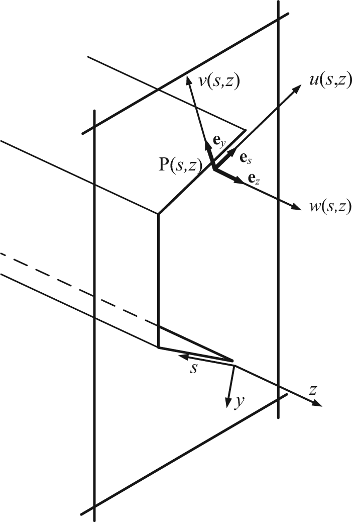
Displacement field.
The displacement field at a point
where a comma denotes differentiation with respect the following variable. The corresponding infinitesimal strains,
According to the semi-variational approach, the displacement components are expressed as a linear combination of several known deformation modes
where a dash denotes differentiation with respect the (sole) independent variable, and
Substituting Equations (4) into Equations (3), the strain field can be rewritten as
Assuming a linear elastic law, the (membrane and flexural) stresses
where
The weak formulation of the elasticity problem is derived by means of the Principle of Virtual Work. This can be expressed, assuming external forces to be constant (or averaged) over the plate thickness, as
where
with the corresponding boundary condition terms applied at
Equations (9) and (10) are here referred as GBT non-conventional equations. The former are a set of coupled differential equations in the amplitude functions
with superscripts
In summary, GBT requires two different steps to be carried out: (a) a cross-section analysis, in which a suitable set of deformation modes (described by
3. Dynamic models for cross-section analysis
The fundamental step of the GBT relies on an adequate selection of the deformation modes. The analysis should capture the beam response in the most accurate way, while including the smallest number of modes and minimizing the complexity of the beam model.
According to the spirit of the semi-variational methods, and similar to what is usually done in applying the Ritz–Galerkin variational methods, it seems quite natural to assume for the deformation modes of the TWB the eigenfunctions of one or more linear eigenvalue problems defined on the 1D domain
In this context, a ‘complete dynamic approach’ is proposed, leading to a GBT-D version of the classical GBT analysis. A segment of TWB of length
In-plane oscillations, in which all points move transversally to the axis (Figure 2(b)). Since
Out-of-plane (or warping) oscillations, in which all points move parallel to the
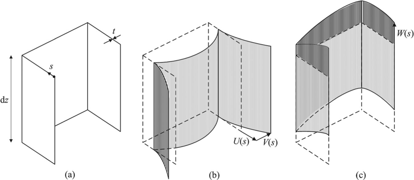
Free oscillations of a segment of thin-walled beam: (a) undeformed body; (b) in-plane oscillations; (c) warping oscillations.
The previous two problems are governed by a set of uncoupled 1D differential equations referred to in the following as the PEP and the WEP, respectively. These are now outlined below separately for clarity.
3.1 The Planar Eigenvalue Problem
3.1.1 The boundary value problem
The PEP is governed by the well-known equations for axial and transverse vibrations of a beam, which are expressed as
where
Equations (13) represent the field equations applicable to each of the
where
Since the frame is unconstrained, the problem admits the triple eigenvalue
3.1.2 The discretized problem
Although the continuous problem (Equations (13) plus boundary conditions) is in principle simple and suitable for a matrix formulation (e.g. see [44]), its discrete version is often preferred in the literature. In this approach, indeed, simpler polynomial functions are used in place of the circular and hyperbolic functions of Equations (14); moreover, as discussed in [44], inextensibility conditions are easier to implement.
The discretization is carried out by subdividing the frame into FEs, obtained by interposing additional nodes between the natural ones. By taking
where
3.1.3 The inextensional and extensional planar modes
Since the matrices
The inextensibility of the
where
are
The inextensional eigenvectors span a
Any vector
where
are
3.2 The Warping Eigenvalue Problem
3.2.1 The boundary value problem
The WEP governs the free oscillations of a pure shear beam. This is an internally constrained Timoshenko beam, in which cross-section rotations are prevented, so that they are only permitted to slide orthogonally to the axis. Therefore, the shear
which is formally identical to Equation (13), with
so that there are
Since the shear beam is free at the ends, it admits the (simple) zero eigenvalue
It is also worth noticing that there is no need to subdivide the domain
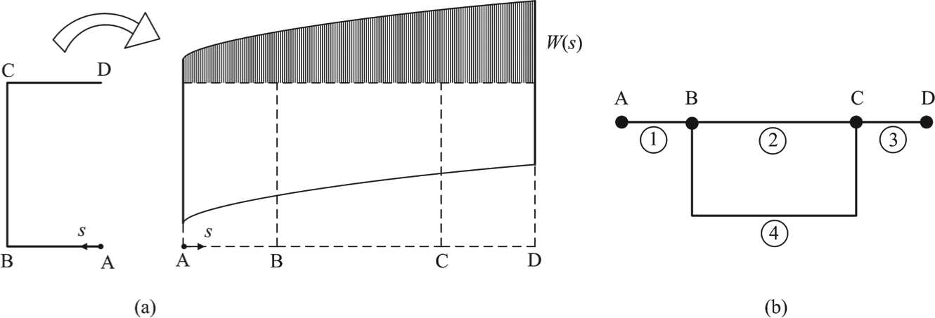
Warping Eigenvalue Problem for: (a) unbranched, constant thickness cross-sections; (b) partially closed cross-sections
3.2.2 The discretized problem
The WEP (Equation (21) and relevant boundary conditions) can, of course, be discretized, although it turns out to be much simpler than the PEP. By using the same discretization adopted for this latter, that is,
where
3.3 Conventional and non-conventional modes
The previous analysis led to determination of three sets of deformation modes: (a) inextensional planar modes
For the previous reasons, aimed to build-up a set of deformation modes which, even if taken in a small number, is able to capture the main behaviour of the beam, it is convenient to supplement the inextensional modes by warping components
given the planar displacement field
In summary, the basis of
4. Member analysis of simply supported thin-walled beams
The member analysis of TWBs is carried out solving the GBT equations (9) and (10). These are a system of differential equations and boundary conditions, often solved in the literature by means of the finite element method (FEM), for example [47]. Such an approach would require a convergence analysis to be performed to estimate possible errors induced for different levels of discretization. This aspect of the problem is outside the scope of this paper, where attention is instead focused on the section analysis. Therefore, it is preferred here to consider special boundary conditions that permit an exact solution of GBT equations.
Based on the above, a TWB is considered and assumed to be simply supported, restrained to torsion and free to warp at the ends. Geometric boundary conditions require
with
Assuming that no forces
with
Substitution of Equations (24) into Equations (9) leads to the following
where
Once
5. Numerical results
The accuracy of the GBT-D formulation is checked with a benchmark membrane problem, for which an analytical solution can be derived considering the case of a flat plate, loaded by in-plane forces acting at longitudinal edges. This is followed by the results calculated for two numerical examples to highlight the ease of use of the proposed approach for the analysis of an open-branched section and partially closed one. In all these problems, the role of the shear and extensional modes on the overall response of the beam is investigated and discussed.
5.1 Benchmark membrane problem of a flat plate
A rectangular flat plate of dimensions
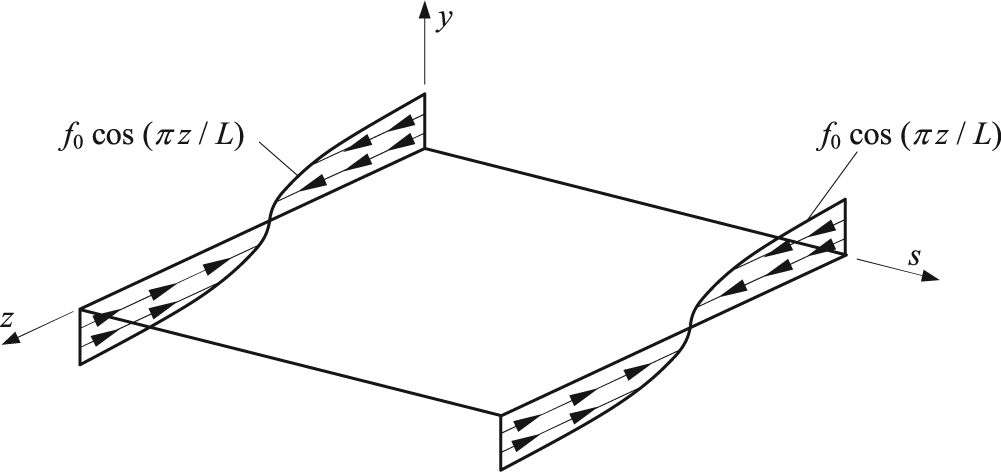
Layout of the flat plate subjected to longitudinal harmonic loads.
For the purpose of the numerical examples, both width and length of the plate are taken equal to 100 mm and the thickness equal to 1 mm. The plate width is discretized with 20 FEs. The material properties include an elastic modulus of 200 GPa and a zero Poisson ratio. The maximum amplitude of the external load
The PEP is first solved in the inextensional space (Equation (16)), leading to modes having
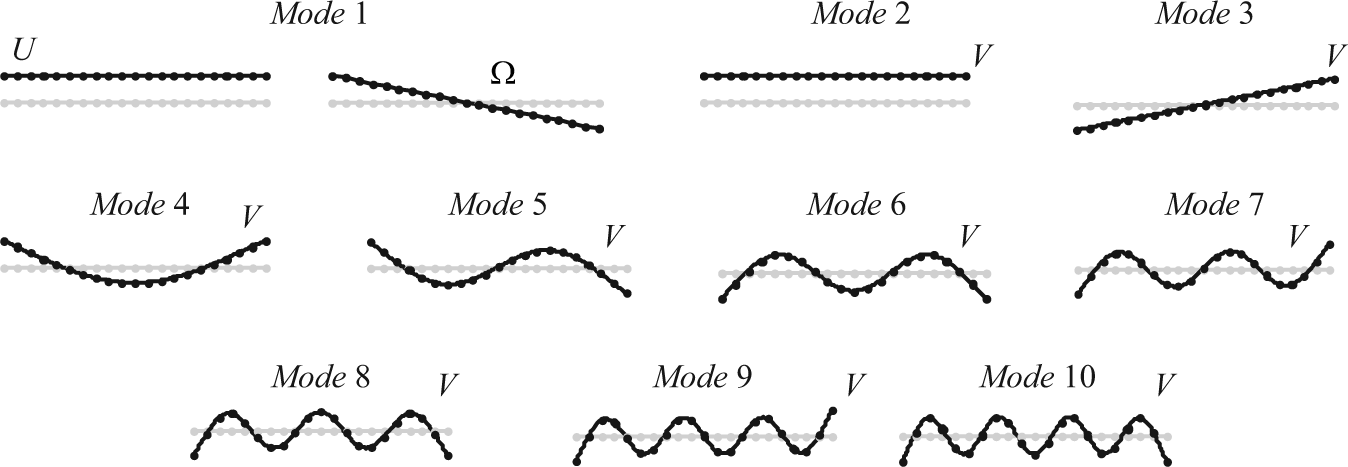
Conventional deformation modes (diagrams in U and Ω).
Successively, the PEP is solved in the extensional subspace (Equation (19)), and deformation modes of purely tangential type
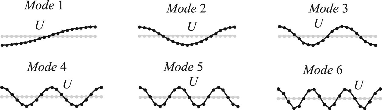
Extension deformation modes (diagrams in U).
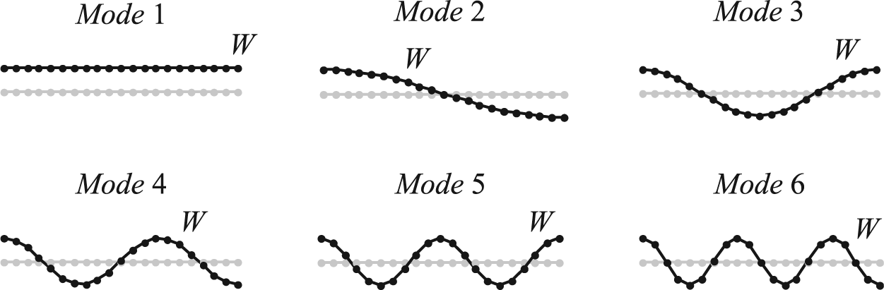
Shear deformation modes (diagrams in W).
The numerical results presented in the following are calculated considering different subsets of the modes previously introduced to evaluate how these influence the accuracy of the solution. In particular, these subsets consist of (a) conventional modes; (b) conventional and shear modes; (c) all modes (conventional, shear and extensional modes). In all cases, all the modes of the subsets obtained from the cross-sectional analysis are used (not only those displayed in Figures 5–7). Two additional solutions are also considered for comparative purposes: (d) FE results obtained with the commercial software Abaqus [48] (in which suitable material and element constraints are introduced), and (e) the analytical solution presented in Appendix D. The Abaqus model is developed with shell elements S4R and with the condition of inextensibility enforced by requiring that no displacements occur in the s direction. A nil Poisson ratio is specified, to reflect the typical GBT assumption (Equation (6)) in which the two membrane normal stresses are not coupled.
Figures 8 reports results (warping, longitudinal and shear stresses evaluated at
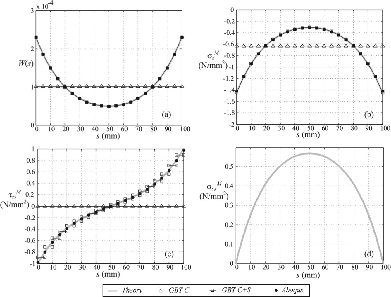
Results obtained for the flat plate section enforcing the transverse inextensibility of the cross-section: (a) warping distribution (z = 0); (b) longitudinal stresses
As a final comment, the variation over the width of the section of the normal stress well depicts the occurrence of shear-lag. This, however, is significant because the length-to-width ratio
The relevant results (warping, longitudinal and transverse normal stresses, tangential stresses, evaluated at
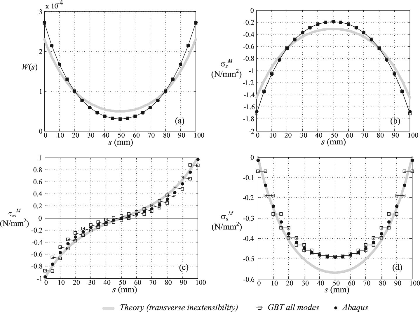
Results obtained for the flat plate section including the transverse extensibility of the cross-section in the analysis: (a) warping distribution (z = 0); (b) longitudinal stresses
5.2 Numerical examples: T-section and box girder
The GBT-D is applied in this section to the analysis of two simply supported TWBs, that is, a T-section beam and a box girder, to better outline its ease of use and highlight the role of the non-conventional modes when considering the accuracy of the solution.
5.2.1 T-section beam
The geometric layout of the TWB considered in this example is depicted in Figure 10. The elastic modulus is 200 GPa and the Poisson ratio 0.3. The loads (forces per unit length) act in the symmetry plane, and are applied to the top flange; their expressions are:
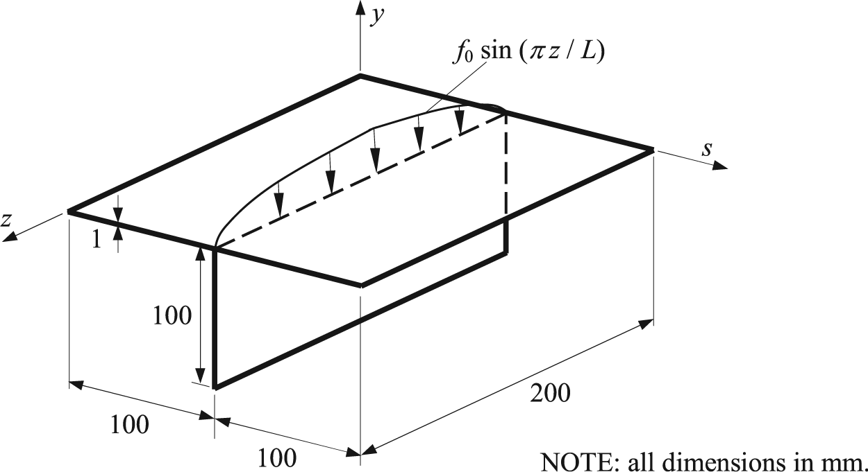
Layout of the T-section and loading arrangement.
The deformation modes, obtained by discretizing each of the three plates in 10 FEs, are illustrated in Figure 11 (where the U- and V-components are displayed by the final position of the nodes, while the W-components are diagrammed). The deformation modes consist of: (a) conventional modes (Figure 11(a)); (b) extensional modes (Figure 11(b)); and (c) shear modes (Figure 11(c)), which include the uniform axial extension mode.
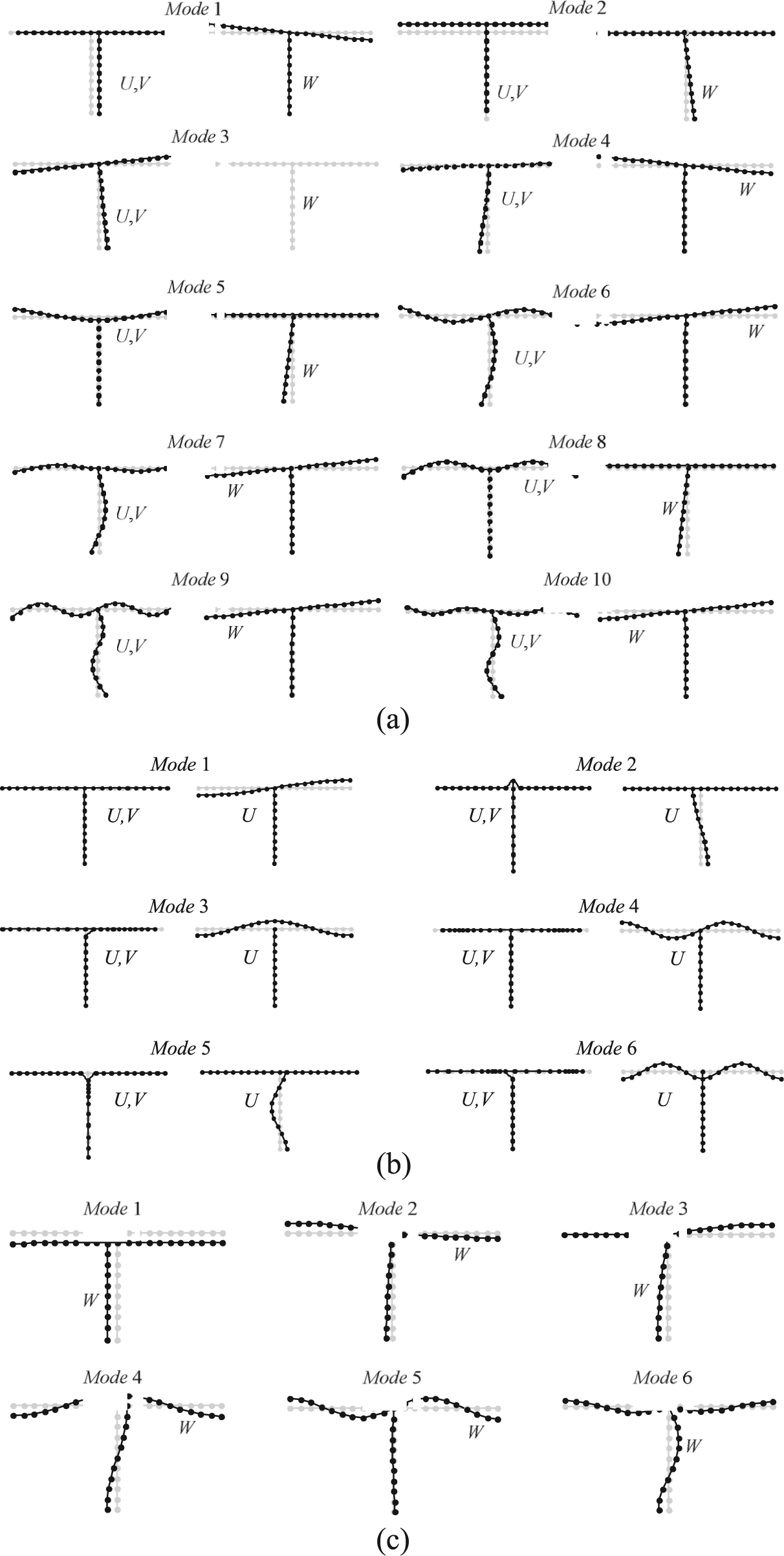
First rigid and deformation modes for the T-section: (a) conventional modes (diagrams in W); (b) extension modes (diagrams in U alone); and (c) shear modes (diagrams).
Results concerning the member analysis are reported in Figure 12, where displacement and stresses are plotted at the abscissa where they attain the maximum values (i.e. at
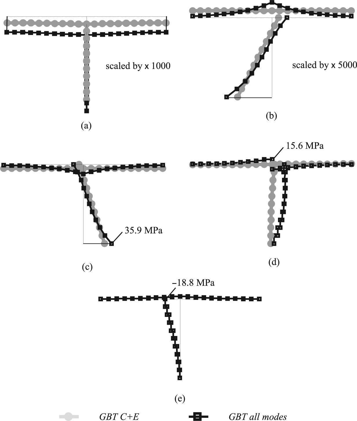
Results calculated for the T-section: (a) in-plane displacements (z = L/2); (b) warping displacements (z = 0,L); (c) longitudinal stresses
5.2.2 Box girder
A box girder (Figure 13) is considered to outline the ability of GBT-D to deal with partially closed sections. The applied load consists of an in-plane longitudinal force (per unit area),
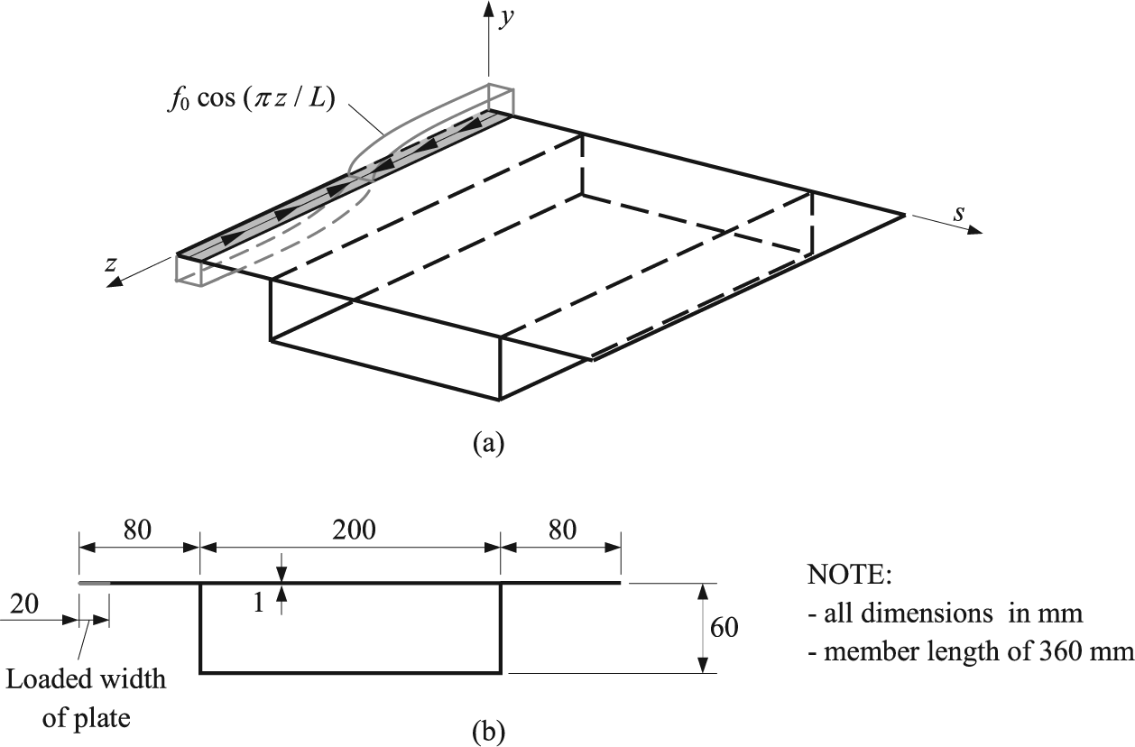
Layout of the box girder and loading arrangement: (a) layout of member and loading arrangement; (b) cross-sectional geometry.
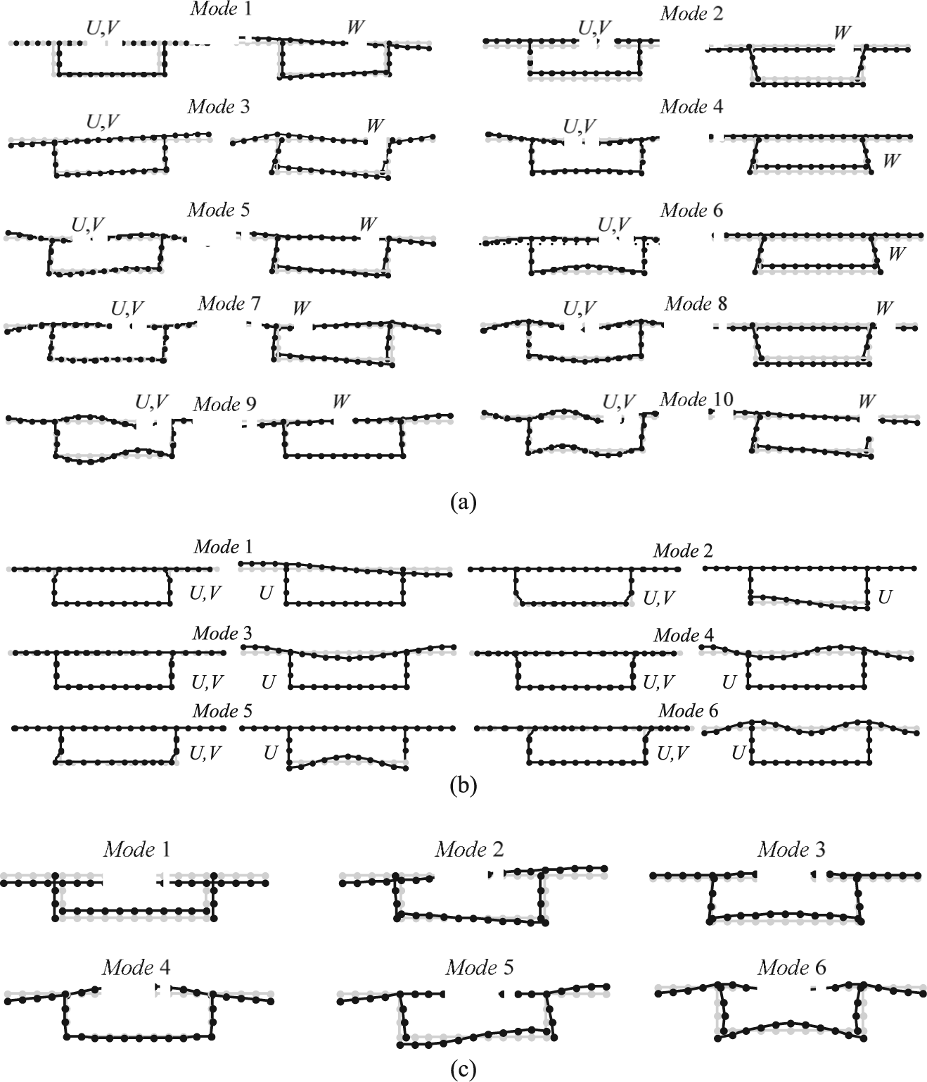
First rigid and deformation modes for the box girder: (a) conventional modes (diagrams in W); (b) extension modes (diagrams in U alone); and (c) shear modes (diagrams).
Similar to the T-section, a comparison between analyses with all modes and no shear modes is presented in Figure 15. These results confirm the need to account for the shearing deformation in order to accurately predict the structural response in terms of both in-plane and warping displacements (Figures 15(a) and (b)), as well as stresses (Figures 15(c)–(e)). This kind of response is particularly important for short members, such as those considered here, for which the length is comparable to the cross-sectional width.
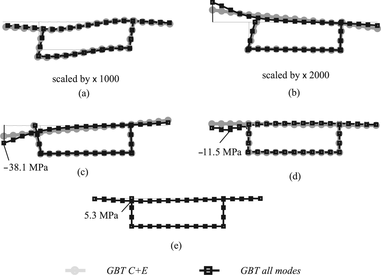
Results calculated for the box girder: (a) in-plane displacements (z = L/2); (b) warping displacements (z = 0,L); (c) longitudinal stresses
6. Conclusions
A new approach to the cross-section analysis of TWBs, to be performed in the framework of the GBT, has been proposed. It is based on evaluation of the dynamic eigenmodes of beam systems, and therefore named GBT-D. The method permits one to replace the sets of (quite involved) elastic analyses required in the classical approach, by simpler eigenmode analyses. The method calls for the following steps to be performed.
Solving the eigenvalue problem for an inextensional frame of planar beam, having the shape of the middle line of the TWB. Supplementing the inextensional planar modes so obtained by warping displacements that assure (a) shear-indeformability of open branches, and (b) constant shear-stress flow along closed loops; these modes are called conventional.
Solving the eigenvalue problem for an extensional planar frame, of the same shape, under the constraint that modes are orthogonal to the inextensional ones; these planar modes are called extensional.
Solving the eigenvalue problem for a planar shear beam, supplying purely warping modes for the TWB; these are named shear modes.
Performing a member analysis, aimed to solve GBT equations in the unknown amplitudes of conventional, extensional and shear deformation modes.
A benchmark membrane problem has been considered, for which an analytical solution can be obtained under inextensibility conditions. It has been shown that the GBT-D analysis is able to accurately reproduce the exact solution when the shear modes, in addition to the conventional, are taken into account. These, of course, are important when shear-lag effects play an important role in describing the structural response, as is the case for short TWBs. Extensional modes are also significant when the inextensibility condition is released, as shown by the comparisons carried out against FE results. Two additional numerical examples have been presented to highlight the efficiency of GBT-D in predicting the response of open and partially closed TWBs. Although similar results can be obtained with refined FE models (for example, by using shell elements), it is in the opinion of the authors that the GBT technique improves the interpretation of the results, and opens the way to the study of reduced-order models. Therefore, the GBT-D is regarded as a simple and efficient tool for the elastic analysis of TWBs.
Footnotes
Appendix A: Stiffness and mass element matrices
The element matrices used in this study for the two-node planar Euler–Bernoulli beam, based on linear and cubic interpolation functions for the axial and transverse displacements, respectively, and relying on the consistent mass approach, are defined as
where
The stiffness (
Appendix B: Constrained algebraic eigenvalue problems
The constrained dynamic eigenvalue problem can be expressed as
where the first equation is the Virtual Work Principle and the second equation expresses a linear constraint for
where
If the constraints express the inextensibility of a planar frame (inextensional PEP), then
In the case the constraints express orthogonality of
Appendix C: Warping component of the conventional modes
The warping in the conventional modes is determined by enforcing the membrane shear-strain in each beam element forming the cross-section to be either (a) zero, when dealing with open branches, or (b) equal to a constant shear flow, when considering closed loops included in the cross-section. For the
Considering that
If the beam possesses an open profile, then
In the presence of closed loops in
where
In summary, the system of equations to be solved consists of one equation for each element, either of type (34) if the element belongs to an open branch, or of type (35) if it belongs to one or more loops. An additional equation is included, which enforces the warping average over the entire cross-section to be nil. The system is then solved for the unknowns, which include the nodal values of warping
Appendix D: Closed-form solution for the benchmark membrane problem of a flat plate
The closed-form solution describing the response of the flat plate depicted in Figure 4 is derived in this section. By assuming that the plate is inextensible along the transverse
where the field equation governs equilibrium in the
Considering external loads with harmonic distributions, the expression for the warping distribution can be obtained with a separation of variable technique as
which, when substituted in Equations (37), leads to
The solution of Equations (39) is then calculated using
with
Finally, the distribution of the reactive stresses
Acknowledgements
The contributions of the first and third authors were partially supported by the Italian Ministry of Education, Universities and Research (MIUR), through the PRIN funded program ‘Dynamics, Stability and Control of Flexible Structures’ (grant number 2010MBJK5B). The work of the second author was supported by the Australian Research Council through its Discovery Projects funding scheme (grant number DP1096454).
Conflict of interest
None declared.