Localized standing waves in a hyperelastic membrane tube and their stabilization by a mean flow

Abstract

We first give a complete analysis of the dispersion relation for travelling waves propagating in a pre-stressed hyperelastic membrane tube containing a uniform flow. We present an exact formula for the so-called pulse wave velocity, and demonstrate that as any pre-stress parameter is increased gradually, localized bulging would always occur before a superimposed small-amplitude travelling wave starts to grow exponentially. We then study the stability of weakly and fully nonlinear localized bulging solutions that may exist in such a fluid-filled hyperelastic membrane tube. Previous studies have shown that such localized standing waves are unstable under pressure control in the absence of a mean-flow, whether the fluid inertia is taken into account or not. Stability of such localized aneurysm-type solutions is desired when aneurysm formation in human arteries is modelled as a bifurcation phenomenon. It is shown that in the near-critical regime axisymmetric perturbations are governed by the Korteweg–de Vries equation, and so the associated (weakly nonlinear) aneurysm solutions are (orbitally) stable with respect to axisymmetric perturbations. Stability of the fully nonlinear aneurysm solutions are studied numerically using the Evans function method. It is found that for each wall–fluid density ratio there exists a critical mean-flow speed above which no axisymmetric unstable modes can be found, which implies that a fully nonlinear aneurysm solution may be completely stabilized by a mean flow.

Keywords

Aneurysm bifurcation stability nonlinear elasticity pulse wave velocity membrane tube localization

1. Introduction

This study is part of our effort to develop a mathematical theory for the initiation of fusiform aneurysms in human arteries. An aneurysm is a pathological, localized dilation of a blood vessel caused by a disease or weakening of the vessel’s wall. Its research has attracted the attention of researchers from a variety of backgrounds due to the high mortality rate associated with aneurysm rupture, and the high impact on the quality of life even if a patient survives an aneurysm rupture [1, 2]. However, there does not seem to exist a quantitative theory concerning aneurysm initiation, although such a theory would be hugely desirable in drug development. Our theory is intended to fill this gap, and it is built on the postulate that initiation of an aneurysm is a bifurcation phenomenon. This theory will ultimately contain the following ingredients:

Assuming that the artery is perfect in the sense that it is circular cylindrical, homogeneous, and is infinitely long, a localized bulge can form when the internal pressure reaches a certain critical value.

When imperfections such as localized wall-weakening are introduced, the bifurcation pressure will fall to within the physiologically possible range, i.e. of the order of 120 mmHg.

The localized bulging configuration is a stable state since otherwise it cannot be observed.

Thus, we assume that aneurysm initiation is entirely mechanical, but we further postulate that once a localized bulge has formed, blood will become trapped, or even clotted, in the sacs of the aneurysm, and it is the latter that will trigger biological responses, such as remodelling, giving rise to the subsequent evolution of the aneurysm shape. The major difference between our theory and the prevalent point of view [3, 4] is that in the latter there is no bifurcation preceding the remodelling process. Points (1) and (2) have been accomplished in our earlier papers [5 –7], although whether bifurcation can take place or not was found to be very sensitive to the arterial models used, and there is currently still much uncertainty about realistic material models for live arteries. In order to establish (3), we have recently examined the effect of fluid inertia on the stability properties of localized bulging solutions [8], following on from an earlier work [9] where fluid inertia was neglected. It was found that although fluid inertia would reduce the growth rate of the single unstable mode significantly, it alone cannot stabilize the unstable mode completely. Our next candidate for stabilizing the aneurysm solution is a mean flow, which is the subject of the present paper.

Our research has initially been motivated by the geometrical similarity between a fusiform aneurysm and a localized bulge that would form when a rubber membrane tube was inflated by an internal pressure. The latter problem has been much studied experimentally [10, 11], numerically [12], as well as theoretically [13, 14] by researchers in the finite elasticity and engineering communities because it serves as a paradigm for a variety of problems involving multi-phase deformations. For a long time, however, it was not appreciated that localized bulging was in fact a bifurcation phenomenon. This is probably due to the fact that in the two communities, researchers were preoccupied with bifurcations into periodic patterns, and there was a lack of cross-fertilization between these communities and the centre-manifold reduction community (see, e.g., [15]). It was only recently [5] that the bifurcation nature of localized bulging was clarified. In particular, it was shown in Fu et al. [5] that, contrary to popular belief, localized bulging does not always occur at the limiting pressure associated with uniform inflation.

Our present study is also closely related to studies on solitary waves in fluid-filled hyper-elastic membrane tubes. On the one hand, a static localized bulge can be viewed as a solitary wave that has zero propagation speed, the zero speed being induced by the prestress in the membrane tube. On the other hand, solitary waves may play an important role in interrogating the health state of arteries (e.g. presence of an aneurysm) through signal processing [16, 17]. Solitary waves in a fluid-filled membrane tube were initially studied using a multiple-scale approach [18, 19], but later Epstein and Johnston [20] demonstrated that this approach is not necessary because the reduced governing equations admit two integrals; the evolution equation can be derived by an elementary method. We refer to our previous paper [21] for a review of the relevant literature.

The rest of this paper is divided into six sections as follows. After presenting the governing equations and some constitutive assumptions in the next section, we derive in Section 3 some preparatory results concerning linear travelling waves. In particular, we show that as the internal pressure or mean flow speed is increased, formation of a localized bulge always precedes the so-called normal-mode instability that is signified by exponential growth of a linear travelling wave mode. This is then followed in Section 4 by a characterization of both weakly and fully nonlinear static aneurysm solutions in the presence of a mean flow. In Sections 5 and 6 we discuss stability of the weakly and fully nonlinear aneurysm solutions, respectively. The paper is concluded in Section 7 with further discussions.

2. Problem formulation and constitutive assumptions

We consider axi-symmetric motions of an incompressible, isotropic, hyperelastic, cylindrical membrane tube that has a constant undeformed radius $R$ and a constant undeformed thickness $H$ . The tube is assumed to be infinitely long, and so end conditions are imposed at infinity. In terms of cylindrical polar coordinates $r, θ, z$ the current configuration is described by

r = r (Z, t), θ = Θ, z = z (Z, t),

(1)

where $t$ denotes time, and $Θ, Z$ are cylindrical polar coordinates in the undeformed configuration.

The principal directions of the deformation correspond to the lines of latitude, the meridian and the normal to the deformed surface, and the principal stretches are given by

λ_{1} = \frac{r}{R}, λ_{2} = {(r'^{2} + z'^{2})}^{\frac{1}{2}}, λ_{3} = \frac{h}{H},

(2)

where the indices 1, 2, 3 signify the circumferential, meridional, and normal directions, respectively, a prime represents partial differentiation with respect to $Z$ , and $h$ denotes the deformed thickness.

The principal Cauchy stresses $σ_{1}$ , $σ_{2}$ , $σ_{3}$ in the deformed configuration are given by

σ_{i} = λ_{i} {\hat{W}}_{i} - p, i = 1, 2, 3 (no summation),

(3)

where $\hat{W} = \hat{W} (λ_{1}, λ_{2}, λ_{3})$ is the strain-energy function, ${\hat{W}}_{i} = \partial \hat{W} / \partial λ_{i}$ , and $p$ is the pressure associated with the constraint of incompressibility. Utilizing the incompressibility constraint $λ_{1} λ_{2} λ_{3} = 1$ and the membrane assumption of negligible stress through the thickness direction (i.e. $σ_{3} = 0$ ), we find

σ_{i} = λ_{i} W_{i}, i = 1, 2,

(4)

where $W (λ_{1}, λ_{2}) = \hat{W} (λ_{1}, λ_{2}, λ_{1}^{- 1} λ_{2}^{- 1})$ and $W_{1} = \partial W / \partial λ_{1}$ etc. [22].

For illustrative calculations, we shall use the Gent material model given by

\hat{W} = - \frac{1}{2} μ J_{m} \ln (1 - \frac{λ_{1}^{2} + λ_{2}^{2} + λ_{3}^{2} - 3}{J_{m}}),

(5)

where $μ$ is the ground state shear modulus and $J_{m} > 0$ is a material constant characterizing the maximum stretch of the material. This model was originally proposed by Gent [23] to model rubber and rubber-like materials, its relevance to arterial walls having been discussed by Horgan and Saccomandi [24]. More sophisticated material models for arterial walls are available; see, for instance, Holzaphel and Ogden [25], but we believe that our qualitative stability results should be independent of the material model used.

The equations of motion of the wall are given by [20]

[R σ_{2} \frac{z'}{λ_{2}^{2}}] - Prr' = ρ R \overset{\cdot\cdot}{z}, [R σ_{2} \frac{r'}{λ_{2}^{2}}] - \frac{σ_{1}}{λ_{1}} + Prz' = ρ R \overset{\cdot\cdot}{r},

(6)

where a superimposed dot denotes differentiation with respect to $t$ , $ρ$ is the density of the material, and $P$ denotes the pressure exerted by the fluid on the wall divided by H.

To describe the axisymmetric fluid motion inside the tube we use Eulerian cylindrical polar coordinates $y$ , $θ$ , and $z$ , where $y$ denotes the radial coordinate. Let ${u_{y}, 0, u_{z}}^{T}$ denote the fluid velocity. We also introduce

D = {(y, z) | 0 < y < r (z, t); - \infty < z < \infty}

as the domain inside the deformed tube, and

\partial D = {(y, z) | y = r (z, t); - \infty < z < \infty}

as the boundary of this domain, or the tube wall. We consider the fluid to be inviscid and incompressible. Then the equations of motion of the fluid consist of the continuity equation

\frac{\partial u_{y} y}{\partial y} + y \frac{\partial u_{z}}{\partial z} = 0, (y, z) \in D,

(7)

and Euler’s equations

\begin{matrix} \frac{\partial u_{y}}{\partial t} + u_{y} \frac{\partial u_{y}}{\partial y} + u_{z} \frac{\partial u_{y}}{\partial z} = - \frac{1}{ρ_{f}} \frac{\partial (H \hat{P})}{\partial y}, \\ \frac{\partial u_{z}}{\partial t} + u_{y} \frac{\partial u_{z}}{\partial y} + u_{z} \frac{\partial u_{z}}{\partial z} = - \frac{1}{ρ_{f}} \frac{\partial (H \hat{P})}{\partial z}, (y, z) \in D \end{matrix}

(8)

where $ρ_{f}$ is the fluid density and $H \hat{P}$ is the fluid pressure.

We also need the kinematic condition that each particle of fluid does not pass through the boundary $\partial D$ :

\frac{\partial r}{\partial t} + u_{z} \frac{\partial r}{\partial z} = u_{y}, (y, z) \in \partial D .

(9)

To simplify the boundary-value problem (6) – (9) we adopt the long wave approximation for the equations (7)–(9), and assume that

u_{z} (y, z, t) = v_{f} (z, t) + ζ v_{1} (y, z, t), \hat{P} (y, z, t) = P (z, t) + ζ P_{1} (y, z, t),

(10)

where $ζ = R / L << 1$ , $L$ being a characteristic wavelength, and the $O (ζ)$ terms are assumed to vanish when integrated over the cross-section. The $P$ here can be identified with the $P$ in (6) .

Integrating (7) from $0$ to $r$ and substituting (10) we obtain to zeroth order in $ζ$

u_{y} (r (z, t), z, t) + \frac{r}{2} \frac{\partial v_{f}}{\partial z} = 0,

(11)

which, after the substitution of (9) and (10), can also be written as

\frac{\partial r}{\partial t} + v_{f} \frac{\partial r}{\partial z} + \frac{r}{2} \frac{\partial v_{f}}{\partial z} = 0 .

(12)

The second equation in (8) to zeroth order in $ζ$ gives

\frac{\partial v_{f}}{\partial t} + v_{f} \frac{\partial v_{f}}{\partial z} = - \frac{1}{ρ_{f}} \frac{\partial HP}{\partial z} .

(13)

The equations (12) and (13) were introduced by Demiray [26] as a simple model whereby the conservation of mass and momentum is enforced under the assumptions that the fluid is inviscid and incompressible, $u_{y} \equiv 0$ , and $u_{z}$ is constant throughout the tube cross section.

The connection between the Eulerian longitudinal coordinate $z$ and the Lagrangian coordinate $Z$ is given by (1). For any dependent variable $Ψ$

Ψ' = \frac{\partial Ψ}{\partial z} z', \overset{\cdot}{Ψ} = \frac{\partial Ψ}{\partial z} \overset{\cdot}{z} + \frac{\partial Ψ}{\partial t} .

Therefore, in terms of the Lagrangian coordinate $Z$ equations (12) and (13) assume the form

\overset{\cdot}{r} z' - r' \overset{\cdot}{z} + v_{f} r' + \frac{1}{2} r v_{f}' = 0, ρ_{f} [{\overset{\cdot}{v}}_{f} z' - v_{f}' \overset{\cdot}{z} + v_{f} v_{f}'] + HP' = 0 .

(14)

The equations (6) and (14) constitute the governing equations that determine the dynamics of the fluid and the tube wall.

Before proceeding further, we shall non-dimensionalize the above governing equations using the following scales: $R$ for $Z, z$ and $r$ , $μ$ for the strain-energy function $W$ and Cauchy stresses, $μ / R$ for $P$ , $\sqrt{μ / ρ}$ for $v_{f}$ , and $R \sqrt{ρ / μ}$ for the time. Using the same notation for the scaled variables, we have

[σ_{2} \frac{z'}{λ_{2}^{2}}] - Prr' = \overset{\cdot\cdot}{z}, [σ_{2} \frac{r'}{λ_{2}^{2}}] - \frac{σ_{1}}{λ_{1}} + Prz' = \overset{\cdot\cdot}{r},

(15)

\overset{\cdot}{r} z' - r' \overset{\cdot}{z} + v_{f} r' + \frac{1}{2} r v_{f}' = 0, b_{f} [{\overset{\cdot}{v}}_{f} z' - v_{f}' \overset{\cdot}{z} + v_{f} v_{f}'] + P' = 0,

(16)

where $b_{f}$ , defined by

b_{f} = \frac{ρ_{f} R}{ρ H},

(17)

is a non-dimensional constant characterizing the fluid inertia. We note that $λ_{1}$ is now identical to $r$ .

The governing equations (15) and(16) admit the uniform solution

r = r_{\infty}, z' = λ_{2} = λ_{2 \infty}, v_{f} = v_{f \infty}, P = P_{\infty} \equiv \frac{W_{1} (r_{\infty}, λ_{2 \infty})}{r_{\infty} λ_{2 \infty}},

(18)

where $r_{\infty}, λ_{2 \infty}$ and $v_{f \infty}$ are constants. Corresponding to this uniform solution, the axial force $F$ is given by

\frac{F}{π μ RH} = 2 W_{2} (r_{\infty}, λ_{2 \infty}) - \frac{r_{\infty} W_{1} (r_{\infty}, λ_{2 \infty})}{λ_{2 \infty}} .

(19)

For the case of closed ends and fixed $F$ (assuming in this case that there is no mean flow),(19) defines $λ_{2 \infty}$ as a function of $r_{\infty}$ . It can easily be shown that

\frac{dP}{dv} = \frac{2 (3 β_{0} + β_{1} + 4 γ_{1} - 4 α_{1}) [γ_{1} (β_{1} - β_{0}) - {(α_{1} - β_{0})}^{2}]}{λ_{2 \infty}^{2} {(- 2 α_{1} + β_{0} + β_{1})}^{2}},

(20)

where $v = r_{\infty}^{2} λ_{2 \infty}$ denotes the fractional volume change, and the various constants on the right-hand side are defined by

α_{0} = λ_{2 \infty} W_{2}^{(\infty)}, β_{0} = r_{\infty} W_{1}^{(\infty)}, α_{1} = r_{\infty} λ_{2 \infty} W_{12}^{(\infty)}, β_{1} = r_{\infty}^{2} W_{11}^{(\infty)}, γ_{1} = λ_{2 \infty}^{2} W_{22}^{(\infty)},

where a superscript $(\infty)$ denotes evaluation at the uniform state (18) .

On the other hand, if we fix the pressure $P$ , the right-most equation of(18) then defines $r_{\infty}$ as a function of $λ_{2 \infty}$ , and it can then be shown that

\frac{\partial}{\partial λ_{2 \infty}} (\frac{F}{π μ RH}) = \frac{2}{λ_{2 \infty}^{2} (β_{1} - β_{0})} [γ_{1} (β_{1} - β_{0}) - {(α_{1} - β_{0})}^{2}] .

(21)

We observe that the same factor $γ_{1} (β_{1} - β_{0}) - {(α_{1} - β_{0})}^{2}$ appears in both (20) and (21), and that this factor also appears in the conditions

α_{0} > 0, γ_{1} > 0, β_{1} γ_{1} - α_{1}^{2} > 0, (β_{1} - β_{0}) γ_{1} - {(α_{1} - β_{0})}^{2} > 0,

(22)

which are necessary and sufficient for stability of the uniformly inflated state (18) under pressure control with free ends and $v_{f}$ $= 0$ [27]. It is also known that this expression equal to zero is the condition for a localized bulge to bifurcate from the uniform state (18) in the absence of a mean flow [5, 8]. Throughout this paper we assume that (22) are satisfied. We also observe that the second and fourth equations in (22) imply that $(β_{1} - β_{0}) > 0$ .

Equation (20) shows that for the case of closed ends and fixed $F$ , the first pressure turning point corresponds to the onset of localized bulging, as has been observed experimentally [10, 11]. However, human arteries have the important property that pressure fluctuations can be accommodated by very little extra axial stretch. Thus, it is appropriate to assume in the associated analysis that the axial stretch $λ_{2 \infty}$ is fixed. In this case a variable axial force $F$ needs to be applied as $P$ varies, and onset of localized bulging does not correspond to the first turning point in the pressure versus volume curve [5] (although the bifurcation condition takes the same mathematical form in both cases). In fact, localized bulging always takes place before the turning point is reached if the latter turning point exists, and can take place even if the latter turning point does not exist at all. In other words, contrary to popular belief, the existence of the so-called limit point instability is not a necessary condition for localized bulging to occur. Instead, from (21) we see that the necessary physical condition is that the axial force versus axial stretch at a fixed pressure has a turning point. This fact does not seem to have previously been noted in the literature. With application to aneurysm formation in mind, we shall from now on assume that $λ_{2 \infty}$ is prescribed, and view $r_{\infty}$ and $v_{f \infty}$ as the control parameters that can be varied. We note that under the assumptions (22), pressure $P$ is a monotonically increasing function of $r_{\infty}$ , and so equally we could use pressure as one of the control parameters.

3. Dispersion relation for linear travelling waves

Later in our analysis we shall need to refer to the dispersion relation for small-amplitude travelling waves superimposed on the uniform state (18) . Assuming that the small-amplitude perturbations are proportional to

\exp (i \frac{λ_{2 \infty}}{r_{\infty}} k (Z - \frac{c t}{λ_{2 \infty}})),

then the scaled wavenumber $k$ and wave speed $c$ satisfy the dispersion relation [21]

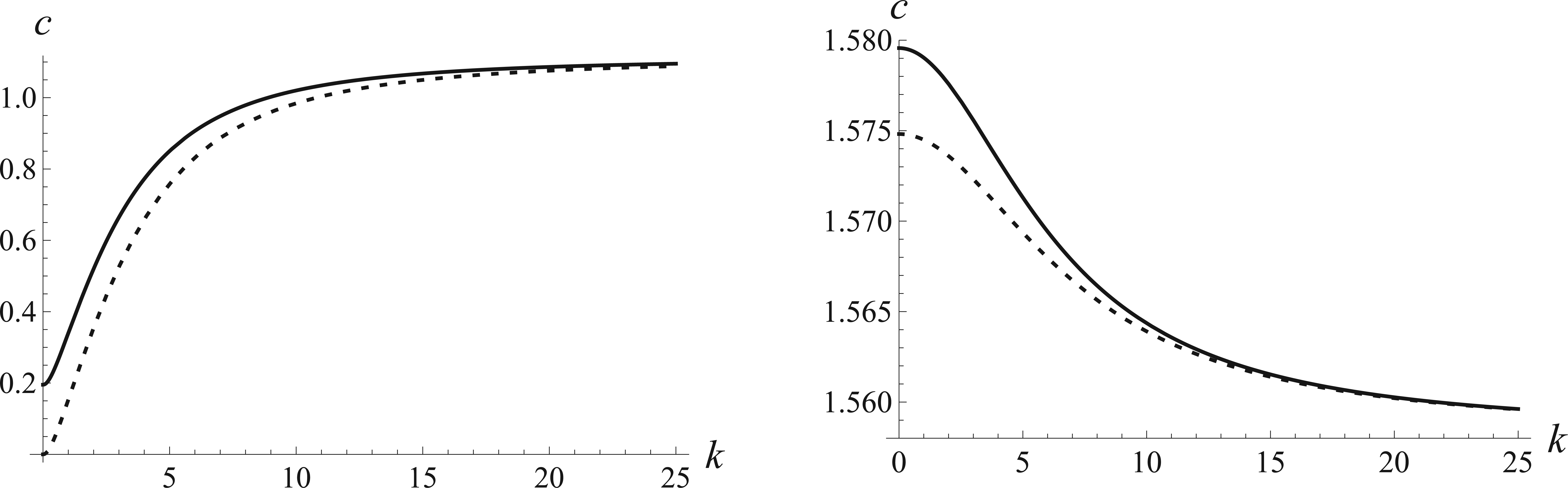
\begin{matrix} (k^{2} m + 2) c^{4} - 4 v_{f \infty} c^{3} - (m α_{0} k^{2} + m γ_{1} k^{2} - 2 v_{f \infty}^{2} - m β_{0} + m β_{1} + 2 γ_{1}) c^{2} \\ + 4 v_{f \infty} γ_{1} c - 2 v_{f \infty}^{2} γ_{1} + m γ_{1} (k^{2} α_{0} + β_{1} - β_{0}) - m {(α_{1} - β_{0})}^{2} = 0, \end{matrix}

(23)

where $m = 1 / (b_{f} r_{\infty}^{2} λ_{2 \infty})$ . We note that the notations here are the same as those in [21] except that the $c$ and $v_{f \infty}$ here correspond to $\sqrt{m} c$ and $\sqrt{m} v_{f \infty}$ there. In the limit $k \to \infty$ , the four branches of the dispersion relation tend to $c = \pm \sqrt{α_{0}}$ and $c = \pm \sqrt{γ_{1}}$ , respectively, which are independent of $v_{f \infty}$ and $m$ . Furthermore, when $c = \pm \sqrt{γ_{1}}$ , the left-hand side of (23) reduces to $- m {(α_{1} - β_{0})}^{2}$ , which is in general non-zero (in particular it is non-zero in the stress-free configuration where $β_{0} \equiv 0$ ). Thus, we deduce that the four branches will never cross the asymptotic lines $c = \pm \sqrt{γ_{1}}$ . Figure 1 shows the four branches of the dispersion relation for a typical case in which the four wave speeds are real for all $k$ but with one speed vanishing at $k = 0$ . Note that to show enough details we have multiplied the negative wave speeds by $- 1$ (shown as dotted lines).

Figure 1.

The four branches of (23) when $λ_{2 \infty} = 1.2$ , $r_{\infty} = 1.634$ , $b_{f} = 3.47$ , and $v_{f}$ $= 0.1$ . Left: the two inner branches; right: the two outer branches. The speed corresponding each of the dotted curves is minus the actual speed, and so when $v_{f}$ $= 0$ the two curves in each figure would coincide with each other.

Before analysing (23) in the general case further, we first consider the double limit $ρ_{f} \to 0$ and $v_{f}$ $\to 0$ under which the dispersion relation can be solved exactly to give

c^{2} = \frac{1}{2} (B \pm \sqrt{B^{2} - 4 k^{- 2} C}) = \frac{1}{2} (B \pm \sqrt{{[k^{- 2} (β_{0} - β_{1}) - α_{0} + γ_{1}]}^{2} + 4 k^{- 2} {(α_{1} - β_{0})}^{2}}),

where

B = k^{- 2} (β_{1} - β_{0}) + α_{0} + γ_{1}, C = γ_{1} (β_{1} - β_{0}) - {(α_{1} - β_{0})}^{2} + α_{0} γ_{1} k^{2} .

Thus, the stability conditions (22) guarantee that the four wave speeds are real for all $k$ , and in the long wavelength limit $k \to 0$ the four roots have the asymptotic behaviour

c^{2} = \frac{β_{1} - β_{0}}{k^{2}} + O (1), or \frac{1}{2 (β_{1} - β_{0})} [(β_{1} - β_{0}) γ_{1} - {(α_{1} - β_{0})}^{2}] + O (k^{2}) .

(24)

It is seen that the bifurcation condition for localized bulging corresponds to two of the four wave speeds vanishing at the same time in the long wave length limit. This is also true even if $ρ_{f} \neq 0$ , and is the reason why the evolution of near-critical modes is governed by the Boussinesq equation [8, 9].

Suppose now that $ρ_{f}$ and $v_{f \infty}$ are both non-zero. We first examine the behaviour of the dispersion relation (23) at $k = 0$ where it reduces to

\begin{matrix} 2 c^{4} - 4 v_{f \infty} c^{3} - (- 2 v_{f \infty}^{2} - m β_{0} + m β_{1} + 2 γ_{1}) c^{2} \\ + 4 v_{f \infty} γ_{1} c - 2 v_{f \infty}^{2} γ_{1} + m γ_{1} (β_{1} - β_{0}) - m {(α_{1} - β_{0})}^{2} = 0 . \end{matrix}

(25)

When $v_{f}$ $= 0$ , the above equation becomes a bi-quadratic and the roots can be written as

4 c^{2} = 2 γ_{1} + m (β_{1} - β_{0}) \pm \sqrt{{[2 γ_{1} - m (β_{1} - β_{0})]}^{2} + 8 m {(α_{1} - β_{0})}^{2}},

(26)

so that the four roots are all real. It can easily be shown that these two expressions satisfy $c^{2} < γ_{1}$ and $c^{2} > γ_{1}$ , respectively. The expression satisfying $c^{2} < γ_{1}$ would recover the Moens–Korteweg formula $c_{0} = \sqrt{3 μ H / (2 ρ_{f} R)}$ for the pulse wave velocity in arteries if we took the further limit $r_{\infty} \to 1$ , $λ_{2 \infty} \to 1$ , $ρ \to 0$ . This velocity value and its various improved forms [28] are often used in the medical community as a measure of the arterial stiffness and a risk factor for cardiovascular morbidity and mortality [29].

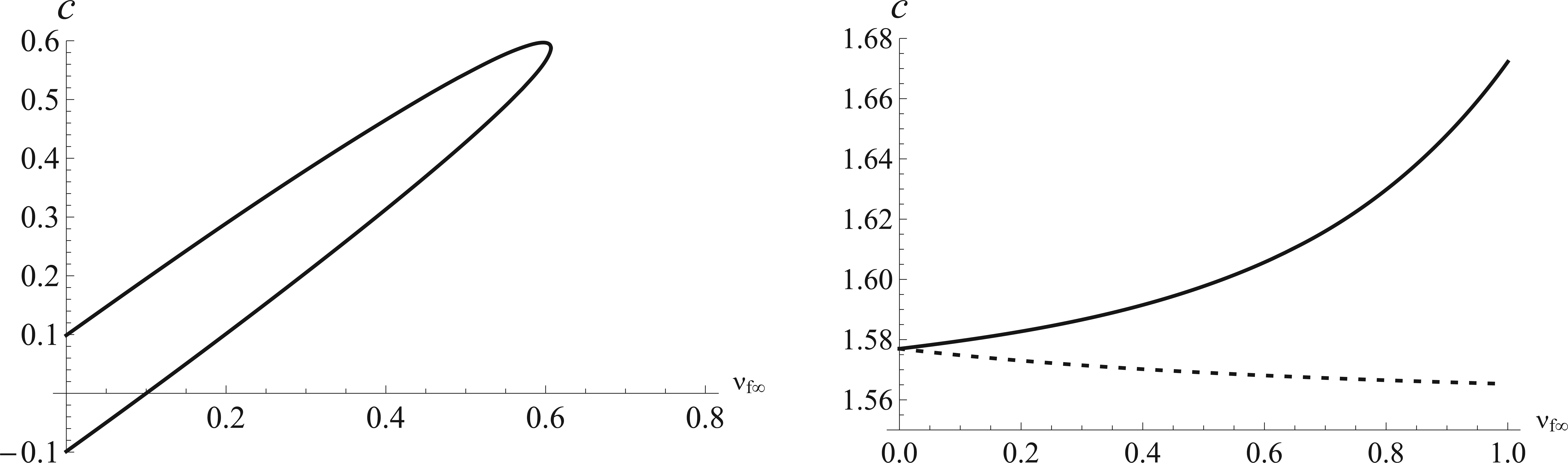
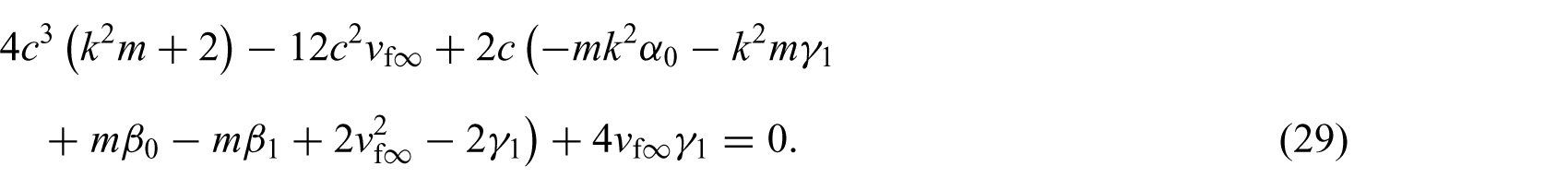
Figure 2 shows the fate of the four roots given by (26) as $v_{f \infty}$ is increased from $0$ . It is seen that for the case considered, the two inner branches coalesce at $v_{f}$ $= 0.6066$ , beyond which they do not exist any more (and the corresponding speeds then become complex), while the other two branches exist for all values of $v_{f \infty}$ . Since the two coalescing branches are on opposite sides of the $v_{f \infty}$ -axis when $v_{f}$ $= 0$ , one of these two branches mustcross the $v_{f \infty}$ -axis first before it coalesces with the other branch. The crossing takes places when zero becomes a root of (25), that is when

γ_{1} (β_{1} - β_{0}) - {(α_{1} - β_{0})}^{2} - 2 v_{f \infty}^{2} γ_{1} / m = 0 .

(27)

Figure 2.

Variation of the four roots of (25) with respect to $v_{f \infty}$ when $λ_{2 \infty} = 1.2$ , $r_{\infty} = 1.634$ , $b_{f} = 3.47$ . Left: the two inner branches; right: the two outer branches (here the speed corresponding to the dotted line is minus the actual speed). The two inner branches exist only for $v_{f}$ $< 0.6066$ .

It will be shown later that this equation is in fact the bifurcation condition for the initiation of a localized bulge in the presence of a mean flow. Thus, root coalescing at $k = 0$ , and hence any wave speed becoming complex, always takes place after the bifurcation condition (27) has been satisfied. Note also that root coalescing can only take place between the two inner branches because otherwise the asymptotic lines $c = \pm \sqrt{γ_{1}}$ will need to be crossed.

The critical value of $v_{f \infty}$ at which two roots coalesce is determined by

p^{3} + q^{2} = 0,

(28)

where

\begin{matrix} p = - m^{2} β_{1}^{2} + 2 m β_{0} (m β_{1} - 2 v_{f \infty}^{2} + 14 γ_{1}) + 4 {mv}_{f \infty}^{2} β_{1} - 48 m α_{1} β_{0} \\ + 24 m α_{1}^{2} - 28 m β_{1} γ_{1} - (m - 24) m β_{0}^{2} - 4 v_{f \infty}^{4} + 8 v_{f \infty}^{2} γ_{1} - 4 γ_{1}^{2}, \end{matrix}

\begin{matrix} q = - 9 (m β_{0} - m β_{1} - v_{f \infty}^{2} - 2 γ_{1}) (m^{2} β_{1}^{2} - 2 m β_{0} (m β_{1} + 2 v_{f \infty}^{2} - 2 γ_{1}) + 4 {mv}_{f \infty}^{2} β_{1} \\ - 16 m α_{1} β_{0} + 8 m α_{1}^{2} - 4 m β_{1} γ_{1} + m (m + 8) β_{0}^{2} + 8 v_{f \infty}^{2} γ_{1} + 4 γ_{1}^{2}) \\ - 8 {(- m β_{0} + m β_{1} + v_{f \infty}^{2} + 2 γ_{1})}^{3} - 27 v_{f \infty}^{2} {(m β_{0} - m β_{1} + 2 γ_{1})}^{2} . \end{matrix}

Equation (28) is obtained from an elementary analysis of the roots of the quartic (25) [30]. The left-hand side of (28) is a positive multiple of the discriminant of a certain resolvent cubic and it must necessarily be negative when $v_{f}$ $= 0$ (which follows from the fact that (25) has four real roots), and the critical value of $v_{f \infty}$ is the first zero of $p^{3} + q^{2}$ as $v_{f \infty}$ is increased from zero.

We next consider the behaviour of the dispersion curve when $k \neq 0$ . We recall that in the limit $k \to \infty$ the four wave speeds tend to $\pm \sqrt{α_{0}}$ , $\pm \sqrt{γ_{1}}$ , which are all real under the assumptions (22), and are independent of the flow properties $v_{f \infty}$ and $m$ . As $v_{f \infty}$ is increased from zero, the behaviour of the four branches in the large $k$ regime is little changed, but in the small $k$ regime the two middle branches may coalesce (see Figure 3). If coalescing takes place at $k = k_{t}$ , say, then two of the wave speeds are complex for $k < k_{t}$ . The coalescing point $k = k_{t}$ has the property that $dc / dk \to \infty$ , or equivalently by differentiating (23) with respect to $k$ implicitly and then setting the coefficient of $dc / dk$ to zero,

\begin{matrix} 4 c^{3} (k^{2} m + 2) - 12 c^{2} v_{f \infty} + 2 c (- m k^{2} α_{0} - k^{2} m γ_{1} \\ + m β_{0} - m β_{1} + 2 v_{f \infty}^{2} - 2 γ_{1}) + 4 v_{f \infty} γ_{1} = 0 . \end{matrix}

(29)

Figure 3.

A typical dispersion curve when a pair of complex roots exist for small enough $k$ , when $λ_{2 \infty} = 1.2$ , $r_{\infty} = 1.634$ , $b_{f} = 3.47$ and $v_{f}$ $= 0.9$ .

The resultant of (23) and (29) equal to zero then defines $k_{t}$ as a function of $v_{f \infty}$ . The minimum of $v_{f \infty}$ is clearly attained when $k_{t} = 0$ , in which case the above-defined resultant equal to zero is expected to be equivalent to (28). We have verified that this is indeed the case. In view of these results and the earlier results for $k = 0$ , we may conclude that if we denote by $r_{cr}$ the first zero of (27) for each fixed $v_{f \infty}$ , then for $r_{\infty} < r_{cr}$ , root coalescing cannot occur and the four roots of (23) are all real for all values of $k$ .

If on the other hand we fix $r_{\infty}$ and increase $v_{f \infty}$ beyond the first root of (28), small-amplitude travelling waves will grow exponentially (assuming that localized bulging is suppressed), which corresponds to a more serious instability than the localized bulging under consideration. However, our analysis above shows that this more serious instability is always preceded by localized bulging.

4. Weakly and fully nonlinear bulging solutions

With the dispersion relation well understood, we are now in a position to characterize weakly and fully nonlinear localizedstanding wave solutions. We start by looking for a general localizedtravelling wave solution for which the dependence on $Z$ and $t$ is through $Z - ct / λ_{2 \infty}$ , where $c$ now denotes the wave speed of the fully nonlinear wave. Localization means that as $Z - ct / λ_{2 \infty} \to \pm \infty$ , the fluid-filled tube is in a uniform state given by (18). From now on, we use $Z$ to mean $Z - ct / λ_{2 \infty}$ . Standing wave solutions will be recovered by setting $c = 0$ .

It can easily be shown [20] that the fluid equations (16) in this case can be integrated to yield

P = P_{\infty} + v_{f 0} (1 - \frac{r_{\infty}^{4}}{r^{4}}), v_{f} = \frac{v_{f \infty} r_{\infty}^{2}}{r^{2}},

(30)

where the constant $v_{f 0}$ is defined by

v_{f 0} = \frac{1}{2} b_{f} {(v_{f \infty} - c)}^{2} .

It is also known that the two equations in(15) together with(30) have two integrals, that can be obtained by integrating the first equation in(15), and $z'$ times the first equation in(15) added to $r'$ times the second equation in(15), respectively. They are given by

W - λ_{2} W_{2} + c^{2} λ_{2}^{2} / (2 λ_{2 \infty}^{2}) = C_{1},

(31)

W_{2} z' / λ_{2} - P^{*} r^{2} / 2 - c^{2} z' / λ_{2 \infty}^{2} = C_{2},

(32)

where a prime again denotes differentiation with respect to $Z$ ,

P^{*} = P_{\infty} + v_{f 0} (1 + \frac{r_{\infty}^{4}}{r^{4}}),

and the constants $C_{1}$ and $C_{2}$ can be determined by evaluating the corresponding left hands at the uniform state (18) .

The two equations (31) and (32) can be written as a system of first-order ordinary differential equations [5, 6]:

\begin{matrix} λ_{1'} = λ_{2} \sin ϕ, \\ λ_{2'} = \frac{W_{1} - λ_{2} W_{12}}{W_{22}} \sin ϕ, \end{matrix}

(33)

ϕ' = \frac{W_{1}}{W_{2}} \cos ϕ - \frac{P λ_{1} λ_{2}}{H W_{2}},

where $ϕ$ is the angle between the meridian and the $z$ -axis (so that $\sin ϕ = r' / λ_{2}, \cos ϕ = z' / λ_{2}$ ). Without loss of generality, we may assume that the center of the symmetric localized travelling wave is located at $Z = 0$ so that $ϕ (0) = 0$ . Then if $λ_{1} (0)$ and $λ_{2} (0)$ are also known, the solitary wave solution can be determined by integrating the above system as an initial value problem. Shortly we shall demonstrate how these two values can be determined by solving two algebraic or transcendental equations.

We first note that the two integrals (31) and (32) are of the forms $f (λ_{1}, λ_{2}) = 0$ and $z' = g (λ_{1}, λ_{2})$ , respectively. These two equations always admit the trivial solution (18). To characterize non-trivial solutions, we write $λ_{1} = r = r_{\infty} + w (Z)$ and proceed to derive a governing equation for $w (Z)$ . To this end, we note that in principle we may solve the first integral to express $λ_{2}$ in terms of $w$ . Although in general this expression cannot be obtained explicitly, a Taylor expansion of this expression valid for small $w$ can be obtained in a straightforward manner with the aid of a symbolic manipulation package such as Mathematica [31]. The second integral can then be used to find the Taylor expansion of $z'$ in terms of $w$ as well. On substituting these expressions into (2), we then obtain

{(w')}^{2} = ω (c, r_{\infty}, v_{f \infty}) w^{2} + γ (c, r_{\infty}, v_{f \infty}) w^{3} + O (w^{4}),

(34)

where

ω (c, r_{\infty}, v_{f \infty}) = \frac{λ_{2 \infty}^{2}}{r_{\infty}^{2}} \cdot \frac{[4 v_{f 0} r_{\infty}^{2} λ_{2 \infty} + β_{0} - β_{1}] (c^{2} - γ_{1}) - {(α_{1} - β_{0})}^{2}}{(c^{2} - α_{0}) (c^{2} - γ_{1})},

(35)

and the expression for $γ (c, r_{\infty}, v_{f})$ is given by [21] (but observe the notational difference noted below (23) ).

On differentiating (34), we obtain

w ″ = ω (c, r_{\infty}, v_{f \infty}) w + \frac{3}{2} γ (c, r_{\infty}, v_{f \infty}) w^{2} + O (w^{3}) .

(36)

It can then be seen that a bifurcation takes place when the coefficient $ω (c, r_{\infty}, v_{f})$ vanishes. For bifurcation into a standing wave solution (i.e. a static localized bulge), we take $c = 0$ , specify $v_{f \infty}$ and $λ_{2 \infty}^{2}$ , and use $r_{\infty}$ as the control parameter. The critical value of $r_{\infty}$ , $r_{cr}$ say, is then determined by the bifurcation condition $ω (0, r_{cr}, v_{f}$ $) = 0$ , which reduces to (27) .

On expanding the coefficients in (36) with $c = 0$ around $r_{\infty} = r_{cr}$ and neglecting higher order terms, we obtain

V^{″} (ξ) = V - V^{2} + e (ε, V),

(37)

where

\begin{matrix} w = \frac{2 ε {ω'}_{cr}}{3 γ_{cr}} V (ξ), ξ = \sqrt{- ε {ω'}_{cr}} Z, ε \equiv r_{cr} - r_{\infty}, \\ {ω'}_{cr} = {\frac{\partial ω}{\partial r_{\infty}} |}_{r_{\infty} = r_{cr}}, γ_{cr} = γ (0, r_{cr}, v_{f \infty}), \end{matrix}

(38)

and $e (ε, V) = O (ε) .$ In defining the small positive parameter $ε$ above we have implicitly assumed that $ω'_{cr} < 0$ so that the bifurcation is subcritical. This has been found to be true for all the cases that we have considered so far.

We observe that our system of equations (33) belong to a class of reversible differential equations which have been well studied via centre manifold reduction [32 –34]. Briefly, near the critical state $r_{\infty} = r_{cr}$ , (33) may be written in the form

w' = A w + F (ε, w),

(39)

where $w = {(λ_{1}, λ_{2}, ϕ)}^{T}$ , $A$ is a $3 \times 3$ constant matrix, $F (0, 0) = \partial_{w} F (0, 0) = 0$ . The invariance of (33) with respect to the transformations

Z \to - Z, λ_{1} \to λ_{1}, λ_{2} \to λ_{2}, ϕ \to - ϕ,

implies the reversibility of (39), that is the existence of a diagonal matrix $R = diag {1, 1, - 1}$ such that $R^{2} = 1$ and $RA = - AR$ . It can be shown that the unique eigenvalue of $A$ is the triple zero eigenvalue, and $A$ has associated with it two eigenvectors $ψ_{1}$ , $ψ_{2}$ , and one generalized eigenvector $ψ_{3}$ . Moreover, $R ψ_{1} = ψ_{1}$ and $R ψ_{2} = ψ_{2}$ . Thus, with the use of the centre manifold theorem [34], the system (39) for $ε$ small can be reduced to our amplitude equation (37). Moreover, we may deduce that for a small enough $ε_{0}$ and $ε \in (0, ε_{0}]$ , equation (37), or equivalently the system (33), has a family of localized standing wave solutions $V$ parametrized by $ε$ . Moreover, these solutions have the property that

| V - V_{0} | \leq C ε \exp (- | ξ |),

where $C$ is a positive constant and $V_{0}$ , defined by

V_{0} = \frac{3}{2} {sech}^{2} \frac{ξ}{2},

(40)

is a solution of (37) when the higher order term $e (ε, V)$ is neglected. Of course, this persistence result can easily be verified numerically, as was done in our previous paper [21] for the case when $r_{\infty}$ is held fixed and $c$ is viewed as a bifurcation parameter.

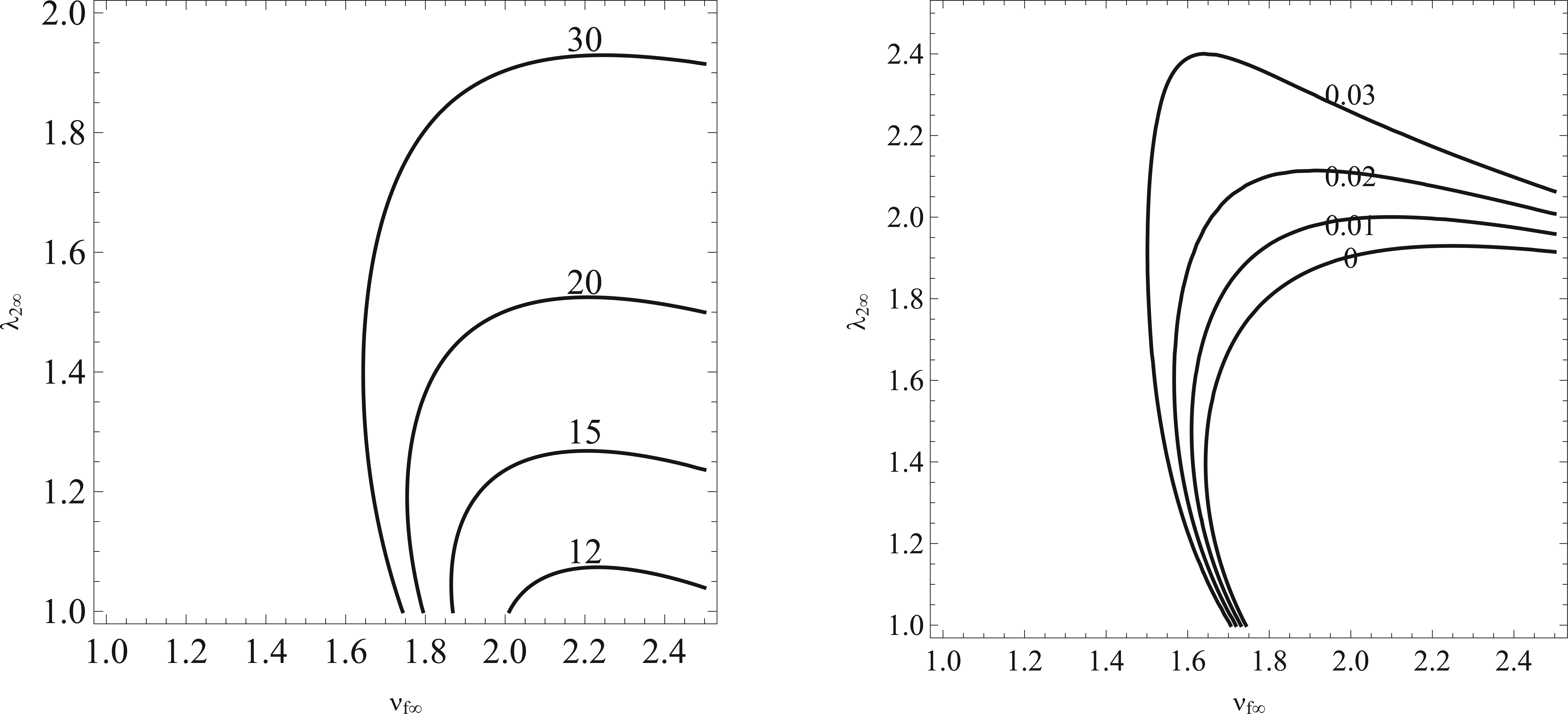
In Figure 4, we have shown how the solutions of the bifurcation condition (27) depend on $J_{m}$ and the quantity $v_{f 0} = b_{f} v_{f \infty}^{2} / 2$ . The figure on the left corresponds to $J_{m} = 30, 20, 15, 12$ with $v_{f 0} = 0$ , while the figure on the right corresponds to $v_{f 0} = 0, 0.01, 0.02, 0.03$ with $J_{m} = 30$ . We see that with $v_{f 0}$ fixed, increasing $J_{m}$ decreases $r_{cr}$ , whereas with $J_{m}$ fixed, increasing fluid inertia or the mean flow speed also reduces $r_{cr}$ . More importantly, we see from the form of the bifurcation condition (27) that even if localized bulging is not possible at all in the absence of a mean flow, it becomes possible when a large enough mean flow is present. However, for typical blood flows, $v_{f 0}$ is around $0.001$ and so its effect on the onset of bifurcation is negligible.

Figure 4.

Dependence of the solutions of (27) on $J_{m}$ (left) and $v_{f 0}$ (right).

To determine the localized bulging solutions when $r_{\infty}$ is not necessarily close to $r_{cr}$ , we evaluate the two integrals (31) and (32) at $Z = 0$ to obtain

W^{(0)} - z_{0} W_{2}^{(0)} = W^{(\infty)} - λ_{2 \infty} W_{2}^{(\infty)},

(41)

W_{2}^{(0)} - \frac{1}{2} r_{0}^{2} {P_{\infty} + \frac{1}{2} b_{f} v_{f \infty}^{2} (1 + \frac{λ_{1 \infty}^{4}}{r_{0}^{4}})} = W_{2}^{(\infty)} - \frac{1}{2} λ_{1 \infty}^{2} {P_{\infty} + b_{f} v_{f \infty}^{2}},

(42)

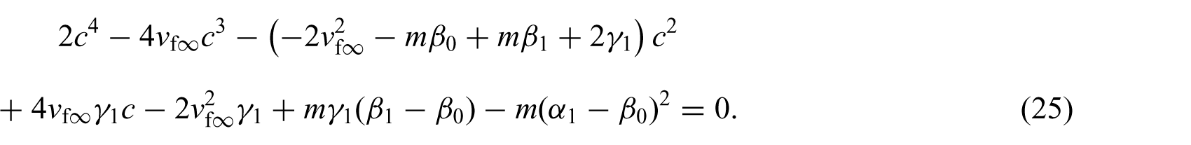
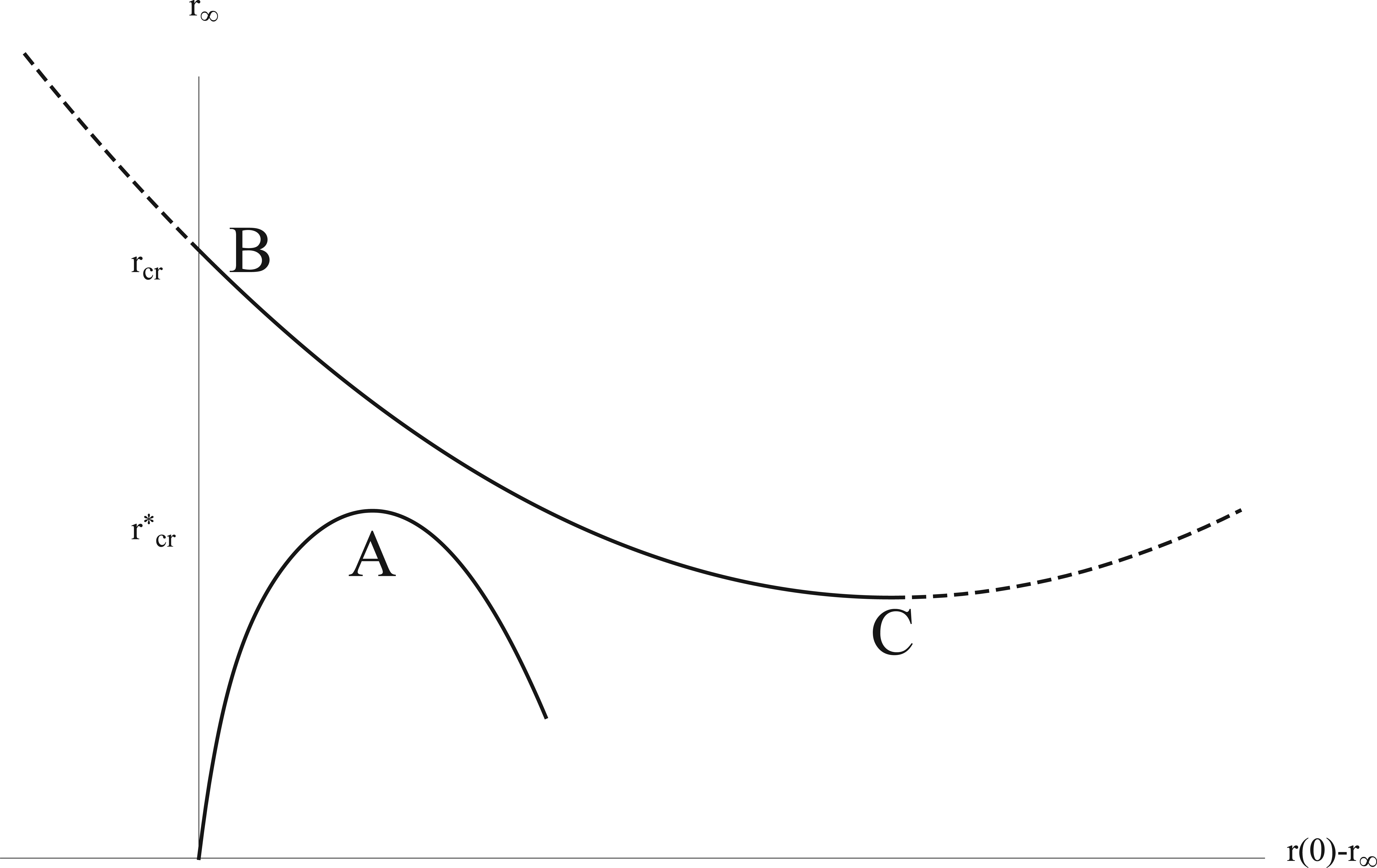
where $r_{0} = r (0), z_{0} = z' (0) = λ_{2} (0)$ . These two equations for the two unknowns $r_{0}$ and $z_{0}$ can be solved for each specified $r_{\infty}$ and $v_{f \infty}$ . The trivial solution $r_{0} = r_{\infty}$ and $z_{0} = λ_{2 \infty}$ is always a solution, but there also exist non-trivial solutions. A typical non-trivial solution is sketched in Figure 5 as the curve marked with points B and C, which has the following interpretation. Uniform inflation follows the vertical axis until the bifurcation point B is reached when a localized bulge will initiate. The post-critical localized bulging states correspond to the thin solid line, and we see that growth of the localized bulge is accompanied by a reduction in $r_{\infty}$ , the radius of the tube at infinity. The amplitude $r_{0} - r_{\infty}$ of the bulge grows as inflation continues until the turning point C is reached, after which the bulge no longer grows and instead it begins to propagate in the axial direction. The turning point C is determined by the property that $\partial r_{0} / \partial r_{\infty} \to \infty$ . With the use of (41) and (42), we find that this condition gives

W_{1}^{(0)} - r_{0} z_{0} P_{0} = 0,

(43)

where $P_{0}$ is given by the first equation in (30) with $r$ replaced by $r_{0}$ . This property together with the second equation in(15) implies that $r ″ (0) = 0$ . Thus, the solution corresponding to the turning point C is also a fixed point of the dynamical system (33). In the terminology of dynamical systems theory, when point C is approached from point B, a homoclinic orbit in the phase plane becomes a pair of heteroclinic orbits.

Figure 5.

A typical bifurcation diagram.

At each point along the thin solid line between B and C, the associated localized solution can be obtained by integrating (33) subject to the initial conditions $λ_{1} (0) = r_{0}, λ_{2} (0) = z_{0}, ϕ (0) = 0$ . As $C$ is approached, the solitary wave type solution becomes two kink wave type solutions stitched together at $Z = 0$ .

In Figure 5, we have also shown a typical curve (the thicker lower curve) showing the effects of imperfections such as localized wall thinning. In the presence of imperfections, the variation of $r_{\infty}$ again $r (0) - r_{\infty}$ would follow this curve which has a turning point. It was shown in Fu and Xie [6] that the reduction $r_{cr} - r_{cr}^{*}$ is proportional to the square root of the imperfection amplitude, and so the kind of subcritical bifurcation considered in the present paper is much more sensitive to imperfections than subcritical bifurcations into sinusoidal patterns which have been much studied in the context of shell structures.

5. Stability of the weakly nonlinear bulging solutions

An inspection of the dispersion relation (23) shows that in a small neighbourhood of $r_{\infty} = r_{cr}$ , the order of the wave speed of the slowest wave mode is determined by $c^{2} ~ ω ~ (r_{\infty} - r_{cr})$ if $v_{f}$ $= 0$ , and by $c ~ ω ~ (r_{\infty} - r_{cr})$ if $v_{f}$ $\neq 0$ . The former case has recently been examined by Il’ichev and Fu [8]. For the latter case, the appropriate spatial and time variables are $ξ$ and $τ$ , where $ξ$ is defined by the second equation in(38) and $τ$ is defined by $τ = ε^{3 / 2} t$ . We look for a perturbation solution of the form

r = r_{\infty} + ε {w_{1} (ξ, τ) + ε w_{2} (ξ, τ) + \dots}, r_{\infty} = r_{cr} - ε,

(44)

z = λ_{2 \infty} Z + \sqrt{ε} {u_{1} (ξ, τ) + ε u_{2} (ξ, τ) + \dots},

(45)

v_{f} = v_{f \infty} + ε v_{f 1} + \dots,

(46)

P = P_{\infty} + ε p_{1} (ξ, τ) + ε^{2} p_{2} (ξ, τ) + \dots,

(47)

where the relative orders of the perturbations have been deduced by considering dominant balance in the governing equations (15) and (16), and the order of perturbation of $r$ is deduced from the first equation in (38). For $P_{\infty}$ given by the fourth equation in (18) with $r_{\infty} = r_{cr} - ε$ , we have the Taylor expansion

P_{\infty} = \frac{W_{1} (r_{cr}, λ_{2 \infty})}{r_{cr} λ_{2 \infty}} + ε P_{1} + \dots .

(48)

On substituting (44)–(48) into (15) and (16), and equating the coefficients of like powers of $ε$ , we obtain a hierarchy of equations. For leading and second orders, we obtain $L y^{(1)} = 0$ and $L y^{(2)} = b$ , respectively, where $y^{(k)} = {(u_{k ″}, w_{k'}, p_{k'}, v_{f k}')}^{T}$ , $L$ is a $4 \times 4$ matrix that only depends on the uniform state (18), and the vector $b$ involves the leading order solution $y^{(1)}$ . It is then straightforward to show that det $L = 0$ recovers the bifurcation condition $ω (0, r_{cr}, v_{f}$ $) = 0$ , and that solvability of the second order problem yields an evolution equation of the form

\frac{\partial w_{1}}{\partial τ} - c_{0} \frac{\partial w_{1}}{\partial ξ} + c_{1} w_{1} \frac{\partial w_{1}}{\partial ξ} + c_{2} \frac{\partial^{3} w_{1}}{\partial ξ^{3}} = 0,

(49)

where $c_{0}, c_{1}$ , and $c_{2}$ are constants. Since (49) reduces to (37) when time independence is assumed, it must take the form

\frac{\partial \tilde{V}}{\partial τ} - c_{0} \frac{\partial \tilde{V}}{\partial ξ} + 2 c_{0} \tilde{V} \frac{\partial \tilde{V}}{\partial ξ} + c_{0} \frac{\partial^{3} \tilde{V}}{\partial ξ^{3}} = 0,

(50)

where

\tilde{V} = \frac{3 γ_{cr}}{2 {ω'}_{cr}} w_{1},

and the remaining constant $c_{0}$ can be found by looking for a travelling wave solution of the linearized form of (50) and then comparing the resulting dispersion relation with (23) . However, for our purpose this explicit expression is not needed. It suffices to observe that for $r_{\infty} < r_{cr}$ , the constant $c_{0}$ must necessarily be positive.

Equation (50) is recognized as a Korteweg–de Vries equation whose solution properties are well understood. Under the variable transformation $t^{*} = c_{0} τ, x = ξ + c_{0} τ, u = 2 \tilde{V}$ , this equation reduces to the standard form

\frac{\partial u}{\partial t^{*}} + u \frac{\partial u}{\partial x} + \frac{\partial^{3} u}{\partial x^{3}} = 0 .

(51)

The static solution (40) of (50) corresponds to the following travelling wave solution of (51):

u = 3 {sech}^{2} (\frac{1}{2} (x - t^{*})) .

It is known [35, 36] that this travelling wave solution is orbitally stable. It then follows that the static solution (40) of (50) is orbitally stable. This contrasts with the situation associated with $v_{f}$ $= 0$ , where the near-critical perturbations are governed by the Boussinesq equation and an unstable mode of perturbation always exists [8, 9].

6. Stability of the fully nonlinear bulging solutions

As remarked earlier, the fully nonlinear bulging solutions can be obtained by integrating the system of equations (33) whenever the amplitude diagram in Figure 5 becomes available. We denote such fully nonlinear bulging solutions by

r = \bar{r} (Z), z = \bar{z} (Z), P = \bar{P} (Z), v_{f} = {\bar{v}}_{f} (Z),

(52)

where $\bar{P} (Z)$ and ${\bar{v}}_{f} (Z)$ are obtained from (30) with $r$ replaced by $\bar{r} (Z)$ . To study their stability, we consider axisymmetric perturbations, and write

\begin{matrix} r (Z, t) = \bar{r} (Z) + Ψ (Z) e^{η t}, z (Z, t) = \bar{z} (Z) + Φ (Z) e^{η t}, \\ P (Z, t) = \bar{P} (Z) + Π (Z) e^{η t}, v_{f} (Z, t) = {\bar{v}}_{f} (Z) + V (Z) e^{η t}, \end{matrix}

where the mode functions $Ψ (Z), Φ (Z), Π (Z), V (Z)$ , and the growth rate $η$ are to be determined. On substituting these expressions into (15) and (16) and linearizing, we obtain

\begin{matrix} [\frac{1}{{\bar{λ}}_{2}} {\bar{W}}_{2} Φ' + \frac{\bar{z}'}{{\bar{λ}}_{2}^{3}} ({\bar{λ}}_{2} {\bar{W}}_{22} - {\bar{W}}_{2}) (\bar{r}' Ψ' + \bar{z}' Φ') + \frac{\bar{z}'}{{\bar{λ}}_{2}} {\bar{W}}_{12} Ψ] \\ - \bar{P} (\bar{r} Ψ' + Ψ \bar{r}') - \bar{r} \bar{r}' Π = η^{2} Φ, \end{matrix}

(53)

\begin{matrix} [\frac{1}{{\bar{λ}}_{2}} {\bar{W}}_{2} Ψ' + \frac{\bar{r}'}{{\bar{λ}}_{2}^{3}} ({\bar{λ}}_{2} {\bar{W}}_{22} - {\bar{W}}_{2}) (\bar{r}' Ψ' + \bar{z}' Φ') + \frac{\bar{r}'}{{\bar{λ}}_{2}} {\bar{W}}_{12} Ψ] \\ - \frac{1}{{\bar{λ}}_{2}} {\bar{W}}_{12} (\bar{r}' Ψ' + \bar{z}' Φ') - Ψ {\bar{W}}_{11} + \bar{P} (\bar{r} Φ' + Ψ \bar{z}') + \bar{r} \bar{z}' Π = η^{2} Ψ, \end{matrix}

(54)

η (\bar{z}' Ψ - \bar{r}' Φ) + {\bar{v}}_{f} Ψ' + V \bar{r}' + \frac{1}{2} \bar{r} V' + \frac{1}{2} Ψ \bar{v}'_{f} = 0,

(55)

b_{f} η (\bar{z'} V - \bar{v}'_{f} Φ) + b_{f} ({\bar{v}}_{f} V' + {\bar{v'}}_{f} V) + Π' = 0,

(56)

where a bar over $λ_{2}$ or $W$ signifies evaluation at the solution (52) . These equations can be written in the form

y' = M y,

(57)

where $y = {(Φ, Φ', Ψ, Ψ', Π, V)}^{T}$ and $M$ is a $6 \times 6$ matrix whose components are (numerically) known functions of $Z$ and $η$ . This system of equations are to be solved subject to the decay conditions $y \to 0$ as $Z \to \pm \infty$ .

Denoting by $M_{\infty}$ the limit of $M$ as $Z \to \pm \infty$ , and substituting a trial solution of the form $y = e^{\hat{k} Z} a$ into $y' = M_{\infty} y$ , we obtain the eigenvalue problem

(M_{\infty} - \hat{k} I) a = 0,

(58)

where $I$ is the $6 \times 6$ identity matrix. Non-trivial solutions correspond to $\det (M_{\infty} - \hat{k} I) = 0$ , which is simply the dispersion relation (23) under the substitutions

\hat{k} = i k \frac{λ_{2 \infty}}{r_{\infty}}, η = - i k \frac{c}{r_{\infty}} .

(59)

Recalling the properties of the dispersion relation (23) established in Section 3, we may immediately deduce that $\hat{k}$ can be imaginary only if $η$ is imaginary. This implies that if $η$ is confined to vary in the right half complex plane, $\hat{k}$ can never be imaginary. Since $k$ appears in (23) through $k^{2}$ , for each fixed $η$ , $- \hat{k}$ is a root whenever $\hat{k}$ is. Denote by ${\hat{k}}_{1}, {\hat{k}}_{2}, {\hat{k}}_{3}$ the three eigenvalues of (58) with negative real parts, and by $a_{1}, a_{2}, a_{3}$ the associated eigenvectors. Denote by $a_{1}^{-}, a_{2}^{-}, a_{3}^{-}$ the eigenvectors associated with the other three eigenvalues $- {\hat{k}}_{1}, - {\hat{k}}_{2}, - {\hat{k}}_{3}$ . There then exist solutions $y_{i} (Z)$ and $y_{i}^{-} (Z)$ of (57) such that

lim_{Z \to \infty} e^{- {\hat{k}}_{i} Z} y_{i} (Z) = a_{i}, lim_{Z \to - \infty} e^{{\hat{k}}_{i} Z} y_{i}^{-} (Z) = a_{i}^{-}, i = 1, 2, 3 .

Solutions of (57) that decay exponentially as $Z \to \infty$ and $Z \to - \infty$ , respectively, must be of the form

c_{1} y_{1} (Z) + c_{2} y_{2} (Z) + c_{3} y_{3} (Z) and c_{4} y_{1}^{-} (Z) + c_{5} y_{2}^{-} (Z) + c_{6} y_{3}^{-} (Z),

respectively, for some constants $c_{1}, c_{2}, \dots, c_{6}$ . The two solutions will match at any point, $Z = d$ say, to yield a localized eigen function, only if $η$ is such that

\det [y_{1} (d), y_{2} (d), y_{3} (d), y_{1}^{-} (d), y_{2}^{-} (d), y_{3}^{-} (d)] = 0 .

(60)

This is the most primitive way with which the eigenvalues of (57) can be determined, but because of the exponential behaviour of the solutions loss of independence of solutions occurs, which gives rise to numerical difficulties.

Alternatively, we may consider the exterior system [37, 38]

y^{\land'} = M^{\land} y^{\land},

(61)

and its adjoint system

x^{\land'} = - {(M^{\land})}^{T} x^{\land},

(62)

where the components of the vector function $y^{\land}$ come from all the $3 \times 3$ minors of the $6 \times 3$ matrix $(y_{1}, y_{2}, y_{3})$ , and the components of the $20 \times 20$ matrix $M^{\land}$ in terms of those of $M$ have previously been derived by Il’ichev and Fu [8].

It is known that if ${\hat{k}}_{1}, {\hat{k}}_{2}, \dots, {\hat{k}}_{6}$ are the eigenvalues of $M_{\infty}$ then the matrix $M_{\infty}^{\land}$ has eigenvalues

{\hat{k}}_{i} (η) + {\hat{k}}_{j} (η) + {\hat{k}}_{l} (η), 1 \leq i < j < l \leq 6 .

Thus, the asymptotic matrix $M_{\infty}^{\land}$ has simple left-most eigenvalue $k^{\land} (η) = {\hat{k}}_{1} (η) + {\hat{k}}_{2} (η) + {\hat{k}}_{3} (η)$ for $η$ in the right half-plane. We denote by $r^{\land} (η)$ the right eigenvector of $M_{\infty}^{\land}$ associated with the eigenvalue $k^{\land} (η)$ , and by $1^{\land} (η)$ the corresponding left eigenvector. It is easily seen that $1^{\land} (η)$ is then the right eigenvector of $- {(M^{\land})}^{T}$ in (62) associated with the eigenvalue $- k^{\land} (η)$ . Solving (61) and (62) subject to the initial conditions

y^{\land} (Q) = r^{\land} (η), x^{\land} (- Q) = 1^{\land} (η),

respectively, where $Q$ is a sufficiently large positive number, we obtain two solutions $y^{\land} (η, Z)$ and $x^{\land} (η, Z)$ . It follows from (61) and (62) that the dot product of these two solutions is independent of $Z$ .

The Evans function is defined by

D (η) = x^{\land} (η, Z) \cdot y^{\land} (η, Z),

(63)

and it can be shown that the matching condition (60) is equivalent to $D (η) = 0$ . Thus, eigenvalues associated with unstable localized eigen modes are determined by $D (η) = 0$ .

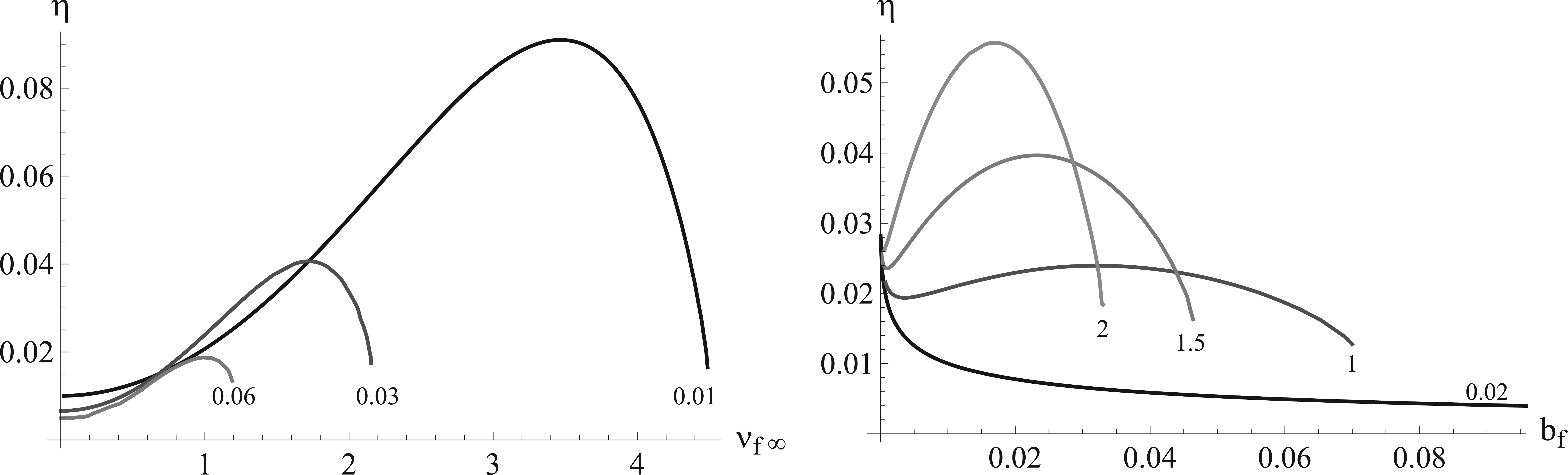
By adapting theMathematica code used in [8], we find that for each fixed value of $b_{f}$ there exist two unstable eigenvalues for $v_{f \infty}$ less than a threshold value. At this threshold value, the two unstable eigenvalues coalesce and no unstable eigenvalues exist for $v_{f \infty}$ greater than this threshold value. Likewise, for each fixed value of $v_{f \infty}$ there exist two unstable eigenvalues for $b_{f}$ less than a threshold value. At such a threshold value, the two unstable eigenvalues coalesce and no unstable eigenvalues exist for $b_{f}$ greater than this threshold value. Figure 6 illustrates these facts for the case when $r_{\infty} = 1.41, z_{\infty} = 1.2$ , and the material is modeled by the Gent model with $J_{m} = 30$ . For each value of $b_{f}$ or $v_{f \infty}$ considered, we have not shown the lower branch of the growth rate curve because it is always zigzagged, and so we believe that our numerical results may not be reliable. One possible explanation for the zigzag behaviour is that at each lower branch the growth rate is very small; it is typically of order $0.001$ , and so the $η^{2}$ in (53) – (56) is of order $10^{- 6}$ . Our numerical scheme is expected to become invalid in the limit $η \to 0$ because in this limit two pairs of the eigenvalues of $M_{\infty}$ determined by (58) are zero, and correspondingly, the left-most eigenvalue $k^{\land} (η)$ of $M_{\infty}^{\land}$ becomes a repeated eigenvalue with multiplicity of 6. We will examine the lower branch behaviour more thoroughly in a separate study. For our current purpose, it suffices to confirm that no unstable modes can exist when the mean flow speed becomes large enough. For a typical rubber tube containing water with a mean flow speed of $40$ cm/s (which is the typical blood flow speed in arteries), $b_{f}$ and $v_{f \infty}$ are approximately equal to $3.47$ and $0.02$ , respectively. Figure 6 shows that when $v_{f}$ $= 0.02$ , the localized bulging solution is completely stabilized when $b_{f}$ reaches the threshold value of $0.14$ , much less than $3.47$ .

Figure 6.

Left: Variation of the growth rate with respect to $v_{f \infty}$ for three representative values of $b_{f}$ , $0.01, 0.03,$ and $0.06$ . Right: Variation of the growth rate with respect to $b_{f}$ for four representative values of $v_{f \infty}$ , $0.02, 1, 1.5,$ and $2$ . Each curve is joined by a lower branch at the turning point, which is not shown because of unreliable numerical results.

7. Conclusion

Our present study is aimed at providing the last building block for the framework of a mathematical theory concerning the initial formation of aneurysms in human arteries. Under this theory, the initial formation of aneurysms is interpreted as a bifurcation phenomenon, just as localized bulging in inflated tubular rubber balloons. Since we assume that it is the formation and stable presence of a localized bulge that triggers the subsequent remodelling process, the stability of such a localized bulge is essential if our theory is to have any relevance. It is shown that although a mean flow (such as the natural blood flow) may only have a negligible effect on the critical pressure, it does change the stability properties of localized bulges qualitatively. In the absence of a mean flow, evolution of near-critical modes obeys the Boussinesq equation which has a single unstable mode, but when a mean flow is present, the evolution equation becomes the Korteweg–de Vries equation whose travelling wave solutions are always stable. The Evans function method that we used to check stability of the fully nonlinear bulging solutions is a very effective tool to establish spectral instability (exponential linear growth), but it cannot establish stability conclusively in the present case. In fact, even if the static bulging solution is orbitally stable, it can still travel under perturbations although this becomes impossible as soon as the translational invariance is broken (which occurs, for instance, when the tube is subject to localized wall thinning). We are currently looking for alternative ways to prove stability in the presence of localized wall weakening and, in the meantime, experimental verification is also being carried out by an experimental mechanics group.

Before our theory can be used to guide any drug development (assuming that drugs can modify the constitutive behaviour of arteries), the greatest challenge is to verify that localized bulging can indeed take place as a bifurcation in some live arteries under realistic physiological conditions. Ideally, we would like to see that when the artery has no localized weakening, the bifurcation pressure is extremely high, but as soon as localized wall weakening is introduced the actual bifurcation pressure (corresponding to point A in Figure 5) will come down to around 120 mmHg. We expect this scenario because for human arteries pressure is believed to be an exponential function of the principal stretches. We do not, however, expect localized bulging to be theoretically possible for all human arteries because of their huge varieties. The calculations conducted in [7] show that some arterial models predict bifurcation almost too easily whereas some other models used predict no bifurcation. Since the prediction of our theory is only as good as the arterial models employed, application of our theory would require more accurate constitutive modelling of human arteries.

We also observe that our one-dimensional averaged model for the fluid flow is expected to fail when the size of the localized bulge becomes significant. We are currently planning a fully numerical simulation of the fluid–solid interaction problem by considering the fluid flow to be fully three dimensional but still assuming axi-symmetry. We are thus looking for a fluid–solid coupled and fully nonlinear solution that bifurcates from the uniform state (18). The fully nonlinear bifurcation solution determined in Section 4 is expected to provide an excellent initial guess in any iteration scheme. Other effects that we wish to address in future include bending stiffness of the arterial wall, and the viscous, viscoelastic, and pulsatile nature of the blood flow.

Footnotes

Funding

This work was supported by a Joint Project grant awarded by the Royal Society and Russian Foundation for Basic Science Research, and by the National Science Foundation of China (grant no. 11372212).

References

McGloughlin

(ed). Biomechanics and Mechanobiology of Aneurysms. New York: Springer, 2011.

Lasheras

. The biomechanics of arterial aneurysm. Annu Rev Fluid Mech 2007; 39: 293–319.

Humphrey

. Cardiovascular Solid Mechanics. New York: Springer, 2002.

Watton

Hill

Heil

. A mathematical model for the growth of the abdominal aortic aneurysm. Biomechan Model Mechanobiol 2004; 3: 98–113.

Pearce

Liu

. Post-bifurcation analysis of a thin-walled hyperelastic tube under inflation. Int J Non-Lin Mech 2008; 43: 697–706.

Xie

. Effects of imperfections on localized bulging in inflated membrane tubes. Phil Trans R Soc A 2012; 370: 1896–1911.

Rogerson

Zhang

. Initiation of aneurysms as a mechanical bifurcation phenomenon. Int J Non-Lin Mech 2012; 47: 179–184.

Il’ichev

. Stability of aneurysm solutions in a fluid-filled elastic membrane tube. Acta Mechanica Sinica 2012; 28: 1209–1218.

Pearce

. Characterisation and stability of localised bulging/necking in inflated membrane tubes. IMA J Appl Math 2010; 75: 581–602.

10.

Kyriakides

Chang

Y-C

. The initiation and propagation of a localized instability in an inflated elastic tube. Int J Solid Struct 1991; 27: 1085–1111.

11.

Pamplona

Goncalves

Lopes

SRX

. Finite deformations of cylindrical membrane under internal pressure. Int J Mech Sci 2006; 48: 683–696.

12.

Shi

Moita

. The post-critical analysis of axisymmetric hyper-elastic membranes by the finite element method. Comput Methods Appl Mech Engrg 1996; 135: 265–281.

13.

Chater

Hutchinson

. On the propagation of bulges and buckles. ASME J Appl Mech 1984; 51: 269–277.

14.

Yin

W-L

. Non-uniform inflation of a cylindrical elastic membrane and direct determination of the strain energy function. J Elast 1977; 7: 265–282.

15.

Kirchgässner

. Wave solutions of reversible systems and applications. J Diff Eqns 1982; 45: 113–127.

16.

Laleg

T-M

Creṕeau

Sorine

. Separation of arterial pressure into a nonlinear superposition of solitary waves and a windkessel flow. Biom Sign Proc Control 2007; 2: 163–170.

17.

Noubissé

Kraenkel

Woafo

. Disturbance and repair of solitary waves in blood vessels with aneurysm. Comm Nonlinear Sci Num Simu 2009; 14: 51–60.

18.

Yomosa

. Solitary waves in large blood vessels. J Phys Soc Jpn 1987; 56: 506–520.

19.

Demiray

Dost

. Axial and transverse solitary waves in prestressed elastic tubes. ARI 1998; 50: 1065–1079.

20.

Epstein

Johnston

. On the exact speed and amplitude of solitary waves in fluid-filled elastic tubes. Proc R Soc Lond A 2001; 457: 1195–1213.

21.

Il’ichev

. Solitary waves in fluid-filled elastic tubes: Existence, persistence, and the role of axial displacement. IMA J Appl Math 2010; 75: 257–268.

22.

Haughton

Ogden

. Bifurcation of inflated circular cylinders of elastic material under axial loading. I Membrane theory for thin-walled tubes. J Mech Phys Solids 1979; 27: 179–212.

23.

Gent

. A new constitutive relation for rubber. Rubber Chem Technol 1996; 69: 59–61.

24.

Horgan

Saccomandi

. A description of arterial wall mechanics using limiting chain extensibility constitutive models. Biomechan Model Mechanobiol 2003; 1: 251–266.

25.

Holzapfel

Ogden

. Constitutive modelling of arteries. Proc R Soc A 2010; 466: 1551–1597.

26.

Demiray

. Solitary waves in initially stressed thin elastic tubes. Int J Non-Lin Mech 1996; 32: 1165–1176.

27.

Chen

Y-C

. Stability and bifurcation of finite deformations of elastic cylindrical membranes—Part I: Stability analysis. Int J Sol Struct 1997; 34: 1735–1749.

28.

Callaghan

Geddes

Babbs

. Relationship between pulse-wave velocity and arterial elasticity. Med Biol Eng Comput 1986; 24: 248–254.

29.

Blacher

Asmar

Djane

. Aortic pulse wave velocity as a marker of cardiovascular risk in hypertensive patients. Hypertension 1999; 33: 1111–1117.

30.

Bronshtein

Semendyayev

. Handbook of Mathematics. Berlin: Springer, 1997.

31.

Wolfram

. Mathematica: A System for Doing Mathematics by Computer. 2nd edition.Redwood City, CA: Addison-Wesley, 1991.

32.

Mielke

. Hamiltonian and Lagrangian Flows on Center Manifolds, with Applications to Elliptic Variational Problems (Lecture Notes in Mathematics, Vol. 1489). Berlin: Springer, 1991.

33.

Iooss

Kirchgässner

. Water waves for a small surface tension: An approach via normal form. Proc R Soc Edin A 1992; 122: 267–299.

34.

Iooss

Adelmeyer

. Topics in Bifurcation Theory and Applications. Singapore: World Scientific, 1999.

35.

Benjamin

. The stability of solitary waves. Proc R Soc A 1972; 238: 153–183.

36.

Bona

. On the stability of solitary waves. Proc R Soc A 1975; 344: 363–374.

37.

Alexander

Sachs

. Linear instability of solitary waves of a Boussinesq-type equation: A computer assisted computation. Nonlin World 1995; 2: 471–507.

38.

Pego

Weinstein

. Eigenvalues, and instability of solitary waves. Phil Trans R Soc Lond A 1992; 340: 47–94.