In this paper the linearized equations of motion in multibody dynamics are derived. Explicit expressions for the coefficient matrices are presented and given their physical interpretations. The equations of motion are presented in terms of the mechanical stiffness, its adjoint and the associated differential operators. It is demonstrated how the adjoint matrix may be used to find solutions to the associated algebraic eigenvalue problem. The case of multiple roots of the characteristic equation will result in a generalized eigenvalue problem involving the notion of a Jordan chain. Qualitative properties of the spectrum are derived without explicitly solving the characteristic equation. Finally, the mechanical admittance and its spectral representations are discussed.
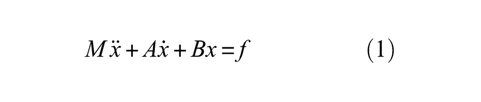
The equations of motion in multibody dynamics constitute a system of ordinary differential equations of the second order. Typically they are non-linear and a detailed analysis of their solutions is usually very complicated. In many cases only qualitative aspects of their properties are accessible and for quantitative information one has to rely on numerical methods. If equilibrium configurations are present for the multibody system, solutions representing its motion in the vicinity of the equilibrium configuration may appear. The existence of these so-called mechanical vibrations is determined by the stability properties of the system at the equilibrium configuration. The analysis of mechanical vibrations is based on the linearized equations of motion. These equations are linear in the configuration coordinates, and their first- and second-order time derivatives. They are usually written in the standard format
where the configuration coordinate represents the deviation of the system from the equilibrium configuration, is the mass matrix at the equilibrium configuration and are matrices representing dissipative and stiffness properties, as well as certain aspects of inertial and external forces that may appear as a consequence of, for instance, the choice of configuration coordinates. The column matrix , on the right-hand side of the equation, represents the specific time-dependent part of the external force on the system. Equation (1) is one of the classical equations in structural dynamics modelling the vibrations of structures with a finite number of degrees of freedom. Its history goes back to the early days of rational mechanics and the pioneering work by Euler and Lagrange. The status of the subject, as of the late 19th century, is accounted for by Lord Rayleigh [1]. Theories and methods presented in this classical and often-cited work are still of significance in the field. More recent numerical methods, such as the finite element method, have renewed the interest in the equation concerning both formal mathematical aspects as well as numerical techniques (see Hughes [2]).
The formulation of the linear ordinary differential equation (1) requires a calculation of the coefficient matrices , and . Starting from the basic equations of motion in multibody dynamics, one identifies the equilibrium solutions and then performs a formal linearization of the equations at an equilibrium configuration. The mathematical character of the coefficient matrices will then follow from physical properties of the system and from the method underlying the formulation of the basic equations. If the derivation of the basic equations is obtained by using the method of Lagrange, the mass matrix will always be symmetric (see, for instance, Géradin and Rixen [3]). For many multibody systems this will be the case for the matrices and as well. However, there are important systems where this is not so.
In this paper we consider a multibody system consisting of rigid and visco-elastic parts connected by ideal joints. Starting from the basic equations of motion, as presented by Lidström [4], linearized equations at an equilibrium configuration are derived. The coefficient matrices and are then identified and characterized in terms of their general mathematical properties and physical interpretations.
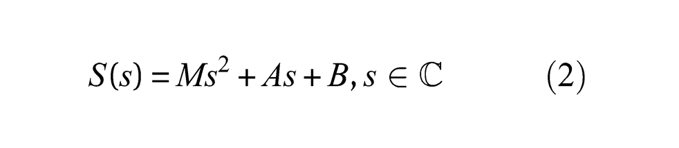
The differential equation (1) is closely related to the matrix polynomial
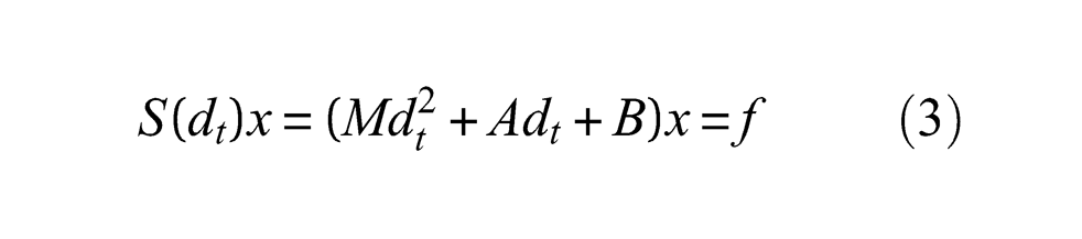
called the dynamic stiffness of the multibody system at the equilibrium configuration. Equation (1) may then be written
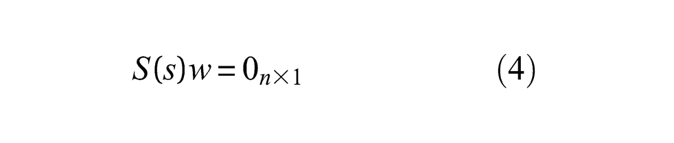
where is the ordinary differential operator with respect to time. It is well known that the associated eigenvalue problem: find and such that
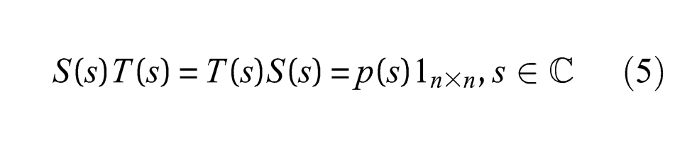
plays an important role for the solution of Equation (3). The existence of a non-trivial solution to the eigenvalue problem requires that satisfies the characteristic equation, where is the characteristic polynomial associated with the dynamic stiffness. The roots of the characteristic equation define the spectrum of the differential operator (3). The adjoint associated with the dynamic stiffness is the unique matrix satisfying
In this paper we make a systematic use of the adjoint matrix and its related adjoint differential operator to construct solutions to (3). This is a different approach than usually taken in books on ordinary differential equations such as, for instance, Birkhoff and Rota [5] and Arnold [6]. The standard procedure there is to transform Equation (3) into a system of first-order differential equation, the so-called state space formulation. This is, from the mathematical point of view, a rational and unifying approach. The advantage of the method used here is that it retains the original differential equation (3) with its close connection to the basic principles of mechanics. We suspect that the approach of using the adjoint, if not entirely new, is not too well known in the engineering community.
The objective of this paper is to derive the linearized equations of motion in multibody dynamics, to analyse their properties and characterize their solutions in the cases where the coefficient matrices and represent properties of the mechanical system that are not too special. The classical solution procedure of Equation (3) is to try to find a linear coordinate transformation that will uncouple the differential equations (see Foss [7] and Caughey [8]). This procedure works if the coefficient matrices and are symmetric and if, in addition, (see Caughey and O’Kelly [9]). A situation of this kind is, for instance, at hand in the case of so-called proportional damping. If or are not symmetric the situation is more complicated. Results covering some of these more general cases are found in Lancaster [10], a work that will be frequently referred to in this paper.
There are many textbooks on mechanical vibrations. One good example is the previously mentioned book by Géradin and Rixen [3], where some attention is given to the derivation of the linearized equation. Concerning the properties of the solutions to the equations, the literature is abundant and a full review will not be undertaken here. Most papers deal with special applications often resulting in equations where the matrices and are symmetric and they use solution methods involving changes of coordinates in order to obtain uncoupled or nearly uncoupled equations. The presentation of more general methods, in order to find solutions to the equations, will be one of the main themes of this paper.
The paper is organized as follows. In Section 2 the basic notations and definitions used throughout the paper are reviewed. In Section 3 the multibody system and its configuration coordinates are introduced along with the equations of motion. Section 4 specifies the interaction between parts and constitutive assumptions for rigid and visco-elastic parts. Section 5 defines the equilibrium configuration and derives the linearized equation of motion. The coefficient matrices are calculated and given their appropriate physical interpretations. A linearized version of the power theorem is derived. In Section 6 general properties of the linearized equation are discussed involving, among other things, the existence and uniqueness of solutions. Two elementary examples, illustrating the theory, are presented. In Section 7 free vibrations are analysed using the adjoint differential operator. This will result in the so-called characteristic differential equation. Solutions of this equation, which are well known in the mathematical literature, are accounted for as exponential-polynomials. In Section 8 the important case of simple roots to the characteristic equation is discussed. This will, for instance, result in the eigenvalue problem defined in (4) above. It is demonstrated how the adjoint matrix may be used to find solutions to this eigenvalue problem. In Section 9 the case of multiple roots is discussed. This will result in a generalized eigenvalue problem involving the notion of a Jordan chain. The case of a so-called simple dynamic stiffness matrix is given special attention. In Section 10 the dynamic flexibility is defined as the inverse of the dynamic stiffness. It is evaluated in the case of a simple dynamic stiffness and related to modal properties. In the general case a basic formula for the flexibility is derived, but without an explicit relation to its modal properties. In Section 11 qualitative properties of the spectrum are discussed. This is done without explicitly solving the characteristic equation. The results are illustrated in a simple example. In the final section, Section 12, forced vibrations are characterized using the dynamic flexibility.
To facilitate the reading of this paper some of the mathematical notation, definitions and results used in the main text are filed in an Appendix.
2. Notations
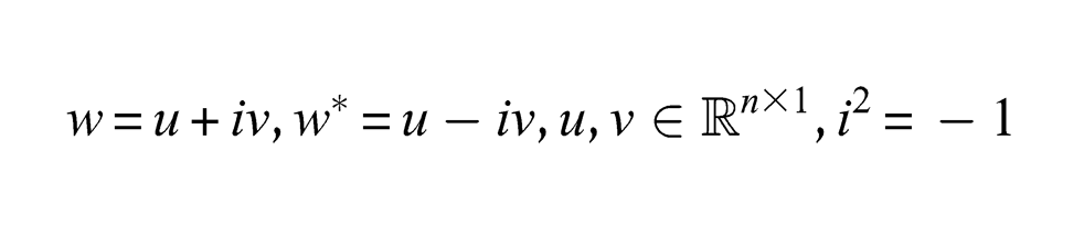
In this paper denotes the set of natural numbers (not including ), denotes the set of real numbers, denotes the set of positive real numbers and the set of complex numbers. If then denotes its complex conjugate. Detailed information on matrix notation and definitions are collected in the Appendix.
Let denote a three-dimensional Euclidean point space with the corresponding translation vector space , that is, . Points in are denoted by and vectors in by . The scalar product of two vectors is denoted . The norm of a vector a is defined by . The boundary of a set is denoted . The space of all second-order tensors A on , that is, linear mappings , is denoted . We write for the unit tensor in and for the transpose of . The space of all symmetric tensors is denoted by and the space of skew-symmetric tensor is denoted . The scalar product, , of two tensors is defined by and the corresponding norm .
3. Equations of motion in multibody dynamics
This introductory section follows closely that of Lidström [4]. For more information on details and motivations for the present approach the reader is referred to that paper.
Consider a multibody consisting of rigid or elastic parts: . Let the regular region in denote the present (spatial) placement of , at time t. The function representing the transplacement of the part from its reference placement to its present placement is given by the mapping , where
is the present place (at time ) of the material point with its referential place denoted by . We assume that it is possible to introduce configuration coordinates
where is an open set, so that the set of possible placements (configurations) of the parts of the multibody may (locally) be represented by the mappings
where is assumed to be a twice continuously differentiable mapping in all its arguments . The deformation gradient and the Green–St. Venant strain tensor are defined by and , respectively.
The motion of the multibody is given by a function and a mapping
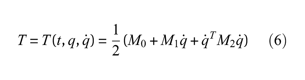
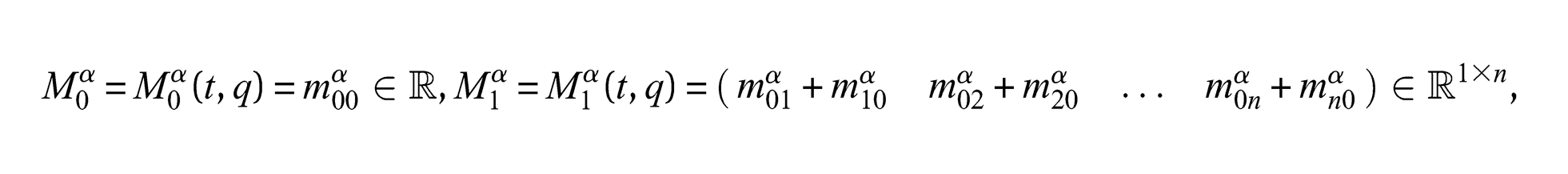
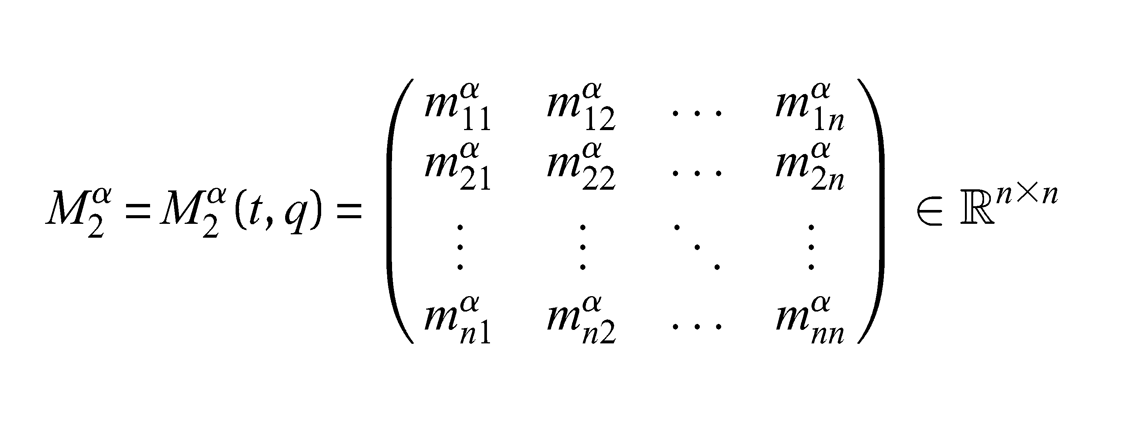
Let denote the mass density of part in its reference placement. The kinetic energy for the multibody may be written
where , , and
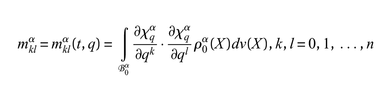
where the matrix elements are defined by
The matrix is symmetric and positive semi-definite. We will here assume that the system of configuration coordinates is regular, which implies that is positive definite (see Lidström [4]).
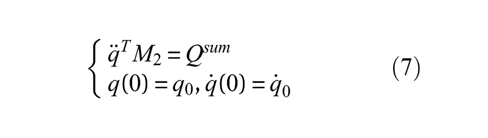
The equations of motion for the multibody may now, according to Lidström [4], be written
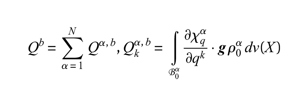
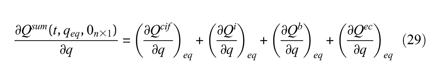
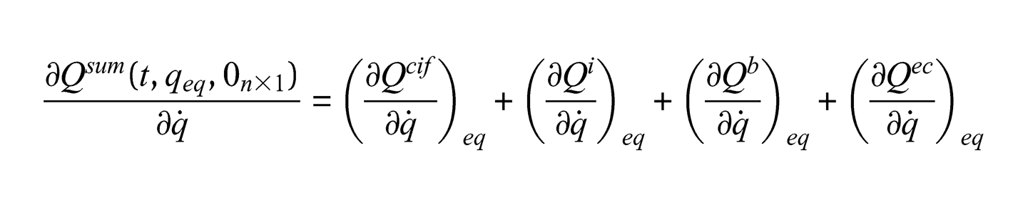
where the sum of the generalized forces represents the sum of external as well as internal forces acting on the multibody system. It is convenient to express the force sum according to
where , the complementary inertia force, represents inertial forces such as centrifugal and Coriolis forces, is the internal force, is the contact force and is the body force due to gravity. The complementary inertia force is defined by (see the Appendix in Lidström [4] for a definition of derivatives of matrix valued functions)
and the internal force by
where
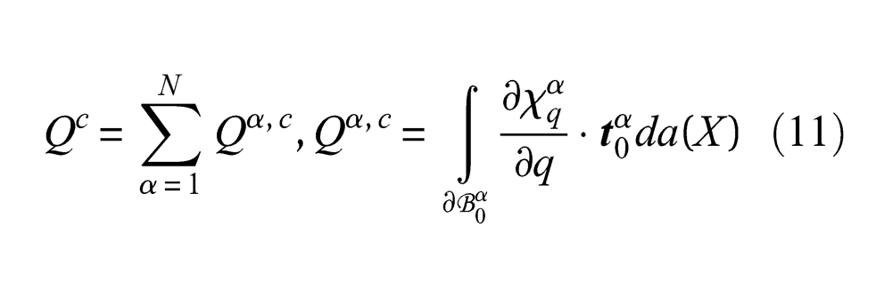
is the internal force corresponding to part . In Equation (10) is the Green–St. Venant strain tensor defined above and denotes the second Piola–Kirchhoff stress tensor. The generalized contact force is defined by
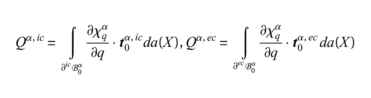
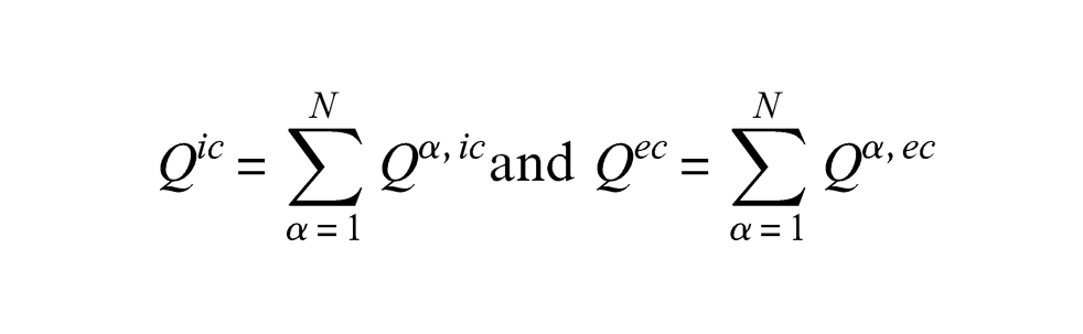
where is the traction vector on the boundary surface of part . We may employ the decomposition , where is the internal contact force, that is, the contact force acting on part from all other parts of and is the external contact force on part , from the exterior of . This force is assumed to be prescribed. We may write
where is the prescribed traction vector acting on from the exterior of and represents the boundary of in contact with the exterior of , while is the contact surfaces between and all other parts of and is the corresponding traction vector. With
it follows that . One may write
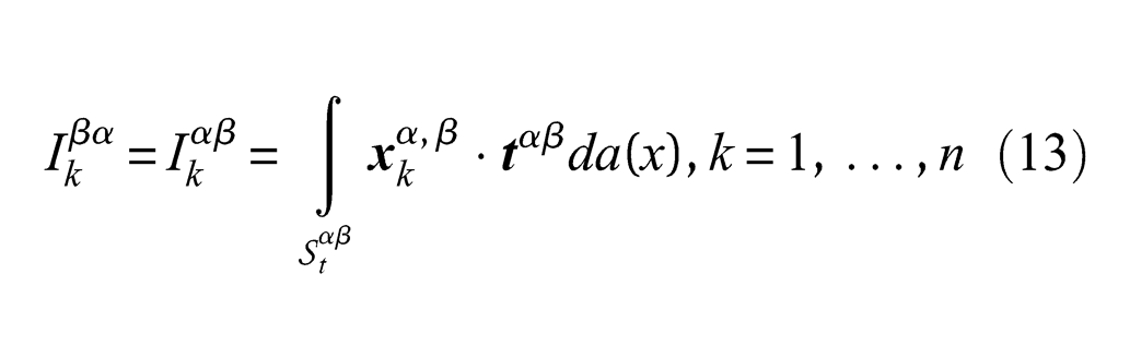
where the interaction, between parts and , is given by
where is the contact surface between parts and in their present placements, and and is the traction vector acting on from in their present placement (see Lidström [4]).
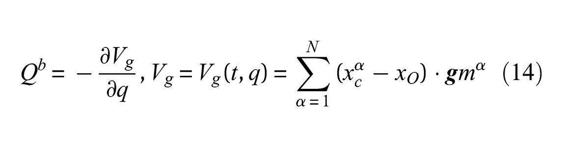
The generalized body force is here assumed to be due to gravity. Then
where is the (constant) acceleration of gravity. Thus
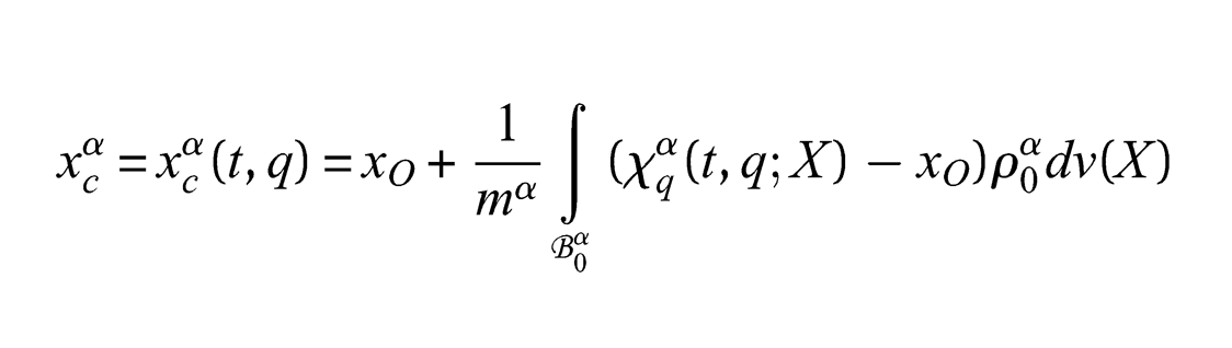
where is the mass of part and
is the present place of the centre of mass of part . The point is assumed to have a fixed place in Euclidean space.
4. Constitutive assumptions and interactions between parts
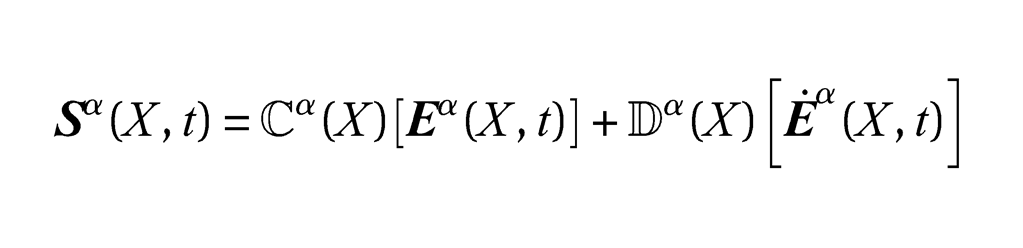
The constitutive equation for a visco-elastic part is given by
where and are symmetric, positive semi-definite linear mappings, that is, and . Then
Proposition 4.1
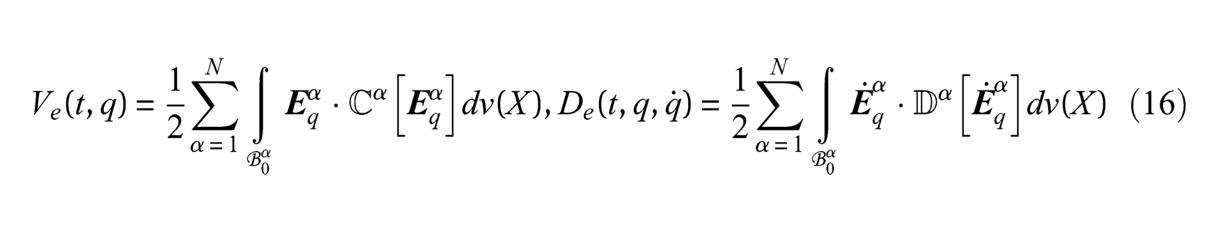
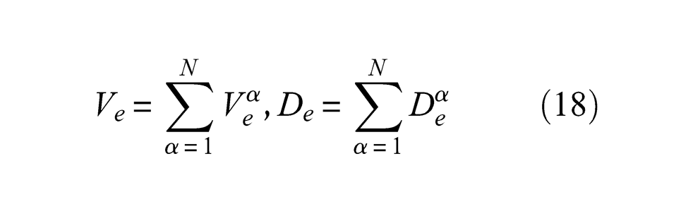
where
are the elastic energy and the Rayleigh dissipation function of the multibody , respectively.
Proof: We note that
and consequently . Then, considering part ,
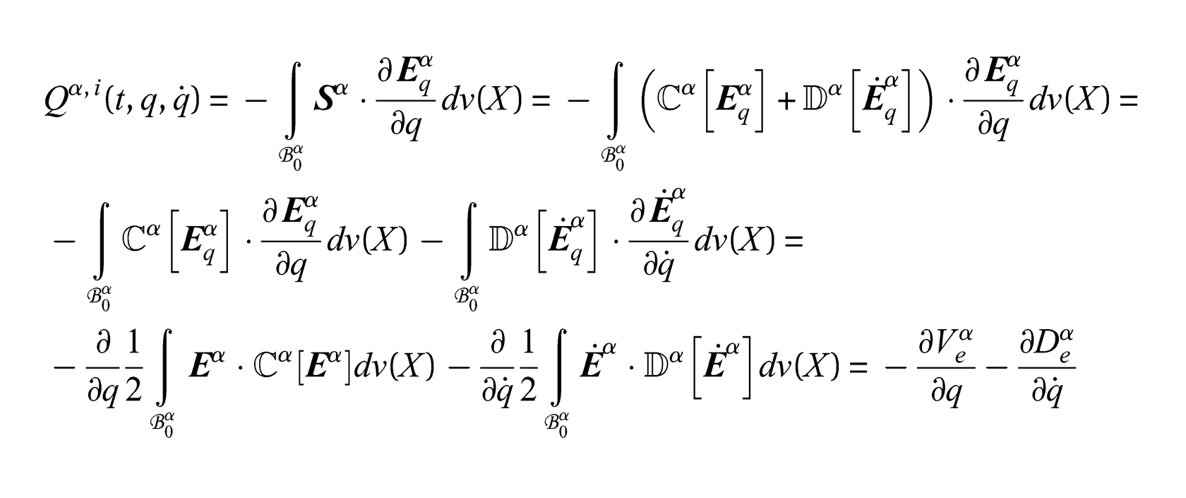
where and are defined in (16). Consequently, the generalized internal force for the multibody may then be written
where
This proves the proposition. □
Note that if part is rigid then , and, consequently, in this case, , which means that rigid parts do not contribute to the generalized internal force of the multibody.
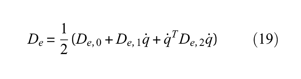
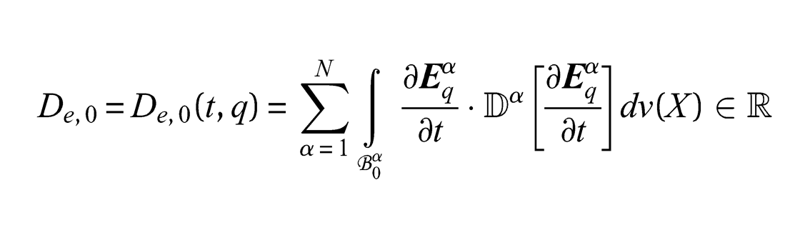
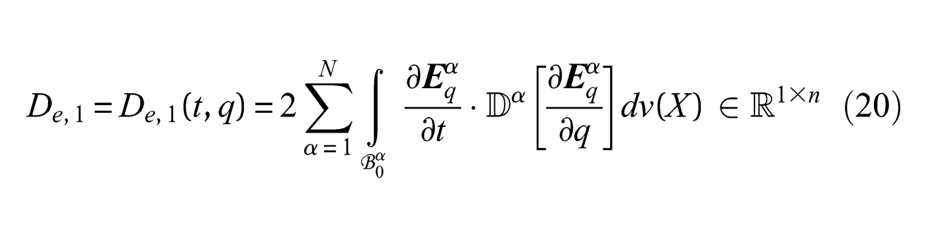
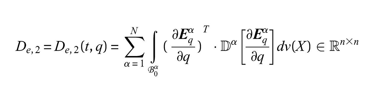
Proposition 4.2 The Rayleigh dissipation function
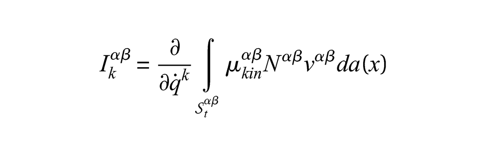
where
and is a symmetric, positive semi-definite matrix. Consult the Appendix A.1 for a definition of the integrands appearing in (20).
Proof: A demonstration is obtained by inserting (17) into (16)2. □
Interactions between parts are mediated by the internal contact forces and summarized in according to Equation (12). Characteristic of multibody systems is the presence of joints that impose constraints on the relative motion between parts of the system. Many joints, in practical applications, may be modelled in terms of so-called simple joints; examples are the cylindrical, prismatic, screw, revolute, spherical and planar joints. In this paper we assume that the q-coordinate system is compatible with the constraints, that is, the constraint conditions are identically satisfied for all . Then, according to Lidström [4]:
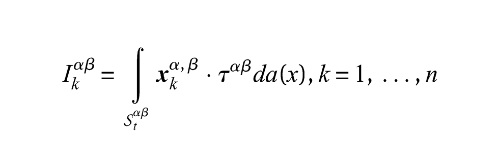
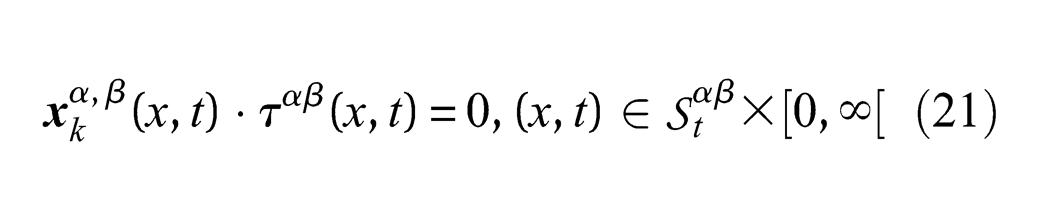
where denotes the tangential composant of the contact force , that is, where denotes the orientation of the contact surface . We now assume that
The interaction is then said to be ideal and it follows that and according to (12) we then have and consequently
Ideal joints may be equipped with visco-elastic torsion bushing elements that will add to the interactions of the multibody (see Lidström [11]). The interaction may also be mediated by a torque obtained from an electric motor acting between parts and . These possibilities will, however, not be considered in this paper.
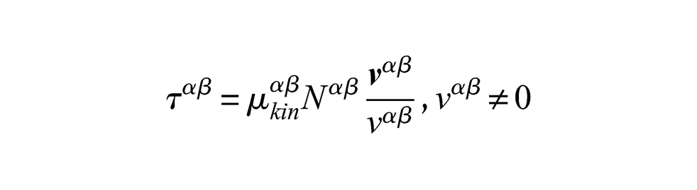
Remark 4.1: The assumption in (21) rules out the influence of Coulomb friction at contact surfaces. The incorporation of Coulomb friction would require an expression for of the form
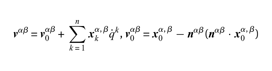
where is the coefficient of kinematic friction at the contact surface between parts and , is the normal component of the contact traction, that is, , is the relative tangential material velocity at the contact surface, that is, and . If the q-coordinate system is compatible with the constraints then (see Lidström [4])
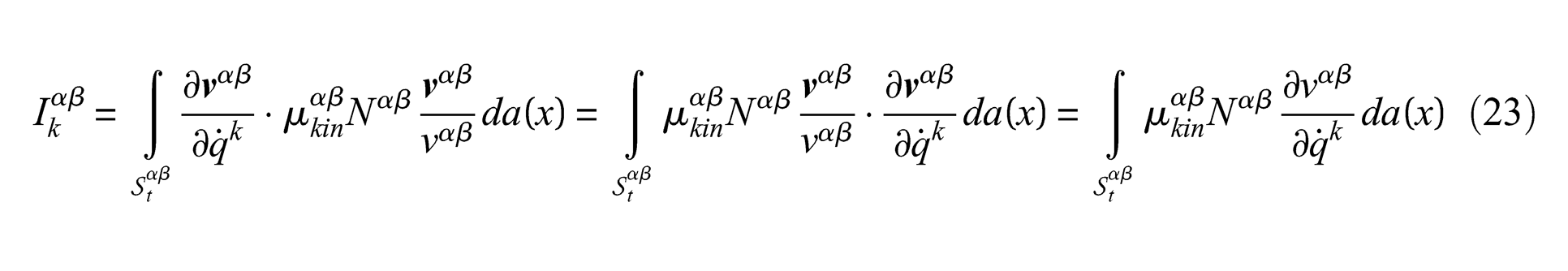
Thus and then
where we have used the identity . If we introduce the (heuristic) assumption that and do not depend on then (see Géradin and Rixen [3], p. 24–25)
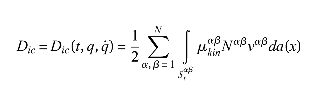
and we may write where
is the Rayleigh dissipation function corresponding to the internal contact forces due to Coulomb friction. The assumption that , in general, does not depend on is most certainly not correct. Furthermore, may, in more advanced friction models, depend on . A calculation of requires, according to (23), a calculation of the normal force . In order to obtain this one has to introduce a q - coordinate system, which is not compatible with the constraints (see Lidström [12]). We do not consider this much more complicated situation in the present paper.■
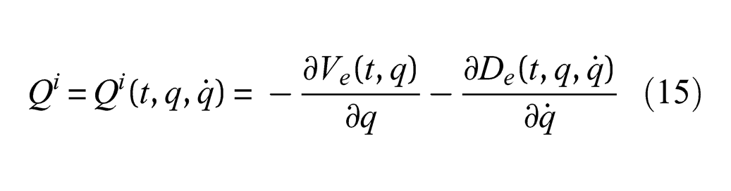
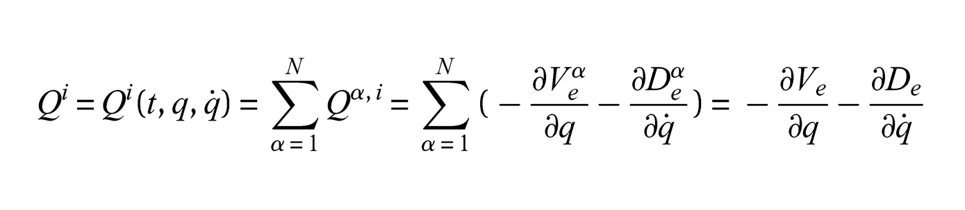
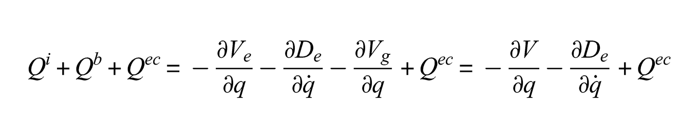
The sum of the generalized forces (except ) may, if and are given by (14) and (15), be written
where
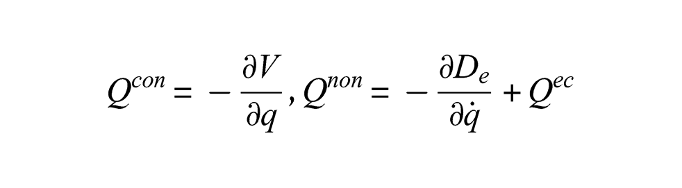
is the potential energy of the multibody. We have the following division into conservative and non-conservative forces:
where
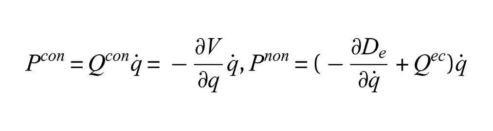
The power expended by these forces is given by
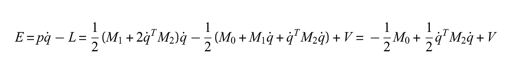
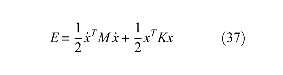
The mechanical energy, E, of the multibody is defined by
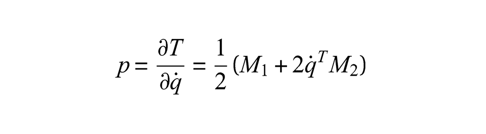
where is the Lagrangian, and is the so-called generalized momentum.
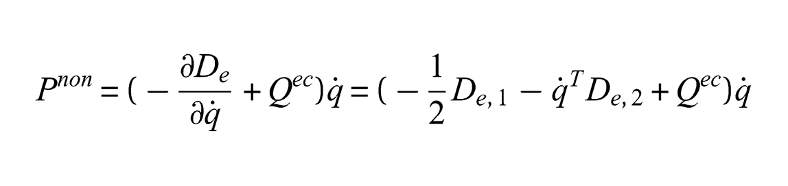
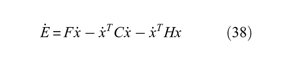
Proposition 4.3 The power theorem for the multibody reads
where in this case and , the power of non-conservative forces, is given by
which proves the proposition.■
The power theorem, in the previous proposition, may be reformulated according to the following.
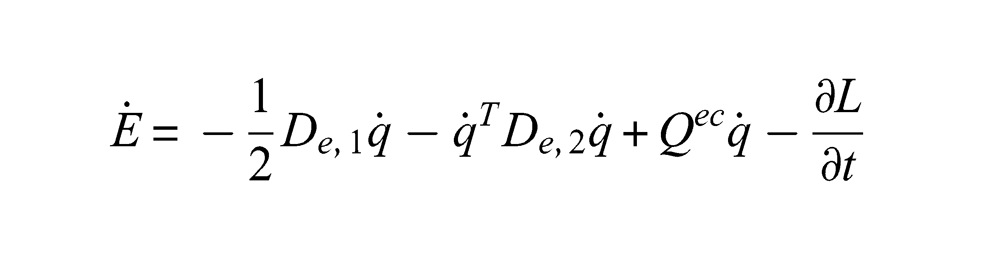
Corollary 4.1
where
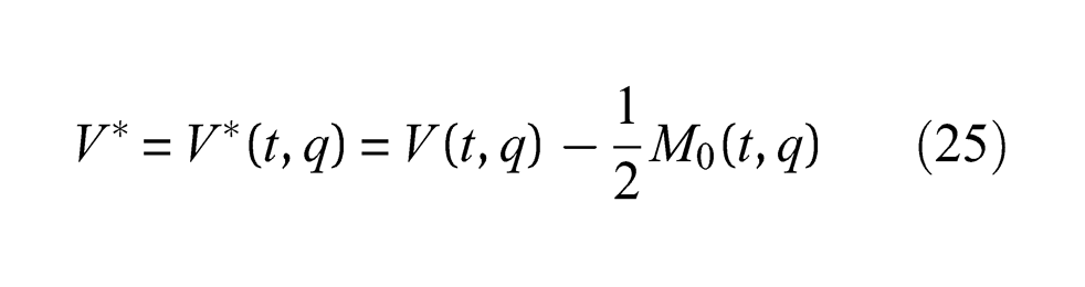
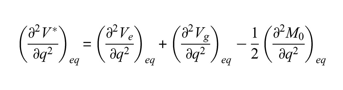
is the relative mechanical energy and
is called the modified potential energy of the multibody.
Proof: We have, according to (6)
and then
Invoking Proposition 4.3 one obtains (24). □
5. Linearization of the equations of motion
The equations of motion for the multibody are in this paper given by Equations (7) and (8).
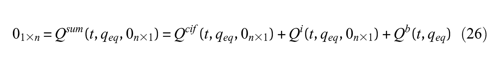
The multibody is said to be non-disturbed if the external force . A fixed configuration is an equilibrium configuration to a non-disturbed system if is a solution to (7) with and . If we insert into (7), one obtains the equilibrium equation:
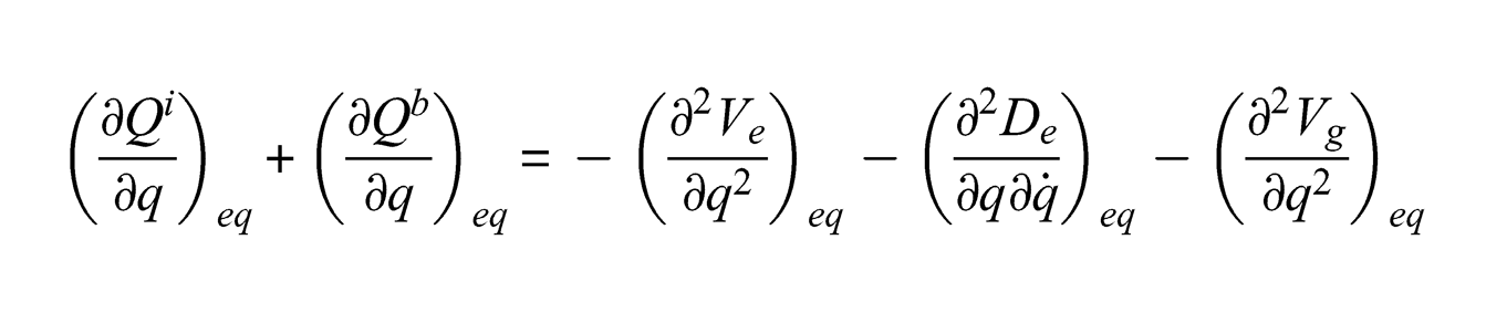
Proposition 5.1 If and are given by (14) and (15), respectively, then the equilibrium equation (26) may be written
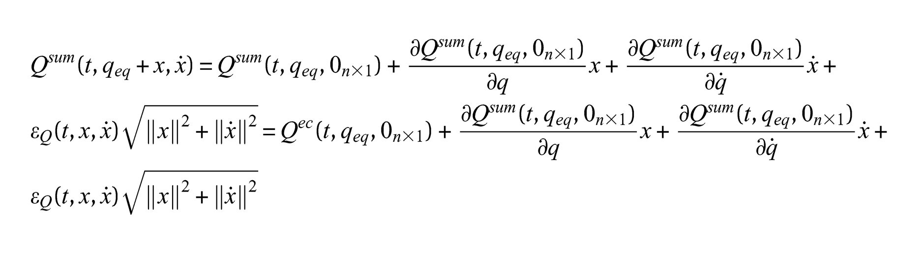
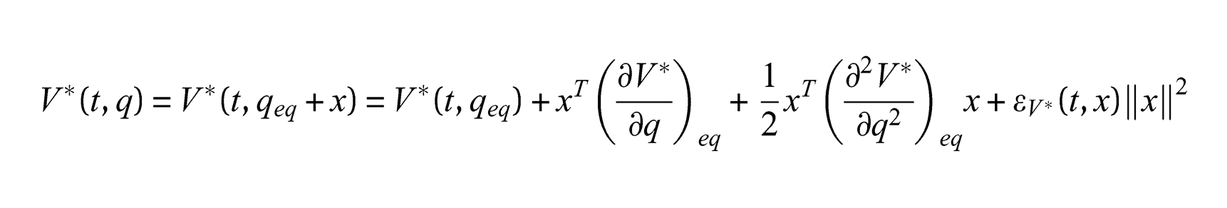
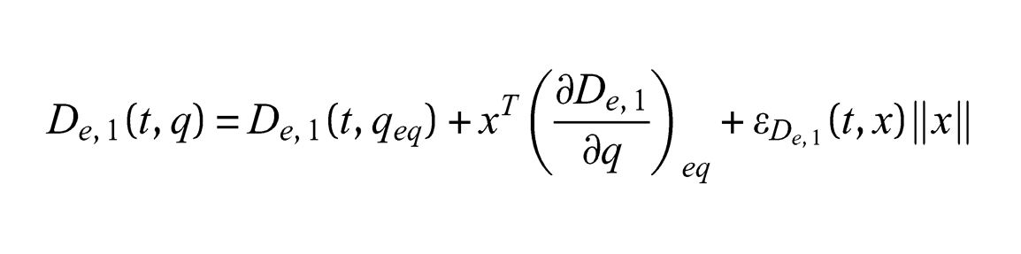
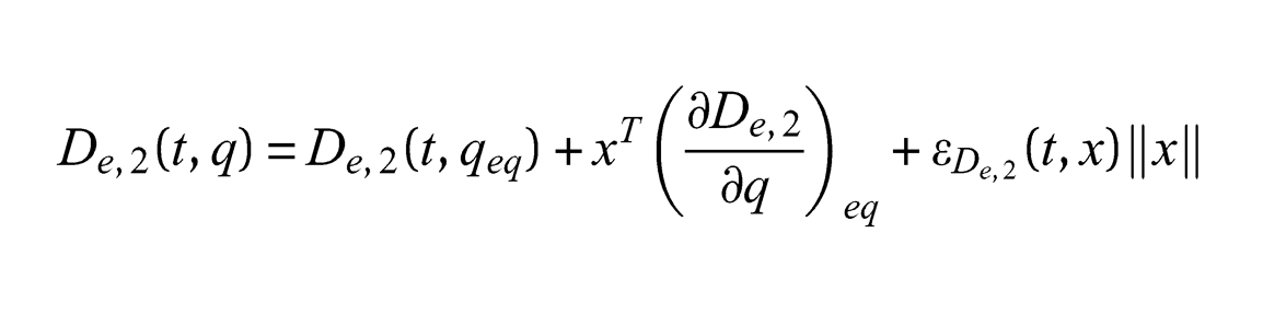
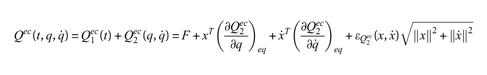
where now includes the external force and is given by (22). We have, using a Taylor expansion:
and is continuous at and . Furthermore
where is continuous at and . Thus
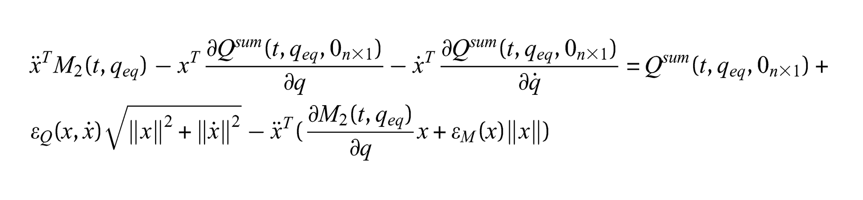
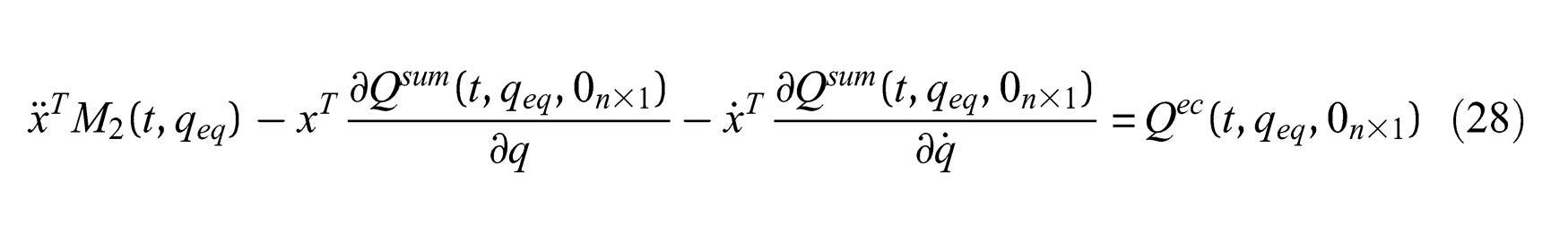
and from this we extract the linearized equations of motion:
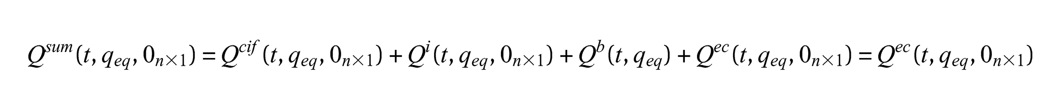
where we have used the fact that, according to (26):
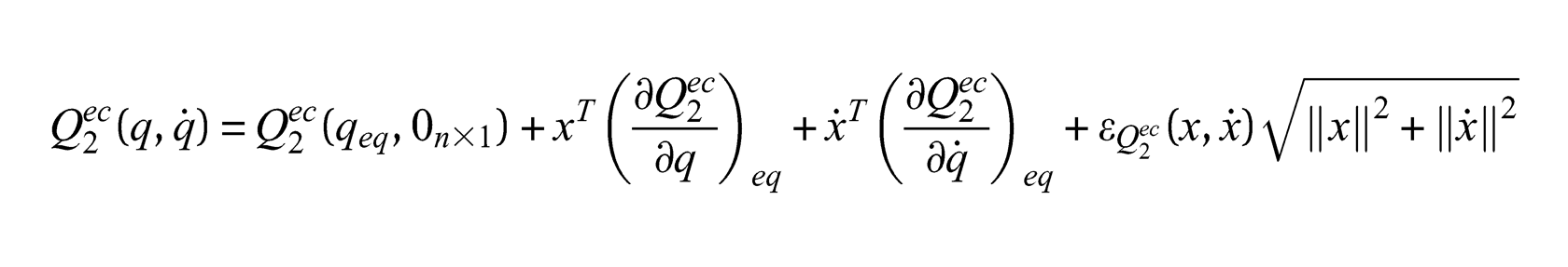
We have
where we have introduced the simplifying notation
From (9) it follows that
We now have the following.
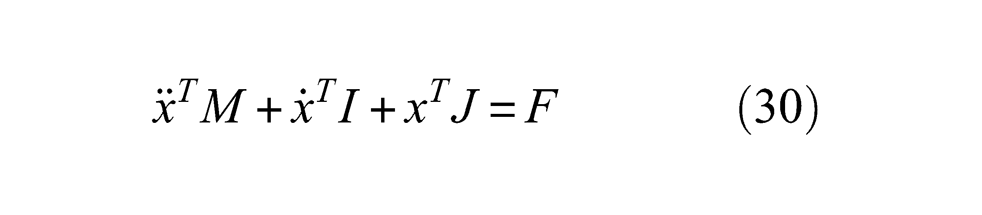
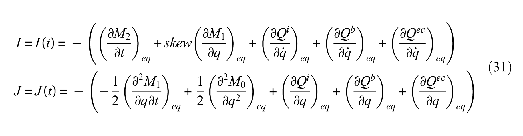
Proposition 5.2 The linearized equation of motion (28) may be written
where
and
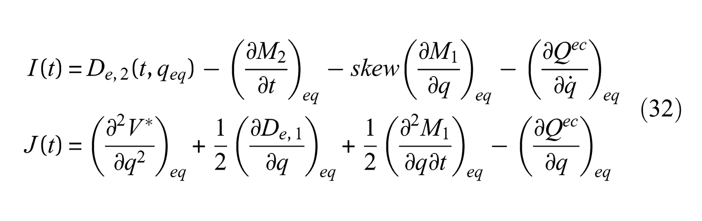
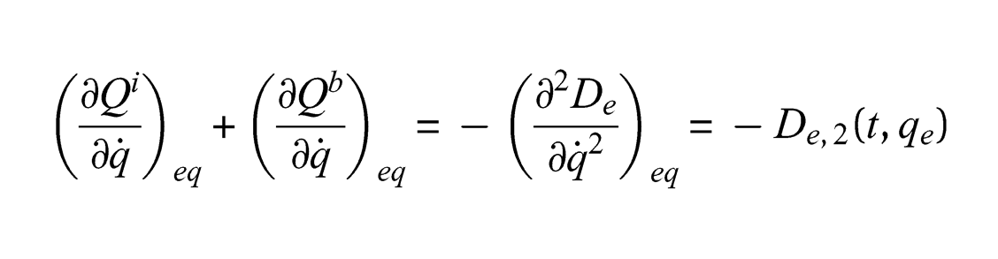
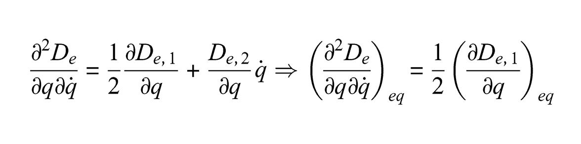
Corollary 5.1 If and are given by the assumptions (14) and (15), respectively, then
Proof: We have, according to (19):
since . Furthermore:
But and then
and this proves the corollary. □
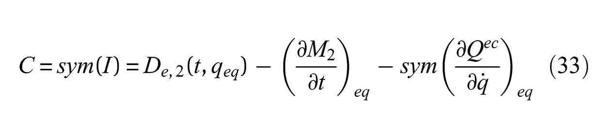
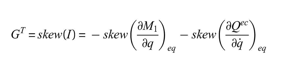
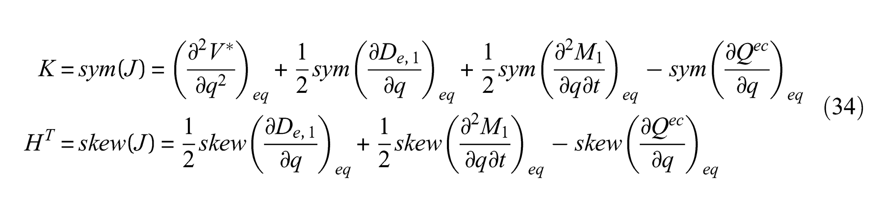
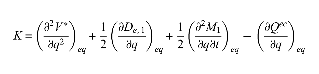
The matrix in (32) may be written where
Here is called the damping matrix and is called the gyroscopic matrix. The matrix may be written where
is called the stiffness matrix and is called the circulatory matrix. Note that
where
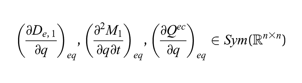
Corollary 5.2 If
then and
Proof: This is a direct consequence of (34). □
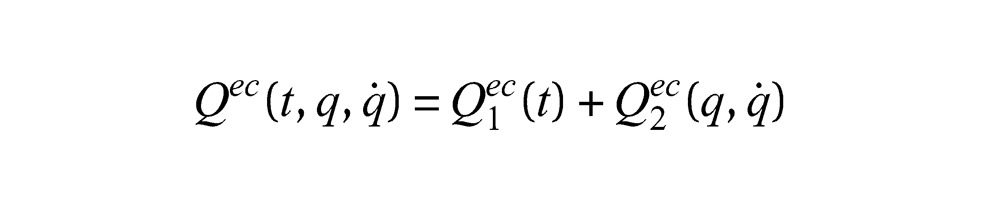
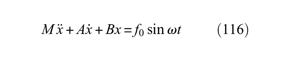
The coordinate system is called quasi-scleronomic if , , , , and are explicit functions of only, and not of . The external force is called quasi-scleronomic if
The external force then consists of two parts, one prescribed time-dependent part and one part depending on the state of the multibody. This second part may include so-called follower forces.
Remark 5.1: Traditionally, a coordinate system is called scleronomic if . In this case, , , , and, consequently, , .■
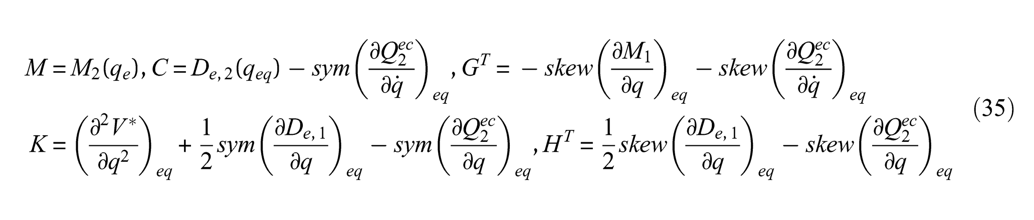
Corollary 5.3 If the coordinate system and the external force are quasi-scleronomic then
and
where now all matrices , , , and are constant matrices.
Proof: The expressions in (35) are direct consequences of (33) and (34). □
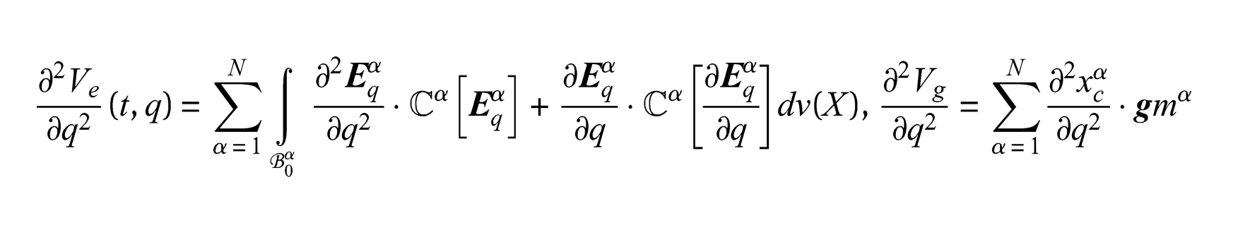
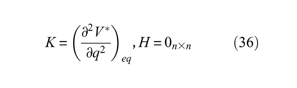
Corollary 5.4 If the coordinate system and the external force are quasi-scleronomic and
then
Proof: From (20) it follows that
This, together with (35)4,5, proves the corollary. □
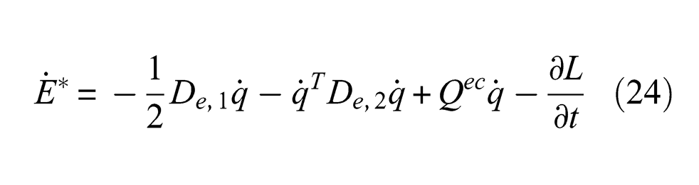
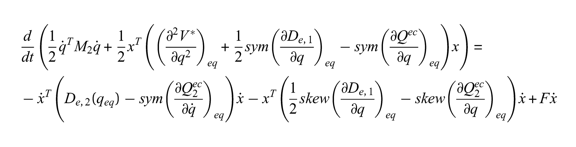
Introduce the linearized mechanical energy
Proposition 5.3 If the coordinate system and the external force are quasi-scleronomic, then the power theorem corresponding to the linearized equations reads
Proof: Considering the power theorem (24) we have the following Taylor expansion:
where the mapping is defined by
It satisfies and the mapping is continuous at and . Furthermore
where is continuous at and and
where the mappings and are continuous at , and . Finally
and then
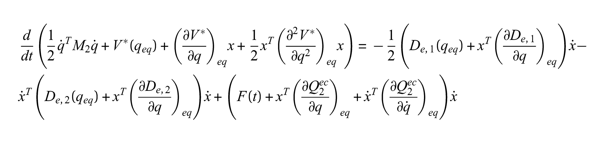
Inserting this into (24), and omitting higher order terms, one obtains
where we have used the fact that, in the present quasi-scleronomic case, . The previous equation is then equivalent to
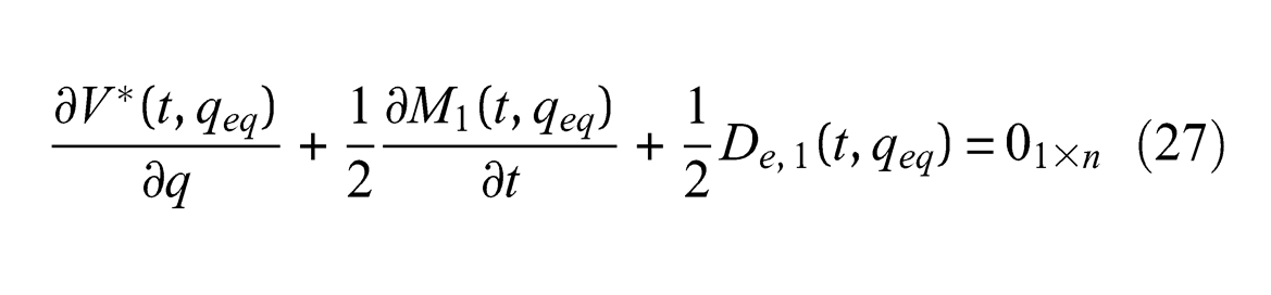
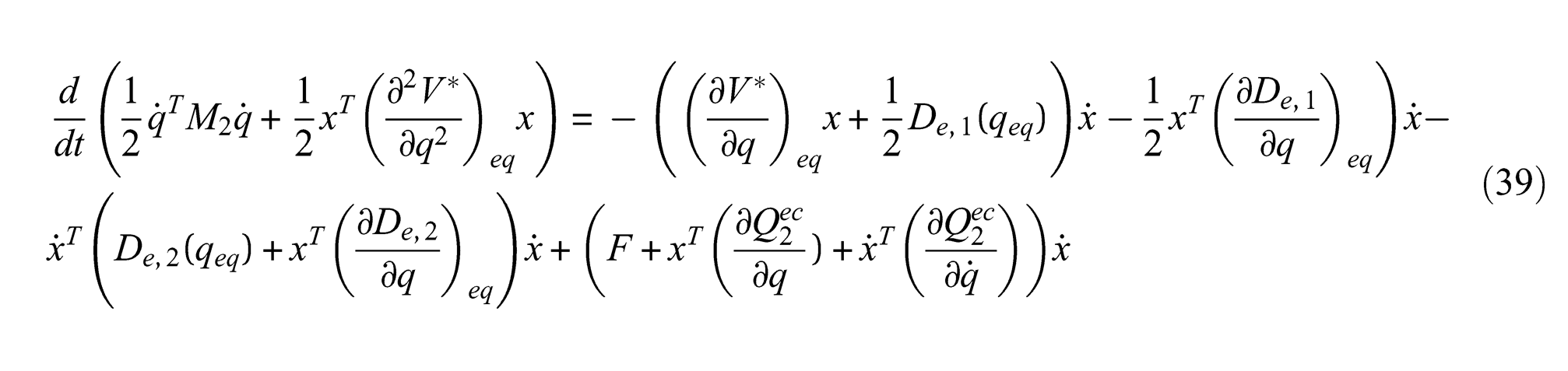
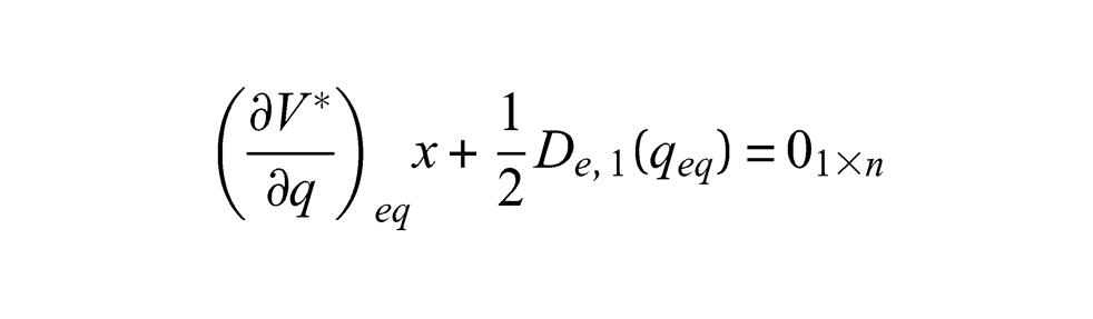
However, according to the equilibrium condition (27), we have
and then (39) may be written
and this proves the proposition. □
Remark 5.2: Multiplying equation (30) by from the right one obtains
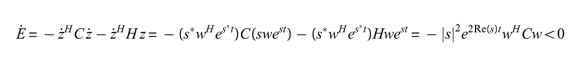
But and where is the linearized mechanical energy defined in (37). This inserted into the equation above results in the power theorem according to (38). If we accept complex valued solutions to (30) then the mechanical energy is defined by
where denotes the Hermitian transpose of (see Appendix A.1). Now assume that and , where and are constants. Then, since :
if is positive definite. Thus, the linearized mechanical energy is decreasing. More on this will be discussed in the forthcoming sections.■
6. The linearized equation
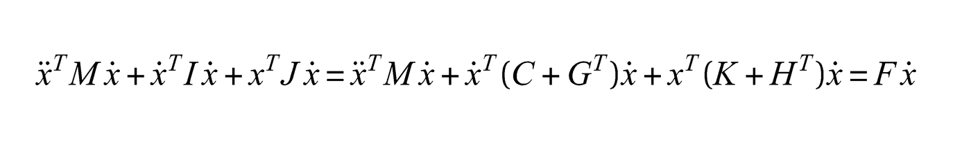
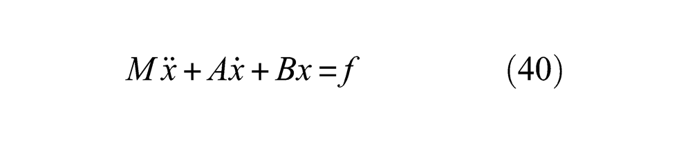
If Equation (30) is transposed one obtains the linearized equations of motion in the more familiar format:
where , and . We have and . Along with (40) one prescribes the initial conditions
where are given. A function satisfying (40) and (41) will, under certain conditions, represent a vibrational motion of the multibody in the neighbourhood of the equilibrium configuration. If the external force is identically zero the equation represents a free vibration of the system. Obviously, in this case and with , is a solution to the initial value problem representing the equilibrium solution.
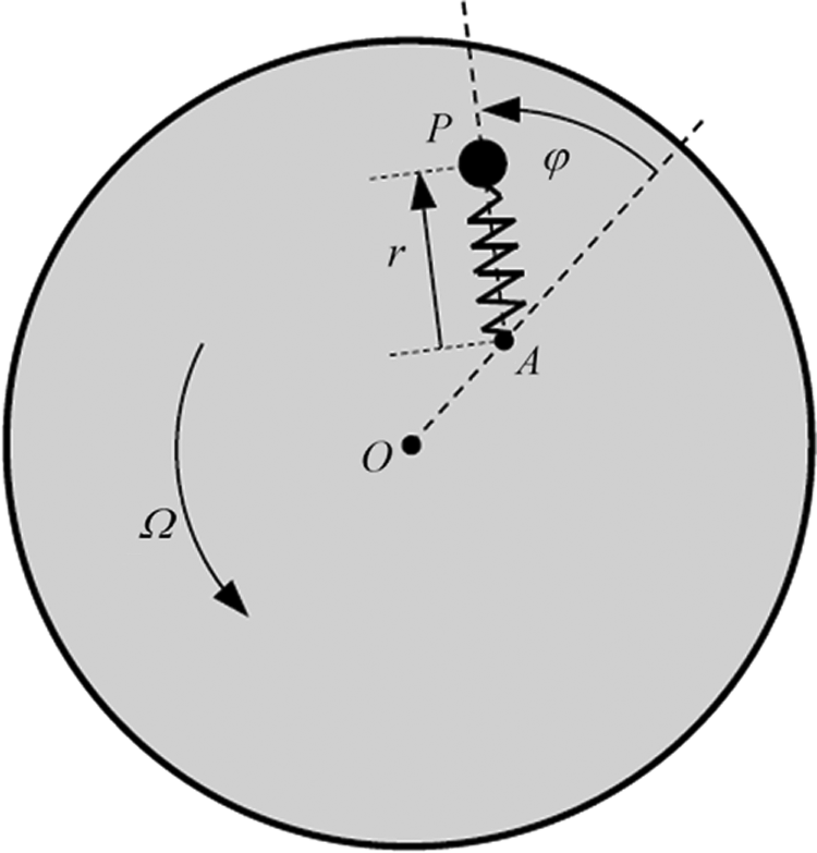
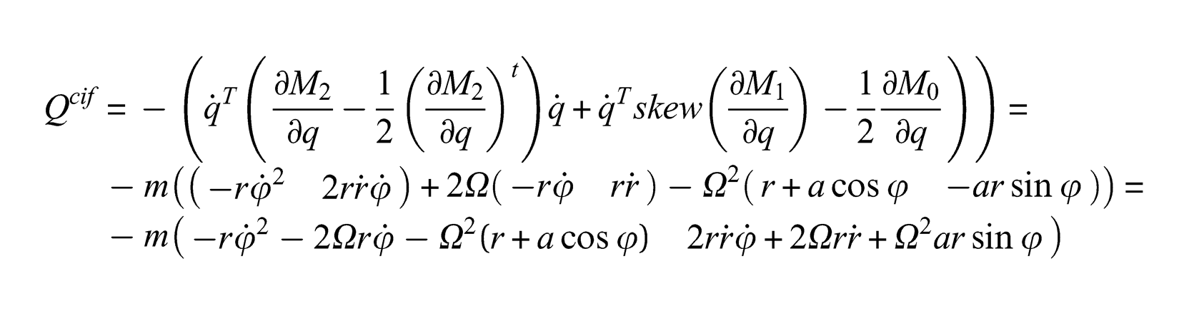
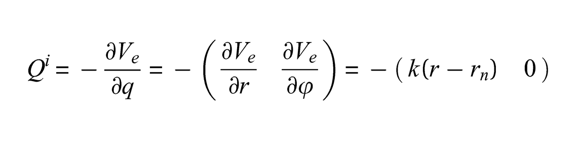
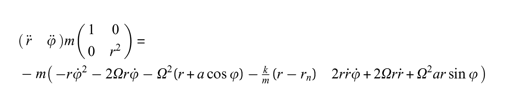
Example 6.1: A particle P with mass , which may slide without friction on a horizontal turn-table, is connected to a fixed point A on the table by an ideal linear elastic spring with spring constant and spring natural (unstressed) length (see Figure 1). The table is rotating around a fixed vertical axis through O with the prescribed constant angular velocity and its moment of inertia with respect to the axis is denoted by . Distance .
Two-dimensional multibody.
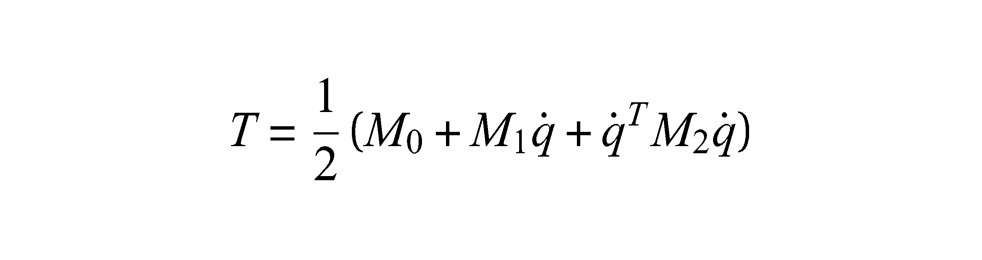
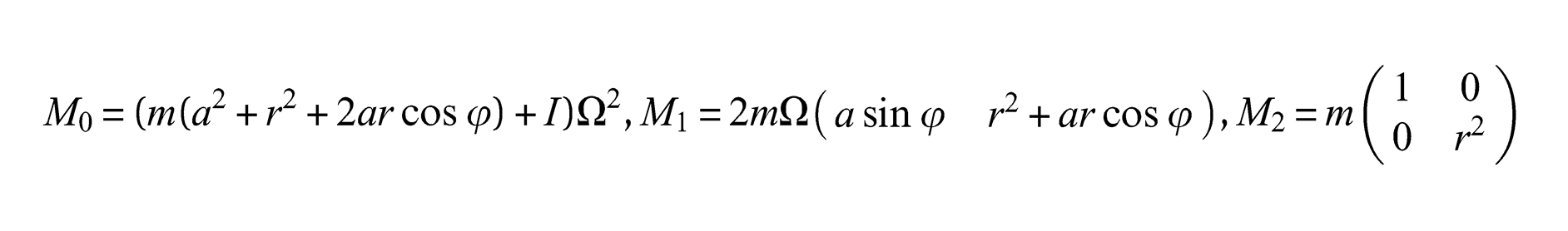
Introduce configuration coordinates according to Figure 1. The kinetic energy of the system
where and
The elastic potential energy is given by
The coordinate system used is thus quasi-scleronomic. We have
and
The equations of motion (7) and (22) read
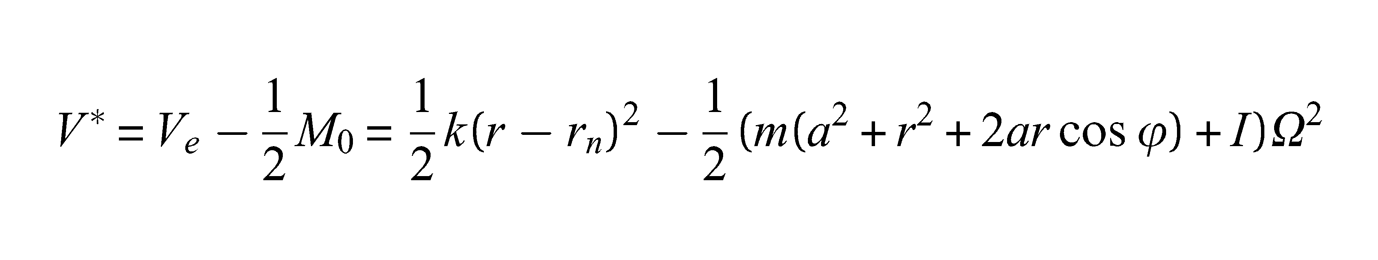
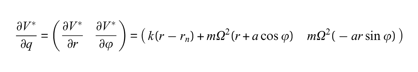
The modified potential energy is given by
and
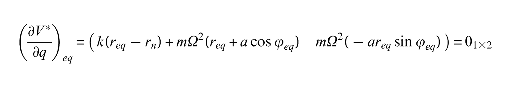
The equilibrium configuration is determined by Equation (27):
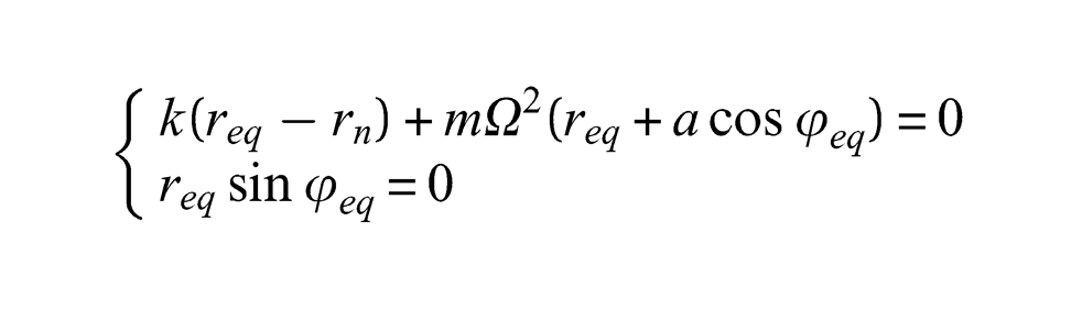
which is equivalent to
with a solution: . This corresponds to a stable equilibrium configuration.
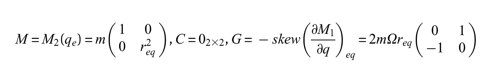
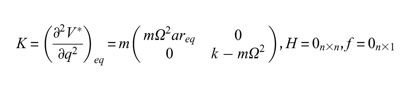
There may be another equilibrium configuration corresponding to , but this is then unstable. We introduce the configuration coordinate representing the deviation from the equilibrium solution. The linearized equations of motion are given by (40) where
In this case we have a non-zero gyroscopic matrix.■
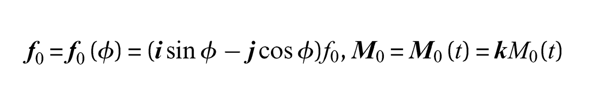
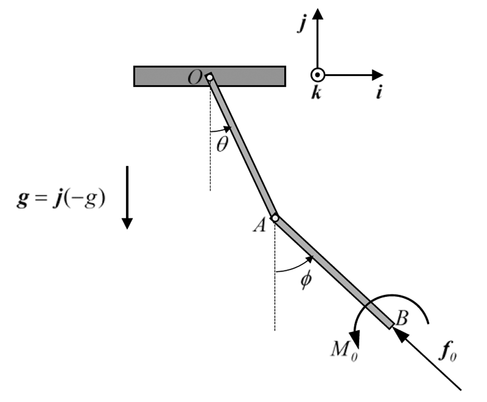
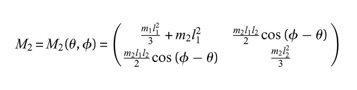
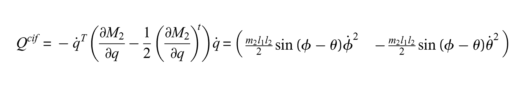
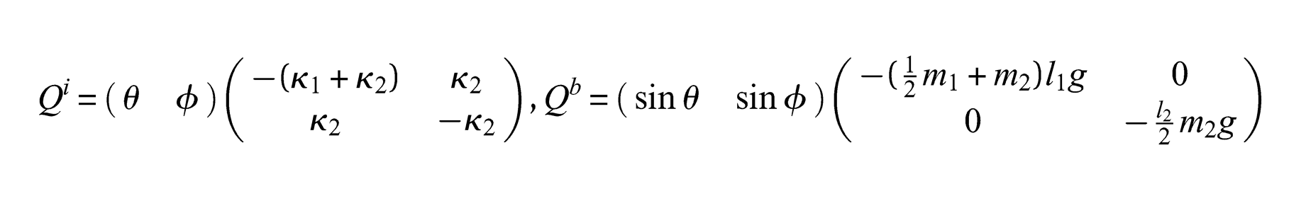
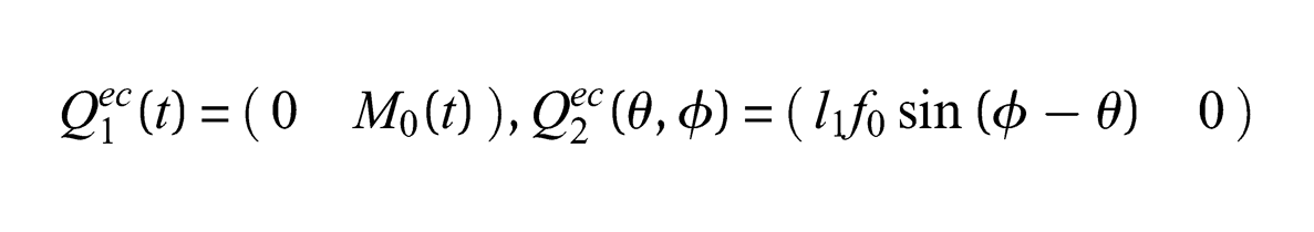
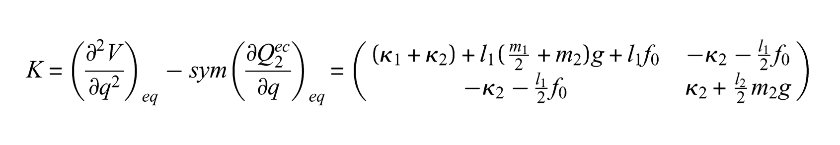
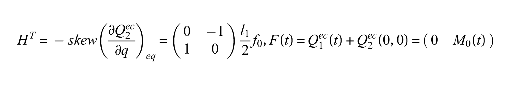
Example 6.2: The planar double pendulum consists of two homogeneous, rigid and slender bars OA and AB with masses and and lengths and , respectively. The bars are connected by an ideal revolute joint at point A and bar OA is connected, by an ideal revolute joint, to the fixed point O. The configuration space in this case is the two-dimensional torus. Configuration coordinates are introduced according to Figure 2. The pendulum is, at the joints at O and A, equipped with elastic torsional springs, with spring constants and , respectively. The pendulum is subjected to a follower point force and a point couple applied at the end-point B of bar AB and defined according to
where is a non-zero constant and is a prescribed function, being an orthonormal basis according to Figure 2. The pendulum may move in a vertical plane. The kinetic energy of the pendulum is given by
since and due to the scleronomic coordinate system.
The planar double pendulum subjected to a follower force and couple.
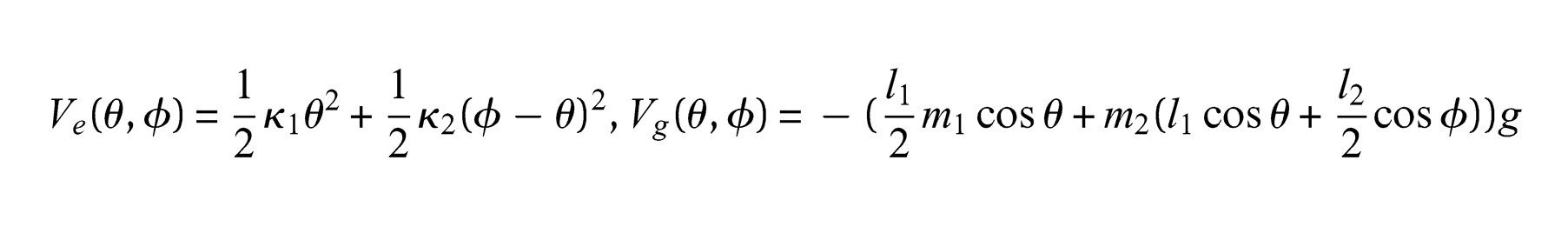
The potential energy of the pendulum may be written where
are the elastic and gravitational potential energies, respectively. The equations of motion for the pendulum read, according to (7) and (22):
where in this case
and
where
At the equilibrium configuration, given by , one has , and
In this case we thus have a non-zero circulatory matrix. There are three more equilibrium configurations corresponding to , , , and , , but these are unstable.■
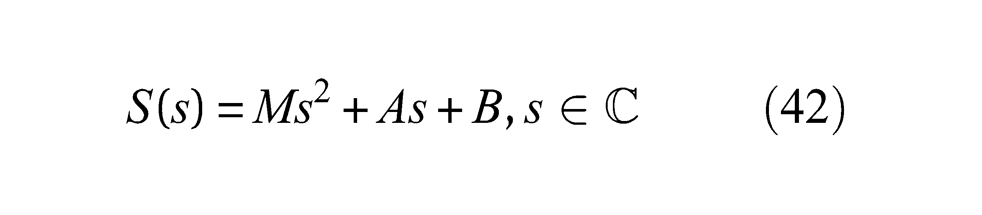
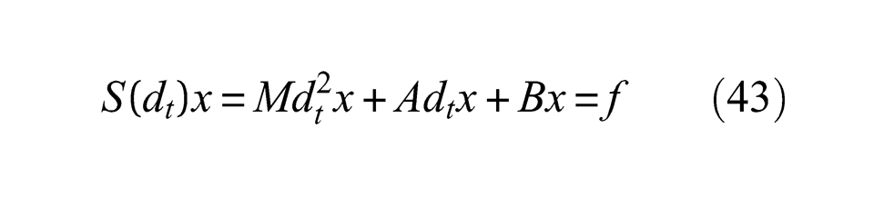
The matrix polynomial
is called the dynamic stiffness. The differential equation (40) may then be written ()
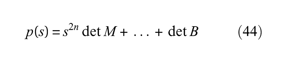
The characteristic polynomial, associated with the dynamic stiffness, is defined by . It has degree equal to and one may show that
where the intermediate terms have more complicated coefficients in terms of and .
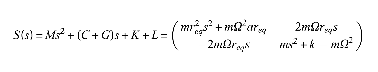
Example 6.1 (continued): The dynamic stiffness matrix of the system is given by
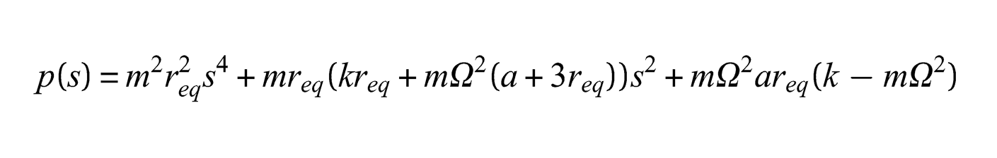
and the characteristic polynomial reads
■
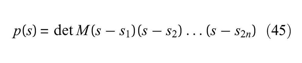
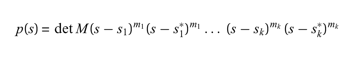
We assume, from now on, that is positive definite. Then . The spectrum, of the dynamic stiffness, is defined by . Note that . The characteristic polynomial may be factorized according to
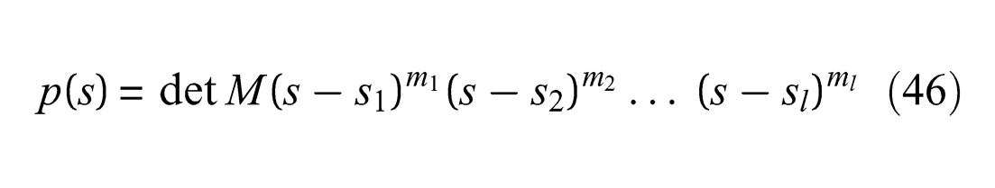
where . The characteristic polynomial has real coefficients and, consequently, if and only if . The roots of the characteristic equation may then be grouped into two sets and , where . Note that the number of real roots must be even and that some of the may be equal. The number of times the root appears in (45) is called its (algebraic) multiplicity and denoted (. We may write
where now all are distinct complex numbers and .
The following well-known result will be frequently used in the forthcoming discussions.
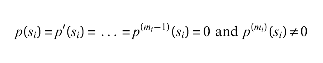
Lemma 6.1 is a root of the characteristic equation with multiplicity if and only if
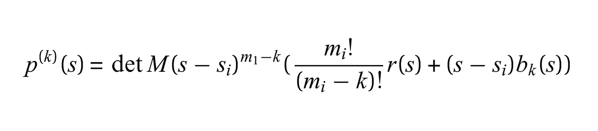
Proof: is a root with multiplicity if and only if , where is a polynomial with and . Now if then
where is a polynomial with . Then and
This proves the lemma. □
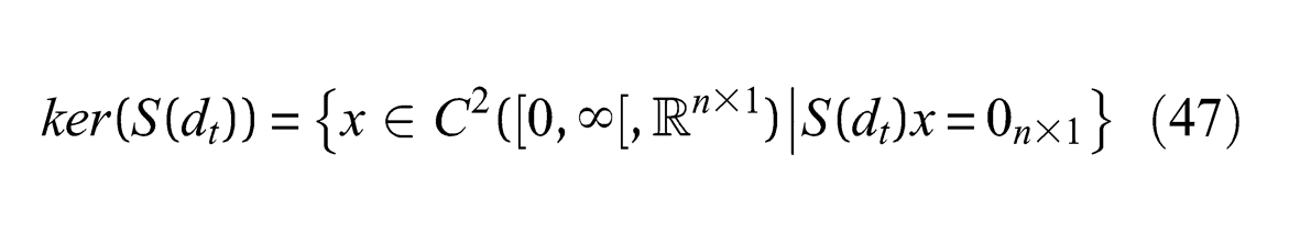
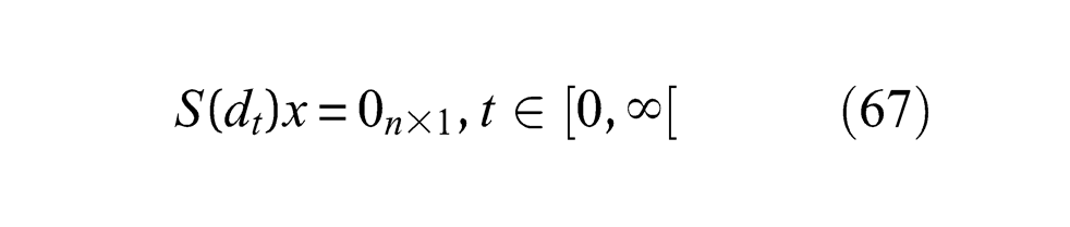
With . we introduce the linear spaces:
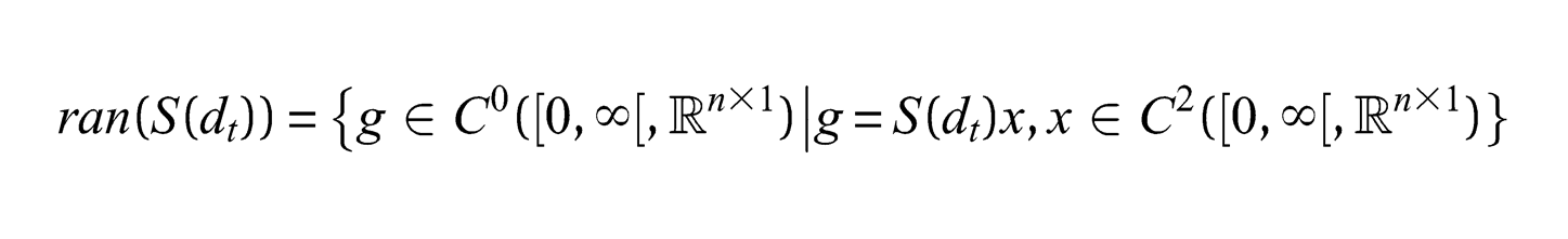
The kernel (null-space) and range of the linear differential operator :
are given by
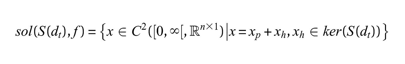
For we define and we then have the following trivial implications: and , . Thus we have the following.
Proposition 6.1 Let (a particulate solution). Then
Theorem 6.1 (Existence and uniqueness) The initial value problem
has a unique solution .
Proof: By introducing , where , Equation (43) may be written , where and
Note that . The function is affine and the theorem now follows from general theorems on existence and uniqueness for first-order ordinary differential equations (see, for instance, Arnold [5]). □
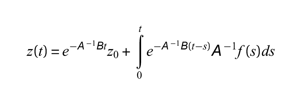
Remark 6.1: A formal solution of the initial value problem is given by (see Arnold [5])
The character of this solution is determined by the Jordan canonical form of the matrix . This approach is mathematically efficient but it lacks some of the physical transparency obtained by directly considering the solution to Equation (43).■
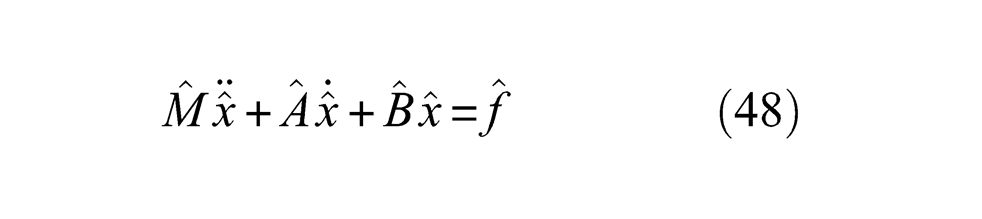
Remark 6.2: A linear change of coordinates is obtained by the relation , where is a constant, non-singular matrix. Equation (40) is then equivalent to
where , , and . Note that and , . A coordinate change results in the dynamic stiffness . The corresponding characteristic polynomial is given by . Thus . A decoupling of the equations in (40) is obtained if one can find a change of coordinates that renders the matrices , and diagonal. In this case the solution of (48) is more or less trivial. It is well known that if and are symmetric (non-gyroscopic and non-circulatory system) and if then there exists a change of coordinates that decouples the equations (Caughey and O’Kelly [9]).■
The result in Proposition 7.1 implies that if one has found solutions to the differential equation and can show that these are linearly independent then, by combining them linearly, all solutions have been found. When searching for these solutions it is a good strategy to look among the very regular functions, that is, functions belonging to the space of infinitely differentiable functions, that is, assuming .
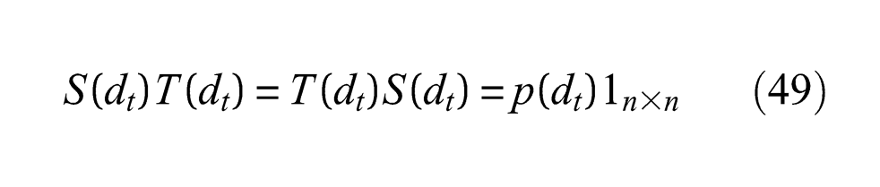
Introduce the adjoint differential operator related to and defined by . (See the Appendix for the algebraic definition of the adjoint.) We have
where
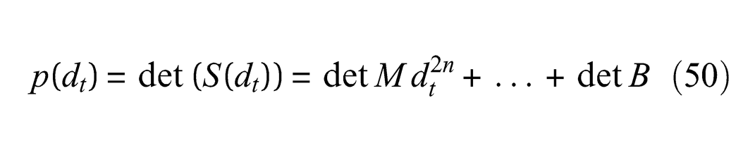
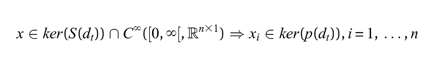
The kernel of the differential operator is given by . The equation is called the characteristic differential equation. A direct consequence of (49) is the following.
Proposition 7.2
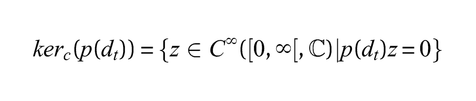
In order to answer the question of the dimension of it turns out to be advantageous to complexify the problem and consider
Note that if and only if , where , and since the operator has real coefficients it follows that and , where is the complex conjugate of .
The main theorem, characterizing members of , is the following.
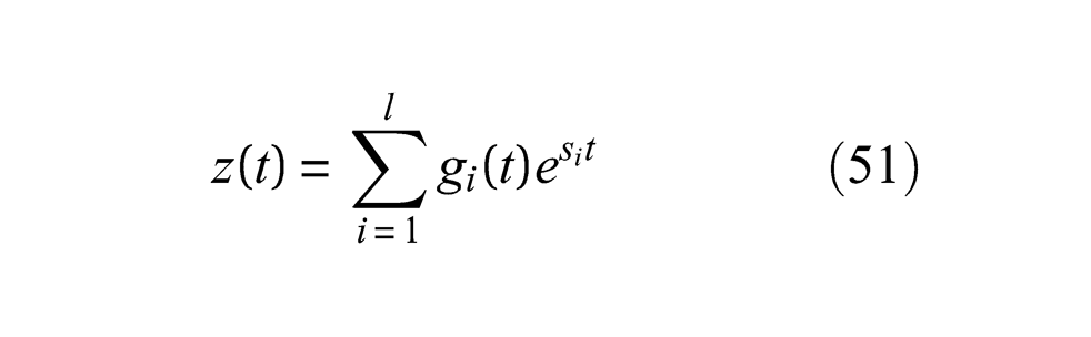
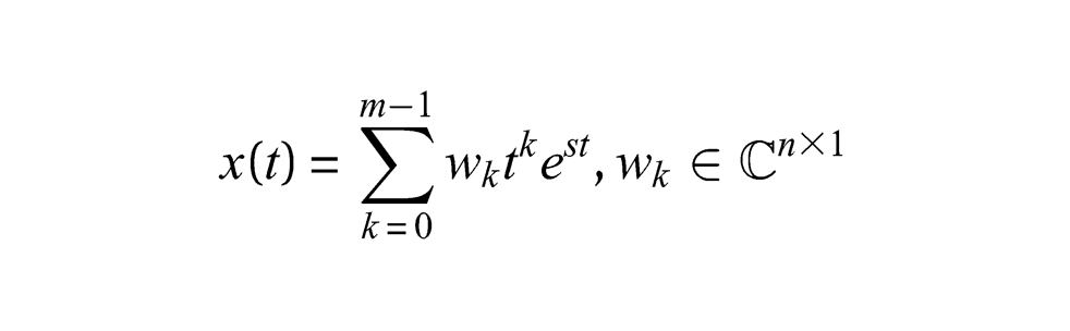
Theorem 7.1 If the characteristic equation has the distinct roots with multiplicities , (), then a solution to the characteristic differential equation is given by the exponential-polynomial (expol):
where are polynomials with complex coefficients and .
Proof: A proof of this may be found in a textbook on ordinary differential equations, for instance Birkhoff and Rota [5] (Chapter 3). A proof, complying with the notation used in this paper, is given in Appendix A.3.2.□
The following conclusion is a direct consequence of the previous theorem.
Corollary 7.1.
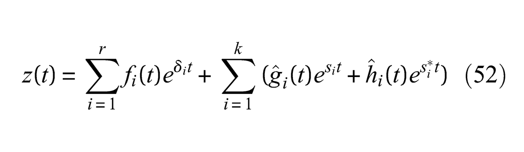
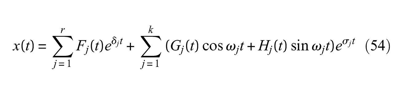
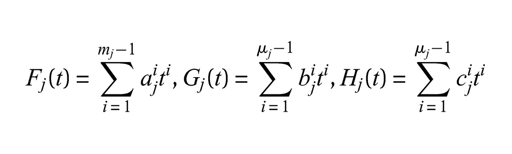
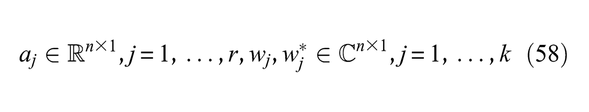
The roots of the characteristic equation may be grouped into two sets and with multiplicities and , where and . The expol (51) may then be written
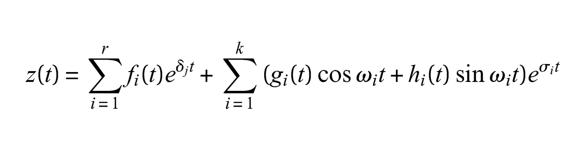
where , and are polynomials with complex coefficients and , . Put , where is called the damping factor and is called the (damped) natural frequency. The expol (51) may then be written
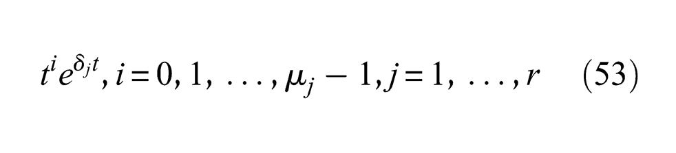
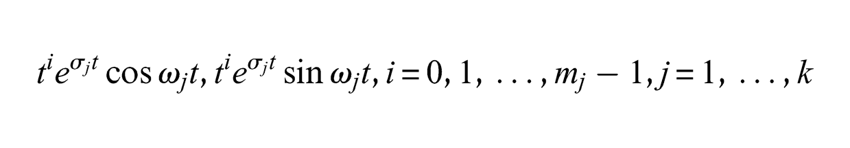
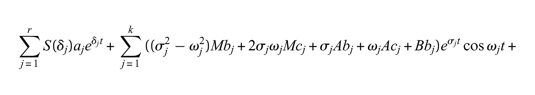
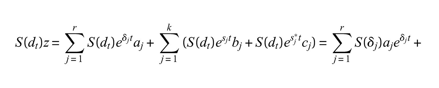
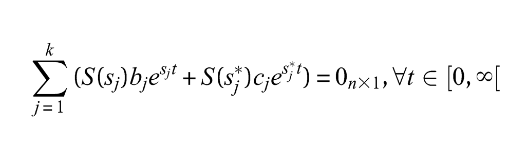
where . Obviously, if we are only interested in real valued expols we may choose polynomials with real coefficients. It is clear that the functions
are linearly independent over . We have thus demonstrated that and that contains exponential and harmonic functions combined with polynomials. Are there other functions in ? The answer to this question is, no! Before we prove this we return to our original problem, namely, the structure of . We know that and that if then . As candidates for elements in we now take
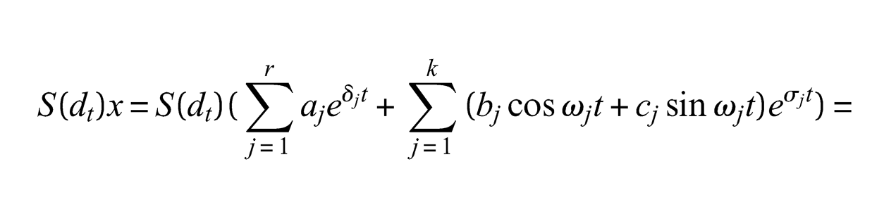
where
and are constant column matrices. These functions span a linear space of dimension equal to . If then , according to (54), belongs to , then there must be a certain relationship between the vectors , and . This relationship is established by the condition .
8. Simple roots to the characteristic equation
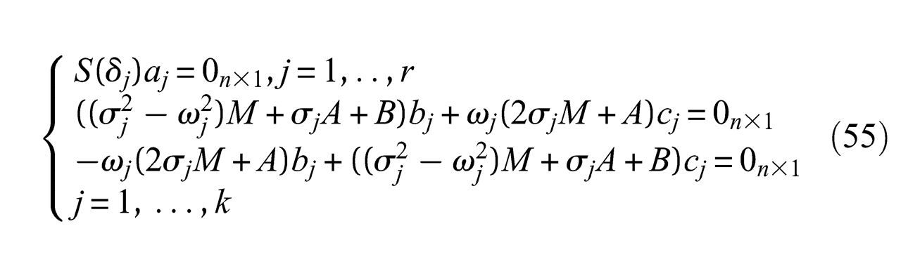
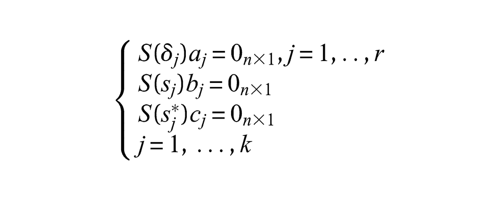
Assume that all roots of the characteristic equation are simple, that is, and . Then , and , where are constant vectors. Consequently
where and . Then
which is true if and only if the vectors , , satisfy the equations
If instead one uses complex expols
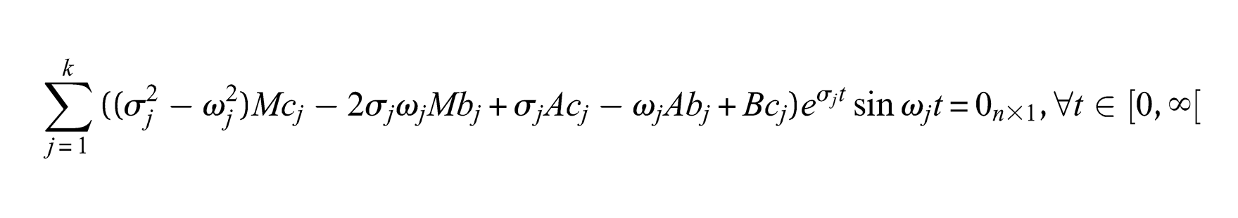
where now , , , then
which is true if and only if the vectors , , satisfy the equations
These conditions appear much simpler than the (equivalent) ones given in (55), this being a beneficial consequence of complexification. Thus for each one should determine so that
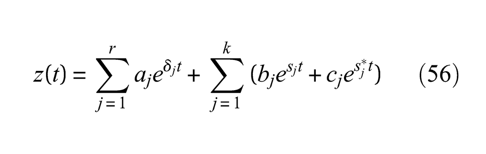
which means that we are now looking for the kernel . Obviously, . If then there exists a vector satisfying (57), that is, . The column matrix is called the eigenvector corresponding to the eigenvalue. With the notation
and we have . Note that if we may choose and then . Now assume that
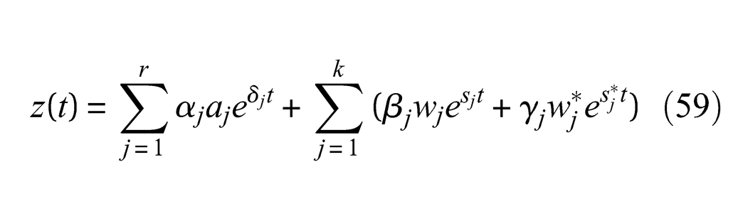
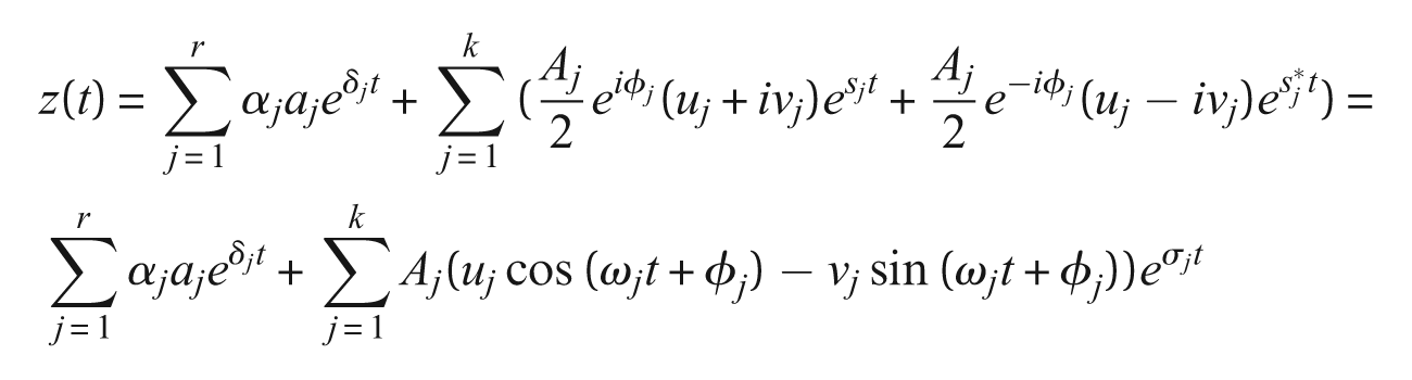
are solutions to (57) corresponding to , and , respectively. Then (56) may be written
where . The expression (59) contains arbitrary complex constants. Note that the column vectors in (59) are linearly dependent. The expression is real valued if and only if , .
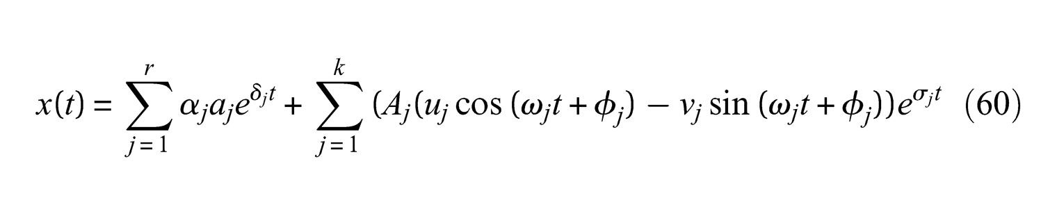
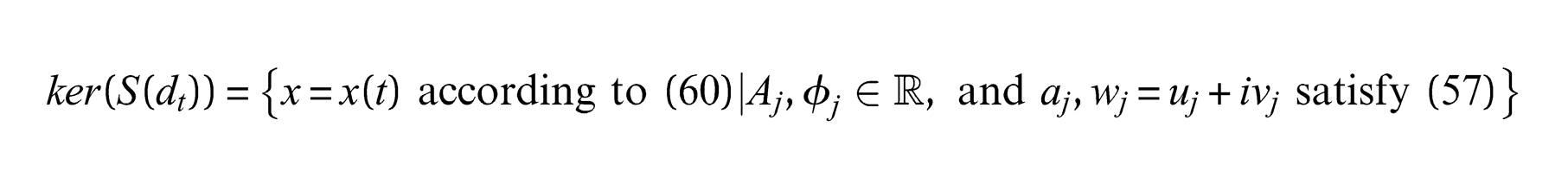
Proposition 8.1 Real valued solutions to of the expol type are given by
where and satisfy (57).
Proof: We may write and and . Then (59) may then be written
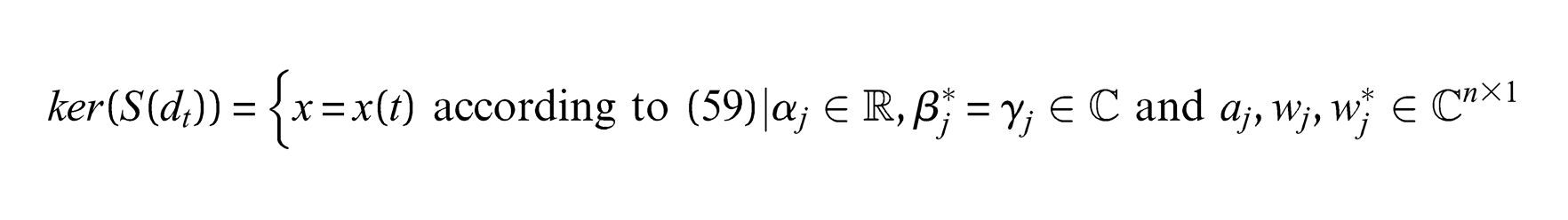
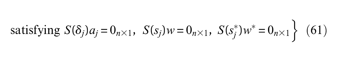
Theorem 8.1 If the roots of the characteristic equation are simple then
Proof: Note that , according to (60), contains arbitrary constants: , and . Thus these functions constitute a linear space with dimension . However, according to Proposition 7.1, and this proves the theorem. □
Remark 8.1: We have the following alternative representation of :
■
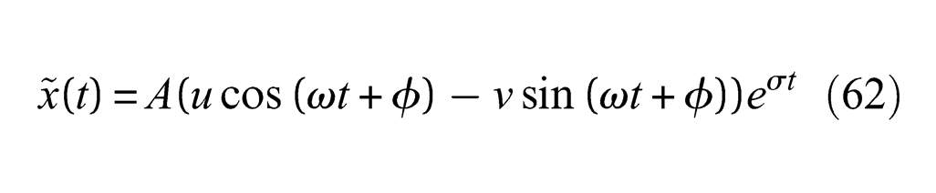
The oscillating terms in (60) are on the form
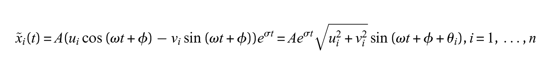
This is called the complex natural mode with (damped) natural frequency and damping factor. With the expression (61) represents, for fixed , an oscillating motion with exponentially decreasing amplitude. Component-wise we have
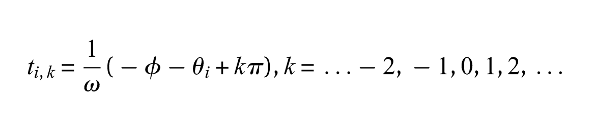
where . The mode component is equal to zero at times
These times are in general depending on the specific mode component . However, if , independent of then the mode components will be equal to zero simultaneously. In this case
and then
This is called a real (natural) mode. Note that and with one obtains and .
Remark 8.2: Real natural modes are present in many multibody systems. If , (non-gyroscopic and non-circulatory) and if then all modes are real. This situation is, for instance, at hand in the case of proportional damping where it is assumed that , where and (see Clough and Penzien [13]).■
The following corollary is an immediate consequence of Theorem 8.1.
Corollary 8.1 If the characteristic equation has simple roots then
Proof: We have . Now assume that for some one has , then it follows by inspection of (60) that , which contradicts the fact that, according to Proposition 7.1, . Note that given constant, linearly independent vectors and , then the functions are linear independent functions over in the space .
This proves the proposition. □
We now summarize the discussion above by giving the following well-known scheme for solving the equation .
Set up the dynamic stiffness .
Calculate the characteristic polynomial .
Determine the roots of the characteristic equation . It is assumed that all roots are simple.
Determine so that .
Insert and into (60).
In the present case of simple roots we may read off the solution in step (iv) directly from the adjoint matrix to the dynamic stiffness: We have
Proposition 8.2 If is a simple root to the characteristic equation then and (in step (iv) above) may be taken as proportional to any non-zero column vector in the matrix .
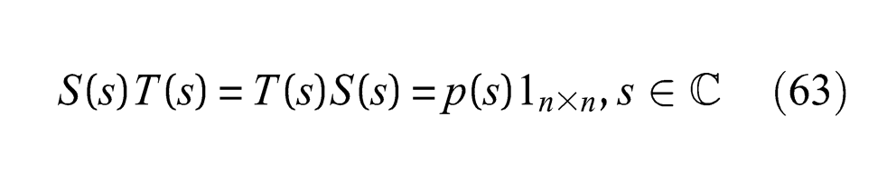
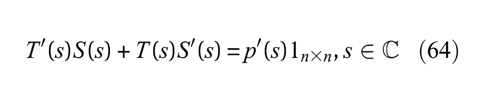
Proof: From relation (63) one obtains the implication . Let , where is the ith column in the matrix . Then . Thus, every is an eigenvector. The existence of at least one column vector follows from the assumption that is a simple root. By differentiating (63) with respect to , it follows that
and then
Now if then
since, according to Lemma 6.1, . From this we conclude that . This proves the proposition. □
Remark 8.3: If more than one column in is non-zero, let us say and , then these columns must be linearly dependent.■
If the characteristic equation has simple roots then the function , satisfying the initial conditions , is determined by the conditions
or in matrix format
where
The real constants , and are uniquely determined by (65). This follows from the uniqueness theorem, Theorem 6.1. The matrix is thus non-singular. Note, however, that the vectors must be linearly dependent. For special properties of the coefficient matrices and in (40) the modes will fulfil certain orthogonality properties that will simplify the solution of (65). This is, for instance, the case for the system defined in Remark 8.2 above. In this case we have real modes and orthogonality properties according to Corollary 8.5 below.
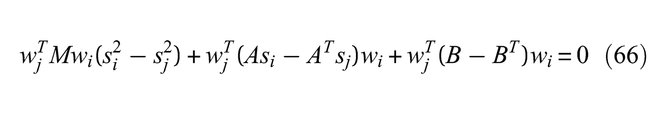
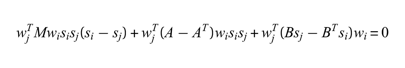
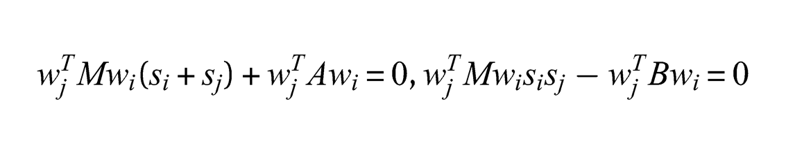
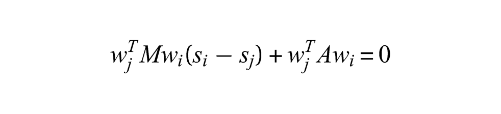
Proposition 8.3 If and , then
Proof: We have, since :
Furthermore
Subtracting these expressions pairwise gives (66). □
The following corollaries are direct consequences of the previous proposition.
Corollary 8.2 If and if then
Corollary 8.3 If then, if and , :
Corollary 8.4 If then, if and , :
Corollary 8.5 If and if the modes are real then, if , and , :
Proof: With , one obtains from (66)1
and then from (66)2. □
Remark 8.4: The previous corollary contains the classical orthogonality conditions obtained by assuming Rayleigh damping, that is, , and , where (see Lord Rayleigh [1]).
9. Multiple roots
The appearance of multiple roots in a multibody system is often a consequence of some symmetry of the system. Systems with multiple roots are, however, sensitive to disturbances. They may, from the point of view of applications, often be considered as a ‘degenerated’ limit case that may be done away with by arbitrarily small changes of the coefficient matrices and . Nevertheless it seems important, also from the engineering point of view, to be aware of some of the consequences of the presence of multiple roots. Investigations of multibody systems with general coefficient matrices and and with multiple roots are, however, sparse in the engineering literature. One of the few references we have found is Wu and Greif [14], where a vibrating system with null as well as non-null eigenvalues is analysed.
The algebraic multiplicity of a root to the characteristic equation will, in general, give rise to mathematical as well as numerical complications. Let be a root of the characteristic equation with algebraic multiplicity . The geometric multiplicity of is defined by . It is always the case that . An eigenvalue is called defect if . It is the presence of defect eigenvalues that makes the situation for multiple roots more complicated than for simple roots. Note that, in the case of simple roots, it follows from Corollary 8.1 that .
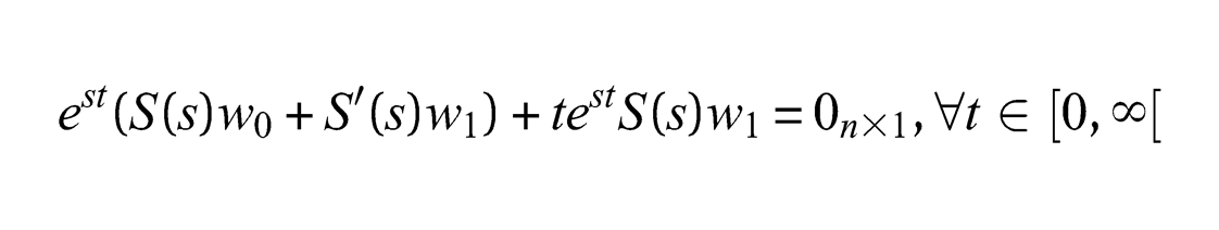
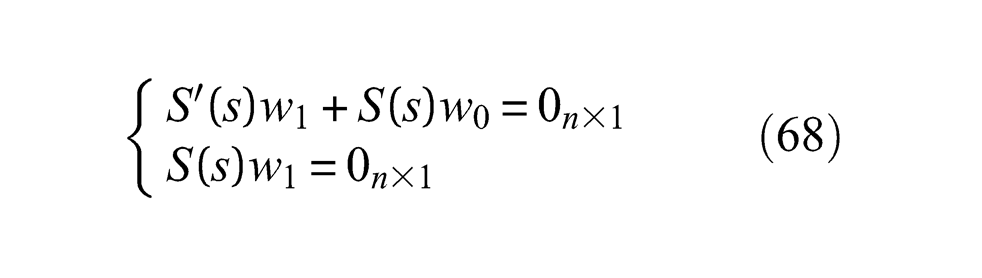
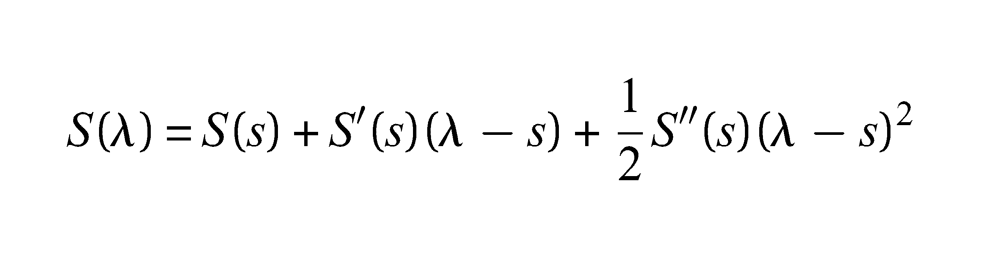
If is a double root to the characteristic equation then if and only if
where
Thus (67) is equivalent to
which is equivalent to the conditions
Note that since there always exists a vector such that and then , is a solution to (68), called the trivial solution. A non-trivial solution is obtained if .
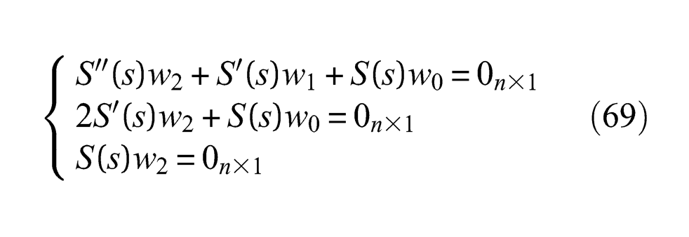
If is a triple root to the characteristic equation then if and only if
This may be generalized according to the following.
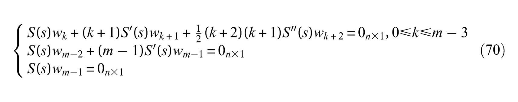
Theorem 9.1 If is a multiple root to the characteristic equation with multiplicity , then the function
is a solution to (67) if and only if
For the proof of this theorem we need the following.
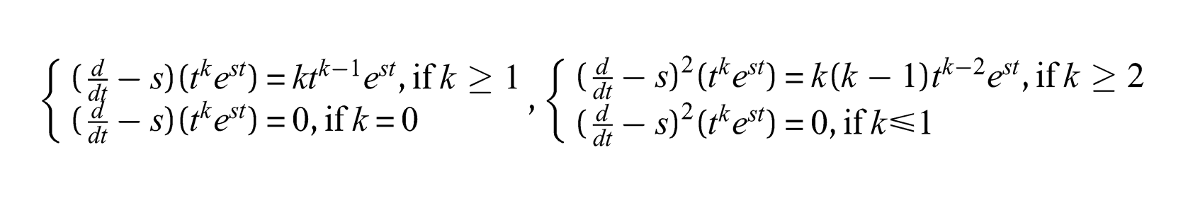
Lemma 9.1
Proof: Follows by a straightforward computation. □
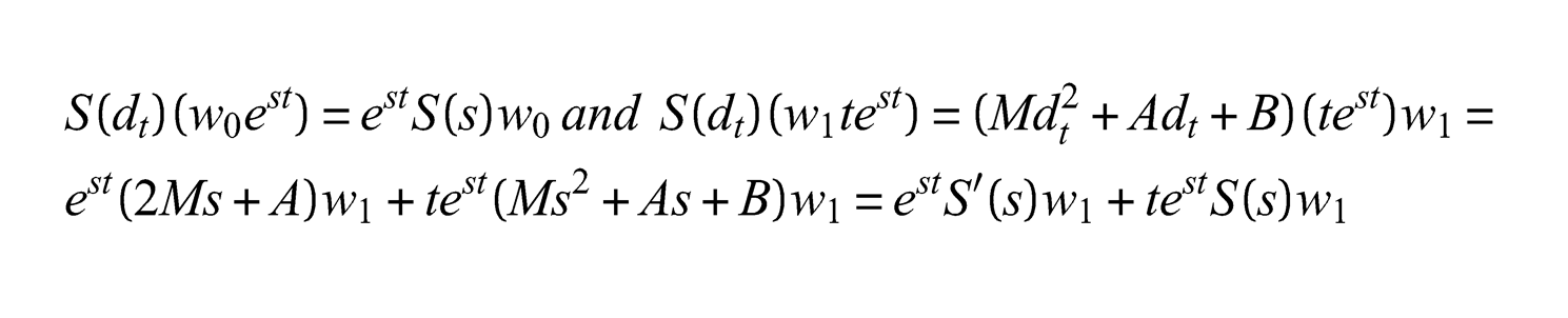
Proof: (Theorem 9.1) We have, for :
By replacing with one obtains
and then
This expression, together with Lemma 9.1, results in
Thus
and this is equivalent to (70). □
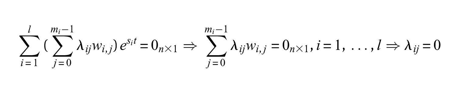
If there always exists a vector such that . A trivial solution to (70) is then given by , . Equations (70), with the requirement , define a generalized eigenvalue problem where are called generalized eigenvectors. A sequence of vectors () satisfying (70) is, in the mathematical literature, referred to as a Jordan chain for of length (see Gohberg et al. [15]). Note that some of the vectors in the chain might be equal to zero.
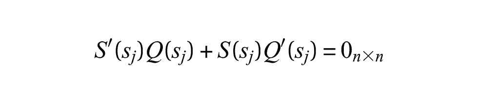
If is a double root to the characteristic equation then, according to Lemma 6.1, , and . It then follows that
Now let and , where , . Assume that for some . Then , constitute a Jordan chain. If then for some , since by differentiating (63) twice one obtains
and then if
A trivial solution to (70) is then given by , . This procedure may be generalized to a root with multiplicity .
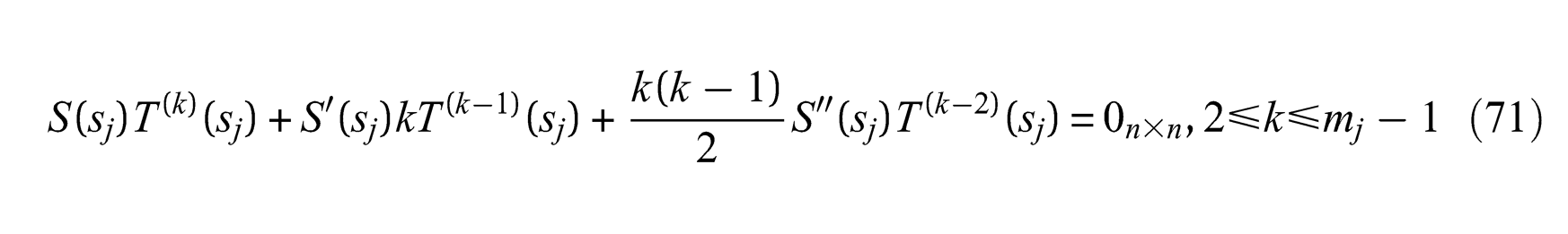
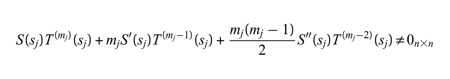
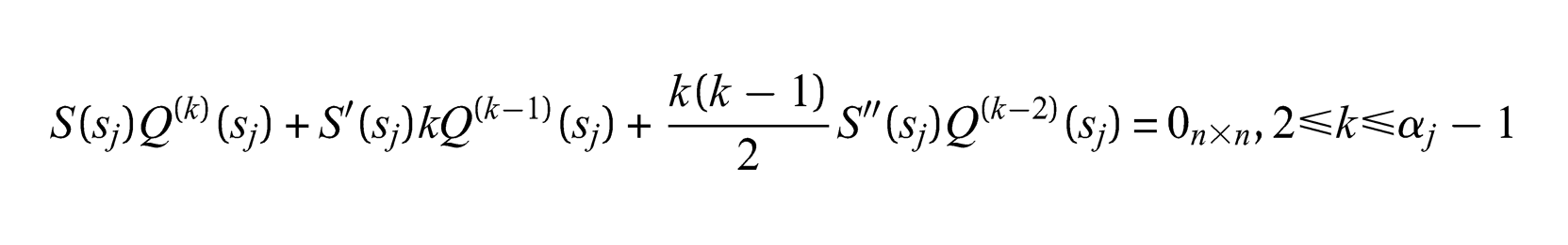
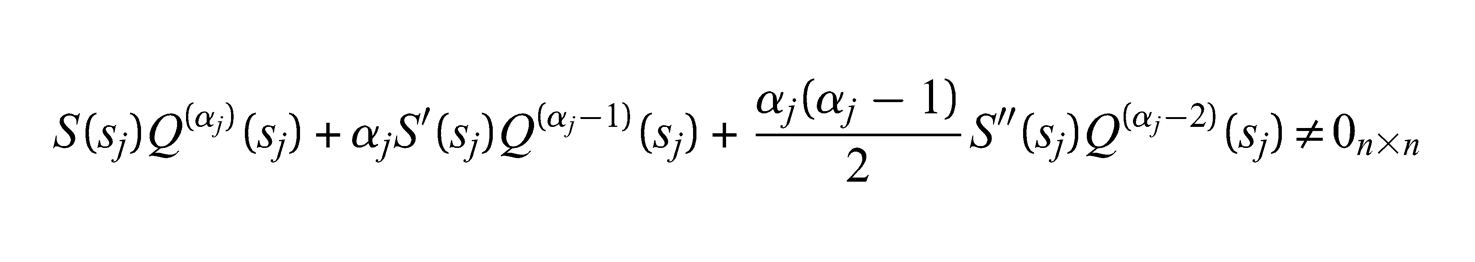
Proposition 9.1, with multiplicity , if and only if
Proof: By differentiating the identity (63) times one obtains
For this results in
For , using the Leibnitz formula, one obtains
since for . The proposition now follows from Lemma 6.1. □
The structural similarity between Equations (70) and (71) is apparent and suggests a possibility of using the adjoint in the solution of the generalized eigenvalue problem.
Remark 9.1: Note that by changing the order of and one obtains
and thus conditions (71)4 is equivalent to
■
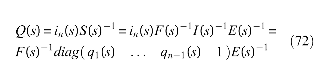
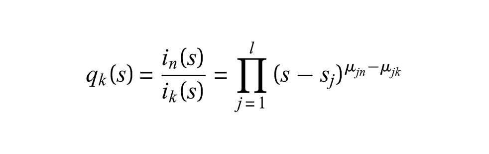
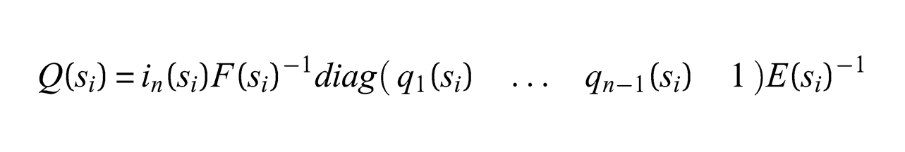
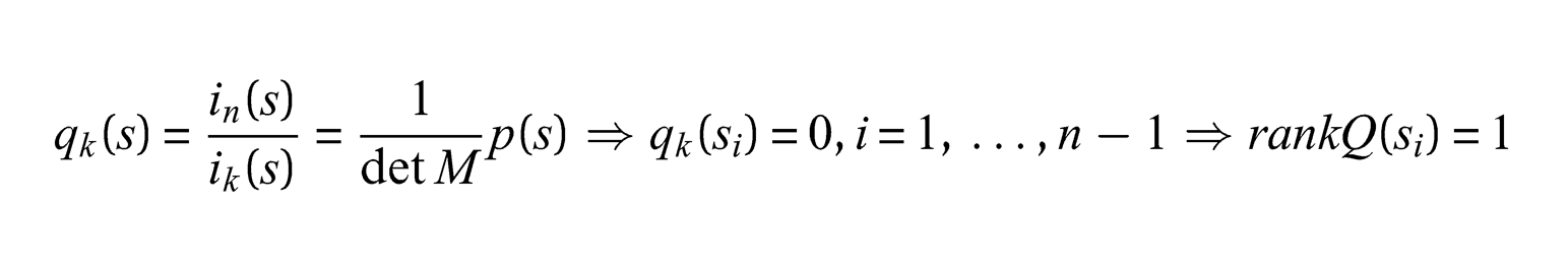
Remark 9.2: The reduced adjoint to the dynamic stiffness is a matrix polynomial satisfying , where is the nth invariant polynomial of (see Appendix A.1.1). It follows that and then , where . Every non-zero column vector in is then an eigenvector to corresponding to the eigenvalue . Now if then, by using the Smith normal form, Theorem A.1.1, one obtains
where
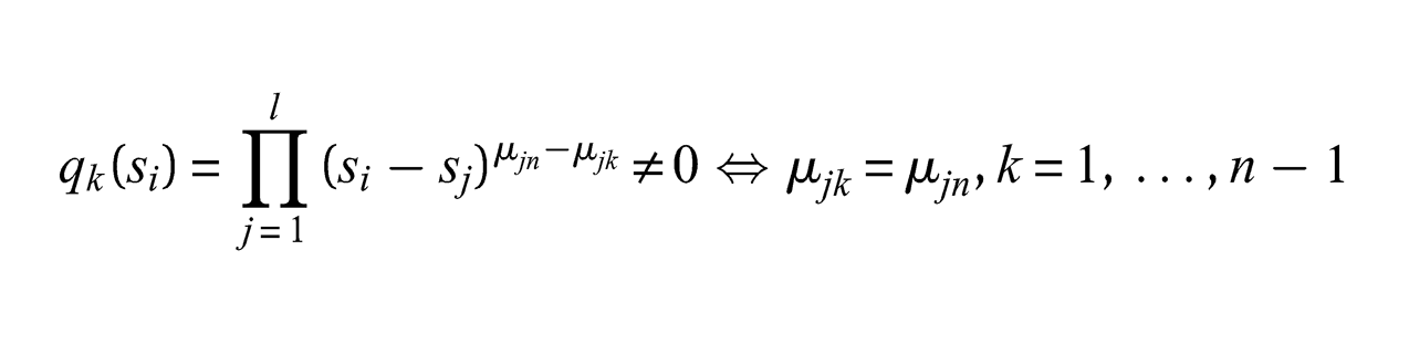
The invariant polynomials are defined in Appendix A.1. Since the quotient is defined for all , the expression for in (72) is valid for all . Then
where
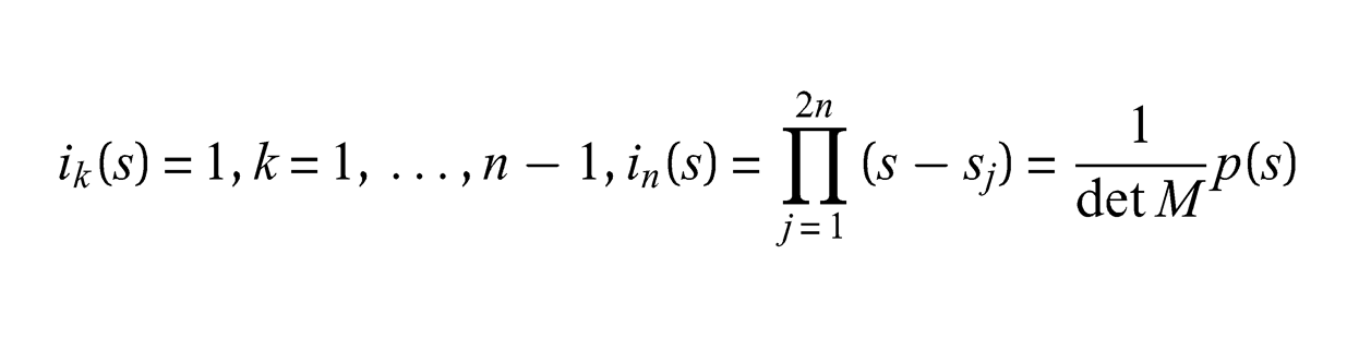
The number of will then be equal to the number of elementary divisors of maximal degree. The rank of is equal to one plus the number of and thus equal to the number of elementary divisors of maximal degree (see Lancaster and Webber [16] (Theorem 1)). Note that if we have simple roots, as in Section 8, then
and
■
Starting from the identity , in the previous remark, we may now formulate the following.
Proposition 9.2 is a zero of the polynomial , with multiplicity , if and only if
Proof: Similar to the proof of Proposition 9.1. □
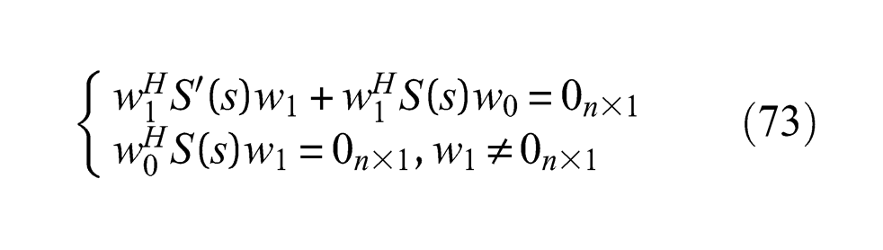
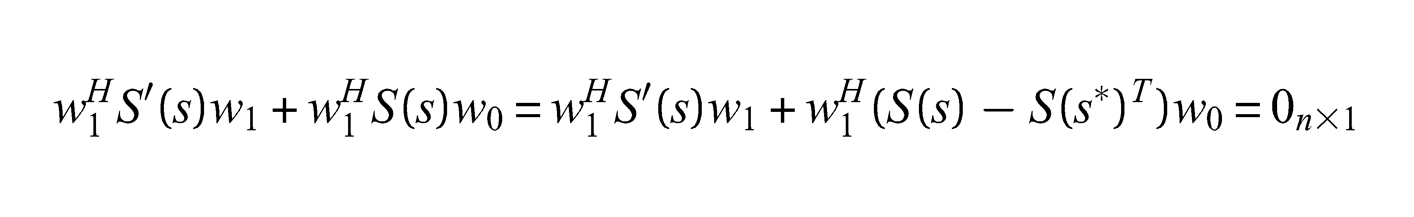
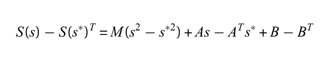
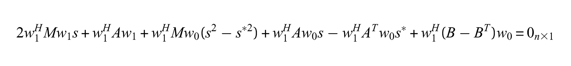
Remark 9.3: Not all generalized eigenvalue problems admit a Jordan chain. For instance, considering the case of a double root, we obtain from (68), by multiplying from the left with and ( means Hermitian transpose, see Appendix A.1), respectively:
By taking the Hermitian transpose of the last expression one obtains and from this and (73)1 one gets
where
and then
Now assume that and , then
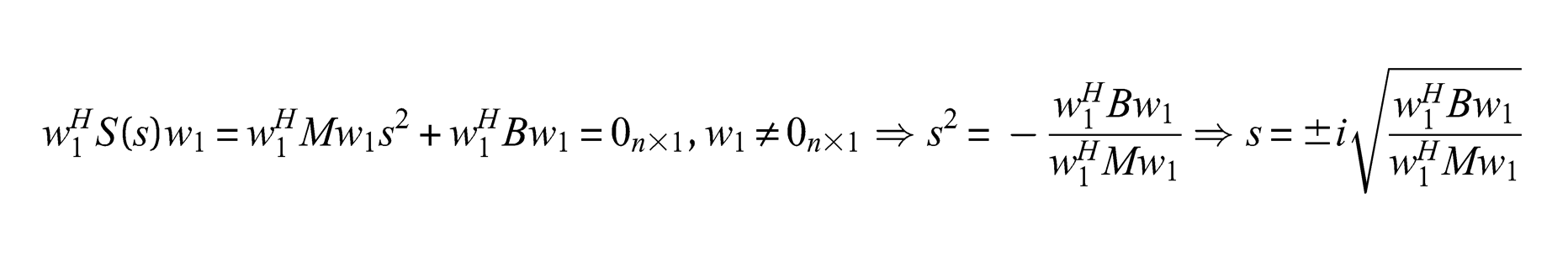
If is positive definite then, according to (68)2:
and from this we may conclude that and then, according to (74), , since and consequently . Thus, a Jordan chain does not exist and Equations (68) are reduced to
For and positive definite, the same argument will work for roots of any multiplicity , which means that and there exists satisfying (70). In this case one may show that there will be linearly independent vectors satisfying equation (75).■
The dynamic stiffness is said to be simple if no eigenvalue is in defect (see Lancaster [10]). In this case we have . This is equivalent to . It follows that if the dynamic stiffness has simple eigenvalues then it is simple. If there is an eigenvalue such that , then is said to be defective. The dynamic stiffness is defective if and only if there is an eigenvalue with an eigenvector such that for all satisfying (see Lancaster [10], (Theorem 4.6)).
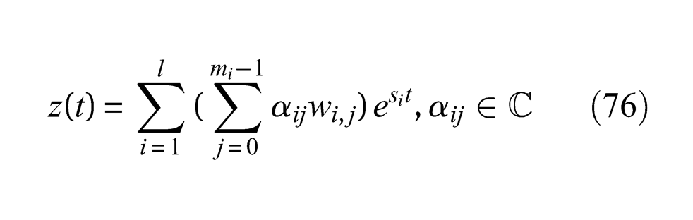
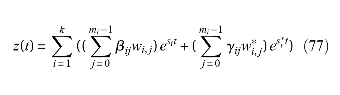
Proposition 9.3 For a system with simple dynamic stiffness let be distinct roots of the characteristic equation with multiplicities and let be a basis for . Then the functions constitute a basis for and a general member of may be written
Proof: Obviously . From Lemma A.1.1(a) it follows that
since are linearly independent. Thus, the functions constitute a basis for . □
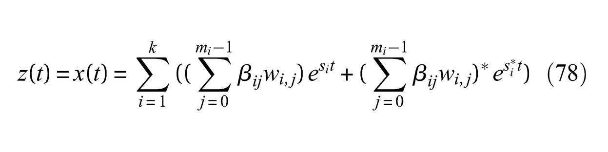
If the roots of the characteristic equation are complex, that is, if , , then (76) may be written
The function (77) is real valued if and only if and in this case
To find the weakest conditions on the coefficient matrices and , resulting in a system with simple dynamical stiffness, is an interesting problem. We have looked into the work of Lancaster and co-workers but not found a definitive solution.
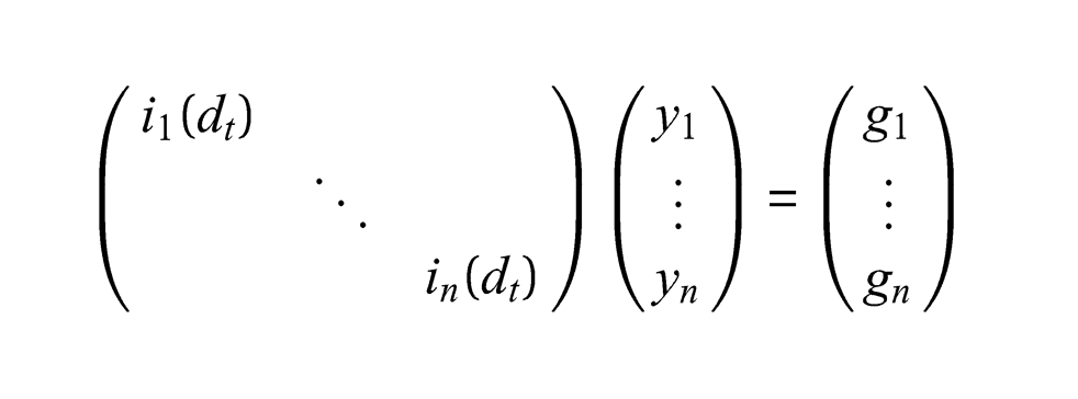
From the previous discussion it may be inferred that the solution of the generalized eigenvalue problem, in the general case, is non-trivial. Methods based on the adjoint and reduce adjoint matrices are accounted for in this paper. An alternative approach to the solution of Equation (43) is based on the Smith canonical form for the dynamic stiffness (see Theorem A.1.1). Based on the Smith form the differential equation (43) may be written , where and then or explicitly
This system uncouples into independent scalar differential equations , and the solution of (43) is then given by (see Gohberg et al. [15]).■
10. The dynamic flexibility
Given a dynamic stiffness with , the corresponding Dynamic flexibility (Admittance) is defined by . Obviously:
For the spectral representation of the Dynamic flexibility one needs the following.
Lemma 10.1 Let be distinct roots of the characteristic equation with multiplicities . For a simple dynamic stiffness there are linearly independent vectors satisfying the orthogonality conditions
where .
Proof: See Lancaster [10] (Theorem 4.5) or [17]. □
Remark 10.1: The vectors may of course be normalized so that . We here prefer the flexibility offered by allowing to be any complex number not equal to zero.■
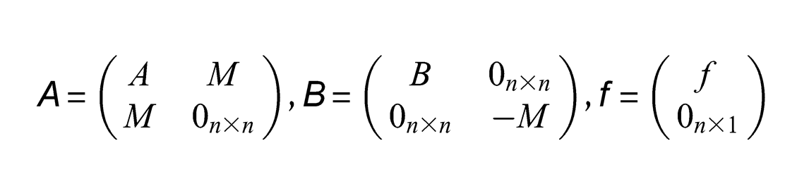
Remark 10.2: By introducing , where , Equation (43) may be written
where
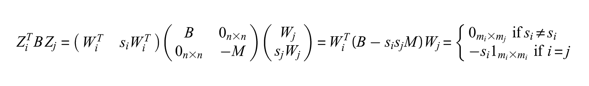
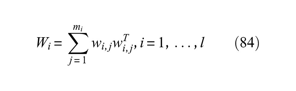
Compare this with the proof of Theorem 6.1. Considering free vibrations we take and , where is a constant vector. Then Equation (81) implies with a solution if and only if . The matrix is called the matrix pencil associated to the dynamic stiffness (see Appendix A.1). If then and . Let be a root of the characteristic equation, that is, , with multiplicity . Consider vectors and the corresponding vectors satisfying , . Note that the vectors are linearly independent if and only if are linearly independent. Now let be a second root with multiplicity and vectors . Introduce the matrices
and
It may be demonstrated that is simple if and only if the associated pencil, , is a simple pencil (see Lancaster [10]). Thus, if is simple then, according to Theorem A.1.2, it is possible to choose vectors and to obtain
Thus
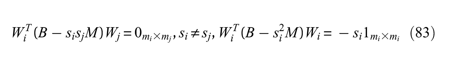
The conditions above may be written
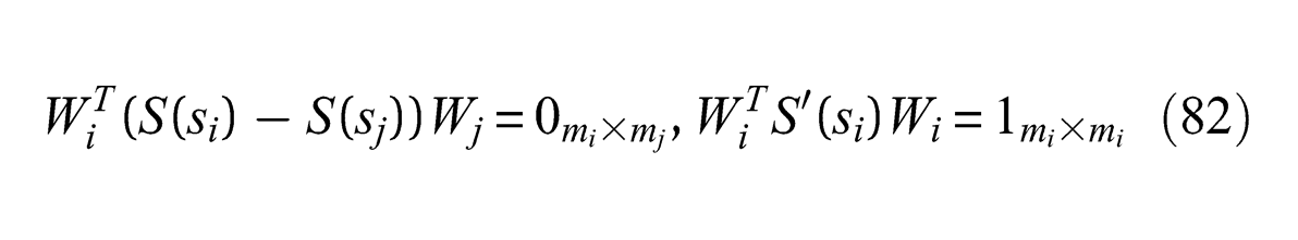
respectively, and (82)2 is equivalent to the orthogonality conditions (80), taking . Furthermore
Thus
The orthogonality conditions (82)1 and (83)1 should be compared with the ones presented in Corollary 8.3 that were obtained for .■
Now, introduce the matrices
The matrix with is called the residue at of the flexibility . The following theorem expresses the dynamic flexibility in terms of modal properties.
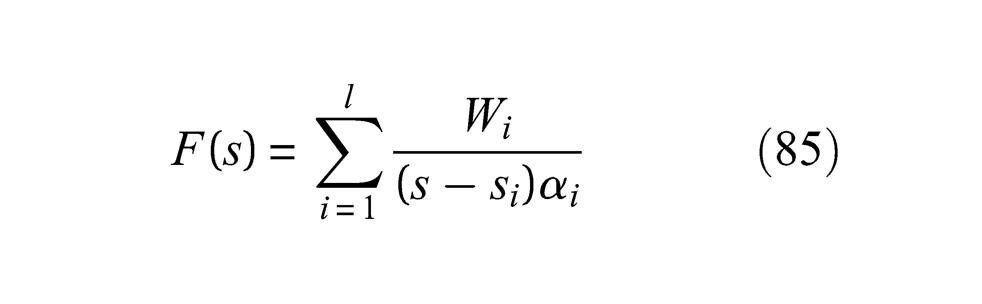
Theorem 10.1 If the dynamic stiffness is simple then
Proof: See Lancaster [10] (Theorem 4.3) and [17]. □
Remark 10.3: If the dynamic stiffness is simple then, according to (85), the flexibility has a pole of order one at .■
Remark 10.4: The dynamic stiffness is simple for many multibody systems encountered in applications. For instance, if and (non-gyroscopic and non-circulatory) and if then is simple.■
The following is a direct consequence of the previous theorem.
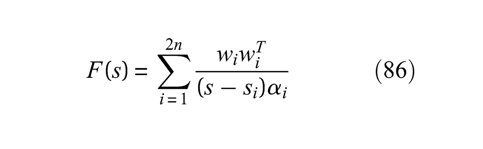
Corollary 10.1 If the dynamic stiffness is simple and in the case of simple roots we have
where .
Proof: In this case . □
The adjoint may be expressed in terms of the modal properties of the dynamic stiffness.
Corollary 10.2 If the dynamic stiffness is simple then
Proof: We have, according to (79) and Theorem 10.1:
□
The dynamic flexibility may be expressed in terms of the adjoint according to the following.
Proposition 10.1 If the dynamic stiffness is simple then
and
Proof: We have
and . Combining these two expressions leads to
and this proves the proposition. □
Corollary 10.3 If the dynamic stiffness is simple, and in the case of simple roots, we have
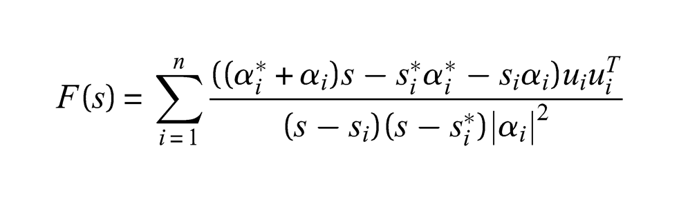
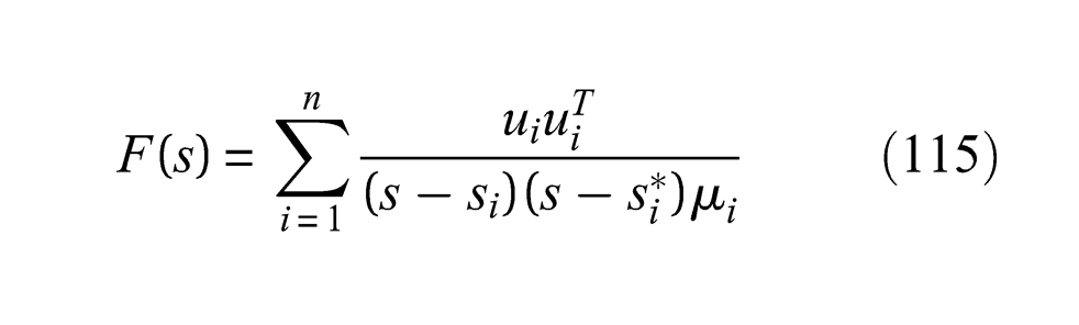
If the dynamic stiffness is not simple then the situation is much more complicated. A representation of the flexibility in terms of modal properties, similar to the one in (85), is not known to the author. However, we have the following general result.
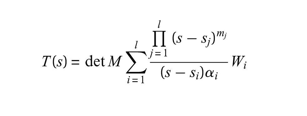
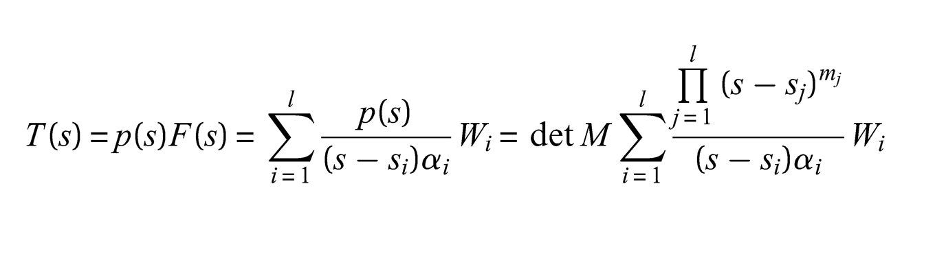
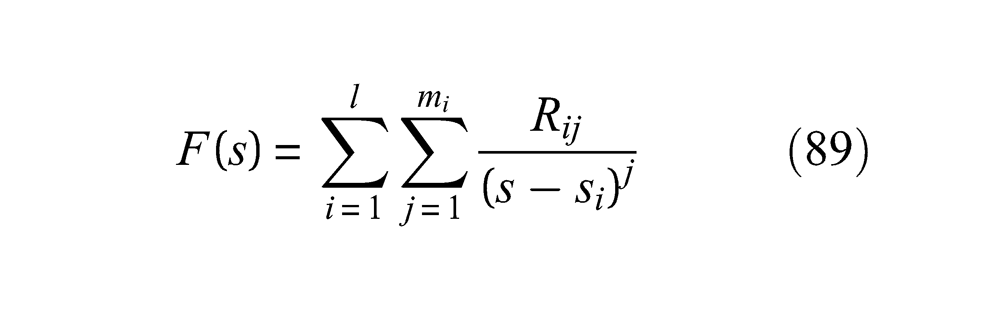
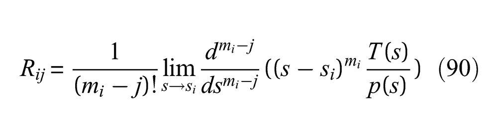
Theorem 10.2 Given a dynamic stiffness . If are roots of the characteristic equation with multiplicities then the flexibility may be written
where the residues are given by
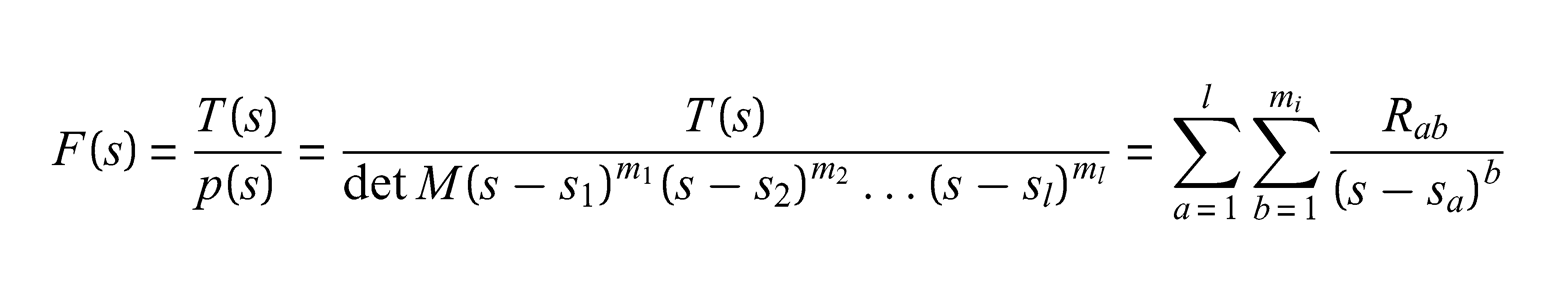
Proof: A partial fraction decomposition of the dynamic flexibility gives
where and are constant matrices. Then
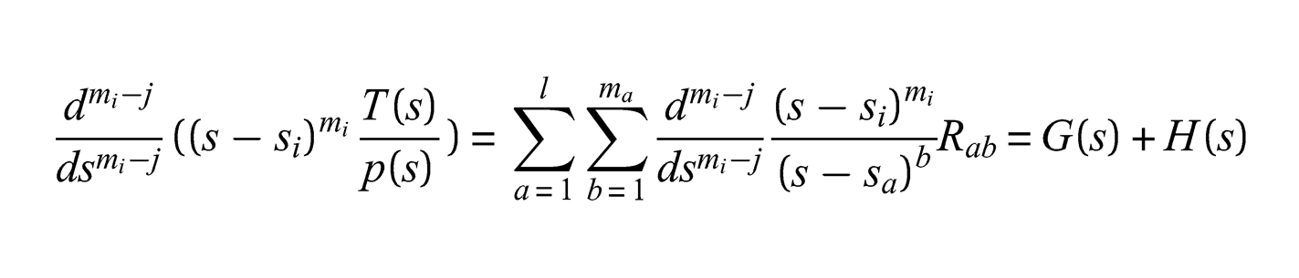
where
Now . Furthermore
Thus and
and this proves the theorem. □
Remark 10.5: For a simple dynamic stiffness one has and . Note that in the case with simple roots we have, according to (90):
which is in agreement with Corollary 10.3.■
Remark 10.6: A general formula relating the residues to the spectral properties (of the generalized eigenvalue problem) of a non-simple dynamic stiffness is not known to the author. This problem is, according to the theorem above, related to the representation of the adjoint in terms of modal properties. The reader is referred to Gohberg et al. [15] where some results related to this problem are presented.■
11. Qualitative properties of damping factor and natural frequency
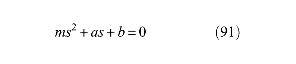
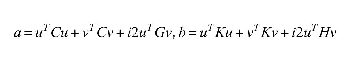
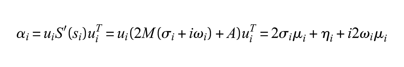
The eigenvalues are determined as roots to the characteristic equation. In this section we will derive some qualitative properties of that follow from physically motivated assumptions on the matrices and . This may be done without explicitly solving the characteristic equation. If , then there exists , such that . By multiplying this equation, from the left, with one obtains the equation
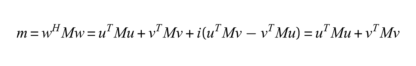
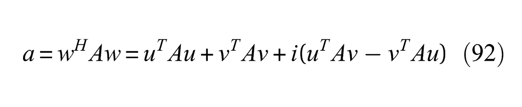
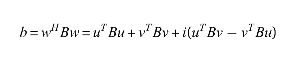
where
We have the decompositions , , where , , and . Inserting this into (92)2,3 results in
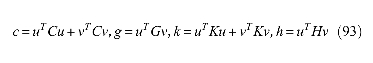
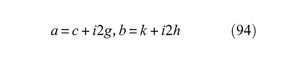
If we introduce the real constants
then
The numerical values of the real constants will of course depend on the actual mode vector . However, some general properties of these constants may be motivated from physical considerations.
Proposition 11.1 If the damping matrix is positive semi-definite then and if is positive definite then . If the stiffness matrix is positive semi-definite then and if is positive definite then .
Proof: This is a direct consequence of (93)1 and (93)3, respectively, and the fact that . □
Lemma 11.1 If the stiffness matrix is positive definite then and consequently .
Proof: Assume that then there exists such that and then , which leads to a contradiction. □
Note that if then and we have where and
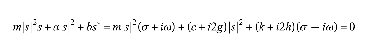
which is equal to the complex conjugation of Equation (91). By multiplying (91) by one obtains
which is equivalent to
Proposition 11.2 If and if and are positive definite then .
Proof: From (95)1 it follows that where, according to Lemma 11.1, . Then, since and :
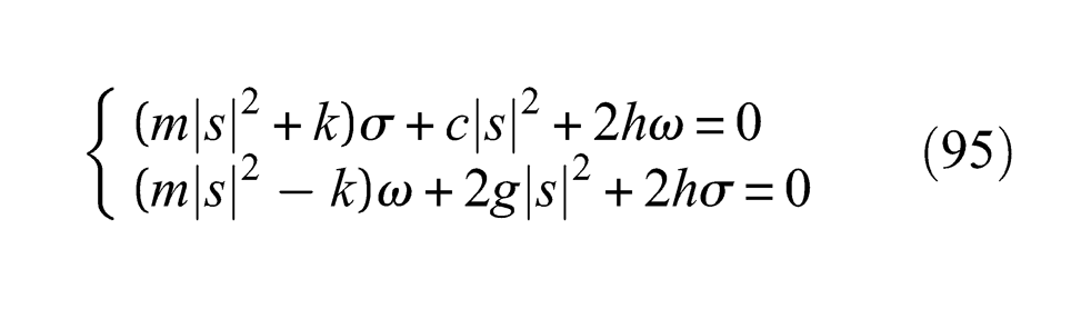
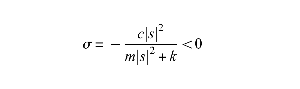
Proposition 11.3 (Gyroscopic conditions) If , and then
Proof: From (95)1 it follows that and then from (95)2
and this proves the proposition. □
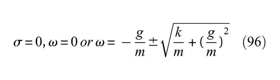
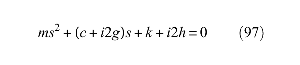
Remark 11.1: Note that if is positive definite then, according to Lemma 11.1, in (96) is excluded.■
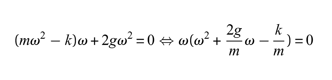
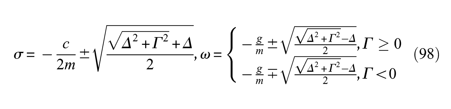
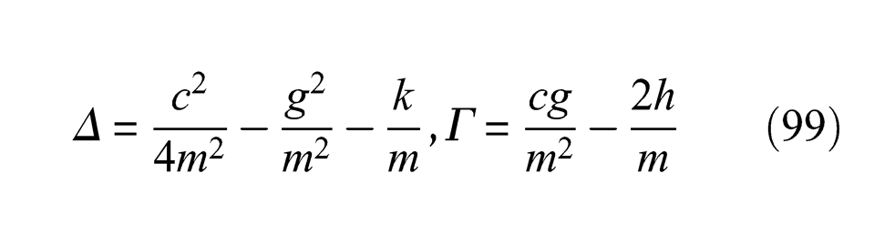
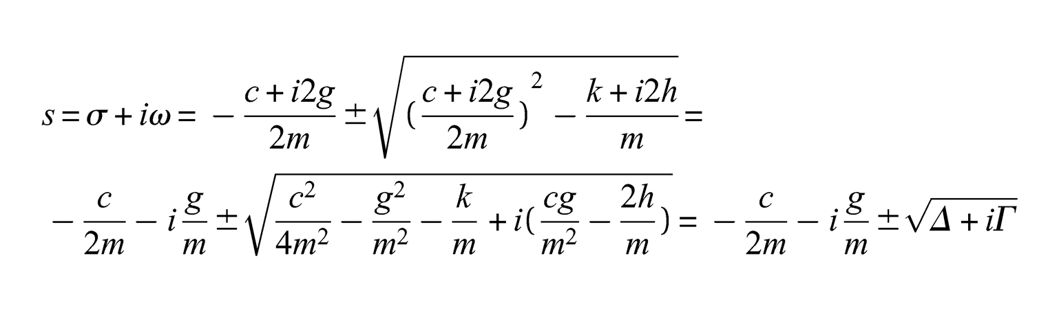
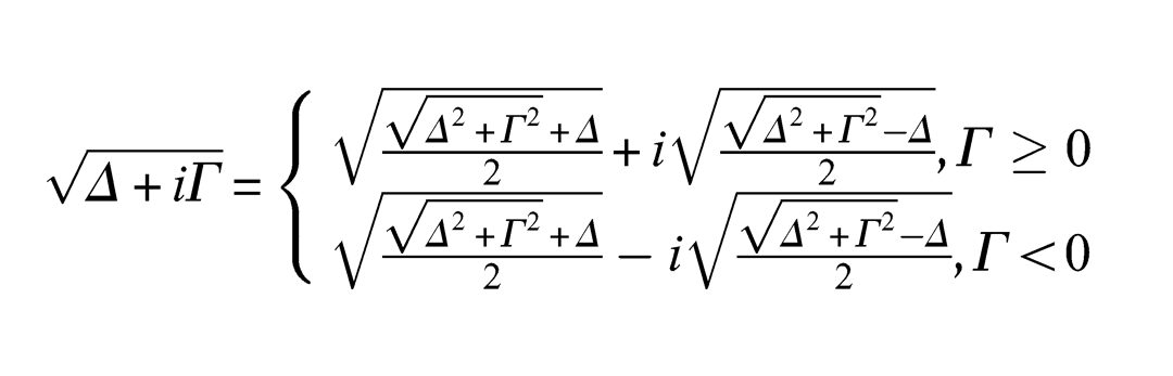
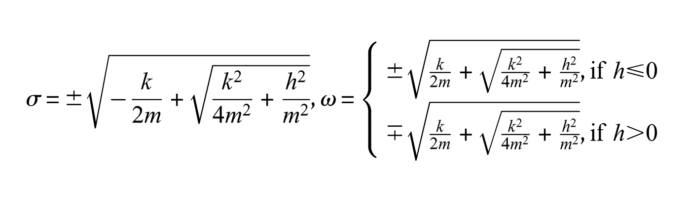
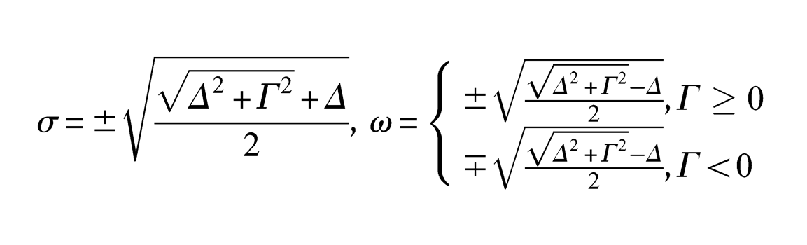
Proposition 11.4Equation (97) has the solutions where
and
Proof: We have
where
and this proves the proposition. □
Remark 11.2: Note that we cannot make any definitive decision on the signs in (98). These will depend on the mode shape vector .■
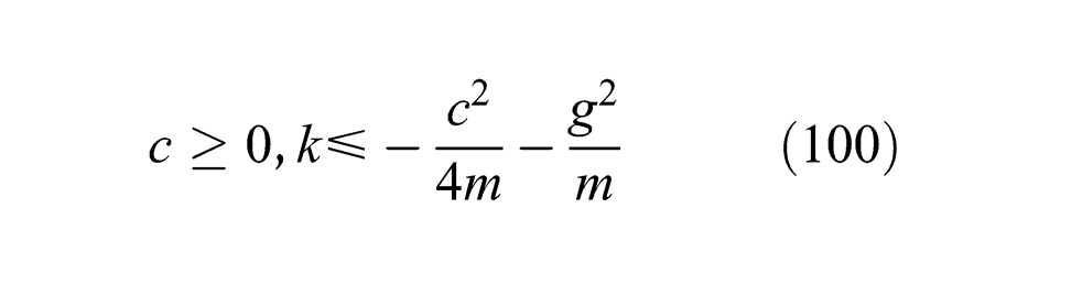
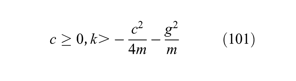
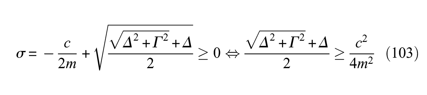
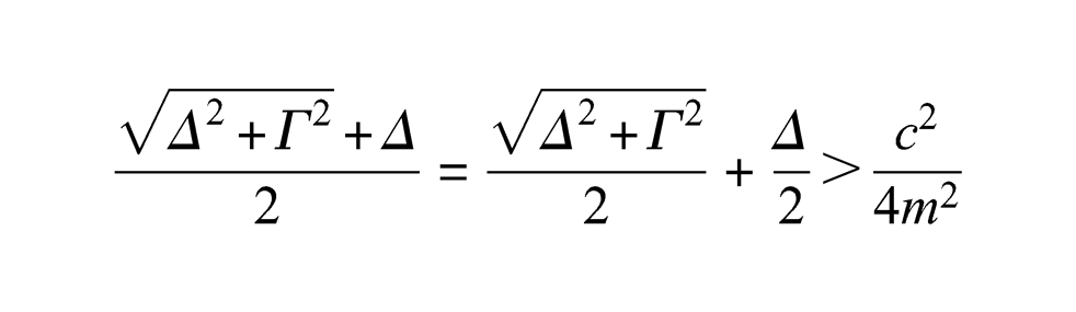
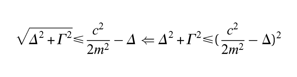
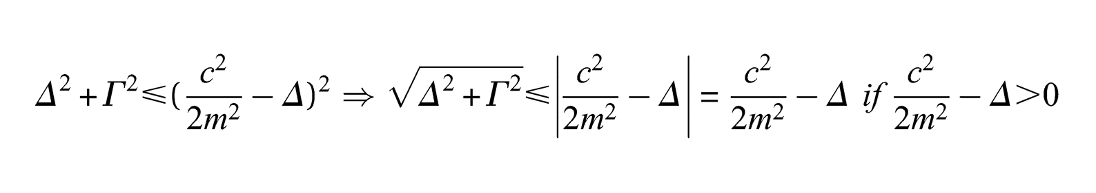
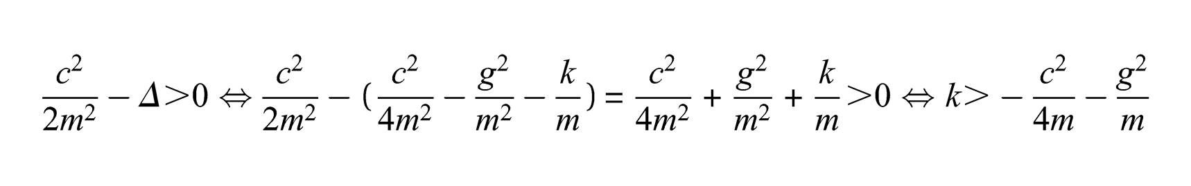
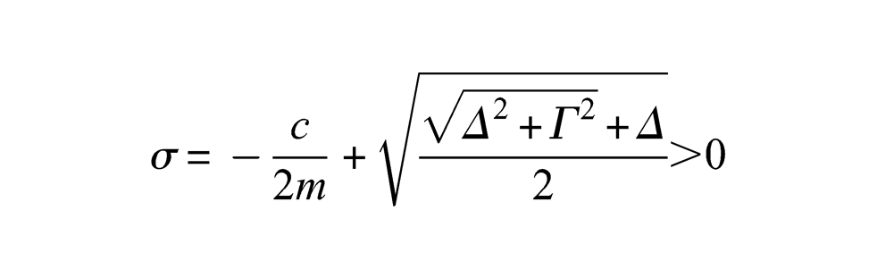
Proposition 11.5 (Stability) (a) If
then . (b) If
then if and only if
and if and only if .
(c) If then .
Proof: (a) If then we have the following equivalence:
From (99)1 and (100)1 one obtains
and then
and consequently . (b) We have the implications
It remains to show the implication
But
This condition being equivalent to
(c) If then
This proves the proposition. □
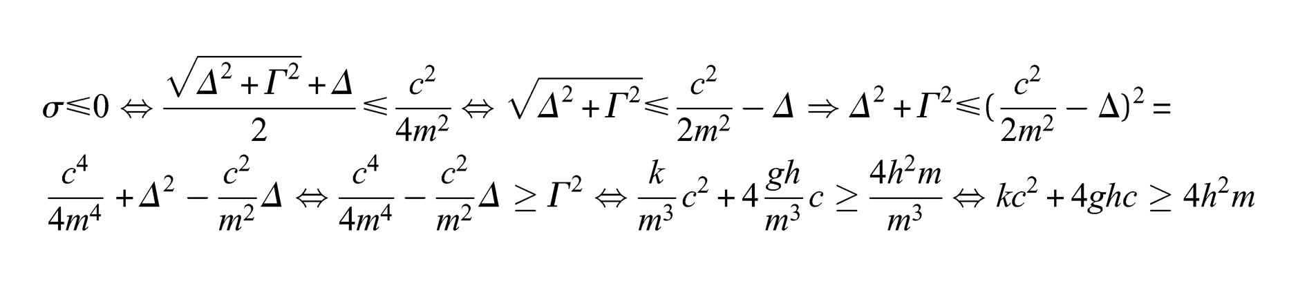
Remark 11.3: (Instability) From the previous proof it follows that if then
■
Remark 11.4: It follows from the previous proposition that if , and then . Thus a gyroscopic system may be destabilized by introducing circulatory forces.■
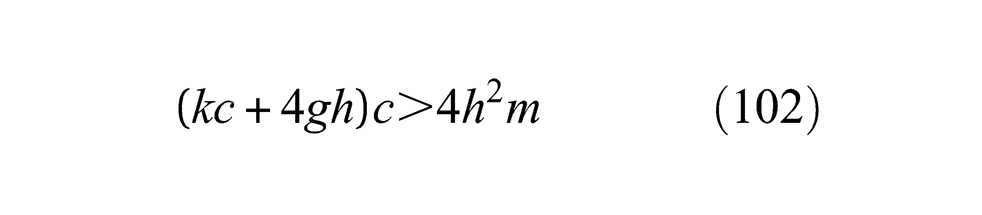
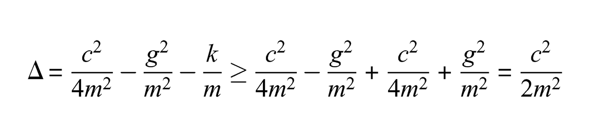
Corollary 11.1 If inequality (102) is satisfied, (non-circulatory conditions) and
(a) then if and only if ;
(b) then .
Proof: (a) From (102) it follows that if then . (b) If and then inequality (102) leads to a contradiction. Thus . □
Remark 11.5: Note that (101) is valid if , and . This suggests that the damping term may have a destabilizing influence on a system where the potential energy has a maximum at . A closer analysis will confirm this. See Example 11.1 below and Krechetnikov and Marsden [18]■
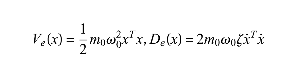
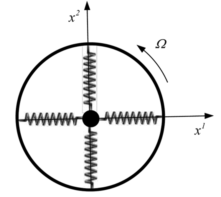
Example 11.1: Consider a particle with mass connected by linear elastic (massless) springs to a circular ring that is rotating with a given angular velocity (see Figure 3). Let denote Cartesian configuration coordinates of the particle relative to the ring and put . The elastic energy and the dissipation function of the system are assumed to be given by
where , and are positive constants.
Two-dimensional multibody system.
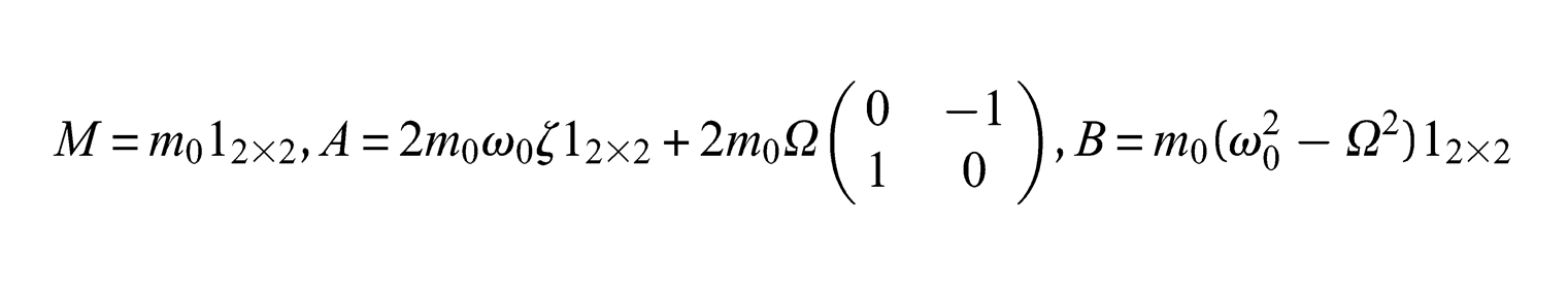
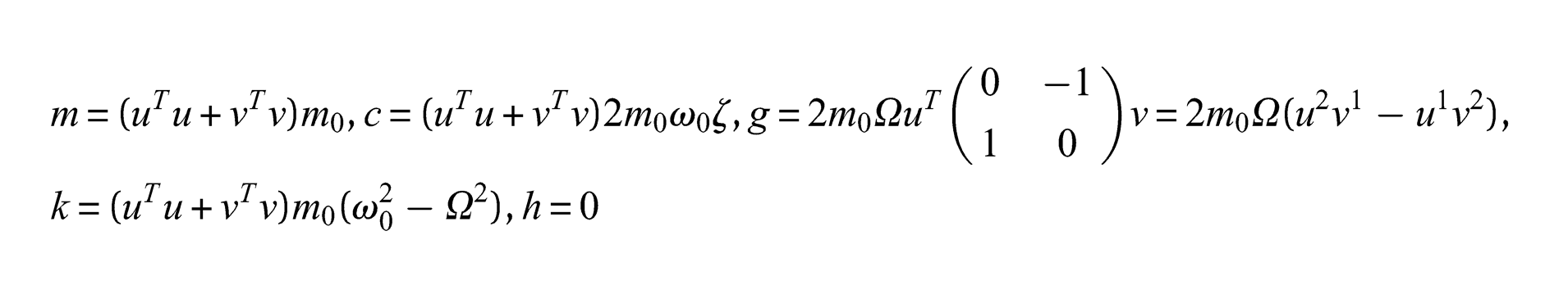
The dynamic stiffness matrix of the system where
Thus , , and and consequently
The condition (101)2 may be written
Without loss of generality we may choose . Thus
which is satisfied if
since . The left inequality follows from , where we have used the fact that . The system is thus stable if and only if .■
The following corollaries are direct consequences of Proposition 11.4.
Corollary 11.2 (Non-gyroscopic and non-circulatory conditions) If , then
(a) if : , (over-damped)
(b) if : , (under-damped)
Corollary 11.3 (Gyroscopic conditions) If , then
Proof: If , then and consequently, according to (98):
However, and then (104) follows from (105). □
Remark 11.6: Properties of overdamped and gyroscopic systems are discussed by Duffin [19], Rogers [20], Inman [21], Brackwell and Lancaster [22] and Lancaster et al. [23].■
Corollary 11.4 (Non-damped and non-gyroscopic conditions) If , then
Proof: If , then, according to (98):
where , and this proves the corollary. □
Remark 11.7: Let , and assume that and are positive definite. The system is then said to be over-damped if for all . Let , , and assume that is non-negative definite. The system is then said to be gyroscopic. It may be shown that if the system is over-damped or gyroscopic then the dynamic stiffness is simple (see Lancaster [10]).■
12. Forced vibrations
Consider the non-homogeneous linearized equation of motion
where the external force is a prescribe function. The general solution, the response, is given by , where and is any function satisfying .
Now let be a solution to the inhomogeneous characteristic differential equation . If is sufficiently differentiable then put . The function is then a solution to (106) since
Assume that the external force is harmonic, where is a constant vector and . We may complexify the problem by taking , where and consider the equation
If is a solution to (107) for then is a solution to (106) with . Assume that is a solution to (107), where is a time-independent vector to be determined. Then
if . Using (89) one obtains
and then
and, consequently, in the case with harmonic external force then
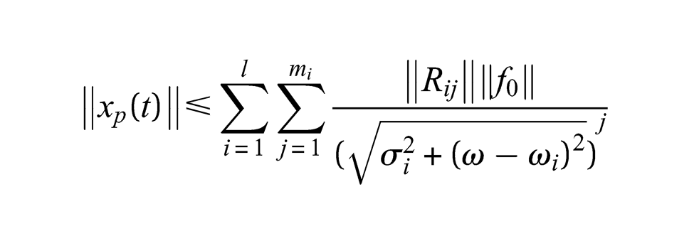
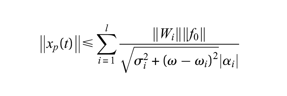
We have the following estimate:
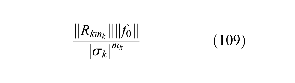
If (resonance) and then the term with and on the right-hand side of the inequality reads
and if and is large then the denominator is a small number rendering the quotient large if the nominator is not too small. Thus, the amplitude of resonances in systems with multiple eigenvalues may become very large.
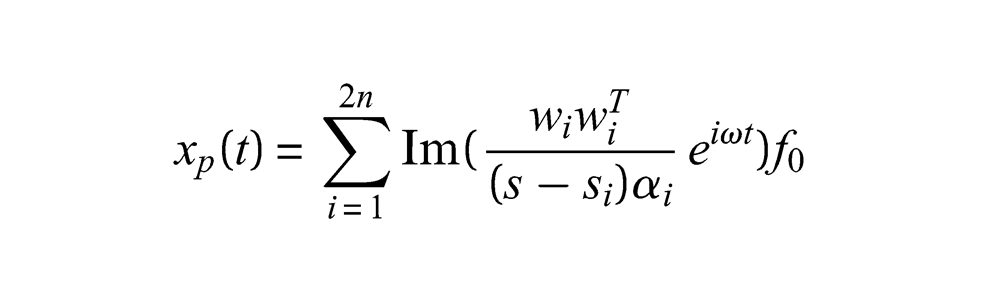
If the dynamic stiffness is simple then the dynamic flexibility is given in (85) and
In the case of a harmonic external force we then obtain
We have the following estimate:
where . If (resonance) and then the term with on the right-hand side of the inequality reads
By comparing this expression with (109) it is clear that if the dynamic stiffness is simple then the resonance is not as prominent as it may be in the general case.
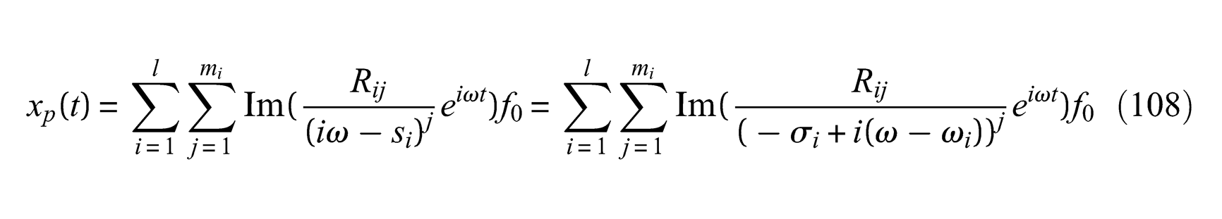
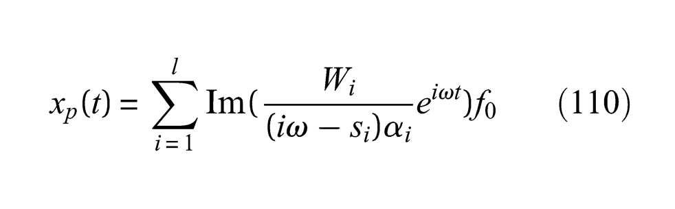
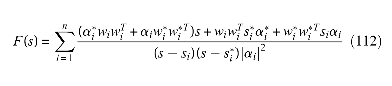
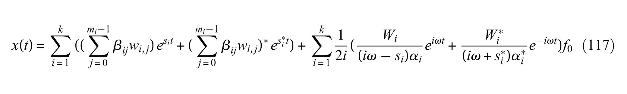
If the roots of the characteristic equation are simple then the dynamic flexibility is given by (86) and for a harmonic external force we then obtain the response
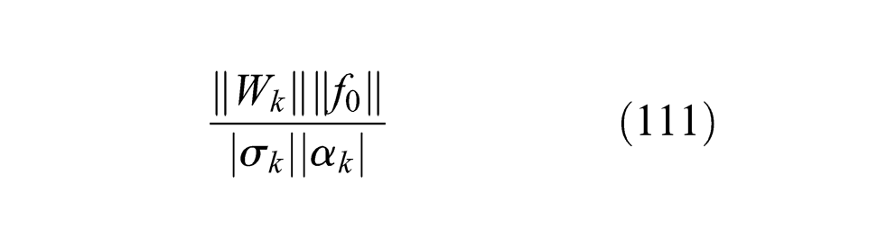
From the engineering point of view resonances are important, since they may give rise to a magnification of the response amplitude. In this perspective it is clear that multiple roots may form a greater risk of high amplitudes than simple roots, since the amplitude in (111) compares with
in the case of simple roots.
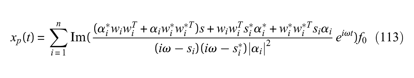
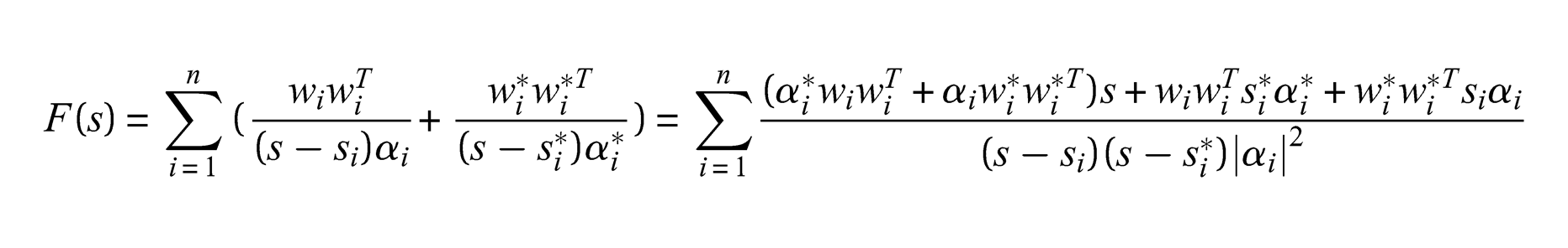
Proposition 12.1 If the roots of the characteristic equation are simple and complex, that is if , then
and if the external force is harmonic then
Proof: From (86) it follows that
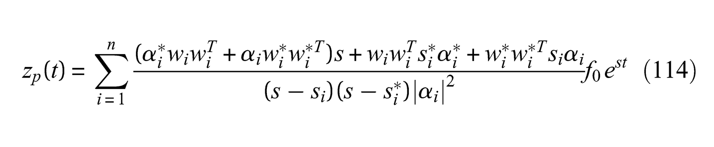
The complexified solution is given by
and the real solution (113) is obtained by putting into (114) and then selecting the imaginary part. □
Remark 12.1: In the case of real modes and then, according to (112):
where
and , . If we assume that , which is the case for non-gyroscopic and non-circulatory systems, then , , and . Consequently
■
According to Equation (46) the characteristic polynomial may be written , where all are distinct complex numbers and . If all roots are complex then and we may write
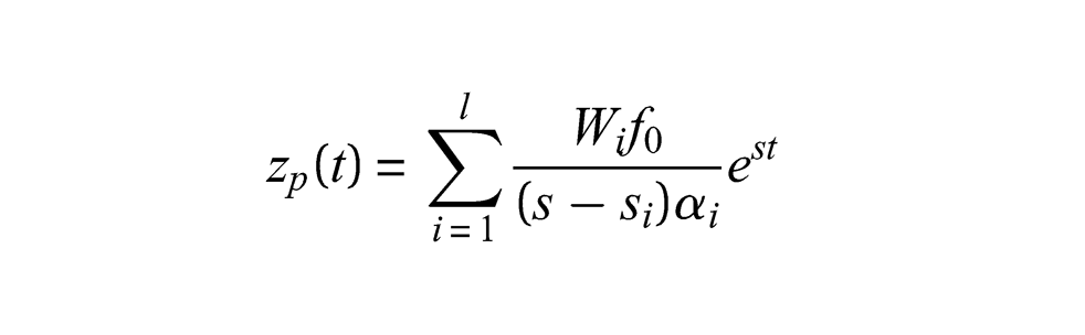
where. We end this section with the following theorem.
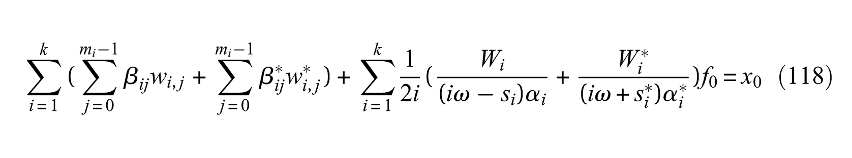
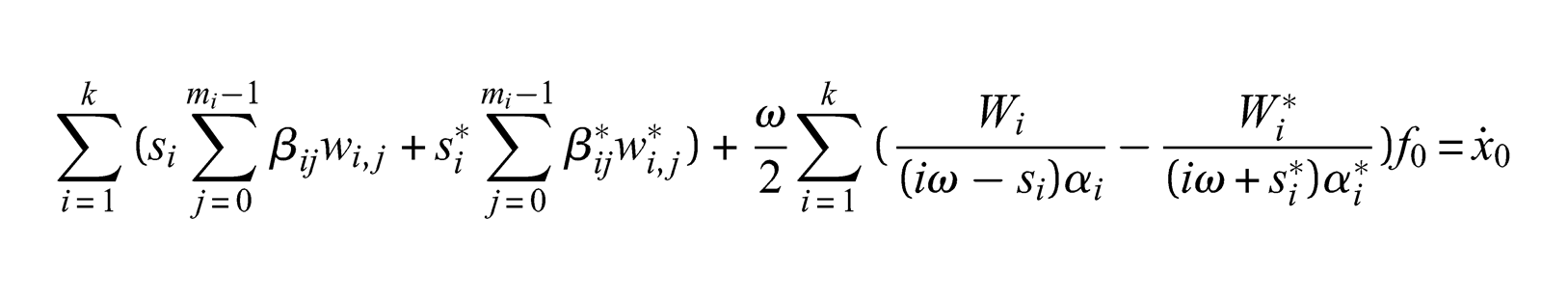
Theorem 12.1 If the roots of the characteristic equation are complex, that is if , , () are distinct roots with multiplicities , then for a system with simple dynamic stiffness the solution to the initial value problem
is given by
where the complex constants are uniquely determined by
Proof: This is a direct consequence of (78) and (110). □
13. Concluding remarks
In this paper the linearized equations of motion in multibody dynamics have been derived. The multibody is assumed to consist of rigid parts as well as parts consisting of visco-elastic material. Parts are connected by ideal joints and it is assumed that an equilibrium configuration for the multibody system exists. The analysis of the linearized equations of motion is based on a consequent use of the differential operator related to the dynamic stiffness of the system and its adjoint. This approach seems to be novel, at least in the engineering literature. It has the advantage of retaining the original differential equation with its close connection to the basic principles of mechanics. The solution of the linearized equations involves the solution of a (generalized) eigenvalue problem involving a Jordan chain. It is demonstrated how the solution can be obtained from the adjoint of the stiffness matrix. Some seemingly open problems have been identified:
- to find the weakest conditions on the coefficient matrices and , resulting in a system with simple dynamical stiffness;
- a general formula relating the residues to the spectral properties (the generalized eigenvalue problem) of a general (non-simple) dynamic stiffness.
A non-trivial extension of the multibody model presented in this paper might involve the incorporation of friction and visco-elastic bushing elements at joints. This will be addressed in a forthcoming paper.
Footnotes
Appendix
Funding
This research received no specific grant from any funding agency in the public, commercial or not-for-profit sectors.
Conflict of interest
None declared.
References
1.
Lord Rayleigh. The theory of sound (two volumes), New York: Dover Publications, 1945.
2.
HughesTJR. The finite element method. Linear static and dynamic finite element analysis. Englewood Cliffs, NJ: Prentice Hall, Inc., 1987.
3.
GéradinMRixenD. Mechanical vibrations. Theory and applications to structural dynamics. Chichester: John Wiley & Sons, 1997.
4.
LidströmP. On the equations of motion in multibody dynamics. Math Mech Solid2012; 17: 165–205.
5.
BirkhoffGRotaG-C. Ordinary differential equations. 3rd ed.New York: John Wiley and Sons, 1978.
6.
ArnoldVI. Ordinary differential equations. Cambridge MA: The MIT Press, 1973.
7.
FossKA. Co-ordinates which uncouple the equations of motion of damped linear dynamic systems. J Appl Mech1958; 25: 361–364.
8.
CaugheyTK. Classical normal modes in damped linear structures. J Appl Mech1960; 27: 269–271.
9.
CaugheyTKO’KellyMEJ. Classical normal modes in damped linear dynamic systems. J Appl Mech1965; 32: 583–588.
10.
LancasterP. Lambda-matrices and vibrating systems. Oxford: Pergamon Press Inc., 1966.
11.
LidströmP. On the relative rotation of rigid parts and the visco-elastic torsion bushing element. Math Mech Solid2013; 18: 788–802.
12.
LidströmP. On the equations of motion in constrained multibody dynamics. Math Mech Solid2012; 17: 209–242.
13.
CloughRWPenzienJ. Dynamics of structures. Düsseldorf: McGraw-Hill, 1975.
14.
WuLGreifR. The eigenproblem for damped linear vibrating systems with multiple eigenvalues. J Sound Vib1989; 131: 197–214.
15.
GohbergILancasterPRodmanL. Matrix polynomials. New York, London: Academic Press, 1982.
16.
LancasterPWebberPN. Jordan chains for lambda matrices. Lin Algebra Appl1968; 1: 563–569.
17.
LancasterP. Inversion of lambda-matrices and application to the theory of linear vibrations. Arch Ration Mech Anal1960; 6: 105–114.
18.
KrechetnikovRMarsdenJE. Dissipation-induced instabilities in finite dimensions. Rev Mod Phys2007; 79: 519–553.
19.
DuffinRJ. A minimax theory for overdamped networks. J Ration Mech Anal1955; 4: 221–233.
20.
RogersEH. A minimax theory for overdamped systems. Arch Ration Mech Anal1964; 16: 89–96.
21.
InmanDJ. A sufficient condition for the stability of conservative gyroscopic systems. J Appl Mech1988; 55: 895–898.