On the notion of embedded homogeneity of thin structures

Abstract

A thin-walled structure is homogeneously embeddable if it can be obtained by carving it out of a homogeneous material block or, in other words, if it is materially defect-free. Explicit analytic and geometric conditions for the embedded homogeneity of plane linearly elastic beams are derived and discussed. In the geometric setting, a prominent role is played by the properties of the hodograph of uniaxial material tensor fields defined on the beam axis.

Keywords

Inhomogeneity elasticity hodograph differential geometry generalized Serret–Frenet formulas osculating sphere

1. Introduction

By definition, the theories of beams and shells are formulated upon curves and surfaces embedded in a three-dimensional Euclidean space. In the most widespread version of shell theory, for example, the strain measures express the change brought about by the deformation on the first and second fundamental forms of the surface, while the internal static quantities consist of tensors of membrane forces and moments. Correspondingly, an elastic constitutive response is expressed in terms of functions relating these static quantities with the strain measures. Clearly, when viewed as an independent theory of an embedded elastic surface, questions of material symmetry, uniformity and homogeneity can be handled intrinsically, within the compass of the theory [1, 2, 3, 4]. Consider, however, a shell that has been cut from a perfectly homogeneous block. If, using the three-dimensional constitutive equations of this block, a relation between the above mentioned strain measures and the internal static quantities is obtained by a standard integration of the stress tensor over the thickness of the shell, two shell points may not turn out to be shell-wise materially isomorphic due to a lack of isotropy of the underlying material or, even when this material is isotropic, a possible mismatch between the curvature tensors. Placed under the microscope of a material scientist, on the other hand, no dislocations or other material imperfections will be detected.

These intuitive considerations lead to the following question: Given a constitutive law of an elastic shell in terms of forces, moments, membrane stretches and curvature changes, is it possible to ascertain the homogeneity or otherwise of the underlying material out of which the actual physical shell is made? We call this the embedded homogeneity problem. It has been already introduced, but not developed, in [2].

The problem will be first formulated in a purely analytic fashion. As one is wont to do in dislocation theories, however, a geometric formulation and interpretation, with their typical elegance and intuitive appeal, will also be provided. To facilitate the exposition and to emphasize the salient aspects of the theory, we will confine ourselves in this paper to linear elasticity and to the simplest of structures, viz. plane beams, leaving the treatment of spatial beams, membranes and shells for a forthcoming exposition.

2. Analytic formulation

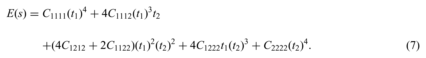
Our point of departure is a two-dimensional planar sheet made of a homogeneous and linearly elastic material in a stress-free reference configuration. In a Cartesian coordinate system $(x_{1}, x_{2})$ , the constitutive response is, therefore, completely characterized by a fourth-order constant tensor $ℂ$ of components $C_{α β μ σ}$ with the symmetries

C_{α β μ σ} = C_{β α μ σ} = C_{μ σ α β} .

(1)

Let now a curved beam be cut from this sheet with a middle axis $Γ$ described by the differentiable functions

x_{α} = x_{α} (s) α = 1, 2,

(2)

assumed to represent an embedded submanifold (so that, in particular, the curve does not self-intersect). The parameter $s$ may be assumed to measure length along $Γ$ . For simplicity, we assume the normal thickness $h$ of the beam to be constant. In the Euler–Bernoulli formulation, normals to the beam axis are assumed to remain normal and unstretched throughout the deformation process. Under these conditions, the strain field in the beam is completely defined by means of two scalar fields $γ (s)$ and $ρ (s)$ , measuring, respectively, the axial strain and the curvature change at a point $s$ of the beam axis. A straightforward integration of the two-dimensional stress field yields the constitutive equations of the beam in terms of the two formulas

N (s) = E (s) f (h, κ, γ, ρ),

(3)

and

M (s) = E (s) g (h, κ, γ, ρ) .

(4)

In these equations, $N$ and $M$ are, respectively, the axial force and bending moment, $κ = κ (s)$ is the curvature of the axis before deformation, and $E (s)$ is a modulus of elasticity in the direction of the beam axis. It is worth pointing out that the functions $f$ and $g$ are universal, that is, independent of the elastic properties. Moreover, the elastic coefficient $E (s)$ is obtained from the elastic constants of the sheet by means of the formula

E (s) = ℂ (t, t, t, t) = C_{α β μ σ} t_{α} t_{β} t_{μ} t_{σ},

(5)

where the summation convention in the range $1, 2$ is enforced and where $t = t (s)$ is the unit vector tangent to the beam axis. Its Cartesian components are

t_{α} = \frac{d x_{α}}{ds} = {x'}_{α}, (α = 1, 2),

(6)

measuring, respectively, the cosine and the sine of the angle between the tangent line and the $x_{1}$ axis. More explicitly,

\begin{matrix} E (s) = C_{1111} {(t_{1})}^{4} + 4 C_{1112} {(t_{1})}^{3} t_{2} \\ + (4 C_{1212} + 2 C_{1122}) {(t_{1})}^{2} {(t_{2})}^{2} + 4 C_{1222} t_{1} {(t_{2})}^{3} + C_{2222} {(t_{2})}^{4} . \end{matrix}

(7)

We conclude that if an elastic beam has been carved out from a homogeneous sheet its constitutive laws must necessarily have the forms (3) and (4) and, moreover, the coefficient $E (s)$ must be in the linear hull of the five linearly independent functions ${(t_{1})}^{4}, {(t_{1})}^{3} t_{2}, {(t_{1})}^{2} {(t_{2})}^{2}, t_{1} {(t_{2})}^{3}, {(t_{2})}^{4}$ .

Vice versa, assume that beam constitutive laws of the forms (3) and (4) have been specified in the definition of a (stress-free) beam as a self-sufficient structure, without any reference to an underlying material from which it might have been cut. The beam is, clearly, a two-dimensional entity, albeit represented in one dimension. Is this two-dimensional (“real”) beam homogeneous in the sense, for example, that it contains no defects? More precisely, does there exist a smooth extension of the field $E (s)$ to a constant tensor field $ℂ$ in an open neighbourhood of the beam? In light of the previous analysis, we must conclude that such a (not necessarily unique) extension exists if the function $E (s)$ lies in the linear hull of the five basis functions just enumerated. If $E (s)$ is analytic, this condition is equivalent to the vanishing of the Wronskian determinant associated with the six functions at play. (Note that, in view of the trigonometric identity ${(t_{1})}^{4} + 2 {(t_{1})}^{2} {(t_{2})}^{2} + {(t_{2})}^{4} = 1$ , the Wronskian can be somewhat simplified.)

As intuitively predictable, if the function $E (s)$ happens to be a constant $E$ , then an isotropic homogeneous extension always exists. Indeed, setting $C_{1111} = C_{2222} = E, C_{1112} = C_{1222} = 0, C_{1122} = ν E, C_{1212} = E (1 - ν) / 2$ , where $ν \neq 1$ is an arbitrary constant, equation (7) is satisfied identically. On the other hand, unless carefully calibrated, an arbitrarily specified modulus $E (s)$ will result in non-homogeneity. In a circular beam of radius $R$ , for instance, the specification

E (s) = 2 - \cos^{4} (s / R),

(8)

gives rise to a defect-free beam, whereas a linear dependence in $s$ does not!

3. The geometric picture

3.1. A preliminary exercise

When viewed in Cartesian components, symmetric tensors can be regarded as vectors in higher dimensional Euclidean spaces. If done appropriately, the correspondence between tensors and vectors can be made to preserve the inner product in a precise sense. Postponing for a moment the details of these transformations, the operation represented by equation ((5)) can be rigorously regarded as a projection of a vector of appropriate dimension on a given direction. These observations are heuristically sufficient to consider and solve the following elementary problem of two-dimensional Euclidean geometry.

Problem 1. Given a curve $Γ$ in $ℝ^{2}$ and a tangent vector field $w$ over $Γ$ , determine whether there exists a constant vector field $V$ over $ℝ^{2}$ such that $w$ is the projection of $V$ on $Γ$ .

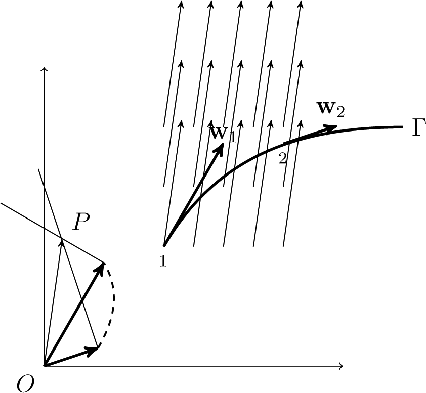
Solution: Figure 1 illustrates the statement of the problem. Let 1 and 2 be two distinct points on the curve and let $w_{1}$ and $w_{2}$ denote the respective tangent vectors. Translating these two vectors to the origin $O$ and drawing the respective perpendiculars at the vector tips, it is clear that their intersection $P$ defines the unique vector $\overset{\leftarrow}{OP}$ whose projection on the curve tangents at 1 and 2 delivers the vectors $w_{1}$ and $w_{2}$ , respectively. Since this construction can be carried out for any pair of points on $Γ$ , we conclude that a constant vector field with the desired property exists if, and only if, all the perpendiculars meet at one and the same point $P$ . The curve obtained by translating each vector $w$ to a common origin $O$ is known as the hodograph of the given vector field. We thus conclude that for the problem to have a solution the hodograph has to have the property that there exists a fixed point $P$ such that the lines joining each point of the hodograph with $O$ and with $P$ are mutually perpendicular. From elementary geometry, we know that this property is satisfied by a circular arc and that $OP$ is a diameter. The hodograph is schematically shown as a dashed curve in the figure.

Figure 1.

The projection problem.

This result can be generalized to a curve and its hodograph in an arbitrary number of dimensions, as stated in the following lemma.

Lemma 3.1. A nowhere vanishing tangent vector field defined on a differentiable curve in $ℝ^{n}$ is the projection of a constant vector field if, and only if, the corresponding hodograph lies on a hyper-sphere containing the origin.

Proof. If $r$ denotes the position vector in $ℝ^{n}$ , the equation of the hyper-sphere with centre at $a$ and radius $R$ is

(r - a) \cdot (r - a) = R^{2},

(9)

where $\cdot$ denotes the ordinary inner product in $ℝ^{n}$ . If the hyper-sphere contains the origin, we must have $R^{2} = a \cdot a$ . Let $Γ$ be a curve with (length) parameter $s$ and let $t = t (s)$ be its unit tangent field. Then, a nowhere vanishing tangent vector field $w$ is uniquely represented as

w = w (s) = E (s) t,

(10)

where $E (s)$ is a nowhere vanishing scalar field on $Γ$ . The hodograph is, therefore, the curve with equation

r (s) = E (s) t .

(11)

If this hodograph lies on a hyper-sphere containing the origin, there exists a fixed vector $a$ such that

(E (s) t - a) \cdot (E (s) t - a) = a \cdot a,

(12)

which implies that

2 a \cdot t (s) = E (s) .

(13)

Conversely, given $E (s)$ (whether or not it vanishes at some points), if equation (13) is satisfied for some fixed $a$ , the steps can be reversed to show that the hodograph lies on a hyper-sphere containing the origin. □

Note 1. If a given tangent vector field is of constant length $E$ , the hodograph further lies on a hyper-sphere with centre at the origin and radius $E$ . In $ℝ^{2}$ the intersection of two circumferences consists of just two points, but in higher dimensions this intersection is a sphere of lower dimension so that one can construct vector fields of constant length on nontrivial curves enjoying the properties of the lemma.

3.2. The space $S_{4}^{2}$ and its linear isometry with $ℝ^{6}$

Let $Lin$ be the set of all second order tensors on an $n$ -dimensional inner product space $V$ . We define [5] the tensor product $A \otimes B$ between $A$ and $B \in Lin$ as a fourth-order tensor (a linear transformation from $Lin$ to itself) such that $A \otimes B [C] = (C \cdot B) A$ for all $C \in Lin$ , where $C \cdot B = tr (C^{t} B)$ is the inner product in $Lin$ . Let us further define the inner product between two tensor products $A \otimes B$ and $C \otimes D$ as $(A \otimes B) \cdot (C \otimes D) = (A \cdot C) (B \cdot D)$ and the trace of a tensor product as $Tr (A \otimes B) = A \cdot B$ .

The major transpose $ℂ^{T}$ of a fourth-order tensor $ℂ$ is defined by $ℂ^{T} A \cdot B = A \cdot ℂ B$ , for all $A, B \in Lin$ . $ℂ$ is said to have a major symmetry if $ℂ^{T} = ℂ$ . The first and second minor symmetries of $ℂ$ are defined, respectively, by ${(ℂ A)}^{t} = ℂ A$ and $ℂ (A^{t}) = ℂ A$ , for all $A \in Lin$ . It follows that ${(A \otimes B)}^{T} = B \otimes A$ .

If we choose an orthonormal basis ${e_{i}}, i = 1, \dots, n$ , in $V$ , then any fourth-order tensor has the unique representation $ℂ = C_{i j k l} e_{i} \otimes e_{j} \otimes e_{k} \otimes e_{l}$ . The composition of two fourth-order tensors with respect to this basis is given by $ℂ D = C_{ijkl} C_{klrs} e_{i} \otimes e_{j} \otimes e_{r} \otimes e_{s}$ , the inner product between them is given by $ℂ \cdot D = Tr (ℂ^{T} D) = C_{ijkl} D_{ijkl}$ , and the (inner product induced) norm is given by $| ℂ | = \sqrt{ℂ \cdot ℂ}$ . Note that for a unit vector $t \in V$ , $| t \otimes t \otimes t \otimes t | = \sqrt{t_{i} t_{j} t_{k} t_{l} t_{i} t_{j} t_{k} t_{l}} = 1$ , since $t_{i} t_{i} = 1$ . Hence, $t \otimes t \otimes t \otimes t$ is a unit fourth-order tensor. Thus, the Euclidean projection of $ℂ$ on $t \otimes t \otimes t \otimes t$ is given by

ℂ \cdot (t \otimes t \otimes t \otimes t) t \otimes t \otimes t \otimes t = C_{i j k l} t_{i} t_{j} t_{k} t_{l} t \otimes t \otimes t \otimes t .

Let us fix $V = ℝ^{2}$ . If a fourth-order tensor $ℂ$ , based on $ℝ^{2}$ , has all the major and minor symmetries, then the matrix with elements $C_{α β μ ν}$ , where the Greek indices take the values 1 and 2, has the symmetries $C_{α β μ ν} = C_{β α μ ν} = C_{μ ν α β}$ and the number of independent components of $ℂ$ is six. We refer to the space of such symmetric fourth-order tensors in $ℝ^{2}$ as $S_{4}^{2}$ . For $ℂ, D \in S_{4}^{2}$ ,

\begin{matrix} ℂ \cdot D = C_{1111} D_{1111} + 4 C_{1112} D_{1112} + 2 C_{1122} D_{1122} \\ + 4 C_{1212} D_{1212} + 4 C_{1222} D_{1222} + C_{2222} D_{2222} . \end{matrix}

(14)

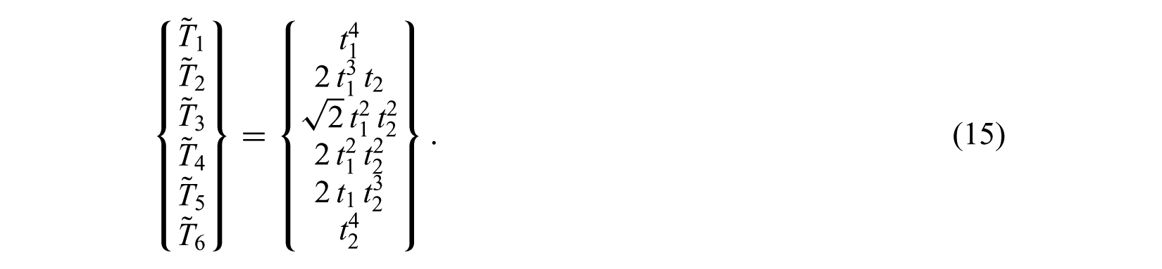
It is evident from this expression that one can construct a Euclidean-structure-preserving one-to-one mapping between the spaces $ℝ^{6}$ and $S_{4}^{2}$ by associating the vector $\tilde{C} = ({\tilde{C}}_{1}, {\tilde{C}}_{2}, {\tilde{C}}_{3}, {\tilde{C}}_{4}, {\tilde{C}}_{5}, {\tilde{C}}_{6}) \in ℝ^{6}$ to the ordered six-tuple

(C_{1111}, 2 C_{1112}, \sqrt{2} C_{1122}, 2 C_{1212}, 2 C_{1222}, C_{2222}) .

In particular, the vector $\tilde{T}$ in $ℝ^{6}$ associated with a unit tensor $t \otimes t \otimes t \otimes t$ is

{\begin{matrix} {\tilde{T}}_{1} \\ {\tilde{T}}_{2} \\ {\tilde{T}}_{3} \\ {\tilde{T}}_{4} \\ {\tilde{T}}_{5} \\ {\tilde{T}}_{6} \end{matrix}} = {\begin{matrix} t_{1}^{4} \\ 2 t_{1}^{3} t_{2} \\ \sqrt{2} t_{1}^{2} t_{2}^{2} \\ 2 t_{1}^{2} t_{2}^{2} \\ 2 t_{1} t_{2}^{3} \\ t_{2}^{4} \end{matrix}} .

(15)

We now check that

\tilde{T} \cdot \tilde{T} = {\tilde{T}}_{i} {\tilde{T}}_{i} = {(t_{1}^{2} + t_{2}^{2})}^{4} = 1,

(16)

thus confirming that our transformation of tensors into vectors indeed preserves the inner product.

3.3. Representation of uniaxial tensors

A uniaxial tensor $V \in S_{4}^{2}$ is a decomposable fourth-order tensor of the form

V = v \otimes v \otimes v \otimes v,

(17)

where $v \in ℝ^{2}$ . If $v \cdot v = 1$ , we say that $V$ is a unit uniaxial tensor. The collection $T$ of all unit uniaxial tensors is, clearly, generated by the radii of the unit circle in $ℝ^{2}$ . Thus, the representation of $T$ in $ℝ^{6}$ is a closed curve $Λ$ , which we call the hodographic guide.

According to equation (15), regardless of the vector $t$ of departure, we have

{\tilde{T}}_{4} = \sqrt{2} {\tilde{T}}_{3} .

(18)

By linearity, we conclude that all uniaxial tensors lie in a fixed (five-dimensional) hyperplane $ℋ$ containing the origin. We call $ℋ$ the fundamental hyperplane in $ℝ^{6}$ . In particular, the hodographic guide $Λ$ belongs to this hyperplane.

Moreover, for any unit uniaxial tensor $T$ , we have

{\tilde{T}}_{1} + {\tilde{T}}_{4} + {\tilde{T}}_{6} = t_{1}^{4} + 2 t_{1}^{2} t_{2}^{2} + t_{2}^{4} = {(t_{1}^{2} + t_{2}^{2})}^{2} = 1 .

(19)

In other words, the hodographic guide lies in the hyperplane $K$ with equation ${\tilde{T}}_{1} + {\tilde{T}}_{4} + {\tilde{T}}_{6} = 1$ . We may say, therefore, that the hodographic guide belongs to the four-dimensional plane $ℋ \cap K$ .

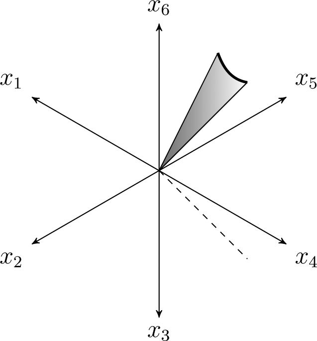
Consider now the collection $W$ of all non-zero uniaxial tensors. By linearity, since the only missing degree of freedom in $T$ is the multiplication by a positive scalar, we conclude that the collection $W$ is mapped onto the two-dimensional cone $C$ subtended by $Λ$ . (Recall that the cone subtended by a subset $S$ of a vector space is defined as the collection of all vectors of the form $α v$ , where $v \in S$ and $α \in ℝ^{+}$ .) We call $C$ the hodographic cone.

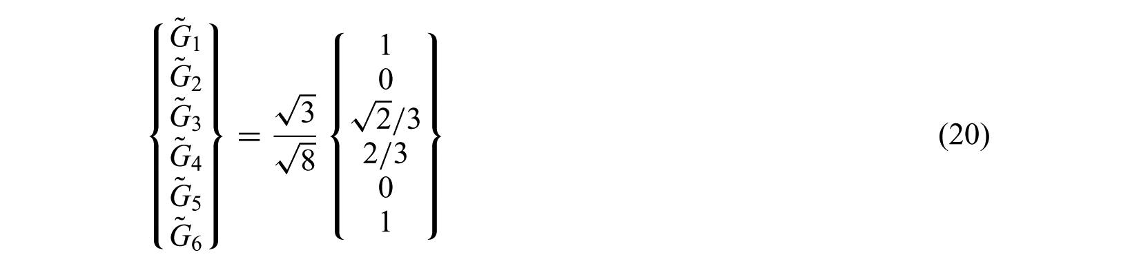
We note that the unit vector $\tilde{G}$ with components

{\begin{matrix} {\tilde{G}}_{1} \\ {\tilde{G}}_{2} \\ {\tilde{G}}_{3} \\ {\tilde{G}}_{4} \\ {\tilde{G}}_{5} \\ {\tilde{G}}_{6} \end{matrix}} = \frac{\sqrt{3}}{\sqrt{8}} {\begin{matrix} 1 \\ 0 \\ \sqrt{2} / 3 \\ 2 / 3 \\ 0 \\ 1 \end{matrix}}

(20)

belongs to $ℋ$ and forms a constant angle with all vectors $\tilde{V}$ arising from uniaxial tensors $V$ . Noting that a vector in the intersection $ℒ = K \cap ℋ$ must necessarily be of the form $〈 a, b, c, \sqrt{2} c, d, - (a + \sqrt{2} c) 〉$ , where $a, b, c, d$ are arbitrary real numbers, we conclude that $\tilde{G}$ is perpendicular to $ℒ$ . All the facts described above are summarized in the following lemma.

Lemma 3.2. The collection $W$ of all uniaxial fourth-order tensors in $ℝ^{2}$ is mapped onto a cone of revolution $C$ of dimension 2 in $ℋ$ whose axis is $\tilde{G}$ and whose normal cross section is $Λ$ .

3.4. Extension of the notion of hodograph to tensors

We will now extend the notion of hodograph to fourth-order tensor fields defined on plane curves. Let $Γ$ be a parametrized curve in $ℝ^{2}$ , as defined in equation (2). A tangential fourth-order tensor field $E (s)$ on $Γ$ , is a uniaxial tensor field of the form

E (s) = E (s) t (s) \otimes t (s) \otimes t (s) \otimes t (s),

(21)

where $E (s)$ is a sufficiently differentiable scalar field on $Γ$ . Note that $E (s) \in S_{4}^{2}$ and, from previous results, it uniquely corresponds to a curve $Λ_{E}$ with position vector

\tilde{E} = E (s) \tilde{T} (s),

(22)

where $\tilde{T} (s)$ has components of the form prescribed by equation (15). We call $Λ_{E}$ the hodograph of the tangential field $E (s)$ . We note that the hodograph may have cusps in correspondence with points of inflection of $Γ$ .

From the considerations of the previous section, we may state that all possible hodographs lie on the hodographic cone $C$ , as schematically represented in Figure 2.

Figure 2.

Schematic representation of the hodographic cone.

3.5. Projected fields

Consider a special type of tangential field $E (s)$ that arises from the Euclidean projection on $Γ$ of a constant field $ℂ \in S_{4}^{2}$ defined on a tubular neighbourhood of $Γ \subset ℝ^{2}$ , i.e.,

E (s) = ℂ \cdot (t (s) \otimes t (s) \otimes t (s) \otimes t (s)) = \tilde{C} \cdot \tilde{T},

(23)

where ${\tilde{C}}_{1} = C_{1111}$ , ${\tilde{C}}_{2} = 2 C_{1112}$ , ${\tilde{C}}_{3} = \sqrt{2} C_{1122}$ , ${\tilde{C}}_{4} = 2 C_{1212}$ , ${\tilde{C}}_{5} = 2 C_{1222}$ , and $C_{6} = C_{2222}$ .

By Lemmas 3.1 and 3.2, we obtain the following theorem.

Theorem 3.3. A tangential fourth-order tensor field $E (s)$ , defined on a curve $Γ$ in $ℝ^{2}$ , is the Euclidean projection of a constant $ℂ \in S_{4}^{2}$ if, and only if, its hodograph is in the intersection of the hodographic cone with a four-dimensional sphere passing through the origin and contained in the fundamental hyperplane.

Since a beam with axial elasticity $E (s)$ is homogeneously embeddable when the uniaxial tensor field $E (s)$ is the projection of a constant field, we have, by means of this theorem, characterized geometrically the homogeneity of embedding for linearly elastic beams. We seek now to further characterize this property and to define measures of inhomogeneity by means of differential geometric properties of curves in $ℝ^{n}$ .

3.6. Differential geometry of curves in $ℝ^{n}$

3.6.1. Generalized Serret–Frenet frames

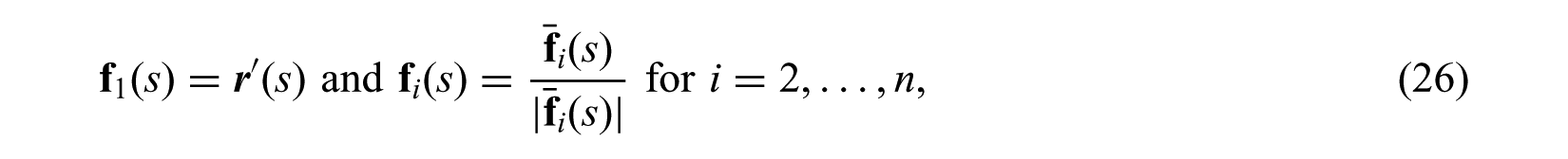
The Serret–Frenet formulation for curves in $ℝ^{3}$ has been generalized to curves in $ℝ^{n}$ by the French mathematician Camille Jordan in 1874 [6]. If $r (s) \in ℝ^{n}$ is an arc-length parametrized curve, with enough differentiability, then the set of $n$ vectors

{r' (s), r'' (s), \dots, r^{(n)} (s)},

(24)

if linearly independent, can be transformed into the orthonormal set of vectors

{f_{1} (s), f_{2} (s), \dots, f_{n} (s)},

(25)

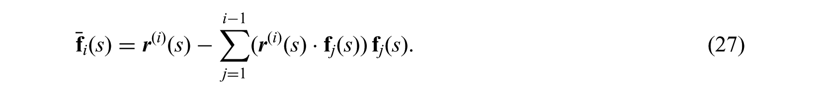
called the generalized Serret–Frenet frame, by the usual Gram–Schmidt process, where

f_{1} (s) = r' (s) and f_{i} (s) = \frac{{\bar{f}}_{i} (s)}{| {\bar{f}}_{i} (s) |} for i = 2, \dots, n,

(26)

and

{\bar{f}}_{i} (s) = r^{(i)} (s) - \sum_{j = 1}^{i - 1} (r^{(i)} (s) \cdot f_{j} (s)) f_{j} (s) .

(27)

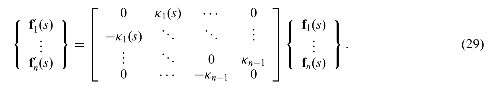
The generalized curvatures $κ_{i} (s)$ are defined as

κ_{i} (s) = f'_{i} (s) \cdot f_{i + 1} (s), i = 1, \dots, n - 1 .

(28)

Then the generalized Serret–Frenet formula, in matrix form, is

{\begin{matrix} f'_{1} (s) \\ ⋮ \\ f'_{n} (s) \end{matrix}} = [\begin{matrix} 0 & κ_{1} (s) & \dots & 0 \\ - κ_{1} (s) & ⋱ & ⋱ & ⋮ \\ ⋮ & ⋱ & 0 & κ_{n - 1} \\ 0 & \dots & - κ_{n - 1} & 0 \end{matrix}] {\begin{matrix} f_{1} (s) \\ ⋮ \\ f_{n} (s) \end{matrix}} .

(29)

The last generalized curvature $κ_{n - 1} (s)$ corresponds to the torsion of a space curve in $ℝ^{3}$ , because $κ_{n - 1} (s)$ being identically zero guarantees the curve to lie on a hyperplane and vice versa. If $f_{i} = 0$ , for some $i \leq n$ , we set $κ_{i - 1} = 0$ and the procedure comes to an end.

As an example, consider the hodographic guide $Λ$ . Using initially the slope-angle $θ$ of the unit vector $t$ as a parameter and differentiating equation (15), we find that the length parameter of $Λ$ (in $ℝ^{6}$ ) is $s = 2 θ$ . Carrying out the successive differentiations indicated in expression ((24)) and implementing the Gram–Schmidt procedure described thereafter, we observe that the process must be stopped at the fourth step, indicating that the original six vectors are not linearly independent. The curvatures are constant along the curve and have the values $κ_{1} = \sqrt{5 / 2}$ , $κ_{2} = (3 / 2) \sqrt{2 / 5}$ , $κ_{3} = 2 \sqrt{2 / 5}$ and $κ_{4} = 0$ . The fact that $f_{5} = 0$ (identically) implies that the curve lies in a four-dimensional plane (namely, $ℒ$ ), as we already knew. The fact that $κ_{3} \neq 0$ , however, constitutes additional information and implies that the hodographic guide $Λ$ does not lie in a lower dimensional plane.

Curves of constant curvatures in $ℝ^{4}$ have been studied in detail by [7, 8]. It can be shown that these curves lie on a four-sphere of radius

R = \frac{\sqrt{κ_{2}^{2} + κ_{3}^{2}}}{| κ_{1} κ_{3} |} .

(30)

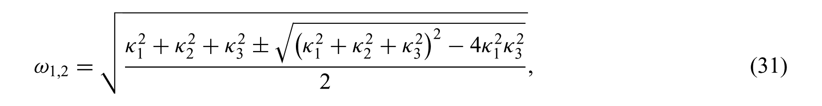
For the particular values of our curvatures, we obtain that $R = 1 / κ_{3}$ . Moreover, general curves of constant curvature can be regarded as the superposition of two harmonic functions with different frequencies, $ω_{1}$ and $ω_{2}$ . Much in the same way as for Lissajous figures, these curves are closed if, and only if, the ratio between the two characteristic frequencies is rational. The frequencies are given by the formula

ω_{1, 2} = \sqrt{\frac{κ_{1}^{2} + κ_{2}^{2} + κ_{3}^{2} \pm \sqrt{{(κ_{1}^{2} + κ_{2}^{2} + κ_{3}^{2})}^{2} - 4 κ_{1}^{2} κ_{3}^{2}}}{2}},

(31)

which, for the particular case of our $Λ$ , yields

ω_{1} = 2 ω_{2} = 1,

(32)

thus confirming the obvious fact that, as defined by equation (15), the hodographic guide is indeed a closed curve (rather than a curve winding itself densely around a spherical zone).

3.6.2. Order of contact and osculating sphere

Let $F : ℝ^{n} \to ℝ$ be a sufficiently smooth function which has a regular value zero. Then, it is known that $F^{- 1} (0)$ is a hyper-surface, i.e. a submanifold of dimension ( $n - 1$ ), of $ℝ^{n}$ . The curve $r (s)$ is said to have order $k$ contact at $r (s_{0})$ with a hyper-surface $F^{- 1} (0)$ if

(F \circ r) (s_{0}) = (F \circ r)' (s_{0}) = \dots = {(F \circ r)}^{(k)} (s_{0}) = 0,

but ${(F \circ r)}^{(k + 1)} (s_{0}) \neq 0$ . This definition is independent of parametrization. The osculating sphere at $r (s_{0})$ is the unique hyper-sphere with which the curve has order $(n + 1)$ contact at $r (s_{0})$ . It has been shown [9] that, provided all $κ_{i} (s_{0})$ are non-zero, the center of the osculating sphere at $r (s_{0})$ lies at

a (s_{0}) = r (s_{0}) + m (s_{0}),

(33)

where $m (s_{0}) = m_{i} (s) f_{i} (s_{0})$ , with, $m_{i} (s), i = 1, \dots, n$ , being the curvature functions of $r (s)$ , defined as

m_{i} (s) = {\begin{matrix} 0, & i = 1 \\ \frac{1}{κ_{1} (s)}, & i = 2 \\ \frac{{m^{'}}_{i - 1} (s) + m_{i - 2} (s) κ_{i - 2} (s)}{κ_{i - 1} (s)}, & i = 3, \dots, n, \end{matrix}}

and, its radius is $| m (s_{0}) |$ . Further, the osculating sphere at $r (s_{0})$ passes through the origin if $a (s_{0}) \cdot a (s_{0}) - {| m (s_{0}) |}^{2} = 0$ , or

{| r (s_{0}) |}^{2} + 2 r (s_{0}) \cdot m (s_{0}) = 0 .

(34)

3.6.3. Sphericity of curves

The curve $r (s)$ is spherical, i.e. lies on a hyper-sphere, if the locus of the centres of the osculating spheres along the curve is a point. The necessary and sufficient condition [9] for this to happen, assuming sufficient smoothness of $r (s)$ and no $κ_{i} (s)$ zero for any $s$ , is that

m'_{n} + m_{n - 1} κ_{n - 1} = 0

(35)

identically. Note that this condition guarantees contacts of at least order $(n + 2)$ with the hyper-sphere at all points on the curve. We say that the curve is locally spherical at a point $r (s_{0})$ if (35) is satisfied at $s_{0}$ .

Note 2. If the curve $r (s)$ is hyper-planar, i.e. if $κ_{n - 1} = 0$ identically, then $κ_{n - 1}$ and $m_{n}$ do not appear in the above conditions. Also, the definition of the osculating sphere only demands contact of order $n$ and sphericity of a curve demands contacts of order at least $(n + 1)$ at all points.

If $r (s_{0})$ is the hyper-planar hodograph $ℰ$ in $ℝ^{6}$ of an everywhere non-vanishing tangential field $E (s) \in S_{4}^{2}$ , then the condition (34) reduces to

E (s_{0}) + 2 \tilde{T} (s_{0}) \cdot m (s_{0}) = 0 .

(36)

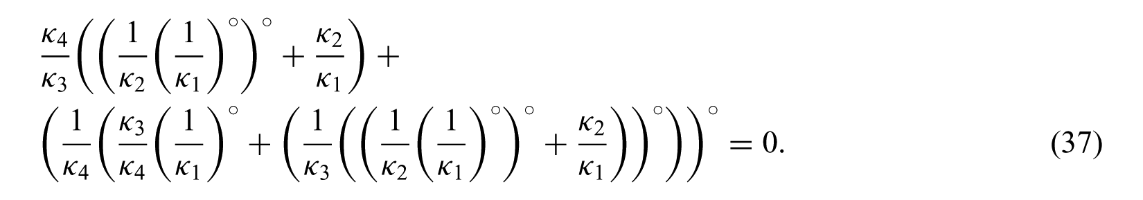
The condition of local sphericity of the hodograph at some $s_{0}$ explicitly reads

\begin{matrix} \frac{κ_{4}}{κ_{3}} ({(\frac{1}{κ_{2}} {(\frac{1}{κ_{1}})}^{\circ})}^{\circ} + \frac{κ_{2}}{κ_{1}}) + \\ {(\frac{1}{κ_{4}} (\frac{κ_{3}}{κ_{4}} {(\frac{1}{κ_{1}})}^{\circ} + {(\frac{1}{κ_{3}} ({(\frac{1}{κ_{2}} {(\frac{1}{κ_{1}})}^{\circ})}^{\circ} + \frac{κ_{2}}{κ_{1}}))}^{\circ}))}^{\circ} = 0 . \end{matrix}

(37)

In this equation, we have used the superscript $\circ$ to indicate differentiation with respect to the arc-length parameter measured along the hodograph, which is in general different from the length parameter along the original curve $Γ$ .

Note 3. Measure of embedded inhomogeneity: Let the axis of a planar elastic beam be given by the arc-length parametrized curve $r = r (s)$ , and let $E (s)$ be the elastic modulus satisfying equations (3) and (4). Assuming sufficient smoothness of $r (s)$ and $E (s)$ so that all the generalized curvatures $κ_{i} (s)$ of the hodograph $ℰ$ , except $κ_{5} (s)$ , are non-zero and sufficiently smooth, a non-zero value of the left-hand side of (36) at $s_{0}$ provides a measure of local embedded inhomogeneity of the beam at $s_{0}$ , provided (37) is satisfied thereat.

4. Final thoughts on embedded homogeneity

A planar beam is a slender solid body in which one dimension (the beam axis) predominates over the other two (the cross section). If the beam is linearly elastic, its constitutive response is expressed in terms of linear relations between stresses and strains. The question we ask is whether a given stress-free configuration of the rod is homogeneous or not. Given a small sample of the beam, a material scientist would not take into consideration any theorized one-dimensional model of the original three-dimensional beam, but rather look for any detectable presence, under the microscope, of micro-structural defects in the solid rod.

But in classical structural theories, a linearly elastic beam is understood as a pair of objects, namely, a curve $Γ$ and an elasticity modulus field $E (s)$ to be entered in equations such as ((3)) and ((4)). To give a mathematical representation of the physical idea of homogeneity, rather than that of the mathematical construct arising from the structural one-dimensional model, we proposed the notion of embedded homogeneity. In simple terms, we state that a planar beam is physically homogeneous if the plane curve $Γ$ can be embedded into a homogeneous planar elastic domain in such a way that, after performing the standard thickness-wise integration of the stresses, we recover the given structural model. The conditions for this kind of homogeneity, namely the physically observable one, consist of a subtle interplay between the geometry of the curve, on the one hand, and the elastic modulus field, on the other. When expressed analytically, these conditions can be encompassed in the vanishing of a sixth-order Wronskian determinant involving the function $E (s)$ and five fixed basis functions arising from the shape of the beam axis.

As expected in a theory of continuous distributions of defects, the homogeneity conditions bear also a differential-geometric interpretation. A surprising feature of this interpretation is the appearance of the hodograph curve in $ℝ^{6}$ associated with an isometric vectorial representation of the inner-product space of symmetric fourth-order tensors in $ℝ^{2}$ . It turns out that a curve in $ℝ^{2}$ gives rise to a two-dimensional cone in $ℝ^{6}$ which is the carrier of the hodographs associated with all possible uniaxial fourth-order tangent tensor fields defined on that curve. A no less surprising feature of the geometric interpretation is that the beam is physically homogeneous if, and only if, its hodograph belongs to a four-dimensional sphere containing the origin of $ℝ^{6}$ . On the basis of this result, it is possible to construct local measures of inhomogeneity by measuring both the degree of contact of the curve with its osculating sphere and the distance of this sphere from the origin. The generalization of these ideas to spatial beams and to shells, while fraught with difficulties, will follow similar lines and open new perspectives in the field of dislocation theory.

Footnotes

Funding

The authors gratefully acknowledge the support of the Natural Sciences and Engineering Research Council of Canada and the Shastri Indo-Canadian Institute.

References

Wang

C-C

. Material uniformity and homogeneity in shells. Arch Ration Mech Anal 1972; 47: 343–368.

Epstein

De León

. On uniformity of shells. Int J Sol Struct 1998: 35(17): 2173–2182.

Steigmann

. Fluid films with curvature elasticity. Arch Ration Mech Anal 1999: 150(2): 127–152.

Eremeyev

Pietraszkiewicz

. Local symmetry group in the general theory of elastic shells, J Elasticity 2006; 85(2): 125–152.

Šilhavý

. The Mechanics and Thermodynamics of Continuous Media. New York: Springer-Verlag, 1997.

Jordan

. Sur la théorie des courbes dans l’espace àn dimensions, C R Acad Sci Paris 1874; 79: 795–797.

Yew

. Curves in four-dimensional space, www.sms.math.nus.edu.sg.

Nalty

. Curves of constant curvatures in four dimensional spacetime, www.kurtnalty.com/ThreeCurvatures.pdf, pp.1–31, 2011.

Ozdamar

Hacisalihoglu

. Characterization of spherical curves in Euclidean n-space, Comm Fac Sci Univ Ankara 1974; 23A: 122–124.