Weak solvability via Lagrange multipliers for contact problems involving multi-contact zones

Abstract

We investigate the behaviour of an elastic body which is in frictional contact with a foundation on a part of the boundary, and which can come into contact with a rigid obstacle on another part of the boundary. We associate this physical setting with two mechanical models. Every model is mathematically described by a boundary value problem which consists of a system of partial differential equations associated with a displacement condition, a traction condition, a frictional contact condition and a frictionless unilateral contact condition. In both models the unilateral contact is described by Signorini’s condition with non-zero gap. The difference between the models is given by the frictional condition we use. In the first model we use a condition with prescribed normal stress. In the second one, we use a frictional bilateral contact condition. The weak solvability of the boundary value problems we propose herein relies on an abstract generalized saddle point problem. Abstract existence, uniqueness and boundedness results as well as abstract convergence results of a regularization are established. Then, we discuss the existence, the uniqueness, the boundedness and the approximation of the weak solutions based on the abstract results.

Keywords

Contact models friction laws prescribed normal stress bilateral contact unilateral contact Lagrange multipliers mixed variational formulation weak solution existence regularized problem approximation

1. Introduction

Contact between bodies is a customary phenomenon. However, the mathematical handling of the contact models requires complex knowledge about mathematical modelling in contact mechanics, starting with elements of mechanics of continua, using techniques in nonlinear analysis, variational calculus, numerical analysis, and going on to computation. Let us indicate a few useful references. For mathematical modelling in contact mechanics we refer the reader to, for example, [1 –9]; herein the reader can find various contact models as well as their analysis. The reader interested in computational contact mechanics can go for instance to [10, 11]. For some useful mathematical tools we send the reader to, for example, [12 –15]. Due to the complexity of contact models, their solvability relies on variational calculus. Thus, along the years the weak solvability in contact mechanics was related to various kinds of variational inequalities. In the last years several papers were devoted to the weak solvability via dual Lagrange multipliers of contact models; see for example [16 –22] for qualitative analysis and [23 –30] for modern numerical approaches.

The present paper focuses on the weak solvability via Lagrange multipliers for contact problems involving two contact zones. Precisely, we investigate the behaviour of an elastic body which, on a part of the boundary is in frictional contact with a foundation and at the same time on another part of the boundary it can come in contact with a rigid obstacle. We analyse two models. Every model is mathematically described by a boundary value problem which consists of a system of partial differential equations associated with a displacement condition, a traction condition, a frictional contact condition and a frictionless unilateral contact condition. Two types of frictional contact conditions are involved in the present work: the first one is a frictional contact condition with prescribed normal stress and the second one is a frictional bilateral contact condition. In order to model the unilateral contact we shall use the Signorini condition with non-zero gap.

The models we investigate in the present paper are not multi-body contact problems because they involve only one deformable body; commonly, the contact models involving more than one deformable body are called ‘multi-body contact problems’ in the literature. However, the models we treat involve more than one contact zone. Moreover, the technique used in this work allows us to generalize the present study to the case of more than two contact zones; this motivates the title of the paper.

The solvability of the boundary value problems we propose herein relies on abstract generalized saddle point problems. A first step in the study of such an abstract problem was made in [31]. In the present work we improve and extend the results in [31] focusing on applications of the abstract results to the weak solvability for contact problems involving multi-contact zones.

In Section 2 we deliver abstract existence, uniqueness, boundedness and approximation results. In Section 3 we state the models and hypotheses. In Section 4 we discuss the existence, the uniqueness, the boundedness and the approximation of the weak solutions based on Section 2.

We end this introductory section by recalling some elements of convex analysis in Hilbert spaces.

A functional $ϕ : X \to ℝ$ is Gâteaux differentiable at u if there exists ∇ϕ(u) ∈ X so that

\lim_{t \to 0} \frac{ϕ (u + t v) - ϕ (u)}{t} = {(\nabla ϕ (u), v)}_{X} for all v \in X .

The element ∇ϕ(u) is called the gradient of ϕ at u. The functional ϕ is Gâteaux differentiable if it is Gâteaux differentiable at every point u ∈ X. Also, recall that $ϕ : X \to ℝ$ is convex if

ϕ ((1 - λ) x + λ y) \leq (1 - λ) ϕ (x) + λ ϕ (y),

for all x,y ∈ X and λ ∈ (0, 1).

Proposition 1. Let $ϕ : X \to ℝ$ be a Gâteaux differentiable functional. Then, ϕ is a convex functional if and only if

ϕ (v) - ϕ (u) \geq {(\nabla ϕ (u), v - u)}_{X} f o r a l l v \in X .

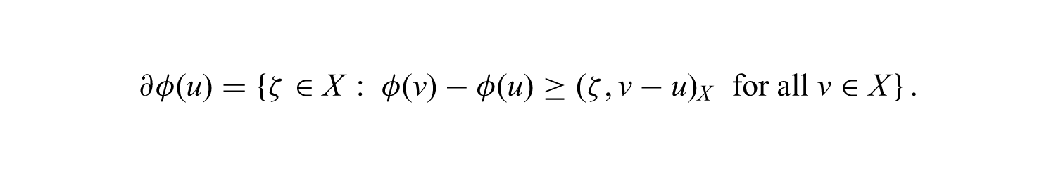
The subdifferential of a functional ϕ: X → (−∞, +∞] at a point u ∈{v ∈ X:ϕ(v) < ∞} is the (possibly empty) set

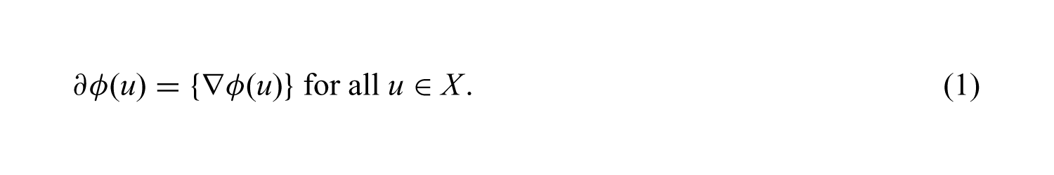
\partial ϕ (u) = {ζ \in X : ϕ (v) - ϕ (u) \geq {(ζ, v - u)}_{X} for all v \in X} .

It is worth recalling that, if $ϕ : X \to ℝ$ is convex and Gâteaux differentiable, then

\partial ϕ (u) = {\nabla ϕ (u)} for all u \in X .

(1)

Further details can be found for instance in [32, 33].

We now recall some elements of saddle point theory. Since the saddle point of a functional is the key of the variational approaches via Lagrange multipliers, we start by recalling its definition.

Definition 1. Let A and B be two non-empty sets. A pair (u, λ) ∈ A × B is said to be a saddle point of a functional $ℒ : A \times B \to ℝ$ if and only if

ℒ (u, μ) \leq ℒ (u, λ) \leq ℒ (v, λ), f o r a l l v \in A, μ \in B .

The following existence result is also a basic tool of the variational approaches via Lagrange multipliers; see [32].

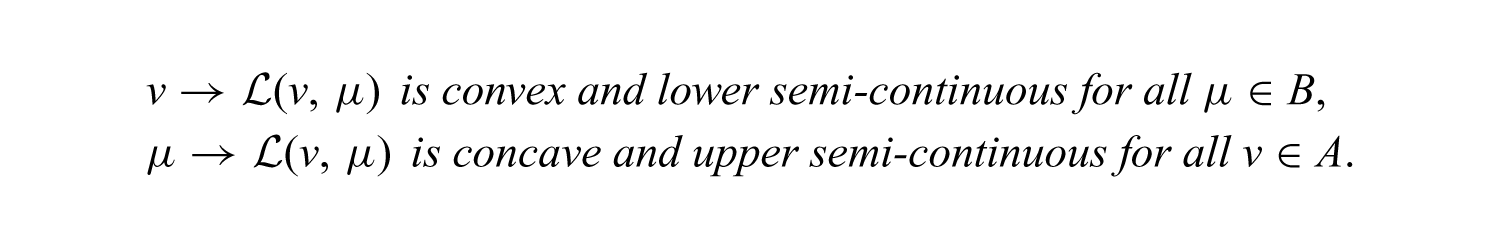
Theorem 1. Let (X,(·,·)_X,∥·∥_X), (Y,(·,·)_Y,∥·∥_Y) be two Hilbert spaces and let A ⊆ X, B ⊆ Y be non-empty, closed, convex subsets. Assume that a real functional $ℒ : A \times B \to ℝ$ satisfies the following conditions:

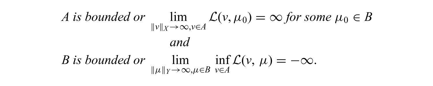
\begin{array}{l} v \to ℒ (v, μ) i s c o n v e x a n d l o w e r s e m i - c o n t i n u o u s f o r a l l μ \in B, \\ μ \to ℒ (v, μ) i s c o n c a v e a n d u p p e r s e m i - c o n t i n u o u s f o r a l l v \in A . \end{array}

Moreover, assume that

\begin{array}{l} A i s b o u n d e d o r & \lim_{‖ v ‖_{X} \to \infty, v \in A} ℒ (v, μ_{0}) = \infty f o r s o m e μ_{0} \in B \\ a n d \\ B i s b o u n d e d o r & \lim_{‖ μ ‖_{Y} \to \infty, μ \in B} \inf_{v \in A} ℒ (v, μ) = - \infty . \end{array}

Then, the functional $ℒ$ has at least one saddle point (u, λ) ∈ A × B. If $ℒ$ is strictly convex in the first argument, then the saddle point is unique in the first argument; if $ℒ$ is strictly concave in the second argument then the saddle point is unique in the second argument.

For a more complex view on the saddle point theory, we refer the reader to [32, 34 –37] and to the related references therein. Also, we would like to refer to [3, 38] for existence and uniqueness results in contact mechanics based on saddle point formulations.

Some arguments we use are standard or have been used in other works related to the topic being discussed; we present them in order to have a self-contained paper, easy to read.

2. Abstract auxiliary results

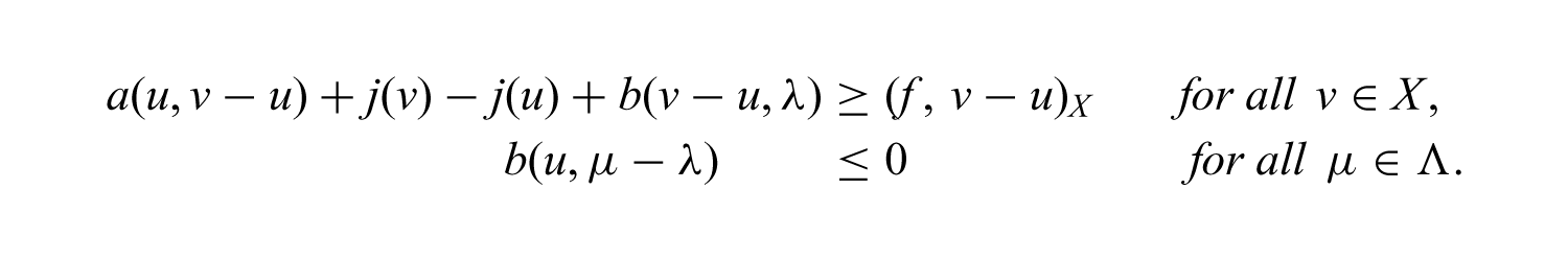
Let (X, (·,·)_X, ∥·∥_X) and (Y, (·,·)_Y, ∥·∥_Y) be two real Hilbert spaces and Λ ⊂ Y. We focus on the following problem.

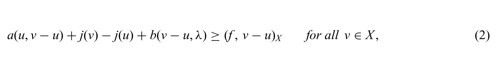
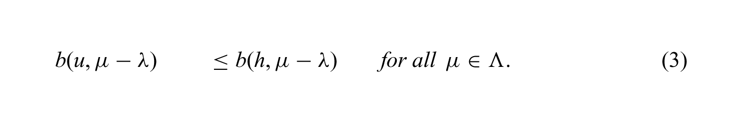
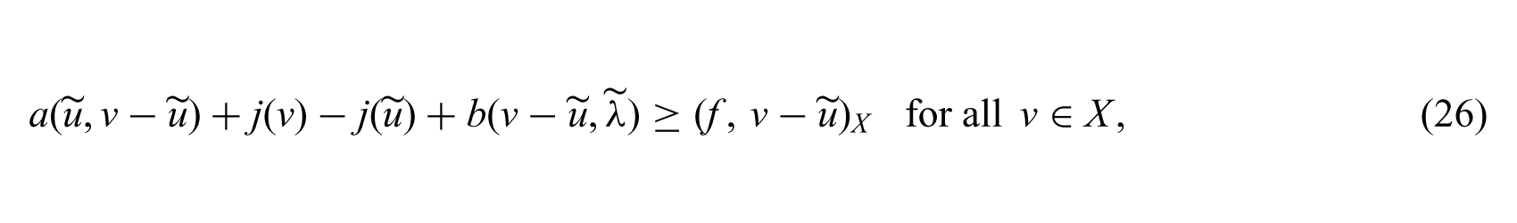
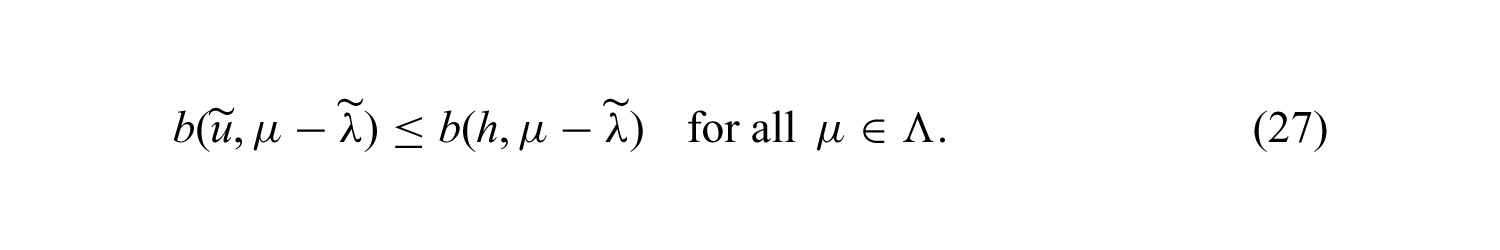
Problem 1. Given f, h ∈ X, find (u, λ) ∈ X × Y such that λ ∈ Λ and

a (u, v - u) + j (v) - j (u) + b (v - u, λ) \geq {(f, v - u)}_{X} f o r a l l v \in X,

(2)

b (u, μ - λ) \leq b (h, μ - λ) f o r a l l μ \in Λ .

(3)

A first step in the study of Problem 1 was made in [31]; there the well-posedness of Problem 1 for the case j(0_X) = 0 was investigated. In this paper we do not impose this restriction. We study the existence, uniqueness and boundedness of the solutions focusing on the uniqueness of the solution on the first argument. Also, we consider a regularized problem for which we get existence, uniqueness and boundedness results. Besides, we prove convergence results which help us to arrive at a solution to Problem 1 starting from a sequence of solutions of a sequence of regularized problems.

2.1. Existence, uniqueness and boundedness results

Let us make the following assumptions.

Assumption 1. $a (\cdot, \cdot) : X \times X \to ℝ$ is a symmetric bilinear form such that:

(i₁) There exists M_a > 0: |a(u, v)| ≤ M_a∥u∥_X∥v∥_X for all u,v ∈ X;

$(i_{2}) T h e r e e x i s t s m_{a} > 0 : a (v, v) \geq m_{a} ‖ v ‖_{X}^{2} f o r a l l v \in X .$

Assumption 2. The functional $j : X \to ℝ$ is convex. In addition, there exists L_j > 0 such that

| j (v) - j (u) | \leq L_{j} ‖ v - u ‖_{X} f o r a l l u, v \in X .

Assumption 3. $b (\cdot, \cdot) : X \times Y \to ℝ$ is a bilinear form such that:

(j₁) There exists M_b > 0: |b(v, μ)|≤M_b∥v∥_X∥μ∥_Y for all v ∈ X, μ ∈ Y;

(j₂) There exists

α > 0 : \inf_{μ \in Y, μ \neq 0_{Y}} \sup_{v \in X, v \neq 0_{X}} \frac{b (v, μ)}{‖ v ‖_{X} ‖ μ ‖_{Y}} \geq α .

Assumption 4. Λ is a closed convex subset of Y such that 0_Y ∈Λ.

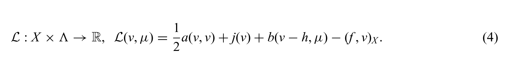
Let us define a functional $ℒ$ as follows:

ℒ : X \times Λ \to ℝ, ℒ (v, μ) = \frac{1}{2} a (v, v) + j (v) + b (v - h, μ) - {(f, v)}_{X} .

(4)

Lemma 1. The functional $ℒ$ admits at least one saddle point (u, λ) ∈ X ×Λ.

Proof. The map $v \to ℒ (v, μ)$ is convex and lower semi-continuous for every μ ∈ Λ. In addition, for every v ∈ X, the map $μ \to ℒ (v, μ)$ is concave and upper semi-continuous. On the other hand,

\lim_{‖ v ‖_{X} \to \infty, v \in X} ℒ (v, 0_{Y}) = \infty .

If Λ is a bounded set we shall apply Theorem 1.

Else, it is necessary to verify that

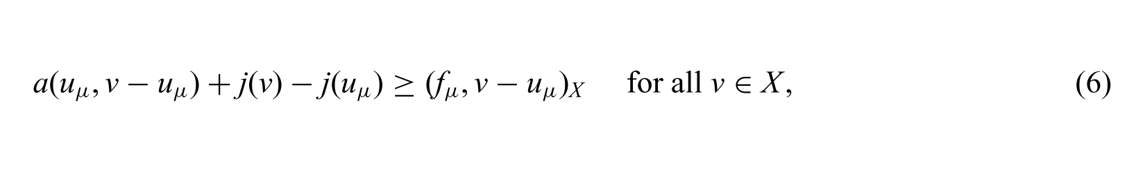
\lim_{‖ μ ‖_{Y} \to \infty, μ \in Λ} \inf_{v \in X} ℒ (v, μ) = - \infty .

(5)

To this end, let μ be an arbitrary element in Λ and let u_μ ∈ X be the unique solution of the variational inequality of the second kind

a (u_{μ}, v - u_{μ}) + j (v) - j (u_{μ}) \geq {(f_{μ}, v - u_{μ})}_{X} for all v \in X,

(6)

where f_μ ∈ X is defined using Riesz’s representation theorem as follows:

{(f_{μ}, v)}_{X} = {(f, v)}_{X} - b (v, μ) for all v \in X .

Obviously,

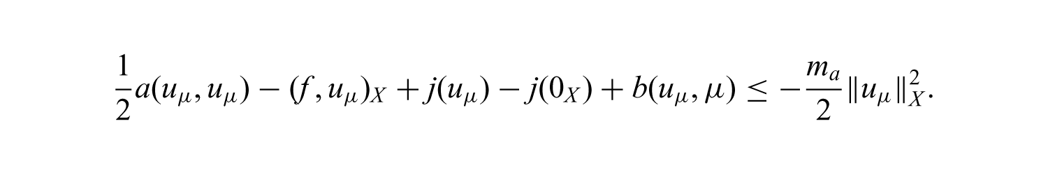
\inf_{v \in X} ℒ (v, μ) = \frac{1}{2} a (u_{μ}, u_{μ}) + j (u_{μ}) - {(f, u_{μ})}_{X} + b (u_{μ}, μ) - b (h, μ) .

Let us put v = 0_X in (6). Then, after summing with $\frac{1}{2} a (u_{μ}, u_{μ}),$ we deduce

\frac{1}{2} a (u_{μ}, u_{μ}) - {(f, u_{μ})}_{X} + j (u_{μ}) - j (0_{X}) + b (u_{μ}, μ) \leq - \frac{m_{a}}{2} ‖ u_{μ} ‖_{X}^{2} .

Therefore,

\inf_{v \in X} ℒ (v, μ) \leq - \frac{m_{a}}{2} ‖ u_{μ} ‖_{X}^{2} - b (h, μ) + j (0_{X}) .

Setting v = u_μ−w in (6) with w ∈ X, it follows that

b (w, μ) \leq {(f, w)}_{X} - a (u_{μ}, w) + j (u_{μ} - w) - j (u_{μ}) .

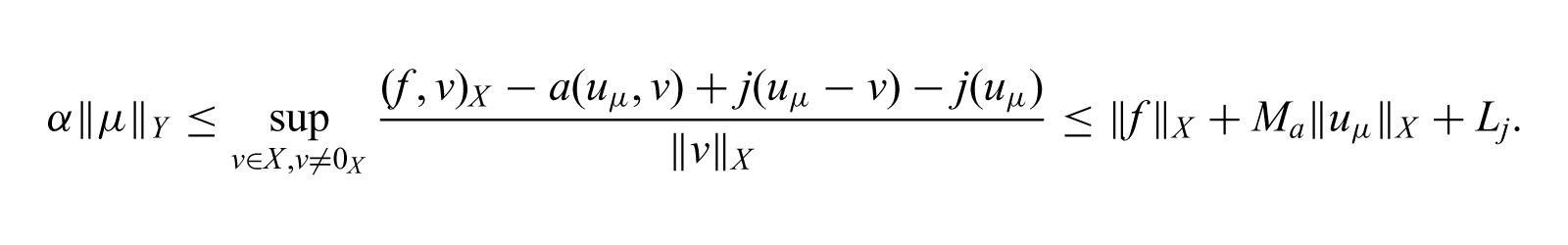
Due to the inf–sup property of the form b, we deduce that there exists α > 0 such that

α ‖ μ ‖_{Y} \leq \sup_{v \in X, v \neq 0_{X}} \frac{b (v, μ)}{‖ v ‖_{X}} .

Hence,

α ‖ μ ‖_{Y} \leq \sup_{v \in X, v \neq 0_{X}} \frac{{(f, v)}_{X} - a (u_{μ}, v) + j (u_{μ} - v) - j (u_{μ})}{‖ v ‖_{X}} \leq ‖ f ‖_{X} + M_{a} ‖ u_{μ} ‖_{X} + L_{j} .

Therefore, there exists c > 0 such that

‖ μ ‖_{Y}^{2} \leq c (‖ f ‖_{X}^{2} + ‖ u_{μ} ‖_{X}^{2} + L_{j}^{2}) .

Furthermore, there exists $\tilde{c} > 0$ such that

\inf_{v \in X} ℒ (v, μ) \leq - \tilde{c} (‖ μ ‖_{Y}^{2} - ‖ f ‖_{X}^{2} - L_{j}^{2}) + M_{b} ‖ h ‖_{X} ‖ μ ‖_{Y} + | j (0_{X}) | .

Since μ was arbitrarily fixed in Λ, by passing to the limit as ∥μ∥_Y → ∞, we obtain (5).

Consequently, based on Theorem 1, we deduce that the functional $ℒ$ has at least one saddle point. As $ℒ$ is strictly convex in the first argument we deduce that this functional has a saddle point which is unique in the first argument.

Theorem 2. (An existence and uniqueness result). If Assumptions 1 to 4 hold, then Problem 1 has at least one solution, unique in the first argument.

Proof. By standard arguments it can be proved that a pair (u, λ) ∈ X × Λ verifies (2)–(3) only if it is a saddle point of the functional $ℒ$ ; see for instance the proof of Lemma 3.1 in [31].

Taking into consideration Lemma 1 we conclude that Problem 1 has a solution which is unique in the first argument.

Proposition 2. (A boundedness result). Assumptions 1 to 4 hold. If (u, λ) ∈ X × Λ is a solution of Problem 1, then there exist K₁, K₂ > 0 such that

‖ u ‖_{X} \leq K_{1}; ‖ λ ‖_{Y} \leq K_{2} .

(7)

Proof. Let (u, λ) ∈ X × Λ be a solution of Problem 1. Setting v = 0_X in (2) we obtain

a (u, u) \leq {(f, u)}_{X} - j (u) + j (0_{X}) - b (u, λ) .

Now setting μ = 0_Y in (3), we get

- b (u, λ) \leq - b (h, λ) .

Hence,

m_{a} ‖ u ‖_{X}^{2} \leq a (u, u) \leq ‖ f ‖_{X} ‖ u ‖_{X} + L_{j} ‖ u ‖_{X} + M_{b} ‖ h ‖_{X} ‖ λ ‖_{Y} .

(8)

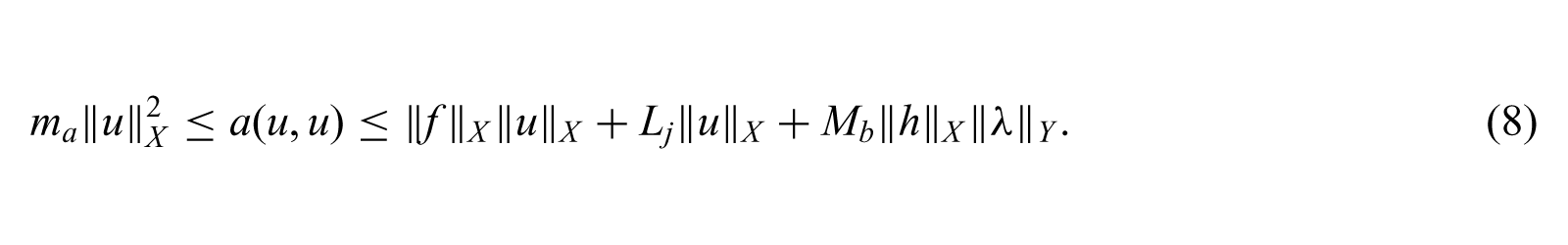
On the other hand, setting in (2) v = u−w with w an arbitrary element of X, we obtain

b (w, λ) \leq | {(f, w)}_{X} | + | j (u - w) - j (u) | + | a (u, w) | .

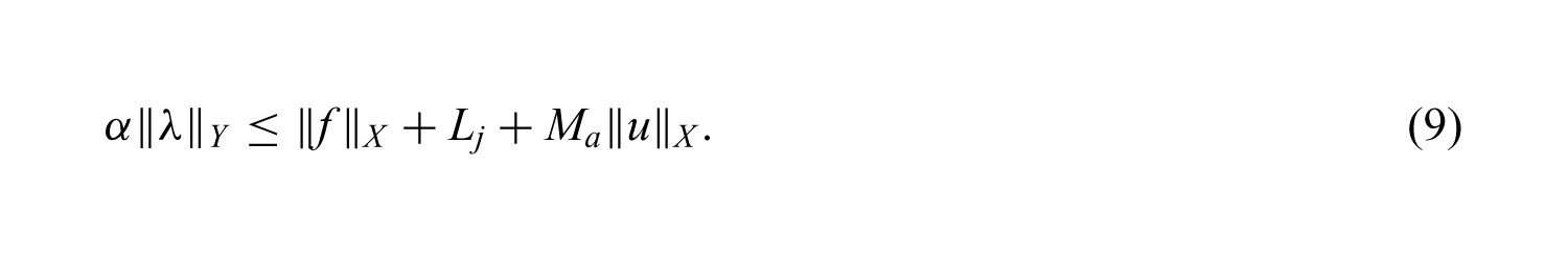
Using the inf–sup property of the form b and taking into account the Lipschitz property of the functional j as well as the continuity of the bilinear form a it follows that

α ‖ λ ‖_{Y} \leq ‖ f ‖_{X} + L_{j} + M_{a} ‖ u ‖_{X} .

(9)

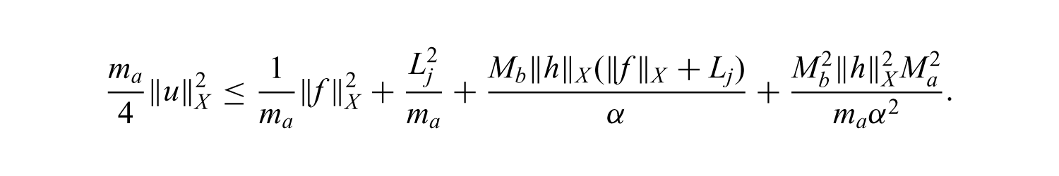
By (8) and (9) we obtain

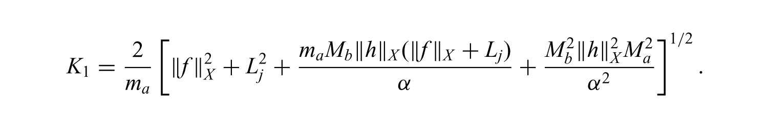
\begin{array}{l} m_{a} ‖ u ‖_{X}^{2} \leq \frac{1}{m_{a}} ‖ f ‖_{X}^{2} + \frac{m_{a}}{4} ‖ u ‖_{X}^{2} + \frac{L_{j}^{2}}{m_{a}} + \frac{m_{a}}{4} ‖ u ‖_{X}^{2} \\ + \frac{M_{b} ‖ h ‖_{X} (‖ f ‖_{X} + L_{j})}{α} + \frac{M_{b}^{2} ‖ h ‖_{X}^{2} M_{a}^{2}}{m_{a} α^{2}} + \frac{m_{a}}{4} ‖ u ‖_{X}^{2} . \end{array}

Furthermore,

\frac{m_{a}}{4} ‖ u ‖_{X}^{2} \leq \frac{1}{m_{a}} ‖ f ‖_{X}^{2} + \frac{L_{j}^{2}}{m_{a}} + \frac{M_{b} ‖ h ‖_{X} (‖ f ‖_{X} + L_{j})}{α} + \frac{M_{b}^{2} ‖ h ‖_{X}^{2} M_{a}^{2}}{m_{a} α^{2}} .

Let us take

K_{1} = \frac{2}{m_{a}} {[‖ f ‖_{X}^{2} + L_{j}^{2} + \frac{m_{a} M_{b} ‖ h ‖_{X} (‖ f ‖_{X} + L_{j})}{α} + \frac{M_{b}^{2} ‖ h ‖_{X}^{2} M_{a}^{2}}{α^{2}}]}^{1 / 2} .

By (9) we now get

‖ λ ‖_{Y} \leq \frac{1}{α} (‖ f ‖_{X} + L_{j} + M_{a} K_{1}) .

Hence, we can take

K_{2} = \frac{1}{α} (‖ f ‖_{X} + L_{j} + M_{a} K_{1}) .

Notice that, setting h = 0_X, Problem 1 leads us to the following semi-homogeneous problem.

Problem 2. Given f ∈ X, find (u, λ) ∈ X × Y such that λ ∈ Λ and

\begin{matrix} a (u, v - u) + j (v) - j (u) + b (v - u, λ) & \geq & {(f, v - u)}_{X} f o r a l l v \in X, \\ b (u, μ - λ) & \leq & 0 f o r a l l μ \in Λ . \end{matrix}

Using arguments similar to those used to prove Theorem 2 and Proposition 2, but with more simple writing, we get the following result.

Corollary 1. If Assumptions 1 to 4 hold, then Problem 2 has at least one solution, unique in the first argument. In addition,

\begin{matrix} ‖ u ‖_{X} & \leq & \frac{1}{m_{a}} (‖ f ‖_{X} + L_{j}); \\ ‖ λ ‖_{Y} & \leq & \frac{1}{α} (1 + \frac{M_{a}}{m_{a}}) (‖ f ‖_{X} + L_{j}) . \end{matrix}

2.2. A convergence result

Let ρ be a real positive number and $j_{ρ} : X \to ℝ$ be a functional which fulfills the following assumption.

Assumption 5. The functional $j_{ρ} : X \to ℝ$ is convex. In addition:

There exists a positive real number L, which is independent of ρ, such that

| j_{ρ} (v) - j_{ρ} (u) | \leq L ‖ v - u ‖_{X} f o r a l l u, v \in X .

j_ρ is a Gâteaux differentiable functional.

Let us denote by ∇j_ρ the Gâteaux differential of j_ρ.

Assumption 6.

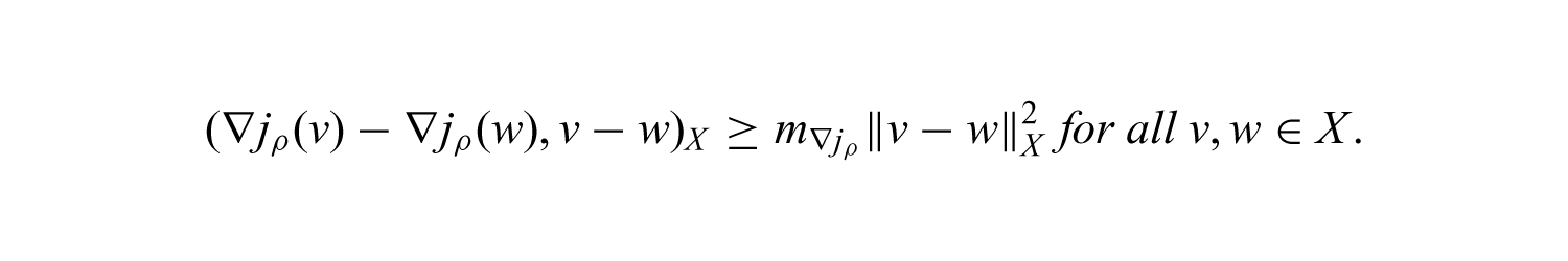
There exists L_∇jρ > 0 such that

‖ \nabla j_{ρ} (v) - \nabla j_{ρ} (w) ‖_{X} \leq L_{\nabla j_{ρ}} ‖ v - w ‖_{X} f o r a l l v, w \in X .

There exists m_∇jρ > 0 such that

{(\nabla j_{ρ} (v) - \nabla j_{ρ} (w), v - w)}_{X} \geq m_{\nabla j_{ρ}} ‖ v - w ‖_{X}^{2} f o r a l l v, w \in X .

Let us state the following regularized problem.

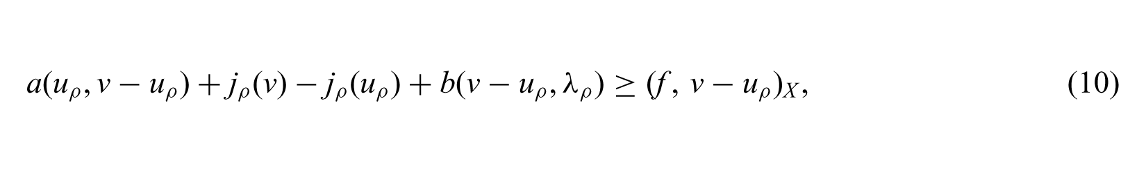
Problem 3. Given ρ > 0 and f, h ∈ X, find (u_ρ, λ_ρ) ∈ X × Y such that λ_ρ ∈ Λ ⊂ Y and, for all v ∈ X, μ ∈Λ,

a (u_{ρ}, v - u_{ρ}) + j_{ρ} (v) - j_{ρ} (u_{ρ}) + b (v - u_{ρ}, λ_{ρ}) \geq {(f, v - u_{ρ})}_{X},

(10)

b (u_{ρ}, μ - λ_{ρ}) \leq b (h, μ - λ_{ρ}) .

(11)

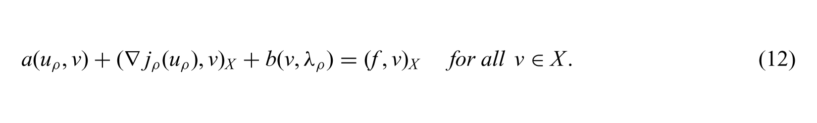
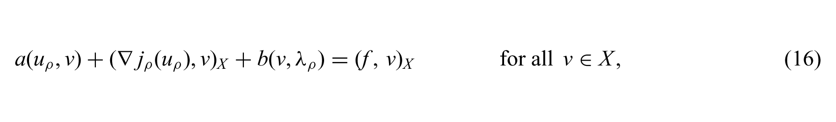
Lemma 2. A pair (u_ρ, λ_ρ) ∈ X×Λ verifies (10) if and only if it verifies

a (u_{ρ}, v) + {(\nabla j_{ρ} (u_{ρ}), v)}_{X} + b (v, λ_{ρ}) = {(f, v)}_{X} f o r a l l v \in X .

(12)

Proof. Since a is a bilinear continuous form we can define A: X → X as follows. For each w ∈ X, Aw is the unique element of X so that

{(A w, v)}_{X} = a (w, v) for all v \in X .

Similarly, since b is a bilinear continuous form, we can define an operator B: Y → X as follows: for each μ ∈ Λ, Bμ is the unique element of X such that

{(B μ, v)}_{X} = b (v, μ) for all v \in X .

Using the operators A and B we can rewrite (10) as follows:

j_{ρ} (v) - j_{ρ} (u_{ρ}) \geq {(f - A u_{ρ} - B λ_{ρ}, v - u_{ρ})}_{X} for all v \in X .

Therefore, f−Au_ρ−Bλ_ρ ∈ ∂j_ρ(u_ρ). Since $j_{ρ} : X \to ℝ$ is convex and Gâteaux differentiable, according to (1) we can write

f - A u_{ρ} - B λ_{ρ} = \nabla j_{ρ} (u_{ρ}) .

Then,

{(f, v)}_{X} - a (u_{ρ}, v) - b (v, λ_{ρ}) = {(\nabla j_{ρ} (u_{ρ}), v)}_{X} for all v \in X

and from this we obtain (12).

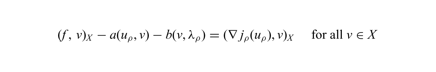
Conversely, by (12) we can write

a (u_{ρ}, v - u_{ρ}) + {(\nabla j_{ρ} (u_{ρ}), v - u_{ρ})}_{X} + b (v - u_{ρ}, λ_{ρ}) = {(f, v - u_{ρ})}_{X} for all v \in X .

(13)

Since, according to Proposition 1, we have

j_{ρ} (v) - j_{ρ} (u_{ρ}) \geq {(\nabla j_{ρ} (u_{ρ}), v - u_{ρ})}_{X} for all v \in X,

(14)

we get (10) combining (14) with (13).

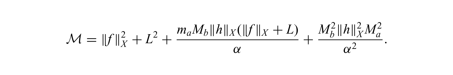
Let us introduce the following notation:

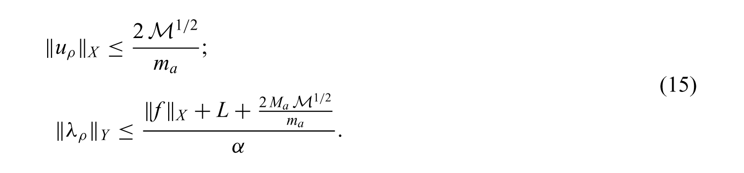
ℳ = ‖ f ‖_{X}^{2} + L^{2} + \frac{m_{a} M_{b} ‖ h ‖_{X} (‖ f ‖_{X} + L)}{α} + \frac{M_{b}^{2} ‖ h ‖_{X}^{2} M_{a}^{2}}{α^{2}} .

Proposition 3. Let ρ > 0. If Assumptions 1 and 3 to 6 hold true, then Problem 3 has a unique solution (u_ρ,λ_ρ). Moreover,

\begin{array}{l} ‖ u_{ρ} ‖_{X} & \leq & \frac{2 ℳ^{1 / 2}}{m_{a}}; \\ ‖ λ_{ρ} ‖_{Y} & \leq & \frac{‖ f ‖_{X} + L + \frac{2 M_{a} ℳ^{1 / 2}}{m_{a}}}{α} . \end{array}

(15)

Proof. By using arguments similar to those used in the proof of Theorem 2, we deduce that Problem 3 has at least one solution.

According to Lemma 2, Problem 3 is equivalent to the following problem: given ρ > 0 and f,h ∈ X, find (u_ρ,λ_ρ) ∈ X × Y such that λ_ρ ∈ Λ ⊂ Y and

a (u_{ρ}, v) + {(\nabla j_{ρ} (u_{ρ}), v)}_{X} + b (v, λ_{ρ}) = {(f, v)}_{X} for all v \in X,

(16)

b (u_{ρ}, μ - λ_{ρ}) \leq b (h, μ - λ_{ρ}) for all μ \in Λ .

(17)

Let us define an operator A_ρ: X → X as follows. For each u ∈ X, A_ρu is the unique element of X such that

{(A_{ρ} u, v)}_{X} = a (u, v) + {(\nabla j_{ρ} (u), v)}_{X} for all v \in X .

Taking into account the properties of a and j_ρ we deduce that the operator A is a strongly monotone and Lipschitz continuous operator. Thus, Problem 3 can be rewritten as follows: given ρ > 0 and f, h ∈ X, find (u_ρ, λ_ρ) ∈ X × Y such that λ_ρ ∈ Λ ⊂ Y and

{(A_{ρ} u_{ρ}, v)}_{X} + b (v, λ_{ρ}) = {(f, v)}_{X} for all v \in X,

(18)

b (u_{ρ}, μ - λ_{ρ}) \leq b (h, μ - λ_{ρ}) for all μ \in Λ .

(19)

As is known (see e.g. [17, 22]) such a generalized saddle point problem has a unique solution which depends Lipschitz continuously on the data (f, h) ∈ X × X. Besides, using arguments similar to those used to prove Proposition 2, we deduce (15).

Corollary 2. Let (u_ρ, λ_ρ)_ρ be a sequence of solutions corresponding to a sequence of regularized problems. There exist (u_ρ′, λ_ρ′)_ρ′ a subsequence of the sequence (u_ρ, λ_ρ)_ρ, and $\tilde{u} \in X,$ $\tilde{λ} \in Λ$ , such that

u_{ρ^{'}} ⇀ \tilde{u} in X as ρ^{'} \to 0

and

λ_{ρ^{'}} ⇀ \tilde{λ} in Y as ρ^{'} \to 0 .

Proof. As L is independent of ρ, by (15) we deduce that (u_ρ)_ρ is a bounded sequence in X and (λ_ρ)_ρ is a bounded sequence in Y. As X and Y are real reflexive Banach spaces, we can subtract weakly convergent subsequences. Since Λ is a closed convex subset of Y, the weak limit $\tilde{λ}$ remains in Λ.

Assumption 7. There exists $ℱ : ℝ_{+} \to ℝ_{+}$ such that:

$ℱ (ρ) \to 0$ as ρ → 0;

For each ρ > 0, $| j_{ρ} (v) - j (v) | \leq ℱ (ρ)$ for all v ∈ X.

Lemma 3. Let u_ρ be the first component of the unique solution pair of Problem 3. Then

u_{ρ} \to u i n X a s ρ \to 0,

where u is the unique first component of a solution pair of Problem 1.

Proof. Let ρ > 0, (u_ρ, λ_ρ), be the unique solution of Problem 3 and (u, λ) be a solution of Problem 1. Setting v = u in (10), μ =λ in (11), v = u_ρ in (2) and μ =λ_ρ in (3), we obtain

a (u_{ρ}, u - u_{ρ}) + j_{ρ} (u) - j_{ρ} (u_{ρ}) + b (u - u_{ρ}, λ_{ρ}) \geq {(f, u - u_{ρ})}_{X}

(20)

b (u_{ρ}, λ - λ_{ρ}) \leq b (h, λ - λ_{ρ})

(21)

a (u, u_{ρ} - u) + j (u_{ρ}) - j (u) + b (u_{ρ} - u, λ) \geq {(f, u_{ρ} - u)}_{X}

(22)

b (u, λ_{ρ} - λ) \leq b (h, λ_{ρ} - λ) .

(23)

Summing (20) and (22) we get

a (u_{ρ} - u, u - u_{ρ}) + j_{ρ} (u) - j_{ρ} (u_{ρ}) + j (u_{ρ}) - j (u) + b (u - u_{ρ}, λ_{ρ}) + b (u_{ρ} - u, λ) \geq 0 .

On the other hand, summing (21) and (23) it follows that

b (u_{ρ} - u, λ - λ_{ρ}) \leq 0 .

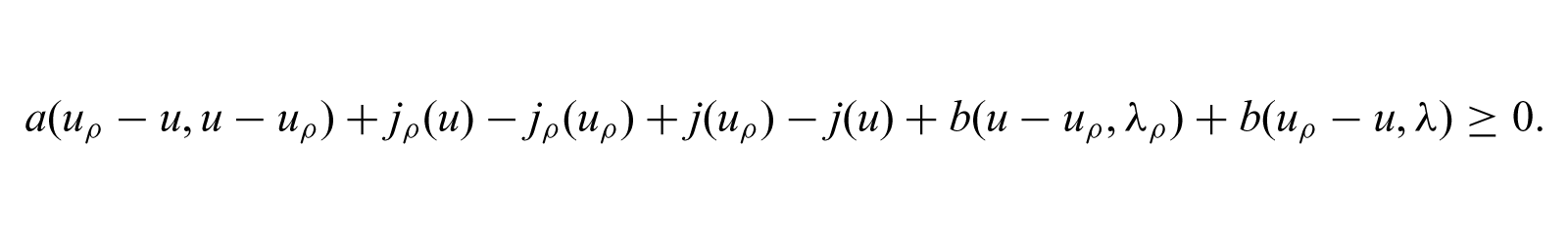
Combining the last two inequalities we have

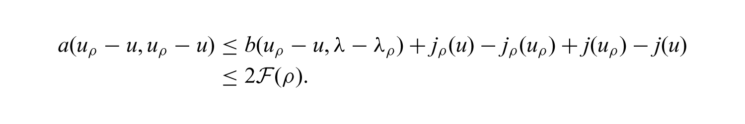
\begin{array}{l} a (u_{ρ} - u, u_{ρ} - u) & \leq & b (u_{ρ} - u, λ - λ_{ρ}) + j_{ρ} (u) - j_{ρ} (u_{ρ}) + j (u_{ρ}) - j (u) \\ \leq & 2 ℱ (ρ) . \end{array}

Therefore,

‖ u_{ρ} - u ‖_{X} \leq \sqrt{\frac{2}{m_{a}} ℱ (ρ)} .

Passing to the limit ρ → 0 we deduce that the sequence (u_ρ)_ρ converges strongly to u in X as ρ → 0.

Corollary 3. The whole sequence (u_ρ)_ρ converges strongly to $\tilde{u} = u$ .

Proof. By Lemma 3, the sequence (u_ρ)_ρ converges weakly to u. As, by Corollary 2, its subsequence ${(u_{ρ^{'}})}_{ρ^{'}}$ is weakly convergent to $\tilde{u}$ , we deduce that $u = \tilde{u}$ . We again use Lemma 3.

Lemma 4. Let (u_ρ, λ_ρ)_ρ be a sequence of solutions of a sequence of regularized problems. Then

j (u_{ρ}) \to j (u) a s ρ \to 0;

(24)

j_{ρ} (u_{ρ}) \to j (u) a s ρ \to 0 .

(25)

Proof. As j is a Lipschitz functional we have

| j (u_{ρ}) - j (u) | \leq L_{j} ‖ u_{ρ} - u ‖_{X},

and from this, since

u_{ρ} \to u in X as ρ \to 0,

we conclude (24). Let us prove (25):

\begin{array}{l} | j_{ρ} (u_{ρ}) - j (u) | & \leq & | j_{ρ} (u_{ρ}) - j (u_{ρ}) | + | j (u_{ρ}) - j (u) | \\ \leq & ℱ (ρ) + | j (u_{ρ}) - j (u) | . \end{array}

Taking into account (24) and Assumption 7, we get (25) passing to limit ρ → 0.

Proposition 4. The pair $(\tilde{u}, \tilde{λ})$ is a solution of Problem 1.

Proof. According to Corollary 2 and Corollary 3 we have $u_{ρ^{'}} \to \tilde{u}$ as ρ′ → 0 in X and $λ_{ρ^{'}} ⇀ \tilde{λ}$ as ρ′ → 0 in Y. Taking into account Assumption 7 and Lemma 4, after passing to the limit ρ′ → 0 in Problem 3 we obtain

a (\tilde{u}, v - \tilde{u}) + j (v) - j (\tilde{u}) + b (v - \tilde{u}, \tilde{λ}) \geq {(f, v - \tilde{u})}_{X} for all v \in X,

(26)

b (\tilde{u}, μ - \tilde{λ}) \leq b (h, μ - \tilde{λ}) for all μ \in Λ .

(27)

Therefore $(\tilde{u}, \tilde{λ})$ is a solution of Problem 1.

Remark 1. We can compute the unique first component of a solution pair of Problem 1 by computing the strong limit of the sequence (u_ρ)_ρ.

3. Statement of the models and hypotheses

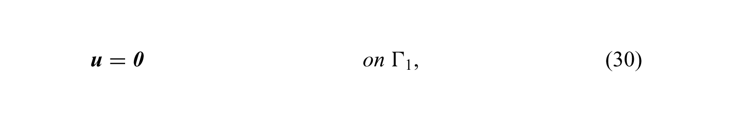
We consider an elastic body that occupies the bounded domain $Ω \subset ℝ^{3}$ , with the boundary partitioned into four measurable parts, Γ₁, Γ₂, Γ₃ and Γ₄, such that meas(Γ₁) > 0. The unit outward normal vector to Γ is denoted by ν and is defined almost everywhere. The body Ω is clamped on Γ₁, body forces of density f ₀ act on Ω and surface traction of density f ₂ acts on Γ₂. On Γ₃ the body is in frictional contact with a foundation and on Γ₄ it can be in contact with a rigid obstacle. We denote the displacement field by u = (u_i), the infinitesimal strain tensor by ε = ε ( u ) = (ε_ij( u )) and the Cauchy stress tensor by σ = (σ_ij). Everywhere below $\bar{Ω}$ denotes Ω ∪ ∂Ω.

According to the physical setting, we can formulate a first mechanical problem as follows.

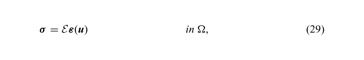
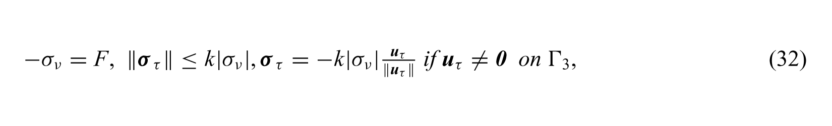
Problem 4. Find $u : \bar{Ω} \to ℝ^{3}$ and $σ : \bar{Ω} \to S^{3}$ such that

Div σ + f_{0} = 0 i n Ω,

(28)

σ = ℰ ε (u) i n Ω,

(29)

u = 0 o n Γ_{1},

(30)

σ ν = f_{2} o n Γ_{2},

(31)

- σ_{ν} = F, ‖ σ_{τ} ‖ \leq k | σ_{ν} |, σ_{τ} = - k | σ_{ν} | \frac{u_{τ}}{‖ u_{τ} ‖} i f u_{τ} \neq 0 o n Γ_{3},

(32)

σ_{τ} = 0, σ_{ν} \leq 0, u_{ν} - g \leq 0, σ_{ν} (u_{ν} - g) = 0 o n Γ_{4},

(33)

where $ℰ$ is the elastic tensor, $F : Γ_{3} \to ℝ_{+}$ denotes the prescribed normal stress, $k : Γ_{3} \to ℝ_{+}$ denotes the coefficient of friction and $g : Γ_{4} \to ℝ_{+}$ denotes the gap.

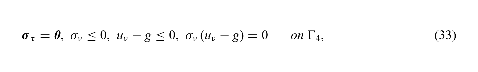
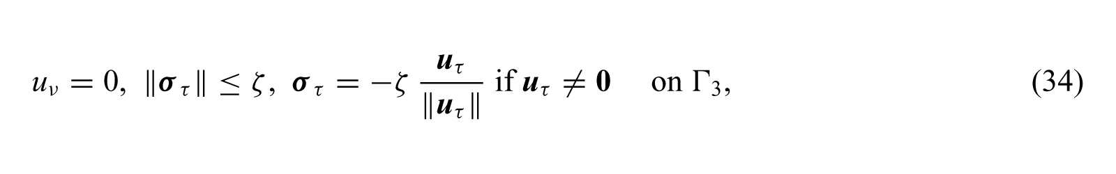
If we assume that on Γ₃ the body is in bilateral frictional contact, we replace (32) with the following condition:

u_{ν} = 0, ‖ σ_{τ} ‖ \leq ζ, σ_{τ} = - ζ \frac{u_{τ}}{‖ u_{τ} ‖} if u_{τ} \neq 0 on Γ_{3},

(34)

where $ζ : Γ_{3} \to ℝ_{+}$ denotes the friction bound. Now, a second model can be formulated as follows.

Problem 5. Find $u : \bar{Ω} \to ℝ^{3}$ and $σ : \bar{Ω} \to S^{3}$ such that (28) to (31), (33) and (34) are satisfied.

We recall that $S^{3}$ denotes the space of second-order symmetric tensors on $ℝ^{3}$ and ‖·‖ denotes the Euclidean norm on $ℝ^{3}$ and $S^{3}$ . Also, we mention here that

ε_{i j} (u) = \frac{1}{2} (u_{i, j} + u_{j, i}), Div σ = (σ_{i j, j}),

the index that follows a comma indicating a partial derivative with respect to the corresponding component of the independent variable. Besides, we recall that the normal and the tangential components of the Cauchy vector σν are given by the formulas σ_ν = ( σν ) · ν and σ _τ = σν − σ_ν ν , while the normal and the tangential components on the boundary of the displacement vector are defined as u_ν = u · ν and u _τ = u − u_ν ν .

Details on the frictional laws and unilateral contact condition can be found for example in [9].

Let us make the following assumptions.

Assumption 8. $ℰ : Ω \times S^{3} \to S^{3}$ is a fourth-order tensor such that:

(i₁) $ℰ_{i j k l} = ℰ_{k l i j} = ℰ_{j i k l} \in L^{\infty} (Ω), 1 \leq i, j, k, l \leq d;$

(i₂) $T h e r e e x i s t s m_{ℰ} > 0 : ℰ τ \cdot τ \geq m_{ℰ} ‖ τ ‖^{2} \forall τ \in S^{3},$ a.e. in Ω.

Assumption 9. The density of the volume forces satisfies f ₀ ∈ L²(Ω)³ and the density of traction satisfies f ₂ ∈ L²(Γ₂)³.

Assumption 10. There exists $g_{e x t} : Ω \to ℝ$ such that g_ext ∈ H¹(Ω), γg_ext = 0 almost everywhere on Γ₁, γg_ext ≥ 0 almost everywhere on Γ\Γ₁ and g = γ g_ext almost everywhere on Γ₄.

As usual, we denoted by γ the Sobolev trace operator γ: H¹(Ω) → L²(Γ).

Assumption 11. The prescribed normal stress satisfies F ∈ L^∞(Γ₃) and F( x ) ≥ 0 a.e. x ∈ Γ₃.

Assumption 12. The coefficient of friction satisfies k ∈ L^∞(Γ₃) and k( x ) ≥ 0 a.e. x ∈ Γ₃.

Assumption 13. The friction bound satisfies ζ ∈ L^∞(Γ₃) and ζ( x ) ≥ 0 a.e. x ∈ Γ₃.

Assumption 14. The unit outward normal to Γ₄ is a constant vector.

4. Weak solvability of Problem 4

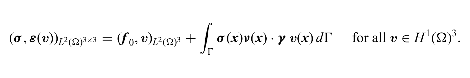
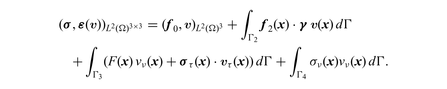
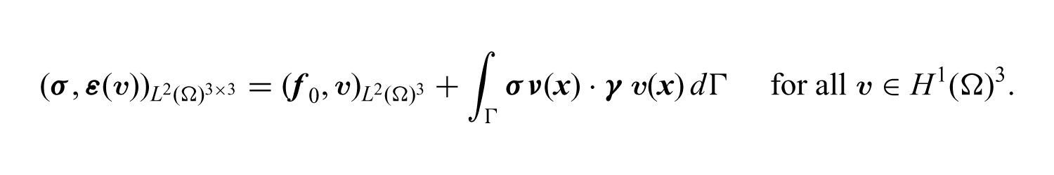
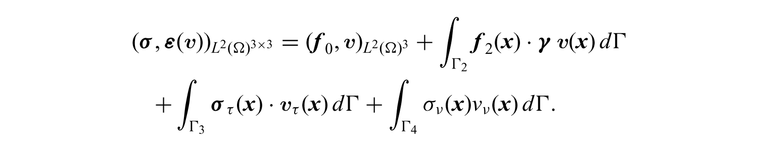
In order to deliver a weak formulation of Problem 4 we assume that u and σ are smooth enough functions which verify (28) to (33). Using a Green’s formula we can write

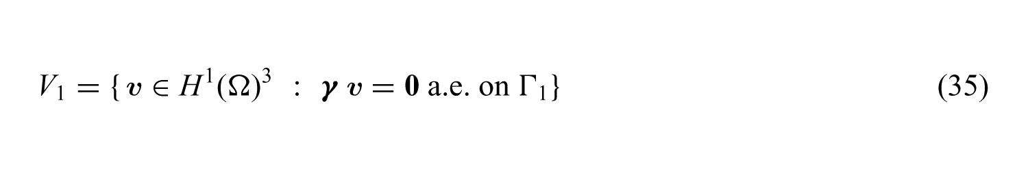
{(σ, ε (v))}_{L^{2} {(Ω)}^{3 \times 3}} = {(f_{0}, v)}_{L^{2} {(Ω)}^{3}} + \int_{Γ} σ (x) ν (x) \cdot γ v (x) d Γ for all v \in H^{1} {(Ω)}^{3} .

Let us introduce the space

V_{1} = {v \in H^{1} {(Ω)}^{3} : γ v = 0 a . e . on Γ_{1}}

(35)

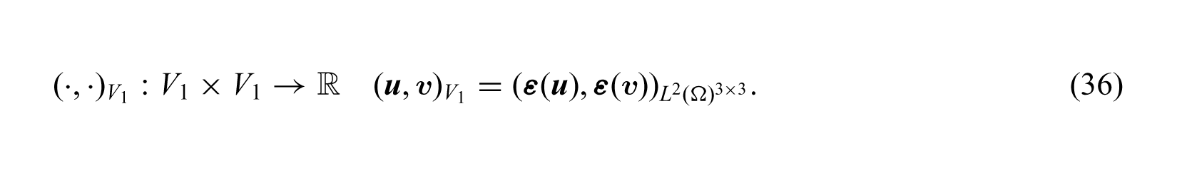
where γ : H¹(Ω)³ → L²(Γ)³ is Sobolev’s trace operator. We recall that γ is a linear and compact operator. The space V₁ is a Hilbert space endowed with the inner product

{(\cdot, \cdot)}_{V_{1}} : V_{1} \times V_{1} \to ℝ {(u, v)}_{V_{1}} = {(ε (u), ε (v))}_{L^{2} {(Ω)}^{3 \times 3}} .

(36)

For all v ∈ V₁ we have

\begin{array}{l} {(σ, ε (v))}_{L^{2} {(Ω)}^{3 \times 3}} = {(f_{0}, v)}_{L^{2} {(Ω)}^{3}} + \int_{Γ_{2}} f_{2} (x) \cdot γ v (x) d Γ \\ + \int_{Γ_{3}} (F (x) v_{ν} (x) + σ_{τ} (x) \cdot v_{τ} (x)) d Γ + \int_{Γ_{4}} σ_{ν} (x) v_{ν} (x) d Γ . \end{array}

Notice that for a field v ∈ H¹(Ω)³, by v_ν we understand γv · ν and by v _τ we understand γ v − v_ν · ν .

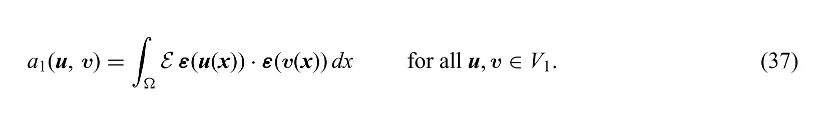
We define a bilinear form $a_{1} : V_{1} \times V_{1} \to ℝ$ so that

a_{1} (u, v) = \int_{Ω} ℰ ε (u (x)) \cdot ε (v (x)) d x for all u, v \in V_{1} .

(37)

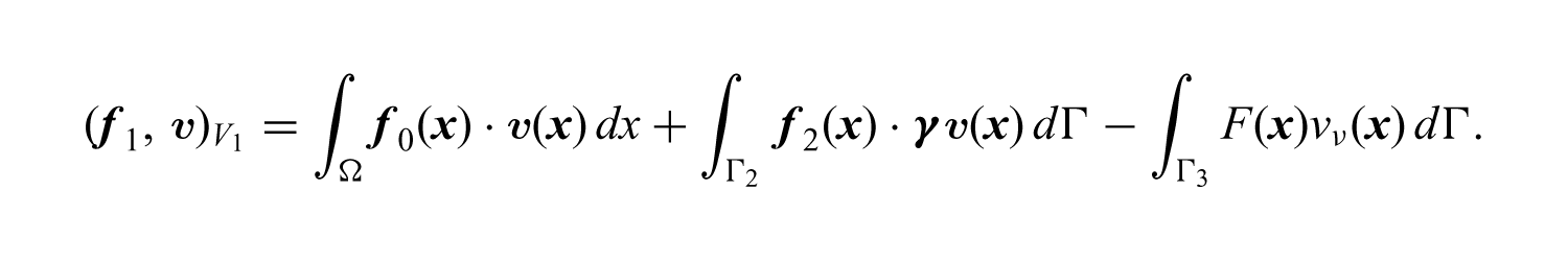
Using Riesz’s representation theorem, we define f ₁ ∈ V₁ such that, for all v ∈ V₁,

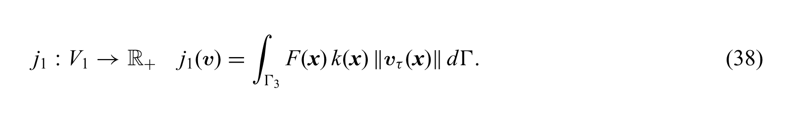
{(f_{1}, v)}_{V_{1}} = \int_{Ω} f_{0} (x) \cdot v (x) d x + \int_{Γ_{2}} f_{2} (x) \cdot γ v (x) d Γ - \int_{Γ_{3}} F (x) v_{ν} (x) d Γ .

Besides, we introduce a functional j₁ as follows:

j_{1} : V_{1} \to ℝ_{+} j_{1} (v) = \int_{Γ_{3}} F (x) k (x) ‖ v_{τ} (x) ‖ d Γ .

(38)

By standard calculus we deduce that, for all v ∈ V₁,

a_{1} (u, v - u) + j_{1} (v) - j_{1} (u) \geq {(f_{1}, v - u)}_{V_{1}} + \int_{Γ_{4}} σ_{τ} (x) \cdot (v_{τ} (x) - u_{τ} (x)) d Γ .

Let D₁ be the dual of the space

M_{1} = {\tilde{v} = v_{ν |_{Γ_{4}}} v \in V_{1}} .

We define λ ∈ D₁ such that

〈 λ, w 〉 = - \int_{Γ_{4}} σ_{ν} (x) w (x) d Γ for all w \in M_{1},

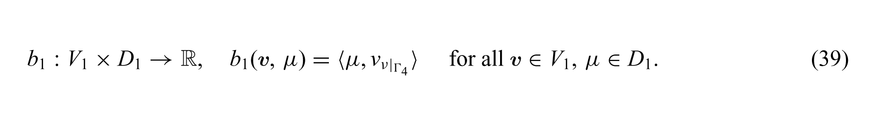
where 〈·,·〉 denotes the duality pairing between D₁ and M₁. Furthermore, we define a bilinear form as follows:

b_{1} : V_{1} \times D_{1} \to ℝ, b_{1} (v, μ) = 〈 μ, v_{ν |_{Γ_{4}}} 〉 for all v \in V_{1}, μ \in D_{1} .

(39)

Let us introduce the following subset of D₁:

Λ_{1} = {μ \in D_{1} : 〈 μ, v_{ν |_{Γ_{4}}} 〉 \leq 0 for all v \in K_{1}},

(40)

where

K_{1} = {v \in V_{1} : v_{ν} \leq 0 almost everywhere on Γ_{4}} .

It is easy to observe that λ ∈ Λ₁. Moreover, by (33) it follows that

b_{1} (u, λ) = b_{1} (g_{e x t} ν_{4}, λ)

and, by (40),

b_{1} (u, μ) \leq b_{1} (g_{e x t} ν_{4}, μ) for all μ \in Λ_{1};

here and below ν ₄ denotes $ν |_{Γ_{4}}$ which according to Assumption 14 is a constant vector. Notice that Assumption 14 allows us to write b₁(g_ext ν ₄, λ) = 〈λ, g〉 and b₁(g_ext ν ₄, μ) = 〈μ, g〉.

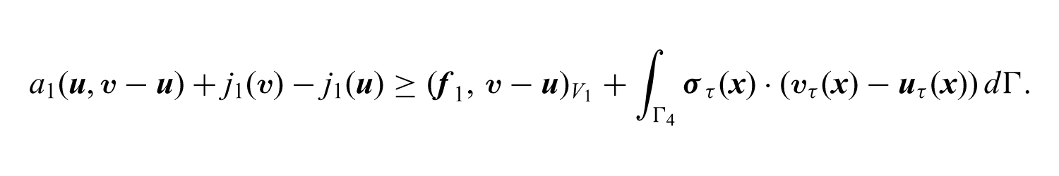
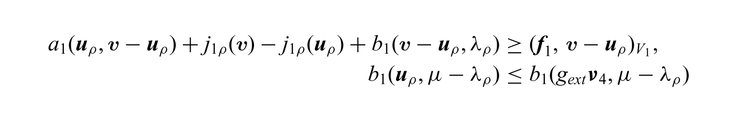
We are led to the following weak formulation of Problem 4.

Problem 6. Find u ∈ V₁ and λ ∈ Λ₁ such that, for all v ∈ V₁, μ ∈ Λ₁,

\begin{array}{l} a_{1} (u, v - u) + j_{1} (v) - j_{1} (u) + b_{1} (v - u, λ) & \geq & {(f_{1}, v - u)}_{V_{1}}, \\ b_{1} (u, μ - λ) & \leq & b_{1} (g_{e x t} ν_{4}, μ - λ) . \end{array}

A solution of Problem 6 is called a weak solution to Problem 4. The well-posedness of Problem 6 is given by the following theorem.

Theorem 3. If Assumptions 8 to 12 and 14 hold, then Problem 6 has a bounded solution ( u , λ) ∈ V₁ × Λ₁, unique in its first argument.

Proof. Let us use X = V₁, Y = D₁, f = f ₁, a = a₁, b = b₁, j = j₁ and Λ = Λ₁. Due to Assumption 8, the form a₁ fulfills Assumption 1. Besides, the functional j₁ defined by (38) fulfills Assumption 2. On the other hand, by standard arguments (see e.g. [17]), it can be proved that the form b₁ fulfills Assumption 3. Also, the set Λ₁ defined by (40) fulfills Assumption 4.

Apply Theorem 2 and Proposition 2.

Let ρ > 0. We consider the following regularized problem.

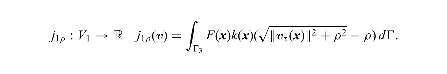
Problem 7. Find u _ρ ∈ V₁ and λ_ρ ∈ Λ₁ such that, for all v ∈ V₁, μ ∈ Λ₁,

\begin{array}{l} a_{1} (u_{ρ}, v - u_{ρ}) + j_{1 ρ} (v) - j_{1 ρ} (u_{ρ}) + b_{1} (v - u_{ρ}, λ_{ρ}) & \geq & {(f_{1}, v - u_{ρ})}_{V_{1}}, \\ b_{1} (u_{ρ}, μ - λ_{ρ}) & \leq & b_{1} (g_{e x t} ν_{4}, μ - λ_{ρ}) \end{array}

where

j_{1 ρ} : V_{1} \to ℝ j_{1 ρ} (v) = \int_{Γ_{3}} F (x) k (x) (\sqrt{‖ v_{τ} (x) ‖^{2} + ρ^{2}} - ρ) d Γ .

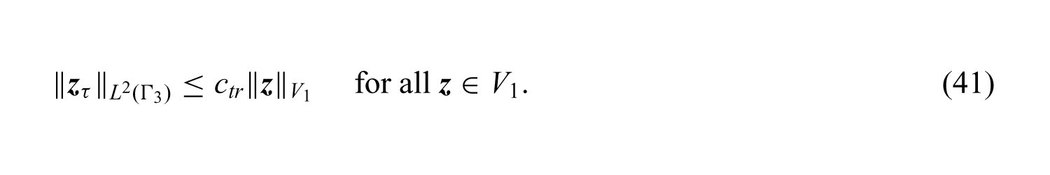
Following [9], useful properties of the functional j_1ρ can be established. First of all, we note that the functional j_1ρ is Gâteaux differentiable. Denoting by ∇j_1ρ its Gâteaux differential we have

$\nabla j_{1 ρ} : V_{1} \to V_{1} {(\nabla j_{1 ρ} (w), v)}_{V_{1}} = \int_{Γ_{3}} F (x) k (x) \frac{w_{τ} (x) \cdot v_{τ} (x)}{\sqrt{‖ w_{τ} (x) ‖^{2} + ρ^{2}}} d Γ;$

$\begin{matrix} ‖ \nabla j_{1 ρ} (v) - \nabla j_{1 ρ} (w) ‖_{V_{1}} = \sup_{z \in V_{1}, z \neq 0_{V_{1}}} \frac{{(\nabla j_{1 ρ} (v) - \nabla j_{1 ρ} (w), z)}_{V_{1}}}{‖ z ‖_{V_{1}}} \\ \leq \frac{2 c_{t r}^{2} ‖ k F ‖_{L^{\infty} (Γ_{3})}}{ρ} ‖ v - w ‖_{V_{1}} for all w, v \in V_{1}, \end{matrix}$

where c_tr is a positive constant which fulfills the following inequality:

‖ z_{τ} ‖_{L^{2} (Γ_{3})} \leq c_{t r} ‖ z ‖_{V_{1}} for all z \in V_{1} .

(41)

In addition, for all v ∈ V₁,

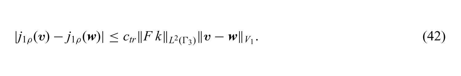
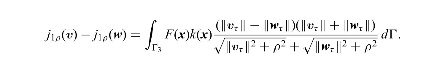
| j_{1 ρ} (v) - j_{1} (v) | \leq ℱ (ρ) where ℱ (ρ) = ρ \int_{Γ_{3}} F (x) k (x) d Γ .

Let us prove that, for all v , w ∈ V₁, we have

| j_{1 ρ} (v) - j_{1 ρ} (w) | \leq c_{t r} ‖ F k ‖_{L^{2} (Γ_{3})} ‖ v - w ‖_{V_{1}} .

(42)

Indeed, for all v , w ∈ V₁,

j_{1 ρ} (v) - j_{1 ρ} (w) = \int_{Γ_{3}} F (x) k (x) \frac{(‖ v_{τ} ‖ - ‖ w_{τ} ‖) (‖ v_{τ} ‖ + ‖ w_{τ} ‖)}{\sqrt{‖ v_{τ} ‖^{2} + ρ^{2}} + \sqrt{‖ w_{τ} ‖^{2} + ρ^{2}}} d Γ .

Since

| ‖ v_{τ} ‖ - ‖ w_{τ} ‖ | \leq ‖ v_{τ} - w_{τ} ‖

and

\frac{‖ v_{τ} ‖ + ‖ w_{τ} ‖}{\sqrt{‖ v_{τ} ‖^{2} + ρ^{2}} + \sqrt{‖ w_{τ} ‖^{2} + ρ^{2}}} \leq 1

we get

| j_{1 ρ} (v) - j_{1 ρ} (w) | \leq \int_{Γ_{3}} F (x) k (x) ‖ v_{τ} (x) - w_{τ} (x) ‖ d Γ,

and from this we deduce (42). Then, there exists $L_{j_{1 ρ}} > 0$ independent of ρ such that Assumption 6 is fulfilled; we can take $L_{j_{1 ρ}} = c_{t r} ‖ k F ‖_{L^{2} (Γ_{3})}$ .

Hence, the functional j_1ρ verifies Assumptions 5, 6 and 7.

According to Theorem 4, the unique weak limit $(\tilde{u}, \tilde{λ})$ of the sequence ( u _ρ, λ_ρ)_ρ ⊂ V₁ × Λ₁, is a solution of Problem 6.

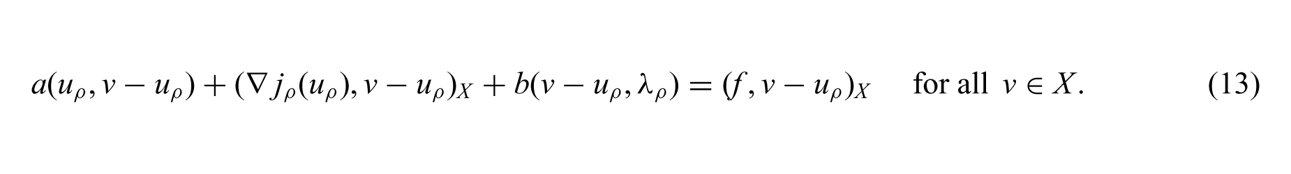
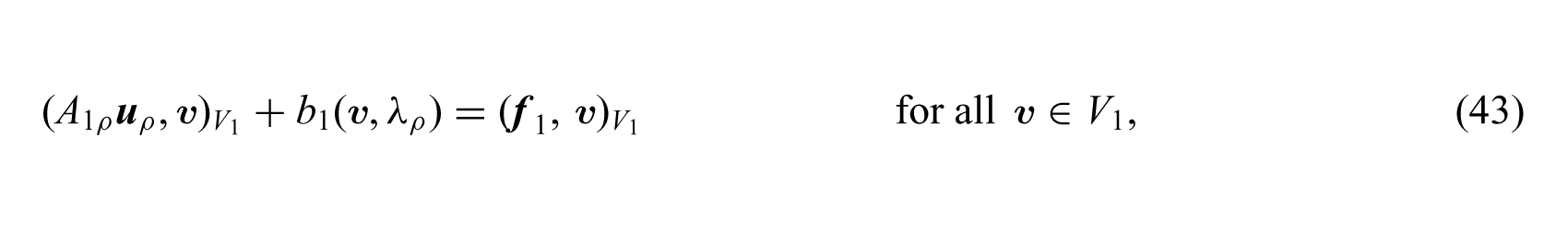
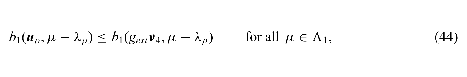
It is worth emphasizing that ( u _ρ, λ_ρ) ∈ V₁ × Λ₁ is a solution of Problem 7 if and only if it verifies

{(A_{1 ρ} u_{ρ}, v)}_{V_{1}} + b_{1} (v, λ_{ρ}) = {(f_{1}, v)}_{V_{1}} for all v \in V_{1},

(43)

b_{1} (u_{ρ}, μ - λ_{ρ}) \leq b_{1} (g_{e x t} ν_{4}, μ - λ_{ρ}) for all μ \in Λ_{1},

(44)

where $A_{1 ρ} : V_{1} \to V_{1}, {(A_{1 ρ} v, w)}_{V_{1}} = a_{1} (v, w) + {(\nabla j_{1 ρ} (v), w)}_{V_{1}}$ .

Remark 2. According to Section 2.2, the first component of a solution of Problem 6 (which is unique in the first argument) is the strong limit of the sequence ( u _ρ)_ρ, u _ρ being the first component of the solution to the problem (43)–(44).

4.1. Weak solvability of Problem 5

In order to deliver a weak formulation of Problem 5 we assume that u and σ are smooth enough functions which verify (28) to (31), (33) and (34). Again using Green’s formula we have

{(σ, ε (v))}_{L^{2} {(Ω)}^{3 \times 3}} = {(f_{0}, v)}_{L^{2} {(Ω)}^{3}} + \int_{Γ} σν (x) \cdot γ v (x) d Γ for all v \in H^{1} {(Ω)}^{3} .

Let us introduce the space

V_{2} = {v \in V_{1} | v_{ν} = 0 almost everywhere on Γ_{3}}

which is a closed subspace of the space V₁ defined in (35).

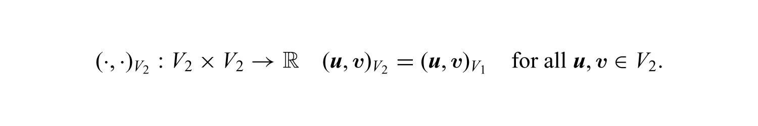
Obviously, $(V_{2}, {(\cdot, \cdot)}_{V_{2}}, ‖ \cdot ‖_{V_{2}})$ is a Hilbert space, where

{(\cdot, \cdot)}_{V_{2}} : V_{2} \times V_{2} \to ℝ {(u, v)}_{V_{2}} = {(u, v)}_{V_{1}} for all u, v \in V_{2} .

For all v ∈ V₂ we have

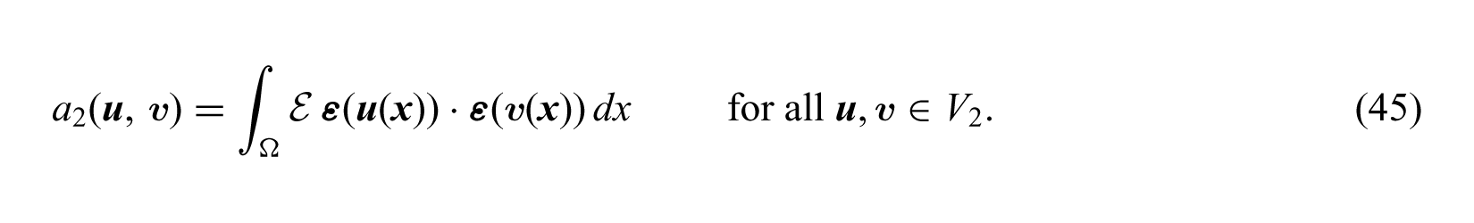
\begin{array}{l} {(σ, ε (v))}_{L^{2} {(Ω)}^{3 \times 3}} = {(f_{0}, v)}_{L^{2} {(Ω)}^{3}} + \int_{Γ_{2}} f_{2} (x) \cdot γ v (x) d Γ \\ + \int_{Γ_{3}} (F (x) v_{ν} (x) + σ_{τ} (x) \cdot v_{τ} (x)) d Γ + \int_{Γ_{4}} σ_{ν} (x) v_{ν} (x) d Γ . \end{array}

We define a bilinear form $a_{2} : V_{2} \times V_{2} \to ℝ$ such that

a_{2} (u, v) = \int_{Ω} ℰ ε (u (x)) \cdot ε (v (x)) d x for all u, v \in V_{2} .

(45)

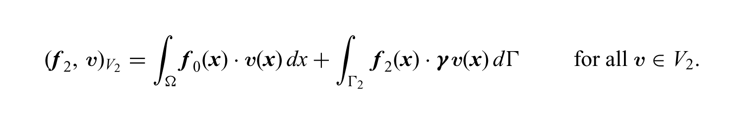
Using Riesz’s representation theorem, we define f ₂ ∈ V₂ such that

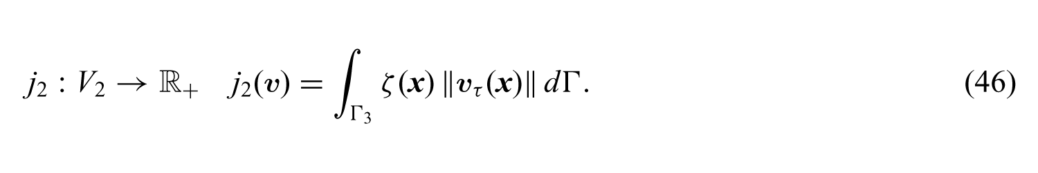
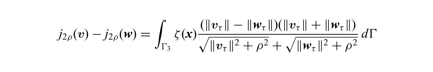
{(f_{2}, v)}_{V_{2}} = \int_{Ω} f_{0} (x) \cdot v (x) d x + \int_{Γ_{2}} f_{2} (x) \cdot γ v (x) d Γ for all v \in V_{2} .

Besides, we introduce a functional j₂ as follows:

j_{2} : V_{2} \to ℝ_{+} j_{2} (v) = \int_{Γ_{3}} ζ (x) ‖ v_{τ} (x) ‖ d Γ .

(46)

By standard calculus we deduce that, for all v ∈ V₂,

a_{2} (u, v - u) + j_{2} (v) - j_{2} (u) \geq {(f_{2}, v - u)}_{V_{2}} + \int_{Γ_{4}} σ_{ν} (x) (v_{ν} (x) - u_{ν} (x)) d Γ .

Let D₂ be the dual of the space

M_{2} = {\tilde{v} = v_{ν |_{Γ_{4}}} v \in V_{2}} .

We define λ ∈ D₂ such that

〈 λ, w 〉 = - \int_{Γ_{4}} σ_{ν} (x) w (x) d Γ for all w \in M_{2},

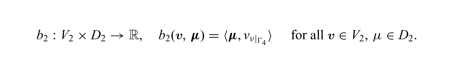
where 〈·,·〉 denotes the duality pairing between D₂ and M₂. Furthermore, we define a bilinear form as follows:

b_{2} : V_{2} \times D_{2} \to ℝ, b_{2} (v, μ) = 〈 μ, v_{ν |_{Γ_{4}}} 〉 for all v \in V_{2}, μ \in D_{2} .

Let us introduce the following subset of D₂,

Λ_{2} = {μ \in D_{2} : 〈 μ, w 〉 \leq 0 for all w \in K},

where

K = {w \in M_{2} : w \leq 0 almost everywhere on Γ_{4}} .

Notice that λ ∈ Λ₂. Moreover,

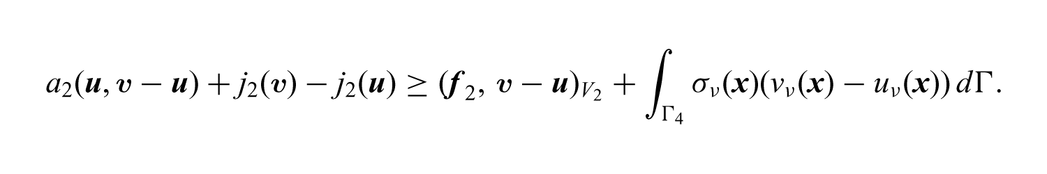
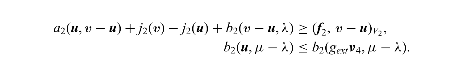
\begin{array}{l} b_{2} (u, λ) & = & b_{2} (g_{e x t} ν_{4}, λ) \\ b_{2} (u, μ) & \leq & b_{2} (g_{e x t} ν_{4}, μ) for all μ \in Λ_{2} . \end{array}

Consequently, we are led to the following weak formulation of Problem 5.

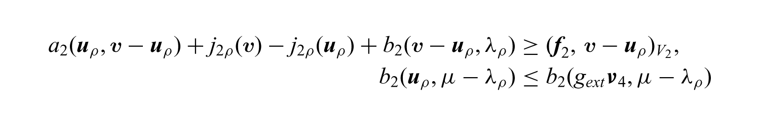
Problem 8. Find u ∈ V₂ and λ ∈ Λ₂ such that, for all v ∈ V₂, μ ∈ Λ₂,

\begin{array}{l} a_{2} (u, v - u) + j_{2} (v) - j_{2} (u) + b_{2} (v - u, λ) & \geq & {(f_{2}, v - u)}_{V_{2}}, \\ b_{2} (u, μ - λ) & \leq & b_{2} (g_{e x t} ν_{4}, μ - λ) . \end{array}

A solution of Problem 8 is called a weak solution to Problem 5.

The well-posedness of Problem 8 is given by the following theorem.

Theorem 4. Assumptions 8 to 10 and Assumptions 13 and 14 hold. Then, Problem 8 has a bounded solution ( u , λ) ∈ V₂ × Λ₂, unique in its first argument.

Proof. Let us set X = V₂, Y = D₂, f = f ₂, a = a₂, b = b₂, j = j₂ and Λ =Λ₂. Due to Assumption 8, the form a₂ fulfills Assumption 1. Besides, the functional j₂ defined by (46) fulfills Assumption 2. On the other hand, the form b₂ fulfills Assumption 3. Also, the set Λ₂ fulfills Assumption 4.

Apply Theorem 2 and Proposition 2.

Let ρ > 0. We consider the following regularized problem.

Problem 9. Let ρ > 0. Find u _ρ ∈ V₂ and λ_ρ ∈ Λ₂ such that for all v ∈ V₂, μ ∈ Λ₂,

\begin{array}{l} a_{2} (u_{ρ}, v - u_{ρ}) + j_{2 ρ} (v) - j_{2 ρ} (u_{ρ}) + b_{2} (v - u_{ρ}, λ_{ρ}) & \geq & {(f_{2}, v - u_{ρ})}_{V_{2}}, \\ b_{2} (u_{ρ}, μ - λ_{ρ}) & \leq & b_{2} (g_{e x t} ν_{4}, μ - λ_{ρ}) \end{array}

where $j_{2 ρ} : V_{2} \to ℝ$ , $j_{2 ρ} (v) = \int_{Γ_{3}} ζ (x) (\sqrt{‖ v_{τ} (x) ‖^{2} + ρ^{2}} - ρ) d Γ$ .

The functional j_2ρ is Gâteaux differentiable. Denoting its Gâteaux differential by ∇j_2ρ we have:

$\nabla j_{2 ρ} : V_{2} \to V_{2} {(\nabla j_{2 ρ} (w), v)}_{V_{2}} = \int_{Γ_{3}} ζ (x) \frac{w_{τ} (x) \cdot v_{τ} (x)}{\sqrt{‖ w_{τ} (x) ‖^{2} + ρ^{2}}} d Γ;$

$\begin{matrix} ‖ \nabla j_{2 ρ} (v) - \nabla j_{2 ρ} (w) ‖_{V_{2}} = \sup_{z \in V_{2}, z \neq O_{V_{2}}} \frac{{(\nabla j_{2 ρ} (v) - \nabla j_{2 ρ} (w), z)}_{V_{2}}}{‖ z ‖_{V_{2}}} \\ \leq \frac{2 c_{t r}^{2} ‖ ζ ‖_{L^{\infty} (Γ_{3})}}{ρ} ‖ v - w ‖_{V_{2}} for all w, v \in V_{2} . \end{matrix}$

Furthermore,

| j_{2 ρ} (v) - j_{2} (v) | \leq ℱ (ρ) where ℱ (ρ) = ρ \int_{Γ_{3}} ζ (x) d Γ .

Besides, for all v , w ∈ V₂, we have

j_{2 ρ} (v) - j_{2 ρ} (w) = \int_{Γ_{3}} ζ (x) \frac{(‖ v_{τ} ‖ - ‖ w_{τ} ‖) (‖ v_{τ} ‖ + ‖ w_{τ} ‖)}{\sqrt{‖ v_{τ} ‖^{2} + ρ^{2}} + \sqrt{‖ w_{τ} ‖^{2} + ρ^{2}}} d Γ

and from this, by arguments similar to those used in the previous section, we deduce that there exists $L_{j_{2 ρ}} > 0$ independent of ρ such that

| j_{2 ρ} (v) - j_{2 ρ} (w) | \leq L_{j_{2 ρ}} ‖ v - w ‖_{V_{2}} .

Thus, Assumption 6 is fulfilled; we can take $L_{j_{2 ρ}} = c_{t r} ‖ ζ ‖_{L^{2} (Γ_{3})}$ . Hence, it follows that the functional j_2ρ verifies Assumptions 5, 6 and 7.

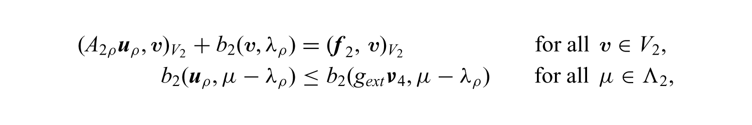
It is worth emphasizing that ( u _ρ, λ_ρ) ∈ V₂ × Λ₂ is a solution of Problem 7 if and only if it verifies

\begin{array}{l} {(A_{2 ρ} u_{ρ}, v)}_{V_{2}} + b_{2} (v, λ_{ρ}) & = & {(f_{2}, v)}_{V_{2}} & for all v \in V_{2}, \\ b_{2} (u_{ρ}, μ - λ_{ρ}) & \leq & b_{2} (g_{e x t} ν_{4}, μ - λ_{ρ}) & for all μ \in Λ_{2}, \end{array}

where $A_{2 ρ} : V_{2} \to V_{2}, {(A_{2 ρ} v, w)}_{V_{2}} = a_{2} (v, w) + {(\nabla j_{2 ρ} (v), w)}_{V_{2}}$ .

Remark 3. The unique first component of a solution pair of Problem 8 is the strong limit of the sequence ( u _ρ)_ρ.

Footnotes

Funding

This work was supported by a grant from the Romanian National Authority for Scientific Research, CNCS-UEFISCDI (project number PN-II-RU-TE-2011-3-0223).

References

Duvaut

Lions

J-L

. Inequalities in mechanics and physics. Berlin: Springer-Verlag, 1976.

Eck

Jarušek

Krbeč

. Unilateral contact problems: Variational methods and existence theorems (Pure and Applied Mathematics, vol. 270). New York, NY: Chapman/CRC Press, 2005.

Kikuchi

Oden

. Contact problems in elasticity: A study of variational inequalities and finite element methods. Philadelphia, PA: SIAM, 1988.

Han

Sofonea

. Quasistatic contact problems in viscoelasticity and viscoplasticity (Studies in Advanced Mathematics, vol. 30). Providence, RI: American Mathematical Society/International Press, 2002.

Migorski

Ochal

Sofonea

. Nonlinear inclusions and hemivariational inequalities (Advances in Mechanics and Mathematics, vol. 26). New Yor, NY: Springer, 2013.

Shillor

Sofonea

Telega

. Models and variational analysis of quasistatic contact (Lecture Notes in Physics, vol. 655). Berlin/Heidelberg: Springer, 2004.

Sofonea

Han

Shillor

. Analysis and approximation of contact problems with adhesion or damage (Pure and Applied Mathematics, vol. 276). New York, NY: Chapman-Hall/CRC Press, 2006.

Sofonea

Matei

. Variational inequalities with applications: A study of antiplane frictional contact problems (Advances in Mechanics and Mathematics, vol. 18). New York, NY: Springer, 2009.

Sofonea

Matei

. Mathematical models in contact mechanics (London Mathematical Society Lecture Note Series, vol. 398). Cambridge: Cambridge University Press, 2012.

10.

Wriggers

. Computational contact mechanics. 2nd edn. Heidelberg: Springer, 2006.

11.

Laursen

. Computational contact and impact mechanics. New York, NY: Springer, 2002.

12.

Adams

. Sobolev spaces. New York, NY: Academic Press, 1975.

13.

Brézis

. Analyse fonctionnelle – Théorie et applications. Paris: Masson, 1987.

14.

Grisvard

. Elliptic problems in nonsmooth domains (Monographs and Studies in Mathematics, vol. 24). Boston, MA: Pitman, 1985.

15.

Lions

J-L

Magenes

. Problèmes aux limites non homogènes. Paris: Dunod, 1968.

16.

Matei

. A variational approach for an electro-elastic unilateral contact problem. Math Modell Anal 2009; 14(3): 323–334.

17.

Matei

Ciurcea

. Contact problems for nonlinearly elastic materials: Weak solvability involving dual Lagrange multipliers. ANZIAM J 2010; 52: 160–178.

18.

Matei

Ciurcea

. Weak solvability for a class of contact problems. Ann Acad Roman Sci Ser Math Appl 2010; 2(1): 25–44.

19.

Matei

Ciurcea

. Weak solutions for contact problems involving viscoelastic materials with long memory. Math Mech Solids 2011; 16(4): 393–405.

20.

Matei

. On the solvability of mixed variational problems with solution-dependent sets of Lagrange multipliers. Proc R Soc Edinb A Math 2013; 143: 1047–1059.

21.

Matei

. An evolutionary mixed variational problem arising from frictional contact mechanics. Math Mech Solids 2014; 19: 225–241.

22.

Matei

. Weak solvability via Lagrange multipliers for two frictional contact models. In: Proceedings of the 11th French–Romanian conference on applied mathematics, 2012.

23.

Amdouni

Hild

Lleras

. A stabilized Lagrange multiplier method for the enriched finite-element approximation of contact problems of cracked elastic bodies. ESAIM: Math Modell Numer Anal 2012; 46: 813–839.

24.

Barboteu

Matei

Sofonea

. On the behavior of the solution of a viscoplastic contact problem. Q Appl Math. 2014; 72 (4): 625–647.

25.

Hild

Renard

. A stabilized Lagrange multiplier method for the finite element approximation of contact problems in elastostatics. Numer Math 2010; 115: 101–129.

26.

Hüeber

Matei

Wohlmuth

. A mixed variational formulation and an optimal a priori error estimate for a frictional contact problem in elasto-piezoelectricity. Bull Math Soc Sci Math Rouman 2005; 48: 209–232.

27.

Hüeber

Matei

Wohlmuth

. Efficient algorithms for problems with friction. SIAM J Sci Comput 2007; 29: 70–92.

28.

Hüeber

Wohlmuth

. An optimal a priori error estimate for non-linear multibody contact problems. SIAM J Numer Anal 2005; 43(1): 157–173.

29.

Hüeber

Wohlmuth

. A primal-dual active set strategy for non-linear multibody contact problems. Comput Meth Appl Mech Eng 2005; 194: 3147–3166.

30.

Hüeber

Matei

Wohlmuth

. A contact problem for electro-elastic materials. Z Angew Math Mech 2013; 93: 789–800.

31.

Ciurcea

Matei

. Solvability of a mixed variational problem. Ann Univ Craiova 2009; 36(1): 105–111.

32.

Ekeland

Temam

. Convex analysis and variational problems. Amsterdam: North-Holland, 1976.

33.

Niculescu

Persson

L-E

. Convex functions and their applications: A contemporary approach (CMS Books in Mathematics, vol. 23). New York, NY: Springer-Verlag, 2006.

34.

Braess

. Finite elements. Cambridge: Cambridge University Press, 1997.

35.

Brezzi

Fortin

. Mixed and hybrid finite element methods. New York, NY: Springer-Verlag, 1991.

36.

Haslinger

Hlavácek

Necas

. Numerical methods for unilateral problems in solid mechanics. In Ciarlet

Lions

(eds.) Handbook of numerical analysis, volume 4. Amsterdam: North-Holland, 1996, 313–485.

37.

Quarteroni

Valli

. Numerical approximation of partial differential equations. Berlin/Heidelberg: Springer-Verlag, 2008.

38.

Laborde

Renard

. Fixed point strategies for elastostatic frictional contact problems. Math Meth Appl Sci 2008; 31: 415–441.